Learning to Rasterize Differentiable

Abstract

Differentiable rasterization changes the common formulation of primitive rasterization —which has zero gradients almost everywhere, due to discontinuous edges and occlusion— to an alternative one, which is not subject to this limitation and has similar optima. These alternative versions in general are ”soft” versions of the original one. Unfortunately, it is not clear, what exact way of softening will provide the best performance in terms of converging the most reliability to a desired goal. Previous work has analyzed and compared several combinations of softening. In this work, we take it a step further and, instead of making a combinatorical choice of softening operations, parametrize the continuous space of all softening operations. We study meta-learning a parametric S-shape curve as well as an MLP over a set of inverse rendering tasks, so that it generalizes to new and unseen differentiable rendering tasks with optimal softness.

1 Introduction

While forward rendering generates a 2D image based on 3D scene parameters, inverse rendering optimizes these parameters to reproduce the given 2D image given as a reference. When wishing to employ modern gradient-based optimizers, the rendering has to be made differentiable to enable applications such as model reconstruction [5], pose estimation [9, 4], lighting and materials estimation [2, 10]. Differentiation is difficult due to the presence of discontinuities.

The renderer can be generally differentiated in two main ways. Either by approximating the gradients using the exact forward rendering process which may need a manual design for gradients, or directly approximating the forward rendering process which enables Automatic Differentiation (AD). To approximate the gradients, Loper and Black [9] leverages the difference of neighboring pixels and similar Kato et al. [5] with a hand-crafted function. Li et al. [7] proposed integrating the gradients using Monte Carlo ray tracing. In contrast, other lines of works are naturally differentiable using probabilistic perturbation. Rhodin et al. [15] introduced using sigmoid distributions to blur the rasterization and approximate the rasterized value as a density parameter to control the transparency of blobby objects. Later studies use different functions such as the square root of a logistic distribution [8] and logistic distribution [12] in a similar way.

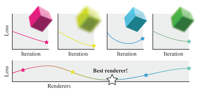
Figure 1: Out of continuously many differentiable rasterizers, we find the one that is best to solve a family of inverse rendering tasks.

All these soft variants of rasterization have enabled effective inverse rendering, overcoming the challenge of discontinuities. However, finding the right softness function remains challenging. We argue that there is no single right function, that the choice of softness depends on the problem and that adaptation to the problem should be automated and systematic.

In this work, we propose a principled way to tackle this problem on another level of abstraction. We do not look at individual inverse rendering problems, but at the set of all problems. Given a training set of inverse rendering problems, we identify the best way, in terms of convergence speed and/or quality, to change the renderer. In this way, the renderer gets differentiable, specific to the task at hand.

Concretely, we introduce meta-learning to learn the optimal edge and occlusion softness in the differentiable rasterizer. We show that the resulting method outperforms state-of-the-art methods that all chose a manual softness scale for a given parametric distribution. We meta-tune both a parametric S-shape curve and a more general Multi-layer Perceptron (MLP).

2 Background

Differentiable rendering allows computing gradients of 3D scene parameters with respect to the image pixels.

2.1 Problem setting

mymaths $\mathcal{R}_{\mathrm{h}}$ mymaths $\mathcal{R}_{\mathrm{s}}$ mymaths $\theta$ mymaths $\theta^{\star}$ mymaths $\mathtt{opt}$ mymaths $I$ mymaths $\phi$ mymaths $\phi^{\star}$ mymaths $m$ mymaths $n$ mymaths $\lambda$ mymaths $\lambda_{\theta}$ mymaths $\lambda_{\phi}$

Let $\mathcal{R}_{\mathrm{h}}$ be a common renderer that takes scene parameters $\theta$ and maps them to an image. Differentiating this function is not possible due to the discontinuity of the parameters and gradients which are zero almost everywhere. Hence the subscript $h$, for ”hard”. Formally, let $\theta^{\star}$ be the optimal scene parameters for an image $I$ . Then, unfortunately,

$$\mathtt{opt}(||\mathcal{R}_{\mathrm{h}}(\theta)-I||_{2},\theta)\neq\theta^{\star},$$

where $\mathtt{opt}()$ is an optimizer, such as gradient descent that minimizes the first argument (here, the image difference of rendering and reference image) by changing the second argument (here, the scene parameters). A differentiable renderer $\mathcal{R}_{\mathrm{s}}$ , would exactly provide this, as in

$$\mathtt{opt}(||\mathcal{R}_{\mathrm{s}}(\theta)-I||_{2},\theta)=\theta^{\star}\,.$$

In general $\mathcal{R}_{\mathrm{s}}$ and $\mathcal{R}_{\mathrm{h}}$ are not identical and so the target function we optimize has changed. Alas, the soft version has non-zero gradients everywhere, and the hope is that these gradients will lead to the same, the true, optimum. On an abstract level, this is the first key observation of this work: it does not matter if $\mathcal{R}_{\mathrm{s}}$ and $\mathcal{R}_{\mathrm{h}}$ are the same function, as long as they have the same minima when using the gradients of the soft one in a gradient-based optimization. If we are free to change the renderer, what is a systematic way to go about that? We are trying to replace a function with another one, that can be differentiated and when doing so, results in similar minima.

The two dominant forms of rendering are path tracing and rasterization. Differentiable Monte Carlo path-tracing, which can handle all forms of illumination with enough computation effort, is explored in other work [7, 18]. We here focus on differentiable rasterization, as a specific kind of renderer, that is limited to direct rendering but can be computed efficiently.

2.2 Differentiable rasterization

In this section, we will first discuss rasterization before explaining how to differentiate it.

Hard rasterization:  Rasterization takes a set of 2D triangles with depth and attributes (such as colors) defined at vertices, and decides the attributes of each pixel in a 2D image. A common approach is using an edge function [14] and testing if a pixel is on the right hand side of the three equations that describe the primitive edges. If so, the attributes of the pixel are hard-assigned according to the corresponding to whether they are inside a face of triangle or not. Therefore, pixels are assigned to binary values using a Heaviside step function at the edges which is not differentiable because the gradient is zero everywhere except the jump where the gradient is not even defined.

Furthermore, if multiple primitives fall onto the same pixel, the selected attribute is the one of the closest primitives and the other ones are discarded by $z$-buffering. Unfortunately, this process is also not differentiable.

mymaths $h$ mymaths $s$ mymaths $d$ mymaths 0pt This means that differentiating rasterization means handling both occlusion and edge tests which boils down to differentiating through a function $h(d)\in\mathbb{R}^{+}\rightarrow\mathbb{R}^{+}$ where $d$ is a distance, that could be either in 2D space or depth.

Soft rasterization:  The seminal idea in soft rasterizer, introduced by Liu et al. [8], is to turn the hard step function $h$ into a soft function $s(d)\in\mathbb{R}^{+}\rightarrow\mathbb{R}^{+}$ with global support, that has non-zero gradients everywhere. The function value returned from this soft function is used for alpha-compositing, eventually taking the depth into consideration as well. An example of such a function is a sigmoidian distribution, as used by Rhodin et al. [15], the square-root of logistic [8], or the exponential [1].

Petersen et al. [11] proposed softening the $z$-buffer by a weighted softmax defined over depth. Dedicated aggregation functions for silhouette computation have also been proposed, which differentiate scenes in binary color and are independent from depth. Later, Petersen et al. [13] clarified its definition as T-conorms and investigated various examples. They showed several other such functions are possible, as long as they are monotonous and analyzed the performance of each different function. Their work is the second important inspiration to our approach, where we generalize from discrete options to task-specific, continuous and optimized selection of soft functions.

Furthermore, to differentiate the occlusion, Liu et al. [8] introduced an aggregation function $A(d,z)$, which softens both the spatial distance and depth to flow gradients to occluded primitives and $z$ coordinates.

For a study of differentiable rasterization in general we refer the readers to the survey by Kato et al. [6].

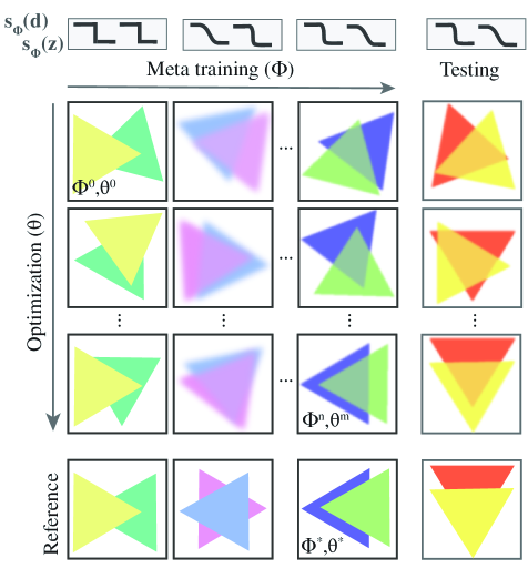
Figure 2: Meta-learning. Meta-optimization consists of two training loops to jointly optimize the scene parameters $\theta$ for one task (vertical) and the renderer parameters $\phi$ across many tasks (horizontal). Each task here is the two triangles that change position to match the reference image shown in the last row. At test time, the optimal renderer is good at solving unseen tasks, shown in the rightmost column. This is, because towards the end of meta-training, the optimization itself got close to the reference. The top shows the soft functions used to render one column: a soft depth step makes the triangles transparent, a soft edge function makes the edges blurry.

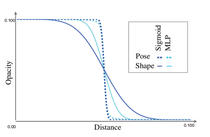
Figure 3: Edge functions for different tasks. Our meta-learning studies two edge functions for $s_{\phi}(d)$ : sigmoid in blue and MLP in cyan. We visualize the meta-learned parameters for two tasks from Figure 5 for optimizing the 2D shape (Logo-1) and the camera pose (cube) by showing the opacity on vertical axis. The same parameters can be used for more complex scenes (i.e. Logo-2 andteapot) without re-meta-training.

mymaths $\mathcal{L}$ mymaths $I_{i}$

Algorithm 1 Meta-learning for Soft Rasterization

1:$\Theta$: Set of task images

2:Meta-learned soft renderer parameter $\phi$

3:$\phi$ = Random

4:for  $i\in[1,n]$ do

5:     $\theta$ = Random

6:     $I_{i}\leftarrow\textsc{SampleImage}(\Theta)$

7:     for  $j\in[1,m]$ do

8:         $\mathcal{L}_{\theta}\leftarrow||\mathcal{R}_{\mathrm{s}}(\theta,\phi)-I_{i}||_{2}$

9:         $\nabla_{\theta}=\textsc{gradient}(\mathcal{L}_{\theta},\theta)$

10:         $\theta=\theta-\lambda_{\theta}\nabla_{\theta}$

11:     end for

12:     $\mathcal{L}_{\phi}\leftarrow||\mathcal{R}_{\mathrm{s}}(\theta,\phi)-I_{i}||_{2}$

13:     $\nabla_{\phi}=\textsc{gradient}(\mathcal{L}_{\phi},\phi)$

14:     $\phi=\phi-\lambda_{\phi}\nabla_{\phi}$

15:end for

3 Meta-learning a differentiable rasterizer

3.1 Meta problem setting

To make systematic progress we move the problem to another level of abstraction. We phrase the challenge as finding a renderer $\mathcal{R}_{\mathrm{s}}$ , parametrized in some way by ${\theta^{\star}_{i}}$, that converges best over a set of tasks ${I_{i}}$:

$$\underset{\mathcal{R}_{\mathrm{s}}}{\operatorname{arg\,min}\ }\mathbb{E}_{i}[||\mathtt{opt}(||\mathcal{R}_{\mathrm{s}}(\theta)-I_{i}||_{2},\theta)-\theta^{\star}_{i}||]\,.$$

In practice, sometimes the ground truth parameters ${\theta^{\star}_{i}}$ are not available but only the images ${I_{i}}$, then the challenge can also be described as:

$$\underset{\mathcal{R}_{\mathrm{s}}}{\operatorname{arg\,min}\ }\mathbb{E}_{i}[||\mathcal{R}_{\mathrm{s}}(\mathtt{opt}(||\mathcal{R}_{\mathrm{s}}(\theta)-I_{i}||_{2},\theta))-I_{i}||]\,.$$

We do not limit ourselves to any discrete set of functions to manually select from, but look into the continuous space of all soft renderers using meta-learning, to be explained now.

3.2 Meta-learning

Meta-Learning is an algorithm for learning to learn and improve the model itself by observing how different models learn. Finn et al. [3] proposed a model-agnostic meta-learning (MAML) algorithm which successfully learns unseen tasks given limited trained samples on a variety of tasks using two training loops. Due to the particularity of our tasks, we use a technique similar to MAML as defined in Alg. 1. MAML proceeds as a nested for loop (L2 and L5). The outer loop optimizes over meta-parameters (in our case, the shape of the softening functions), the inner one over parameters (in our case, the scene parameters). The inner loop is normal gradient descent (L8), with a moderate and fixed number of steps. As such, the inner loop can be rolled out into an expression, that the outer loop can automatically differentiate. The outer gradient update step (L11) then changes the inner optimization parameters, in our case, the differentiable renderer (L12), so that inner the optimization would have gotten closer to its target.

Our solution is not completely an instance of MAML, as in the meta-loop we cannot apply the parameters to a new test instance, which, traditionally, is done in MAML. Another subtle and related difference is, that we do not access the ground truth parameters, we only learn how to reduce the image error, hoping that this will reduce also the parameter error. This is intentional, as it removes the need to supervise with ground-truth parameters and purely relies on images as supervision. Also, we do not meta-train the initializations or step sizes, which, depending on the particular inverse problem at hand, might give additional benefits.

The meta-optimization over all soft rasterizers, parametrized by $\phi$ is:

$$\mathtt{opt}(\mathbb{E}_{i}[||\mathcal{R}_{\mathrm{s}}(\mathtt{opt}(||\mathcal{R}_{\mathrm{s}}(\theta,\phi)-I_{i}||_{2},\theta),\phi)-I_{i}||_{2}],\phi)\,.$$

These parametrized rasterizers do nothing else than a conventional rasterizer, except that when testing the triangle edges or occlusions, they do not use step functions, but a function $s_{\phi}(d)$ that depends on some parameter vector $\phi$ . We will next look into different such parametrized soft edge functions.

3.3 Tunable edge functions

We study two tunable edge functions: sigmoids and MLPs. Different from GenDR [13], we do not, in general, force the softening function to be the Cummulative Density Function (CDF) of another function, because that seems optional and that function would never be required.

Sigmoid:  The function simply is a logistic function with a softening parameter $\phi$

$$s_{\phi}(d)=\operatorname{S}(d)=\frac{1}{1+\exp(-d\cdot\phi)}\,.$$

This function was used already in previous work, where it can be grid-searched due to the low dimensionality. We will see, that a more general class of functions, provides better results:

MLP:  For more general softening, we employ an MLP that comprises five layers with $\tanh$ as internal activations and a residual layer that skips three middle layers, followed by a final sigmoid:

$$s_{\phi}(d)=\operatorname{S}(\mathsf{W}_{5}\tanh(\mathsf{W}_{4}\tanh(\mathsf{W}_{3}\tanh(\mathsf{W}_{2}\tanh(\mathsf{W}_{1}d)))))\,.$$

Network parameters $\mathsf{W}_{1},\ldots,\mathsf{W}_{5}$ of width 4 are initialized randomly from a uniform distribution.

3.4 Tunable occlusion function

Similarly, we also study two tunable functions for $z$-buffering: Softmaxs and MLPs. While in SoftRas [8] the occlusion is addressed using an aggregation in depth along with the output of the edge function, we propose a decoupled approach by learning the softening distribution of the normalized depths for overlapping primitives.

Softmax:  softmax is parametrized by $\phi$ , which can be seen as a multi-dimensional sigmoid function:

$$s_{\phi}(0pt)=\operatorname{\sigma}(0pt)=\frac{\exp(0pt\cdot\phi)}{\sum_{j}{\exp(0pt_{j}\cdot\phi)}}$$

where $j$ is the index of depth buffer.

MLP:  The MLP for softening depth is structured similarly to that of the edge function but replaced tanh with relu and followed by a final softmax:

$$s_{\phi}(0pt)=\operatorname{\sigma}(\mathsf{W}_{5}\mathrm{relu}(\mathsf{W}_{4}\mathrm{relu}(\mathsf{W}_{3}\mathrm{relu}(\mathsf{W}_{2}\mathrm{relu}(\mathsf{W}_{1}0pt)))))\,.$$

Different from the neural aggregation proposed by SoftRas [8], our MLP learns the depth relationship between primitives directly but does not require any features extracted from the images, which is not necessary.

3.5 Combination

Overall, we propose a soft blending in distance $d$ and depth 0ptby meta-learning the $\phi$ for both respectively. We define the final value at pixel $i$ as follows:

$$C_{i}=\sum_{j}s_{\phi_{d}}(d_{j}^{i})\cdot s_{\phi_{z}}(0pt_{j}^{i})\cdot C^{i}_{j}$$

where $s_{\phi_{d}}$ refers to the tunable edge functions, $s_{\phi_{d}}$ refers to the tunable $z$-buffering functions, $C^{i}_{j}$ is the color of pixel $i$ at the $j$-th primitive.

Table 1: Imaged-based and actual errors for three different tasks. Our meta-learning approach for learning an optimized a MLP as well as a Softstep function which is Sigmoid for pose and shape, and Softmax for occlusion task.

Tasks $\rightarrow$	Logo-1	Logo-2	Cube		Teapot		Planes-1		Planes-2
Methods $\downarrow$	Img. err.	Img. err.	Img. err.	Para. err.	Img. err.	Paar. err.	Img. err.	Para. err.	Img. err.	Para. err.
Ours-MLP	$39.50$	$264.47$	$1.84100$	$0.000\,043$	$160.84$	$0.004\,866$	$53.18$	$0.916\,186$	$376.85$	$53.50$
Ours-Soft	$42.39$	$238.42$	$3.00100$	$0.000\,042$	$195.03$	$0.025\,752$	$65.48$	$1.018\,197100$	$310$	$65.94$
SoftRas [8]	$69.86$	$348.22$	$26.11$	$0.001\,832$	$421.88$	$0.749\,609$	$98.92$	$1.421\,160100$	$815.36$	$74.57$
DIB-R [2]	$144.21$	$756.49$	$342.95$	$6.876\,086100$	$835.53$	$6.374\,013100$	$155.17$	$1.744\,660100$	$1132.39$	$70.15$
GenDR [13]	$52.19$	$320.75$	$311.23$	$2.884\,667100$	$763.43$	$7.706\,449100$	$155.17$	$1.744\,660100$	$1132.39$	$70.15$

4 Evaluation

Our evaluation compares different methods (Sec. 4.1) according to different metrics (Sec. 4.2) on different tasks (Sec. 4.3). Results are presented in Sec. 4.5.

4.1 Methods

We compare five different methods, two versions of ours, and three previous approaches. All methods are identical, except for the soft edge handling and use the same rendering with perspective projection, Phong materials under a point light, at the same resolution and no super-sampling.

Ours:  For ours, we study an edge function based on an MLP, denoted as Ours-MLP, and a sigmoid or Softmax function marked as Ours-Softstep.

Previous work:  We compare three published soft edge functions. For previous work, we do not explore their complete system, just the soft edge functions proposed.

SoftRas [8] uses a logistic function with squared absolute part of the distance as their soft edge function:

$$s_{\phi}(d)=\frac{1}{1+\exp(-d\cdot|d|\cdot\phi)}\,,$$

where $\phi$ is fixed to $10^{4}$ in all experiments according to the literature. They also handle occlusion by leveraging aggregation and defining the probabilistic contribution of every primitive. In their aggregation, the weight of foreground color is defined as:

$$s_{\phi}(0pt)=\frac{s_{\phi}(d)\cdot\exp(0pt\cdot\phi)}{\sum_{j}{s_{\phi}(d)\cdot\exp(0pt_{j}\cdot\phi)}+\exp(\epsilon\cdot\phi)}$$

where $\phi$ is also fixed to $10^{4}$ and $s_{\phi}(d)$ here is their logistic function; $\epsilon$ is a small constant.

GenDR by Petersen et al. [13] systematically explores many different edge functions. We choose the gaussian function and gamma function with shape parameter $p=0.5$, which are the best-performer in both optimizing shape and camera pose tasks in their work. In the result section, we only show the best of the two functions. According to the literature, the $\phi$ in shape optimization is grid-searched from $10^{0}$ to $10^{8}$, while in camera pose optimization transitions logarithmically from $10^{1}$ to $10^{7}$. GenDR unlike SoftRas uses hard $z$-buffer in their experiments with probabilistic sum as silhouette aggregation, which can be formulated as:

$$D^{i}=1-\prod_{j}{(1-D_{j}^{i})}.$$

where $D^{i}_{j}$ is the result of $s_{\phi}(d^{i}_{j})$. The lack of softening occlusion functions limits this method for a general and accurate purpose.

DIB-R [2] uses an exponential to map the distance as:

$$s_{\phi}(d)=\exp(-d\cdot\phi)\,.$$

where $\phi$ is set to $1.5\times 10^{4}$ in all experiments. Except in our 2D shape optimization task that they do not include, $\phi=1.5\times 10^{4}$ is infeasible and we set $\phi$ to $10^{-1}$ instead.

Similar to GenDR, this method also does not propose a new technique for softening the depth buffering to handle occlusions but only uses silhouette aggregation.

4.2 Metrics

While we use image distance as a loss, we study two different metrics in our result. The first one is indeed the MSE image metric. The second is the error in parameters. As the optimization is ultimately about discovering these parameters, this additional metric can give further insight into a method’s behavior. Note that we did not use the parameters during learning, only for evaluation.

Image error	Parameter error	Image error	Parameter error
Logo-1 ($a_{1}$)		Logo-2 ($a_{2}$)
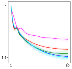
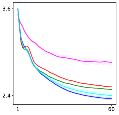
	\begin{overpic}[width=124.21405pt]{images/emp_na2.pdf} \put(48.0,48.0){\small\color[rgb]{0,0,0}} \end{overpic}		\begin{overpic}[width=124.21405pt]{images/emp_na2.pdf} \put(48.0,48.0){\small\color[rgb]{0,0,0}} \end{overpic}
Cube ($b_{1}$)		Teapot ($b_{2}$)
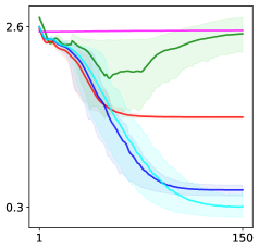
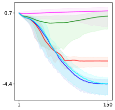
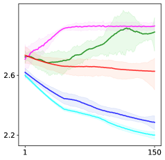
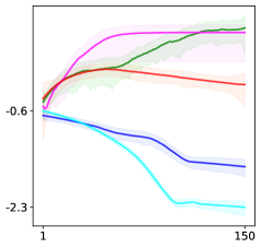
Planes-1 ($c_{1}$)		Planes-2 ($c_{2}$)
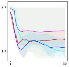
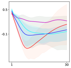
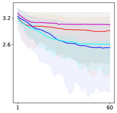
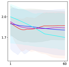
Trained Tasks		Transferred Tasks

Figure 4: Loss (vertical axis, less is better, log scale) at different iterations (horizontal) for four different tasks (rows of plots) according to two metrics (columns of plots). Different methods are shown as color. The solid transparent areas are the 10-90 percentile. As the ground truth parameters are not available for the Shape tasks, no plot is shown there. Our technique performs better than the previous methods ([8, 13, 2] and converges faster with minimum difference to the reference image. The renderings for each iteration is illustrated in Figure 5.

			Ours-MLP	Ours-Softstep	SoftRas [8]	DIB-R [2]	GenDR [13]
Logo-1 ($a_{1}$)		Result
		Error
logo-2 ($a_{2}$)		Result
		Error
Cube ($b_{1}$)		Result
		Error
Teapot ($b_{2}$)		Result
		Error
Planes-1 ($c_{1}$)		Result
		Error
Planes-2 ($c_{2}$)		Result
		Error

Figure 5: Rendering comparisons with previous methods.

4.3 Tasks

We explore three inverse rendering tasks for optimizing shape and camera position, as well as occlusion.

Shape:  In this task, we find the position of hundreds of 2D triangle vertices so as to form a desired target image. The initial triangle positions are randomized. This 2D optimization is similar to the technique proposed by Riso et al. [16] for procedural graphics patterns. We study two variants of the shape task: a trained, and a transfer one.

For the trained variant, a CVF logo is used as the target image during training. The challenge is to ”get back” to the logo.

For the transfer variant, we apply the meta-learned parameters, including both MLP and sigmoid, to a new logo, a CVPR logo. In this case, more initial triangles are optimized to reshape the target.

Pose:  Here, we hold the geometry fixed and optimize the position of the camera, while the up and look-at are fixed. We represent the camera position in spherical coordinates. Again, we study a trained and a transfer condition.

First we set up a simple task rendering a Cube, the initial positions are uniformly randomized as radius $r=5.2$, azimuth $\theta\in[40^{\circ},45^{\circ}]$ and elevation $\varphi\in[50^{\circ},55^{\circ}]$ in each task. The reference positions are also uniformly randomized as $r=4.2$, $\theta\in[80^{\circ},85^{\circ}]$ and $\varphi\in[50^{\circ},55^{\circ}]$.

For transfer experimentation, we replace the cube with a teapot, which has a more complex geometry, thus harder to optimize and not observed during training. The task is repeated for the teapot with $r=1.6$, $\theta\in[42.5^{\circ},45^{\circ}]$ and $\varphi\in[52.5^{\circ},55^{\circ}]$ as initial positions and $r=1.4$, $\theta\in[82.5^{\circ},85^{\circ}]$ $\varphi\in[52.5^{\circ},55^{\circ}]$ as reference positions.

Another way to see the relation in this case, is that the first variant meta-generalizes across pose, while the second meta-generalizes across pose and shape.

The softening functions for these two tasks are visualized in Figure 3 for both of our meta-learned methods.

Occlusion:  We first set three overlapping quadrilaterals with different colors and optimize their depths to arrange them in a correct occlusion order. The depths are uniformly randomized as $z\in[0.5,1.5]$.

Then we again study a transfer condition using eight overlapping quadrilaterals with a larger range of depth as $z\in[-1,3]$, randomized color $C^{3}\in[0,1]$ and randomized center position $x,y\in[-0.3,0.3]$.

As shown in Figure 5 for planes-1, a green quadrilateral and a blue one almost completely cover a red one, which needs to be optimized to the front. Similarly, in planes-2 all eight quadrilaterals need to be successfully ordered in depth same as the reference. The initial order is randomized.

By setting this scenario, we show the accuracy of processing the anteroposterior relationship of different methods directly. When quadrilaterals fully overlap others, hard $z$-buffering and silhouette aggregation will be not enough to handle this problem.

Note that only the $z$ coordinate of each primitive vertex will be optimized with $x$ and $y$ fixed.

4.4 Implementation

We implement the meta-learned soft rasterization to be performed in parallel over all pixels and primitives using JAX [17]. In the rendering, we apply flat shading with Phong materials and back-facing culling in the optimizing and meta-learning. The depth of the background is set to a small constant. All the experiments run on a GTX 1660 SUPER (6G) and we use a meta-learning technique that is similar to classic MAML to learn our meta parameters, which represent the softness of different distributions both in 2D and depth space. The full algorithm is outlined in Alg. 1. We use Adam as the optimizer for both the meta parameters as well as the scene parameters of tasks ($\beta_{1}=0.9,\beta_{2}=0.999,\epsilon=10^{-8}$, learning rate $=0.1$.) The loss of optimizing both the scene parameters and meta parameters is image MSE between a reference image and a rendering result. Note that the optimization is not supervised by the ground truth parameters at any point.

In the shape and pose tasks, we apply our meta-learned softmax to solve the occlusion problem and also apply the probabilistic sum for silhouette aggregation for all methods. In the shape task, all primitives are in the same depth, thus the overlapping pixels are equally weighted. In the occlusion task, we choose square-root of logistic as the soft edge function for all methods.

4.5 Results

Quantitative:  Quantitative results are seen in Figure 4. Here we analyze all tasks according to all metrics using all methods. A successful method will —according to both metrics— have a graph that quickly and reliably goes to a low (preferable) error value; and also stays down. Further, a strong method would be consistent, i.e., not have percentiles with undesired outliers (narrow funnel).

We see that across the tasks, and consistent between metrics, Our-MLP performs best (cyan), followed by a meta-tuned Our-softstep (blue). This is true both for the end point (right in each plot), as for most (interruptible) in-between iterations as well. For some iterations (horizontal axis in each plot), all methods perform similarly in most tasks and for both metrics, but eventually, meta-learned methods take a lead while others plateau. In some examples, existing methods could not solve the task with the published default values at all, while ours can adapt to any task on any scale. We also see, that while our work optimizes the image error, the ultimate currency is the parameter error, our metric, which also is the lowest for us.

For occlusion, all methods start to get worse towards the end, both in image and parameter error, but our two methods still come out strongest. We also can see, that the transfer from learning on one task and testing on another one can succeed, by comparing the first and the second pair of rows, in which the first task class is seen in meta-training, while the second one of the pair is not. This shows the potential to save computational resources on optimizing complex tasks by training on related simpler ones.

Qualitative:  Similarly, the qualitative results of the same tasks are illustrated in Figure 5 comparing the renderings of the final iteration from Figure 4. As shown in the Error results, Our-MLP performs best followed by the meta-learned Our-softstep among all methods. The animated results of the convergence of these results are provided in the supplementary materials.

For shape and pose tasks, our results reproduce the closest to the reference compared to the previous works starting from the same initialization. And the successful transfer of the meta parameters from one task to another can be seen in each pair of rows.

For occlusion, DIB-R and GenDR methods do not soften depth buffering and only SoftRas is comparable with our methods in which theirs also underperforms. Because their occlusion softening function works in tandem with their edge softening while our methods decouple these two and hence perform slightly more accurately.

5 Conclusion

We have presented the use of meta-learning to learn from a continuous space of the softening operations to soften edges and occlusion functions and enable differentiable rendering. To this end, we study two tunable functions (sigmoid and MLPs as edge functions and similarly softmax and MLPs as occlusion functions) and jointly optimize over their parameters as well as the scene parameters to address the issue of discontinuity. The softening in the 2D space enables optimizing shape and pose. The softening in the depth space allows resolving occlusion using differentiable rendering. We have also explored the generalization ability of meta-learned softening operations, which reveals the potential power of our method for handling complex problems.

In future work, we would like to apply this technique for more general tasks as well as dynamic optimization to switch between the softening functions for the best performance. Intuitively, in the early stage of optimization, smoother functions can be deployed to capture the low frequencies while details are optimized later using a different softening function. Besides, when rendering different models and scenes the softening functions can also be switched to the optimal correspondingly. Moreover, this technique can be further improved by using the neural representation or neural proxy methods to provide heuristic gradients for the rasterization instead of analytical approaches as explored in this work.

References

- Chen et al. [2019] Wenzheng Chen, Huan Ling, Jun Gao, Edward Smith, Jaakko Lehtinen, Alec Jacobson, and Sanja Fidler. Learning to predict 3d objects with an interpolation-based differentiable renderer. In H. Wallach, H. Larochelle, A. Beygelzimer, F. d'Alché-Buc, E. Fox, and R. Garnett, editors, Advances in Neural Information Processing Systems, volume 32. Curran Associates, Inc., 2019.
- Chen et al. [2021] Wenzheng Chen, Joey Litalien, Jun Gao, Zian Wang, Clement Fuji Tsang, Sameh Khamis, Or Litany, and Sanja Fidler. Dib-r++: Learning to predict lighting and material with a hybrid differentiable renderer, 2021.
- Finn et al. [2017] Chelsea Finn, Pieter Abbeel, and Sergey Levine. Model-agnostic meta-learning for fast adaptation of deep networks, 2017.
- Gupta et al. [2020] Anshul Gupta, Joydeep Medhi, Aratrik Chattopadhyay, and Vikram Gupta. End-to-end differentiable 6dof object pose estimation with local and global constraints, 2020.
- Kato et al. [2018] Hiroharu Kato, Yoshitaka Ushiku, and Tatsuya Harada. Neural 3d mesh renderer. In Proc. CVPR, pages 3907–3916. Computer Vision Foundation / IEEE Computer Society, 2018. doi: 10.1109/CVPR.2018.00411.
- Kato et al. [2020] Hiroharu Kato, Deniz Beker, Mihai Morariu, Takahiro Ando, Toru Matsuoka, Wadim Kehl, and Adrien Gaidon. Differentiable rendering: A survey, 2020.
- Li et al. [2018] Tzu-Mao Li, Miika Aittala, Frédo Durand, and Jaakko Lehtinen. Differentiable monte carlo ray tracing through edge sampling. 37(6), 2018.
- Liu et al. [2019] Shichen Liu, Tianye Li, Weikai Chen, and Hao Li. Soft rasterizer: A differentiable renderer for image-based 3d reasoning. In Proceedings of the IEEE/CVF International Conference on Computer Vision, pages 7708–7717, 2019.
- Loper and Black [2014] Matthew M. Loper and Michael J. Black. Opendr: An approximate differentiable renderer. In David Fleet, Tomas Pajdla, Bernt Schiele, and Tinne Tuytelaars, editors, Computer Vision – ECCV 2014, pages 154–169, Cham, 2014. Springer International Publishing.
- Nimier-David et al. [2021] Merlin Nimier-David, Zhao Dong, Wenzel Jakob, and Anton Kaplanyan. Material and lighting reconstruction for complex indoor scenes with texture-space differentiable rendering. In Adrien Bousseau and Morgan McGuire, editors, 32nd Eurographics Symposium on Rendering, EGSR 2021 - Digital Library Only Track, Saarbrücken, Germany, June 29 - July 2, 2021, pages 73–84. Eurographics Association, 2021. ISBN 978-3-03868-157-1.
- Petersen et al. [2019] Felix Petersen, Amit H. Bermano, Oliver Deussen, and Daniel Cohen-Or. Pix2vex: Image-to-geometry reconstruction using a smooth differentiable renderer. CoRR, abs/1903.11149, 2019.
- Petersen et al. [2021] Felix Petersen, Christian Borgelt, Hilde Kuehne, and Oliver Deussen. Learning with algorithmic supervision via continuous relaxations. In A. Beygelzimer, Y. Dauphin, P. Liang, and J. Wortman Vaughan, editors, Advances in Neural Information Processing Systems, 2021.
- Petersen et al. [2022] Felix Petersen, Bastian Goldluecke, Christian Borgelt, and Oliver Deussen. Gendr: A generalized differentiable renderer. In Proceedings of the IEEE/CVF Conference on Computer Vision and Pattern Recognition (CVPR), pages 4002–4011, June 2022.
- Pineda [1988] Juan Pineda. A parallel algorithm for polygon rasterization. Proceedings of the 15th annual conference on Computer graphics and interactive techniques, 1988.
- Rhodin et al. [2015] Helge Rhodin, Nadia Robertini, Christian Richardt, Hans-Peter Seidel, and Christian Theobalt. A versatile scene model with differentiable visibility applied to generative pose estimation. 2015 IEEE International Conference on Computer Vision (ICCV), pages 765–773, 2015.
- Riso et al. [2022] Marzia Riso, Davide Sforza, and Fabio Pellacini. pop: Parameter optimization of differentiable vector patterns. Computer Graphics Forum, 41(4):161–168, 2022.
- Schoenholz and Cubuk [2020] Samuel S. Schoenholz and Ekin D. Cubuk. Jax m.d. a framework for differentiable physics. In Advances in Neural Information Processing Systems, volume 33. Curran Associates, Inc., 2020.
- Zhang et al. [2020] Cheng Zhang, Bailey Miller, Kai Yan, Ioannis Gkioulekas, and Shuang Zhao. Path-space differentiable rendering. ACM Trans. Graph., 39(4), aug 2020.