Quantum theories with local information flow

Abstract

Bell non-locality is a term that applies to specific modifications and interpretations of quantum mechanics. Yet Bell’s original 1964 theorem is often used to assert that unmodified quantum mechanics itself is non-local and that local realist interpretations are untenable. Motivated by Bell’s original inequality, we identify four viable categories of quantum theories: local quantum mechanics, superdeterminism, non-local collapse quantum mechanics, and non-local hidden variable theories. These categories, however, are not restricted by Bell’s definition of locality. In light of currently available no-go theorems, local and deterministic descriptions seem to have been overlooked, and one possible reason for that could be the conflation between Bell-locality and a broader principle of locality. We present examples of theories where a local flow of quantum information is possible and assess whether current experimental proposals and an improved philosophy of science can contrast interpretations and distinguish between them.

1 Introduction

John Bell published his celebrated inequality in 1964 bell64 . Its implications remain eagerly discussed to this day bell64 ; bell_2004 ; Bertlmann2017 . The derivation of the inequality is simple, but its meaning has a history of misunderstandings Maudlin2014 . Perhaps for the first time after the development of quantum mechanics, and the proliferation of the first interpretations, one was able to rule out a large category of quantum interpretations, namely: local hidden variable theories admitting statistical independence. Bell showed that the field of foundations of quantum mechanics is not to be restricted to philosophy only, but that physics also has its part in this endeavour bell_2004 ; Bertlmann2017 ; Nurgalieva2020 . Based on Bell’s result, one then hopes to develop refined no-go theorems and contrast viable categories of interpretations with constraints imposed by both quantum field theory and general relativity to narrow down the menu of interpretations Myrvold2021 ; Clauser1969 ; Pusey2012 ; Frauchiger2018 .

Recently, a new wave of no-go theorems involving thought experiments Frauchiger2018 ; Nurgalieva2020 ; Nurgalieva2022 ; Bertlmann2017 , developments in the theory of decoherence and quantum computing Schlosshauer2007 , and prizes awarded to the foundations of quantum mechanics reignited the interest in interpretational issues. Even orthodox philosophical stances are undergoing revisions Bertlmann2017 . However, half a century after Bell’s paper bell64 , his results are advertised in favour of non-local formulations of quantum mechanics Larsson2014 ; Maudlin2014 ; Hance2022nature , as if there were no other alternatives, even if they predict possible experimental tests Hossenfelder2011 ; Carroll2021 . For a recent rebuttal to quantum non-locality, see Ref. Hance2022nature .

Motivated by the apparent unjustified conclusion that Bell’s 1964 theorem necessarily leads to quantum non-locality, we analyse four viable categories of theories: local quantum mechanics, superdeterminism, non-local collapse quantum mechanics, and non-local hidden variable theories. We find that even in explicitly non-local hidden variable theories such as Bohmian mechanics, a local flow of quantum information is possible. We discuss three examples of theories in categories that admit such a local information flow, namely: the superdeterministic $\psi$-ensemble interpretation, Bohmian mechanics, and Everettian mechanics. We then argue that it seems unfitting to use Bell’s theorem to discard local and deterministic theories.

In Sec. 2 we review Bell’s original 1964 theorem and establish four viable categories of quantum theories. These categories remain valid even in light of more contemporary no-go theorems. In Sec. 3, we differentiate between the broader principle of locality and the more restrictive form of Bell-locality. Then, we present one example from each of the three categories admitting a local information flow. We show that the local flow of quantum information is especially transparent in the Heisenberg picture. In Sec. 4, we contrast the categories and, based on recent developments, evaluate the prospect of distinguishing categories of interpretations defending deterministic and local options. We conclude by using Deutsch’s philosophy of science Deutsch2016 to contrast superdeterministic and Everettian-type theories.

We will soon review that certain extensions of quantum mechanics are constrained by Bell’s original inequality. Non-extended quantum mechanics violates Bell’s inequality. In this paper, we refer to interpretations of quantum mechanics as non-extended theories, even though experimental tests and philosophical views may distinguish between interpretations. Different interpretations might postulate the Born rule as part of quantum mechanics or derive it within unitary quantum mechanics. We consider theories that introduce hidden variables or non-unitary physical processes as extensions of quantum mechanics.

2 Categories of quantum theories

Bell’s original 1964 theorem belongs now to a collection of no-go theorems commonly referred to as Bell’s theorems. Early versions impose restrictions on modifications of quantum mechanics only, whereas later updates also restrict quantum mechanics itself Myrvold2021 . For categorisation purposes, in this section, we consider Bell’s original 1964 theorem bell64 that sets restrictions on hidden variable theories. Even if they are defined following the original inequality, the categories remain valid even when considering a broader principle of locality. In what follows, we briefly recollect Bell’s original result.

2.1 Bell’s 1964 inequality

A pair of identical particles $A$ and $B$ evolve into the entangled spin-singlet state $|\psi\rangle=(|\uparrow\downarrow\rangle-|\downarrow\uparrow\rangle)/\sqrt{2}$ through local interactions. Particle $A$ moves to lab $L_{A}$, and particle $B$ to lab $L_{B}$. Labs $L_{A}$ and $L_{B}$ occupy space-like separated regions. The unit vector $\mathbf{a}$ sets up the reference frame (or the detector setting) of lab $L_{A}$ to measure the spin observable $\boldsymbol{\sigma}$ of particle $A$. Similarly, $\mathbf{b}$ sets up $L_{B}$. Therefore, the setups at $L_{A}$ and $L_{B}$ measure the observables $\boldsymbol{\sigma}\cdot\mathbf{a}$ and $\boldsymbol{\sigma}\cdot\mathbf{b}$, respectively. Bell calls the respective eigenvalues $A(\mathbf{a})=\pm 1$ and $B(\mathbf{b})=\pm 1$. The quantum mechanical expectation value for the entangled state $|\psi\rangle$ of the product of the observables at different labs is

$$P(\mathbf{a},\mathbf{b})=\langle\psi|(\boldsymbol{\sigma}\cdot\mathbf{a})(\boldsymbol{\sigma}\cdot\mathbf{b})|\psi\rangle=-\mathbf{a}\cdot\mathbf{b},$$ (1)

which shows that the expectation value depends on the detector settings. So far, there is no mention of hidden variables. A virtue of Eq. (1) is that $P(\mathbf{a},\mathbf{b})$ does not depend on whether one is working in the Schrödinger or Heisenberg picture.

One usually refers to quantum mechanics as the combination of an equation of motion, such as the Schrödinger equation or the Heisenberg equation of motion, along with the Born rule Eq. (1) to calculate expectation values. The calculation of expectation values via the Born rule is uncontroversial, but its meaning depends on a particular interpretation. For instance, the Copenhagen interpretation asserts that a measurement triggers a random collapse, and the outcome probability is postulated as the Born rule. On the other hand, unitary interpretations of quantum mechanics do not postulate the Born rule but seek to explain it instead Deutsch1999 ; Zurek2009 ; Marletto2016 ; Sebens2018 ; Lazarovici2020 .

Now, Bell guides us to modify quantum mechanics by assuming a set of local hidden variables $\lambda$, which compile all the necessary information to supposedly complete quantum mechanics. The variables now affect the eigenvalues $A(\mathbf{a},\lambda)$ and $B(\mathbf{b},\lambda)$. The writing of $A(\mathbf{a},\lambda)$ and $B(\mathbf{b},\lambda)$ contains an implicit assumption: the eigenvalue $A(\mathbf{a},\lambda)$ at lab $L_{A}$ does not depend on $\mathbf{b}$. Similarly, $B(\mathbf{b},\lambda)$ does not depend on $\mathbf{a}$. Then, Bell assumes that the hidden variable dependent expectation value can be calculated using bell64

$$P_{H}(\mathbf{a},\mathbf{b})=\int\mathrm{d}\lambda\,\rho(\lambda)A(\mathbf{a},\lambda)B(\mathbf{b},\lambda),$$ (2)

where $\rho(\lambda)$ is a normalised hidden variable distribution. By writing Eq. (2), Bell excluded the possibility of superdeterminism, for which the probability distribution $\rho(\mathbf{a},\mathbf{b},\lambda)\neq\rho(\lambda)$ Wharton2020 ; Hossenfelder2020 ; Hossenfelder2020_perplexed ; Hance2022 .

If Bell’s type local hidden variable theory is to reproduce quantum mechanics, then one expects $P_{H}(\mathbf{a},\mathbf{b})=P(\mathbf{a},\mathbf{b})$. But within the assumptions of Bell hidden variable locality and statistical independence, this is generally not possible. Using simple manipulations bell64 , Bell showed that $P_{H}(\mathbf{a},\mathbf{b})$ must satisfy the inequality

$$1+P_{H}(\mathbf{b},\mathbf{c})\geq\left|P_{H}(\mathbf{a,\mathbf{b}})-P_{H}(\mathbf{a,\mathbf{c}})\right|,$$ (3)

which today bears his name. By using the quantum mechanical expectation value $P(\mathbf{a},\mathbf{b})$ instead of the hidden variable expectation value $P_{H}(\mathbf{a},\mathbf{b})$ in Eq. (3), it is easy to produce special cases where $P(\mathbf{a},\mathbf{b})$ – usually, simply referred to as quantum mechanics – violates the inequality. Therefore, Bell’s original theorem in Ref. bell64 states that statistical predictions of quantum mechanics are incompatible with local hidden variable formulations that obey statistical independence. Hidden variable no-go theorems such as Eq. (3) impose restrictions on modifications of quantum mechanics, not on quantum mechanics itself. Therefore, such theorems impose no restrictions on quantum mechanics itself, which can still be local according to other principles. We will mention such a local description in Sec. 3.5.

2.2 Categories

Bell’s 1964 results summarised in the previous section exclude the possibility of a local hidden variable theory admitting statistical independence. That being the case, quantum theories (extended or not) might still be:

1. Local quantum mechanics without hidden variables. This includes unitary quantum interpretations Everett1957 ; Brown2019 ; Kuypers2021 ; Rovelli1996 ; MartinDussaud2019 ; Zurek2009 ; Gambini2018 or information approaches such as Qubism Fuchs2013 ; Fuchs2014 ;

2. Local hidden variable extensions of quantum mechanics that violate statistical independence, that is, superdeterminism Hance2022 ; tHooft2016 ; Sen2022 ;

3. Non-local quantum mechanics without hidden variables. In these interpretations, a collapse Faye2019 ; Ghirardi1986 ; Bassi2013 or handshake Cramer1986 ; Kastner2017 implements non-locality;

4. Non-local hidden variable extensions of quantum mechanics. The most prominent example is Bohmian mechanics bohm1952 .

	No hidden variables	Hidden variables
Local	(A) Unitary quantum mechanics Everettian quantum mechanics Everett1957 ; Brown2019 ; Kuypers2021 Relational quantum mechanics Rovelli1996 ; MartinDussaud2019 Quantum Darwinism Zurek2009 Montevideo interpretation Gambini2018 Information approaches*Fuchs2013 ; Fuchs2014	(B) Superdeterminism $\Psi$-ensemble interpretation Hance2022 Cellular Automaton tHooft2016 Invariant set theory Sen2022
Non-local	(C) Collapse or handshake Copenhagen interpretations Faye2019 Objective-collapse theories Ghirardi1986 ; Bassi2013 Transactional interpretation Cramer1986 ; Kastner2017	(D) Non-local hidden variables Bohmian mechanics bohm1952

Table 1: Categories of viable quantum theories with some examples. (A) Local quantum interpretations. The asterisk indicates that information approaches might be unitary or non-unitary. (B) Superdeterministic theories. (C) Collapse or handshake interpretations. (D) Non-local hidden variable theories. Categories (B) and (D) are extensions of quantum mechanics.

Based on surveys on interpretations of quantum mechanics Schlosshauer2013 ; Sivasundaram2016 ; Nurgalieva2020 , in Tab. 1, we distribute a sample of theories according to the four categories. We scanned the literature for recent developments related to Bell’s inequality with interpretive claims, either explicit or implicit; see Ref. Myrvold2021 and Refs. therein. We noticed the following trend: the possibility of Bohmian mechanics (D) is usually recognised and either embraced Lazarovici2020 , or rejected based on arguments beyond Bell’s theorem. The possibility of superdeterminism (B) is frequently overlooked or rejected on philosophical grounds Larsson2014 ; Maudlin2014 . Yet a resurgence in superdeterminism is undergoing Hossenfelder2011 ; Hossenfelder2020_perplexed ; Hossenfelder2020 ; Hance2022 ; tHooft2016 . Rejecting hidden variables completely, current literature typically falls back to collapse interpretations (C), declaring that quantum mechanics must be intrinsically non-local gottfried2004 ; Brunner2014 . However, while collapse-type interpretations are popular ways of violating Bell’s inequality, Tab. 1 also shows a category of local quantum mechanical interpretations (A), which also violate Bell’s inequality.

2.3 No-go theorems

To our knowledge, the categories outlined in Tab. 1 withstand not only Bell’s 1964 hidden variable theorem but also more contemporary no-go theorems. Let us mention some of them.

Later Bell theorems (see Refs. bell_2004 ; Myrvold2021 ) assume local determinism and causality to constrain not only hidden variable theories but also quantum mechanics itself. In Sec. 3.1, we clarify how categories (A) and (B) persist despite these constraints. Other noteworthy no-go theorems include the CHSH theorem Clauser1969 , the Pusey-Barrett-Rudolph theorem Pusey2012 , and the Frauchiger-Renner no-go theorem Frauchiger2018 .

Our purpose here, however, is not to defend the feasibility of each of the aforementioned quantum theories by analysing how each one of them survives the most recent no-go theorems. For this, the reader might consult the specific references in Tab. 1. In this paper, we simply argue that Bell’s 1964 no-go theorem of Ref. bell64 , as habitually used to advertise quantum non-locality, actually imposes no restrictions on category (A).

In the following section, we discuss the examples of the $\Psi$-ensemble interpretation, Bohmian mechanics and Everettian mechanics. Although these theories belong to different categories, they are all deterministic and admit a local information flow - a concept which was first introduced in Ref. Deutsch2000 . At the end, we assess whether these interpretations are expected to be distinguishable in the philosophical domain only.

3 Local information flow

A local flow of information refers to the process of carrying information from one location to another through local interactions, as stated in Ref. Deutsch2000 . For a deeper discussion on the definition of information and its relation with physical laws, we refer the reader to Ref. Deutsch2015 .

This section is motivated by the following problem: suppose that first two systems $A$ and $B$ interact with each other and become entangled, and then are sent to space-like separated regions. After this, system $B$ gets entangled with a third system $C$. Although $A$ and $C$ never interacted with each other, they are now entangled.

Is this a non-local effect? We show that within superdeterminism, Bohmian mechanics and Everettian mechanics, the answer is no.

3.1 Definitions

According to Raymond-Robichaud RaymondRobichaud2021 , local realism is summarised by the following principles:

(i) There is a real-world; (ii) It can be decomposed into various parts, called systems; (iii) A system may be decomposed into subsystems; (iv) Every system is a subsystem of the global system consisting of the entire world; (v) At any given time, each system is in some state; (vi) The state of a system determines, and is determined by, the state of its subsystems; (vii) What is observable in a system is determined by the state of the system; (viii) The state of the world evolves according to some law; (ix) The evolution of the state of a system can only be influenced by the state of systems in its local neighbourhood.

We refrain from assessing whether this is a good definition of local realism or not, but we do use it to clarify what in this paper is meant by a local theory.

Applied to relativity, this definition implies that an action performed at some point cannot affect another point faster than the speed of light. Yet when applied to quantum mechanics, the above definition does not imply that local theories must be described by hidden variables.

While this definition of locality may appear conservative, it should be noted that it is not equivalent to the assumptions of Bell-locality. In Bell’s seminal The Theory of Local Beables bell_2004 , he demonstrates that quantum mechanics cannot be described as locally causal when implicitly assuming that measurements yield single outcomes. This results in a more stringent interpretation of local causality, in which quantum mechanics is indeed not locally causal according to Bell’s criteria.

However, if one is open to relaxing the assumption of single outcomes, then according to Raymond-Robichaud’s definition, quantum mechanics can be considered local and compatible with the principles of relativity. Consequently, it is possible to discuss local, deterministic, and causal theories that do not adhere to Bell-locality, such as the ones listed in categories (A) and (B) of Tab. 1. The categorisation refers to a broader concept of local causality such as Raymond-Robichaud’s and not to Bell-locality. Then, in the context of a local theory, one can explore how information encoded in physical states flows within causally connected local regions.

3.2 The $\psi$-ensemble interpretation

Superdeterminism is not usually considered an interpretation of quantum mechanics. Instead, it is a more fundamental deterministic theory than quantum mechanics. A particular implementation of superdeterminism, the $\psi$-ensemble interpretation Hance2022 , is a $\psi$-epistemic theory in the sense that the wavefunction emerges from more fundamental hidden variable constituents. The distinctive property of superdeterministic theories is that they violate statistical independence, that is, they hold $\rho(\mathbf{a},\mathbf{b},\lambda)\neq\rho(\lambda)$ Wharton2020 ; Hossenfelder2020 ; Hossenfelder2020_perplexed ; Hance2022 . Therefore, the derivations leading to the Bell’s inequality in Eq. (3) do not apply. A superdeterministic expectation value is exempt from violating Bell-type inequalities. Technology permitting, expectation values that satisfy Eq. (3) could experimentally favour superdeterminism.

Let us adopt the hidden variables collectively described by $\kappa(t)$ as presented in the $\psi$-ensemble interpretation Hance2022 . We denote the hidden variables by $\kappa(t)$ (just as in Ref. Hance2022 ), because they are slightly less general than Bell’s hidden variables $\lambda(t)$. The difference does not concern us here. The $\kappa(t)$ determine the outcomes at the time of measurement. For the pair of particles in the Bell test, the two possible outcomes are specified in the state $|\psi\rangle=(|\uparrow\downarrow\rangle-|\downarrow\uparrow\rangle)/\sqrt{2}$. Let us denote the cluster of hidden variables leading to the outcome $|\uparrow\downarrow\rangle$ as $\{\kappa\}_{\uparrow\downarrow}$, and $\{\kappa\}_{\downarrow\uparrow}$ to $|\downarrow\uparrow\rangle$. The hidden variables deterministically map to a definite measurement outcome at the time of measurement. This is how superdeterminism solves the problem of outcomes Schlosshauer2007 . Observing the state $|\uparrow\downarrow\rangle$ reveals information (through the mapping) about the value of the hidden variable at the time of measurement. These hidden variables are causally local because the information about the settings $(\mathbf{a},\mathbf{b})$ was already available at the time the entangled state was prepared through local interactions.

Because the $\psi$-ensemble interpretation has more elements than quantum mechanics, predictions other than standard quantum mechanics are theoretically possible. In standard quantum mechanics, an ensemble of identically prepared states will generally admit different outcomes. In the $\psi$-ensemble interpretation, they are actually not identical, because they had different hidden variable values that originated different outcomes. One could then think of situations between consecutive measurements for which standard quantum mechanics predicts different results between measurements, but in which, in the $\psi$-ensemble interpretation, the hidden variables would not have time to change their cluster. Therefore, superdeterminism could be testable in situations where the hidden variables do not change between measurements. The details of such an experimental proposal can be found in Refs. Hossenfelder2011 ; Hossenfelder2014 .

Some of the most common objections raised against superdeterminism include conspiracy arguments and more recently cosmic Bell tests Rauch2018 . Responses to these objections can be found in Ref. Hossenfelder2020 . This is an ongoing discussion that we do not further address here.

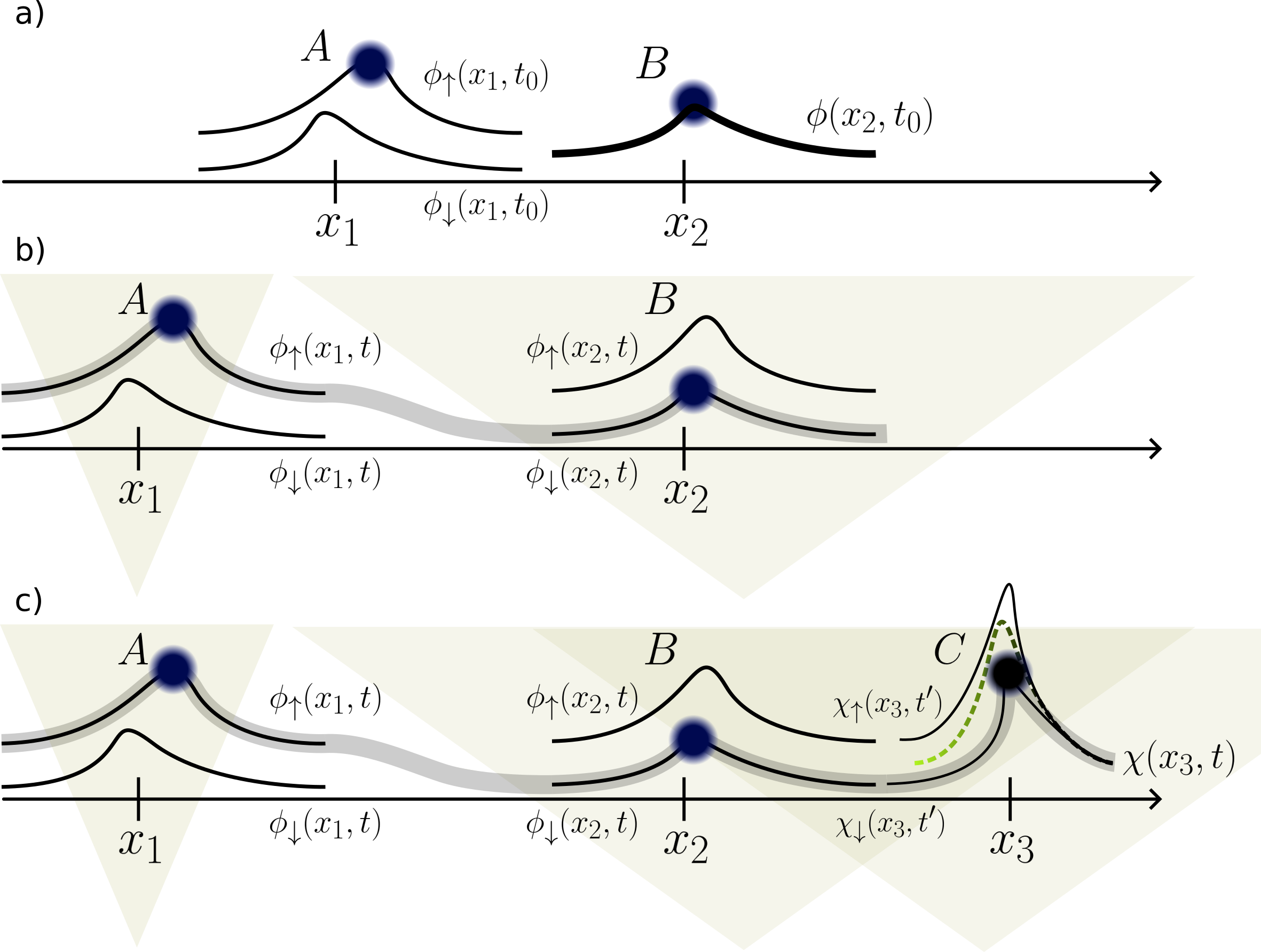
Figure 1: The entangling of three particles $A$, $B$ and $C$ through local interactions. Here $t^{\prime}>t>t_{0}$. (a) $A$ and $B$ are initially unentangled. (b)Entanglement through local interactions sets up the relative states $\phi_{\uparrow}(x_{1},t)\phi_{\downarrow}(x_{2},t)$ and $\phi_{\downarrow}(x_{1},t)\phi_{\uparrow}(x_{2},t)$. The particles illustrated by blue disks move to space-like separated regions indicated by the shaded triangles. (c) Meiosis of the measurer $C$. The detector $C$ verifies the $B$ particle’s spin eigenvalue by interacting with it in the space-like intersecting region. From $t$ to $t^{\prime}$, the only new foliation occurs in the measurer within the space-like intersecting region. The dashed line indicates the unfoliated detector $C$ at time $t$, and the two thinner solid lines show the two new foliations joining the already foliated entangled state. The new spatially extended preferred foliation $\phi_{\uparrow}(x_{1},t^{\prime})\phi_{\downarrow}(x_{2},t^{\prime})\chi_{\downarrow}(x_{3},t^{\prime})$ is shown as the thick grey line.

3.3 Bohmian mechanics

If one seeks a hidden variable theory enjoying statistical independence, then Bell’s 1964 theorem constrains the theory to have elements with action between space-like separated regions. The most prominent example is Bohmian mechanics bohm1952 ; Maudlin2019 ; Lazarovici2020 .

The ontology of Bohmian mechanics is straightforward: there is a pilot-wave $\Psi$ that evolves according to the Schrödinger equation in coordinate space

$$i\hbar\frac{\partial}{\partial t}\Psi(\mathbf{r}_{1},\mathbf{r}_{2},\ldots,\mathbf{r}_{N}\mathchar 24635\relax\;t)=\hat{H}\Psi(\mathbf{r}_{1},\mathbf{r}_{2},\ldots,\mathbf{r}_{N}\mathchar 24635\relax\;t).$$ (4)

The field $\Psi$ pilots $N$ particles, which are also part of the ontology. Each particle $i$ moves according to its guiding equation,

$$m_{i}\frac{\mathrm{d}\mathbf{R}_{i}}{\mathrm{d}t}=\hbar\,\mathrm{Im}\nabla_{i}\ln\Psi.$$ (5)

The solution of Eq. (5) determines each particle’s Bohmian trajectory $\mathbf{R}_{i}(t)$. Finding the set of all trajectories $\{\mathbf{R}_{i}(t)\}$ is a formidable task; yet unnecessary for practical purposes. Similarly to classical statistical mechanics, the collective properties can be obtained from typicality arguments, even though the microstate $\{\mathbf{R}_{i}(t),m_{i}\frac{\mathrm{d}\mathbf{R}_{i}}{\mathrm{d}t}\}$ remains unknown Lazarovici2020 .

Let us now describe the entangled spin-singlet state $|\psi\rangle$ in the context of Bohmian mechanics. The pilot-wave evolves autonomously according to Eq. (4). At time $t_{0}$, the two-particle field is separable:

$$\Psi(x_{1},x_{2}\mathchar 24635\relax\;t_{0})=\langle x_{1},x_{2}|\psi(t_{0})\rangle=\frac{1}{\sqrt{2}}\left[\phi_{\uparrow}(x_{1},t_{0})+\phi_{\downarrow}(x_{1},t_{0})\right]\phi(x_{2},t_{0}).$$ (6)

Next, the positions $x_{1}$ and $x_{2}$ are close enough for the particles $A$ and $B$ to interact. The local interaction is such that the field evolves to the entangled singlet state

$$\Psi(x_{1},x_{2}\mathchar 24635\relax\;t)=\frac{1}{\sqrt{2}}\left[\underline{\phi_{\uparrow}(x_{1},t)\phi_{\downarrow}(x_{2},t)}-\phi_{\downarrow}(x_{1},t)\phi_{\uparrow}(x_{2},t)\right].$$ (7)

The underlined term will be explained shortly. Figs. 1(a,b) illustrate the evolution of the position-dependent wave-packets in Eqs. (6) and (7). We know that particle $A$ is in position $X_{A}(t)$ at lab $L_{A}$, and particle $B$ is in position $X_{B}(t)$ at lab $L_{B}$. The particles’ positions are indicated by the blue disks in Fig. 1. The positions are determined by their respective guiding equations. For the particle at lab $L_{A}$, we have

$$m_{A}\frac{\mathrm{d}X_{A}}{\mathrm{d}t}=\hbar\,\mathrm{Im}\frac{\partial}{\partial x_{1}}\ln\Psi\left(x_{1},X_{B}(t),t\right)\bigr{|}_{x_{1}=X_{A}(t)}.$$ (8)

The spin-singlet state ensures two possibilities:

1. The field $\phi_{\uparrow}(x_{1},t)$ pilots the particle $A$ and the field $\phi_{\downarrow}(x_{2},t)$ pilots the particle $B$;

2. The field $\phi_{\downarrow}(x_{1},t)$ pilots the particle $A$ and $\phi_{\uparrow}(x_{2},t)$ pilots the particle $B$.

These two options accessible to the particles determine the relative states $\phi_{\uparrow}(x_{1},t)\phi_{\downarrow}(x_{2},t)$ and $\phi_{\downarrow}(x_{1},t)\phi_{\uparrow}(x_{2},t)$ in Eq. (7); see Fig. 1(b). The initial conditions of the Bohmian system determine which relative state the particles populate. Without loss of generality, we assume possibility one, which corresponds to the occupation of the underlined relative state in Eq. (7). Also, from Eq. (8) we see that the particle at $X_{A}$ likely accommodates ($\frac{\mathrm{d}X_{A}}{\mathrm{d}t}\approx 0$) where the derivative of the logarithm is zero, which happens when $\phi_{\uparrow}(x_{1},t)$ is extreme; as shown in Fig. 1.

Since the particles occupy the underlined relative state in Eq. (7), one frequently labels it as the preferred foliation of the entangled state Durr2014 ; Kuypers2021 . The second empty foliation could have been the preferred one if the initial conditions were different, or could still evolve to be the preferred foliation if populated in the future.

Due to the guiding Eq. (8) (the particles), Bohmian mechanics is non-local. The trajectory $X_{A}(t)$ depends on the global pilot-wave $\Psi$, which includes field deformations that occur in space-like separated regions. Yet a frequently underappreciated property of pilot-waves is that fields of subsystems $\phi_{\uparrow(\downarrow)}(x,t)$ only interfere locally. This was also pointed out in Ref. Tipler2014 in the context of Everettian mechanics. As long as the information is processed by the pilot-wave, a local information flow is possible, even in a theory with non-local elements. In quantum information circuits, quantum information processing occurs via entanglement and interference effects Nielsen2010 , which are properties of the pilot-wave. For this reason, in Bohmian mechanics, although the particles make up the computing device, the information flows through the pilot-wave. In Sec. (3.5), we will show how the information flows, which can be understood both in a pilot-wave (Schrödinger) Tipler2014 , and even better in the Heisenberg picture Deutsch2000 .

We now consider a third subsystem $C$ with its wave $\chi(x_{3},t)$ guiding its particle (or collection of particles), that will act as the measurer of the particle at lab $L_{B}$. In Fig. 1(c), $\chi(x_{3},t)$ is represented by the dashed line. The measurer $C$ is sufficiently close to interact with $B$, but not with $A$, which is emphasised by the intersecting light-cones between $B$ and $C$. At a certain time $t$, we must then consider the evolution of the augmented field $\Psi(x_{1},x_{2},t)\chi(x_{3},t)$. The evolution of the pilot-wave is unitary, such that

$$\Psi(x_{1},x_{2},t)\chi(x_{3},t)\longrightarrow$$

$$\frac{1}{\sqrt{2}}\left[\underline{\phi_{\uparrow}(x_{1},t^{\prime})\phi_{\downarrow}(x_{2},t^{\prime})\chi_{\downarrow}(x_{3},t^{\prime})}-\phi_{\downarrow}(x_{1},t^{\prime})\phi_{\uparrow}(x_{2},t^{\prime})\chi_{\uparrow}(x_{3},t^{\prime})\right],\quad t^{\prime}>t.$$ (9)

The local interaction between $B$ and $C$ causes $\chi(x_{3},t)$ to undergo meiosis. That is, in Fig. 1(c), the dashed wave splits into two thinner copies that are indicated by the solid lines at $C$. Meiosis only happens in the regions of the intersecting light-cones, that is, locally. The wave of the measurer produces a thinner and empty copy of itself $\chi_{\uparrow}(x_{3},t^{\prime})$, whose only difference to $\chi_{\downarrow}(x_{3},t^{\prime})$ is that it would have measured (if populated) $\phi_{\uparrow}(x_{2},t^{\prime})$ instead of $\phi_{\downarrow}(x_{2},t^{\prime})$. The augmented underlined relative state in Eq. (9) shows that $\chi_{\downarrow}(x_{3},t^{\prime})$ has now locally joined the evolved preferred foliation. If not for the guiding equations and the particles they describe, Bohmian mechanics would be a local theory.

In Bohmian mechanics, although some foliations are preferred over others, the importance of empty foliations cannot be overstated. It is the empty foliations that generate interference effects in the double-slit experiment. Without empty foliations, there would be no Pauli exclusion principle and no periodic table. It is precisely a second empty foliation of the form in Eq. (7) that guarantees zero resistivity in macroscopic superconductors. Quantum computations that explore the size of the Hilbert space imply that, in Bohmian mechanics, quantum information must be processed by the pilot-wave – the foliations – not by the particles.

Typical objections to Bohmian mechanics highlight its incompatibility with relativity, the autonomy of the pilot-wave, and the obsolescence of the particles. Possible responses to these objections can be found in Ref. Goldstein2021 . Another less-mentioned objection is that Bohmian mechanics is necessarily formulated in the Schrödinger picture. This complicates the connection of Bohmian mechanics with the methods of quantum field theory. Perhaps one might attempt to formulate Bohmian mechanics in the Heisenberg picture by replacing the Schrödinger equation with the Heisenberg equation of motion. Then, what would a guiding equation look like? This could be a project idea for the interested reader. However, we speculate that a guiding equation in the Heisenberg picture would be an artificial introduction.

3.4 Everettian mechanics

Given that foliations appear to play the central role in quantum phenomena, one can examine what happens if one gets rid of the particles, and with them, the guiding equations. Then one is left with a local non-hidden variable theory called Everettian mechanics Everett1957 . At most, one might use Bohmian test particles to track a particular foliation; in analogy to electrostatics, where we use test charges to track electric fields at a particular position. Everettian mechanics has evolved into a family of unitary quantum mechanics interpretations of which some are considered to be non-local and others local Vaidman2021 . Considering non-local interpretations would defeat the purpose of this paper. For this reason, here we only consider Oxford-type Everettian mechanics Deutsch2000 ; Wallace2012 ; Brown2019 ; Kuypers2021 ; Bedard2021 , which is a local theory.

The entangled state in Eq. (9) still defines two foliations, but none of them now receive preferred status. The part of $\chi(x_{3},t)$ involved in the interaction with $B$ (the region of the intersecting light-cones) foliates into the thinner $\chi_{\uparrow}(x_{3},t^{\prime})$ and $\chi_{\downarrow}(x_{3},t^{\prime})$ states. It is the characteristic length scale of the local interactions that sets the physical size of local foliations Tipler2014 ; Kuypers2021 . Unlike frequently advertised, foliations are better thought of as local bubbles, not as the entire universe splitting Kuypers2021 , which would be a non-local process. In the absence of further interactions, the two foliations evolve autonomously.

Foliations (or relative states) can be understood both in the Schrödinger Everett1957 and in the Heisenberg picture Kuypers2021 . Although not yet explicitly formulated, there are no expected difficulties in other representations, such as the interaction picture and second quantization. One of the advantages of formulating observables in the Heisenberg picture is that all observables are local, even entangled observables Deutsch2000 ; Kuypers2021 ; Bedard2021 ; see Sec. 3.5. Nonetheless, the locality of Everettian mechanics can also be understood in the Schrödinger picture Tipler2014 .

Most objections to Everettian mechanics relate to an instrumentalist stance Deutsch2012 ; Deutsch2016 . A way to differentiate interpretations of quantum mechanics is to ask how a particular interpretation does away with the many foliations. Everettian mechanics recognises all foliations. Bohmian mechanics prefers certain foliations. In the $\psi$-ensemble interpretation, foliations are an average description of the hidden variables. Collapse-type interpretations obliterate all foliations upon measurement or event, except for one. As for the unitary quantum interpretations, relational quantum mechanics has a reduced ontology as compared to Everettian mechanics MartinDussaud2019 .

Everettian mechanics assumes a philosophical realist stance by recognising that all mathematical elements map to reality. This makes Everettian mechanics a delicate interpretation since the observation of collapse, hidden variables, non-local phenomena, or an unexpected saturation of quantum computation times would falsify it. Possible experimental tests proposed for Everettian mechanics include Wigner’s friend-type experiments Deutsch1985 that could perhaps soon be simulated in a quantum computer Nurgalieva2022 , or an artificial intelligence running on a quantum computer Deutsch1985turing . Other proposals suggest looking at the energy balance of a measurement Carroll2021 , and contrasts with objective collapse theories Deutsch2016 . An interesting mathematical direction might be to design no-go theorems specifically targeted for Everettian mechanics Gerhard2019 .

3.5 Quantum locality

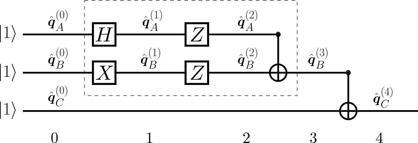
Figure 2: Locality of a quantum circuit of a three-qubit network.

The locality of quantum mechanics is best appreciated in the Heisenberg picture. This is because whereas in the Schrödinger picture quantum information is split between the state vector and the observable, in the Heisenberg picture all dynamical information is carried by a single object: the Heisenberg observable. In this picture, quantum mechanics is not only local but also complete Bedard2021 . This has been known now for more than 20 years Deutsch2000 , and was recently re-explained in Refs. Horsman2007 ; Bedard2021abc ; Bedard2021 ; Kuypers2021 ; RaymondRobichaud2021 . Since our objective is to emphasise the locality of quantum mechanics, we discuss the physics of Fig. 1 in the Heisenberg picture by means of a quantum circuit illustrated in Fig. 2.

The systems $A$, $B$ and $C$ may be regarded as three qubits with Heisenberg observables (or descriptors)

$$\hat{\boldsymbol{q}}_{i}^{(t)}=\left(\hat{q}_{ix}^{(t)},\hat{q}_{iy}^{(t)},\hat{q}_{iz}^{(t)}\right),$$ (10)

with $i=\{A,B,C\}$. The index $i$ implicitly contains the positions of the three qubits $(x_{1},x_{2},x_{3})$. The three-qubit network is initialised with the descriptors

$$\hat{\boldsymbol{q}}_{A}^{(0)} =\left(\hat{\sigma}_{x}\otimes\hat{1}\otimes\hat{1},\hat{\sigma}_{y}\otimes\hat{1}\otimes\hat{1},\hat{\sigma}_{z}\otimes\hat{1}\otimes\hat{1}\right)\equiv(\hat{q}_{Ax},\hat{q}_{Ay},\hat{q}_{Az})\mathchar 24635\relax\;$$

$$\hat{\boldsymbol{q}}_{B}^{(0)} =\left(\hat{1}\otimes\hat{\sigma}_{x}\otimes\hat{1},\hat{1}\otimes\hat{\sigma}_{y}\otimes\hat{1},\hat{1}\otimes\hat{\sigma}_{z}\otimes\hat{1}\right)\equiv(\hat{q}_{Bx},\hat{q}_{By},\hat{q}_{Bz})\mathchar 24635\relax\;$$

$$\hat{\boldsymbol{q}}_{C}^{(0)} =\left(\hat{1}\otimes\hat{1}\otimes\hat{\sigma}_{x},\hat{1}\otimes\hat{1}\otimes\hat{\sigma}_{y},\hat{1}\otimes\hat{1}\otimes\hat{\sigma}_{z}\right)\equiv(\hat{q}_{Cx},\hat{q}_{Cy},\hat{q}_{Cz})\mathchar 24635\relax\;$$ (11)

where $(\hat{\sigma}_{x},\hat{\sigma}_{y},\hat{\sigma}_{z})$ are the Pauli matrices, and $\hat{1}$ is the $2\times 2$ identity matrix; and the fixed Heisenberg state is $|\psi\rangle=-|1\rangle\otimes|1\rangle\otimes|1\rangle$. This state is chosen to reproduce the entangled state Eq. (7) after the evolution of the descriptors, which, in this section’s notation is $|\Psi^{(3)}\rangle=(|1\rangle|-1\rangle-|-1\rangle|1\rangle)/\sqrt{2}$.

In Fig. 2 we show a quantum circuit of a three qubit network that is equivalent to Fig. 1. The dashed box is a type of Bell-gate that entangles the qubits $A$ and $B$ into a singlet configuration, and it serves as a simple model for local interactions. We now evolve the locally specified descriptors according to the protocol in Fig. 2. Below we summarise the effect of the gates of Fig. 2 on the descriptors. The single qubit gates evolve the descriptors as

$$X:\quad\hat{\boldsymbol{q}}_{i}^{(t+1)}=\left(\hat{q}_{ix}^{(t)},-\hat{q}_{iy}^{(t)},-\hat{q}_{iz}^{(t)}\right)\mathchar 24635\relax\;$$

$$Z:\quad\hat{\boldsymbol{q}}_{i}^{(t+1)}=\left(-\hat{q}_{ix}^{(t)},-\hat{q}_{iy}^{(t)},\hat{q}_{iz}^{(t)}\right)\mathchar 24635\relax\;$$

$$H:\quad\hat{\boldsymbol{q}}_{i}^{(t+1)}=\left(\hat{q}_{iz}^{(t)},-\hat{q}_{iy}^{(t)},\hat{q}_{ix}^{(t)}\right).$$ (12)

The controlled not gate $\mathsf{cnot}$ is a simultaneous operation on two neighbouring qubits. One is the control qubit $\mathsf{C}$ and the other the target qubit $\mathsf{T}$. The effect of the $\mathsf{cnot}$ on those qubits is

$$\mathsf{cnot}:\quad\hat{\boldsymbol{q}}_{\mathsf{C}}^{(t+1)} =\left(\hat{q}_{\mathsf{C}x}^{(t)}\hat{q}_{\mathsf{T}x}^{(t)},\hat{q}_{\mathsf{C}y}^{(t)}\hat{q}_{\mathsf{T}x}^{(t)},\hat{q}_{\mathsf{C}z}^{(t)}\right)\mathchar 24635\relax\;$$

$$\hat{\boldsymbol{q}}_{\mathsf{T}}^{(t+1)} =\left(\hat{q}_{\mathsf{T}x}^{(t)},\hat{q}_{\mathsf{T}y}^{(t)}\hat{q}_{\mathsf{C}z}^{(t)},\hat{q}_{\mathsf{T}z}^{(t)}\hat{q}_{\mathsf{C}z}^{(t)}\right).$$ (13)

For the technical details we refer the reader to Refs. Horsman2007 ; Bedard2021abc ; Kuypers2021 .

From $t=0$ to $t=1$, qubit $A$ is subjected to a Hadamard gate $H$ and qubit $B$ to a Pauli-$X$ gate $X$. Using the properties of Eq. (12), we can write the descriptors at $t=1$:

$$\hat{\boldsymbol{q}}_{A}^{(1)} =(\hat{q}_{Az},-\hat{q}_{Ay},\hat{q}_{Ax})\mathchar 24635\relax\;$$

$$\hat{\boldsymbol{q}}_{B}^{(1)} =(\hat{q}_{Bx},-\hat{q}_{By},-\hat{q}_{Bz})\mathchar 24635\relax\;$$

$$\hat{\boldsymbol{q}}_{C}^{(1)} =(\hat{q}_{Cx},\hat{q}_{Cy},\hat{q}_{Cz}).$$ (14)

Because the descriptors are specified locally, one can write the descriptors in Eq. (14) on the circuit legs; see Fig. 2. From $t=1$ to $t=2$, Pauli-$Z$ gates operate on qubits $A$ and $B$, such that at $t=2$, the descriptors evolve to

$$\hat{\boldsymbol{q}}_{A}^{(2)} =(-\hat{q}_{Az},\hat{q}_{Ay},\hat{q}_{Ax})\mathchar 24635\relax\;$$

$$\hat{\boldsymbol{q}}_{B}^{(2)} =(-\hat{q}_{Bx},\hat{q}_{By},-\hat{q}_{Bz})\mathchar 24635\relax\;$$

$$\hat{\boldsymbol{q}}_{C}^{(2)} =(\hat{q}_{Cx},\hat{q}_{Cy},\hat{q}_{Cz}).$$ (15)

In the Heisenberg picture, two qubits $A$ and $B$ are entangled at time $t$ if there is a pair of descriptors such that $\langle\psi|\hat{q}_{A\mu}^{(t)}\hat{q}_{B\nu}^{(t)}|\psi\rangle\neq\langle\psi|\hat{q}_{A\mu}^{(t)}|\psi\rangle\langle\psi|\hat{q}_{B\nu}^{(t)}|\psi\rangle$ Horsman2007 ; Kuypers2021 . With this, one can check that there is no entanglement at $t=2$. Next, a local interaction between qubits $A$ and $B$ is modelled by a $\mathsf{cnot}$ operation on $A$ as the control, and $B$ as the target. This evolves the qubit network to:

$$\hat{\boldsymbol{q}}_{A}^{(3)} =(\hat{q}_{Az}\hat{q}_{Bx},-\hat{q}_{Ay}\hat{q}_{Bx},\hat{q}_{Ax})\mathchar 24635\relax\;$$

$$\hat{\boldsymbol{q}}_{B}^{(3)} =(-\hat{q}_{Bx},\hat{q}_{By}\hat{q}_{Ax},-\hat{q}_{Bz}\hat{q}_{Ax})\mathchar 24635\relax\;$$

$$\hat{\boldsymbol{q}}_{C}^{(3)} =(\hat{q}_{Cx},\hat{q}_{Cy},\hat{q}_{Cz}).$$ (16)

This corresponds to Fig. 1(b). Qubits $A$ and $B$ are now entangled, but unlike in the Schrödinger representation (see Eq. (7)), the descriptors are still locally specified because the positions $(x_{1},x_{2},x_{3})$ are implicitly contained in $(A,B,C)$. Finally, from $t=3$ to $t=4$, qubits $B$ and $C$ interact locally via a $\mathsf{cnot}$ that evolves the descriptors to

$$\hat{\boldsymbol{q}}_{A}^{(4)} =(\hat{q}_{Az}\hat{q}_{Bx},-\hat{q}_{Ay}\hat{q}_{Bx},\hat{q}_{Ax})\mathchar 24635\relax\;$$

$$\hat{\boldsymbol{q}}_{B}^{(4)} =(-\hat{q}_{Bx}\hat{q}_{Cx},\hat{q}_{By}\hat{q}_{Ax}\hat{q}_{Cx},-\hat{q}_{Bz}\hat{q}_{Ax})\mathchar 24635\relax\;$$

$$\hat{\boldsymbol{q}}_{C}^{(4)} =(\hat{q}_{Cx},-\hat{q}_{Cy}\hat{q}_{Bz}\hat{q}_{Ax},-\hat{q}_{Cz}\hat{q}_{Bz}\hat{q}_{Ax}).$$ (17)

This corresponds to the situation in Fig. 1(c), where the three qubits are now entangled. Although qubit $C$ never interacted with $A$, they are now entangled, but not due to a non-local effect. To understand this we must analyse the local information flow of the circuit. When $A$ interacted locally with $B$, $\hat{\boldsymbol{q}}_{B}^{(3)}$ acquired a copy of $A$ in its $y$ and $z$ components. After this, $A$ was sent away so as to never interact again with $B$ or $C$. Next, $B$ moved to the vicinity of $C$ transporting along with it information about $A$. Therefore, when $C$ interacted locally with $B$, not only did $\hat{\boldsymbol{q}}_{C}^{(4)}$ acquire a copy of $B$ in its $y$ and $z$ components, but it also acquired a copy of $A$! Information was transported locally and casually from qubit $A$ to qubit $C$ by qubit $B$.

4 Discussion

4.1 Locality

Superdeterminism, Bohmian mechanics, and Everettian mechanics are not Bell-local, but they all allow for local information flow. Superdeterminism breaks statistical independence, and information is processed locally by the hidden variables, rendering it non-Bell-local. Bohmian mechanics features non-local hidden variables, but the pilot-wave facilitates the local transport of information. Everettian mechanics lacks Bell-locality due to the absence of a preferred foliation, leading to multiple measurement outcomes. However, both superdeterminism and Everettian mechanics qualify as local theories according to the broader sense of locality principles, such as the one mentioned in Sec. 3.1. Similarly, in relational mechanics and Qubism, the significance of measurement outcomes is contingent upon a specific observer’s perspective.

4.2 Ingredients of theories

The most up-to-date no-go theorems do not exclude the possibility of quantum formulations admitting a local information flow. Yet despite alternative options (see Tab. 1), Bell’s 1964 results continue to be advertised for quantum non-locality Brunner2014 , which is a property of collapse/handshake interpretations. In Sec. 2, we showed how current no-go theorems provide us with four viable categories. We have given one example from each of the categories (A), (B) and (D), that allow for a local information flow.

In the $\psi$-ensemble interpretation, information flows locally via the hidden variables. In superdeterminism, the Schrödinger (or Heisenberg) equation is not all there is. The wavefunction is an emergent average description of an yet unresolved additional structure – the hidden variables. They are not required to comply with Bell’s 1964 theorem, because they break the assumption of statistical independence. This comes with correlations that lack in theories admitting statistical independence. Superdeterminism makes peculiar predictions, which might be tested in the future Hossenfelder2011 ; Hossenfelder2014 .

If one dismisses the additional correlations that come with superdeterminism but maintains hidden variables, then Bell’s result enforces a theory with non-local effects, such as Bohmian mechanics. Unlike superdeterminism, where the hidden variables determine the quantum state, in Bohmian mechanics, the wave pilots the particles, which leads to non-local effects on the particles, but not on the waves.

Further, if one gets rid of the Bohmian particles, one is left with the Schrödinger equation only (or the Heisenberg equations of motion). One possible interpretation is Everettian mechanics, where the recording of measurement outcomes on decoherent foliations has no longer precedence over the recording on other foliations. In Fig. 3 we depict how the stripping down of ingredients from the mathematical formalism takes us from correlated hidden variables to the bare foliations.

For the next section, we drop Bohmian mechanics from the discussion, because of its apparent incompatibility with the locality principles from relativity, and the difficulty of formulating guiding equations within the mathematical methods of quantum field theory. Then, for discussion purposes, this leaves us with superdeterministic and Everettian-type quantum theories.

Figure 3: Comparison of the ingredients of the formalisms in the (a) $\psi$-ensemble interpretation, (b) Bohmian mechanics and (c) Everettian mechanics. (a) The cluster of hidden variables $\{\kappa\}_{\uparrow\downarrow}$ is illustrated by the blue and green disks, which determine the state $|\uparrow\downarrow\rangle$. The $\{\kappa\}_{\uparrow\downarrow}$ correlate with the detector settings $(\mathbf{a},\mathbf{b})$, which violates statistical independence. The dotted relative state represents a counterfactual possibility. (b) In Bohmian mechanics, one gains statistical independence. The hidden variables are the particle’s positions $X_{A}(t)$ and $X_{B}(t)$. (c) In Everettian mechanics only the foliations remain.

4.3 Philosophical analysis

One of the reasons behind the proliferation of quantum interpretations is that there is no consensus on the philosophy of science. Contrasting superdeterminism and Everettian mechanics not only allows us to use a test to falsify one of them, but also contrast different philosophies of science. Although both superdeterminism and Everettian mechanics provide a causal, deterministic, and local description of quantum mechanics, both are frequently overlooked.

To avoid subjectivity, let us state two philosophies of science: instrumentalist views usually adopted by advocates of superdeterminism Hossenfelder2020 , and explanatory approaches adopted by Everettians Wallace2012 ; Deutsch2016 . Instrumentalism is motivated by what we observe, and the role of experiments is to increase credence in favour of a particular theory. In this view, better theories are the ones that give better predictions. In contrast, Deutsch’s philosophy of science builds on Popper, and regards fundamental science as explanatory Deutsch2016 ; Deutsch2012 . The purpose of science is then not mapped to a particular prediction, but to conjecture explanations that specify an ontology and how it behaves. Theories that follow this philosophy do not rely on credence. Instead of finding a theory with high credence, scientific methodology finds flaws and deficiencies in a given explanation and seeks to replace it with a better one. There is no guarantee there is something as the truth, let alone a natural evolution towards it through this methodology. However, it does allow us to consistently compare different theories.

Before making the philosophical analysis using Deutsch’s philosophy, we summarise how, within this approach, one of two rival theories might be refuted. Deutsch draws from Popper’s scientific methodology in which a good theory is never confirmed; instead, bad theories are refuted and replaced by better theories. Paraphrasing Ref. Deutsch2016 , a bad theory is one that:

1. does not account for the objects of the explanation; or

2. conflicts with other good theories (theories that observe the opposites of criteria (i) and (iii)); or,

3. is easy to vary.

If a theory displays at least one of the properties above, then it can be made problematic, which then motivates a scientific problem. Therefore, a scientific theory can only be refuted if it has a better rival according to these criteria. If it has no rival, it can at most be made problematic by the same criteria. A crucial scientific test could be an experiment that allows the identification of a better theory.

We now use Deutsch’s philosophy of Ref. Deutsch2016 to contrast superdeterminism with Everettian mechanics, which according to the criteria above, allows for a crucial test to make one of them problematic. For the experimental proposal in Refs. Hossenfelder2011 ; Hossenfelder2014 , one measures the $z$ and $x$ component of a spin observable $\boldsymbol{\sigma}$ alternately. In Everettian mechanics, the outcomes of the alternating measurements are uncorrelated. This is because the eigenstates of $\sigma_{z}$ are not eigenstates of $\sigma_{x}$. In superdeterminism, a sufficiently short time between measurements prevents the hidden variables to change their cluster. Estimates of timescales can be found in Refs. Hossenfelder2011 ; Hossenfelder2014 . Therefore, assuming that such short timescales can be experimentally achieved, superdeterminism predicts the same result between measurements, whereas Everettian mechanics generally predicts different results. If the experiment repeatedly observes the same result, this would be consistent with both superdeterminism and Everettian mechanics. However, superdeterminism would be a better explanation (according to criteria (i)), because it would clarify why only a single result was observed. The explanation is that the hidden variables remained in the same cluster. According to Deutsch’s criteria (i), Everettian mechanics would be refuted, because it could not account for the object of the explanation; in this case, the hidden variables. If only superdeterminism is left as a good unrivalled theory, it cannot be refuted. Superdeterminism could, at most, be made problematic by criteria (i) - (iii). However, if the experiment observes different results, which is the state of the art, then superdeterminism is refuted by criteria (ii) and (iii). The argument can be repeated for other quantum descriptions, such as collapse variants Deutsch2016 .

4.4 Conclusion

Quantum no-go theorems are perhaps the most powerful tools so far to differentiate and test both modifications of quantum mechanics, and quantum mechanics itself. The most famous no-go theorem is Bell’s 1964 inequality, which imposes restrictions on modifications of quantum mechanics. This is understood in the niche community studying the foundations of quantum mechanics but seems to be misunderstood in the larger physics community. We reviewed recent interpretive claims based on Bell’s original inequality. The dominant view seems to conclude from Bell’s theorems that quantum mechanics itself must be non-local. This motivated us to survey recent advances in local quantum theories and present at least two counter-examples with active research programs. Under currently used philosophies of physics, there are at least two quantum descriptions that are local, casual and deterministic. Superdeterminism escapes Bell’s inequality by violating statistical independence. This allows for a hidden variable program that saves the principle of locality, which possibly helps the compatibility with general relativity. However, even unitary quantum mechanics itself admits a mode of description, namely the Heisenberg representation, which is local. A local realist interpretation of the Heisenberg picture is Everettian mechanics.

Acknowledgements

The authors acknowledge professors S. Dahmen, A. Franklin, N. Lima, S. Prado and S. Saunders for discussions concerning issues addressed in this paper. E.N.C. thanks the support of the National Council for Scientific and Technological Development (CNPq), the support of the Coordination of Superior Level Staff Improvement (CAPES) and the support of the British Council through the Women in Science: Gender Equality 2022 Program.

References

- \bibcommenthead
- (1) Bell, J.S.: On the Einstein Podolsky Rosen paradox. Physics Physique Fizika 1, 195–200 (1964). https://doi.org/10.1103/PhysicsPhysiqueFizika.1.195
- (2) Bell, J.S., Aspect, A.: Speakable and Unspeakable in Quantum Mechanics: Collected Papers on Quantum Philosophy, 2nd edn. Cambridge University Press, Cambridge (2004). https://doi.org/10.1017/CBO9780511815676
- (3) Bertlmann, R., Zeilinger, A. (eds.): Quantum [Un]Speakables II. Springer, Switzerland (2017). https://doi.org/10.1007/978-3-319-38987-5
- (4) Maudlin, T.: What Bell did. Journal of Physics A: Mathematical and Theoretical 47(42), 424010 (2014). https://doi.org/10.1088/1751-8113/47/42/424010
- (5) Nurgalieva, N., Renner, R.: Testing quantum theory with thought experiments. Contemporary Physics 61(3), 193–216 (2020). https://doi.org/10.1080/00107514.2021.1880075
- (6) Myrvold, W., Genovese, M., Shimony, A.: Bell’s Theorem. The Stanford Encyclopedia of Philosophy (2021)
- (7) Clauser, J.F., Horne, M.A., Shimony, A., Holt, R.A.: Proposed experiment to test local hidden-variable theories. Phys. Rev. Lett. 23, 880–884 (1969). https://doi.org/10.1103/PhysRevLett.23.880
- (8) Pusey, M.F., Barrett, J., Rudolph, T.: On the reality of the quantum state. Nature Physics 8(6), 475–478 (2012). https://doi.org/10.1038/nphys2309
- (9) Frauchiger, D., Renner, R.: Quantum theory cannot consistently describe the use of itself. Nature Communications 9(1) (2018). https://doi.org/10.1038/s41467-018-05739-8
- (10) Nurgalieva, N., Mathis, S., del Rio, L., Renner, R.: Thought experiments in a quantum computer. arXiv (2022). https://doi.org/10.48550/arxiv.2209.06236
- (11) Schlosshauer, M.A.: Decoherence and the Quantum-To-Classical Transition. Springer, Berlin (2007). https://doi.org/10.1007/978-3-540-35775-9
- (12) Larsson, J.-Å.: Loopholes in Bell Inequality Tests of Local Realism. Journal of Physics A: Mathematical and Theoretical 47(42), 424003 (2014). https://doi.org/10.1088/1751-8113/47/42/424003
- (13) Hance, J.R., Hossenfelder, S.: Bell’s theorem allows local theories of quantum mechanics. Nature Physics (2022). https://doi.org/10.1038/s41567-022-01831-5
- (14) Hossenfelder, S.: Testing Super-Deterministic Hidden Variables Theories. Foundations of Physics 41(9), 1521–1531 (2011). https://doi.org/10.1007/s10701-011-9565-0
- (15) Carroll, S.M., Lodman, J.: Energy Non-conservation in Quantum Mechanics. Foundations of Physics 51(4) (2021). https://doi.org/10.1007/s10701-021-00490-5
- (16) Deutsch, D.: The logic of experimental tests, particularly of Everettian quantum theory. Studies in History and Philosophy of Science Part B: Studies in History and Philosophy of Modern Physics 55, 24–33 (2016). https://doi.org/10.1016/j.shpsb.2016.06.001
- (17) Deutsch, D.: Quantum theory of probability and decisions. Proceedings of the Royal Society of London. Series A: Mathematical, Physical and Engineering Sciences 455(1988), 3129–3137 (1999). https://doi.org/10.1098/rspa.1999.0443
- (18) Zurek, W.H.: Quantum Darwinism. Nature Physics 5(3), 181–188 (2009). https://doi.org/10.1038/nphys1202
- (19) Marletto, C.: Constructor theory of probability. Proceedings of the Royal Society A: Mathematical, Physical and Engineering Sciences 472(2192), 20150883 (2016). https://doi.org/10.1098/rspa.2015.0883
- (20) Sebens, C.T., Carroll, S.M.: Self-locating Uncertainty and the Origin of Probability in Everettian Quantum Mechanics. The British Journal for the Philosophy of Science 69(1), 25–74 (2018). https://doi.org/10.1093/bjps/axw004
- (21) Dürr, D., Lazarovici, D.: Understanding Quantum Mechanics. Springer, Cham (2020). https://doi.org/10.1007/978-3-030-40068-2
- (22) Wharton, K.B., Argaman, N.: Colloquium: Bell’s theorem and locally mediated reformulations of quantum mechanics. Rev. Mod. Phys. 92, 021002 (2020). https://doi.org/10.1103/RevModPhys.92.021002
- (23) Hossenfelder, S., Palmer, T.: Rethinking Superdeterminism. Frontiers in Physics 8 (2020). https://doi.org/10.3389/fphy.2020.00139
- (24) Hossenfelder, S.: Superdeterminism: A Guide for the Perplexed. arXiv (2020). https://doi.org/10.48550/arxiv.2010.01324
- (25) Hance, J.R., Hossenfelder, S.: The wave function as a true ensemble. Proceedings of the Royal Society A: Mathematical, Physical and Engineering Sciences 478(2262), 20210705 (2022). https://doi.org/10.1098/rspa.2021.0705
- (26) Everett, H.: “Relative State” Formulation of Quantum Mechanics. Rev. Mod. Phys. 29, 454–462 (1957). https://doi.org/10.1103/RevModPhys.29.454
- (27) Brown, H.R.: Everettian quantum mechanics. Contemporary Physics 60(4), 299–314 (2019). https://doi.org/10.1080/00107514.2020.1733846
- (28) Kuypers, S., Deutsch, D.: Everettian relative states in the Heisenberg picture. Proceedings of the Royal Society A: Mathematical, Physical and Engineering Sciences 477(2246), 20200783 (2021). https://doi.org/10.1098/rspa.2020.0783
- (29) Rovelli, C.: Relational quantum mechanics. International Journal of Theoretical Physics 35(8), 1637–1678 (1996). https://doi.org/10.1007/bf02302261
- (30) Martin-Dussaud, P., Rovelli, C., Zalamea, F.: The Notion of Locality in Relational Quantum Mechanics. Foundations of Physics 49(2), 96–106 (2019). https://doi.org/%****␣main.bbl␣Line␣450␣****10.1007/s10701-019-00234-6
- (31) Gambini, R., Pullin, J.: The Montevideo Interpretation of Quantum Mechanics: A Short Review. Entropy 20(6), 413 (2018). https://doi.org/10.3390/e20060413
- (32) Fuchs, C.A., Schack, R.: Quantum-Bayesian coherence. Rev. Mod. Phys. 85, 1693–1715 (2013). https://doi.org/10.1103/RevModPhys.85.1693
- (33) Fuchs, C.A., Mermin, N.D., Schack, R.: An introduction to QBism with an application to the locality of quantum mechanics. American Journal of Physics 82(8), 749–754 (2014). https://doi.org/10.1119/1.4874855
- (34) ’t Hooft, G.: The Cellular Automaton Interpretation of Quantum Mechanics. Springer, Cham (2016). https://doi.org/10.1007/978-3-319-41285-6
- (35) Sen, I.: Analysis of the superdeterministic invariant-set theory in a hidden-variable setting. Proceedings of the Royal Society A: Mathematical, Physical and Engineering Sciences 478(2259) (2022). https://doi.org/10.1098/rspa.2021.0667
- (36) Faye, J.: Copenhagen Interpretation of Quantum Mechanics. In: Zalta, E.N. (ed.) The Stanford Encyclopedia of Philosophy, Winter 2019 edn. Metaphysics Research Lab, Stanford University, ??? (2019)
- (37) Ghirardi, G.C., Rimini, A., Weber, T.: Unified dynamics for microscopic and macroscopic systems. Phys. Rev. D 34, 470–491 (1986). https://doi.org/10.1103/PhysRevD.34.470
- (38) Bassi, A., Lochan, K., Satin, S., Singh, T.P., Ulbricht, H.: Models of wave-function collapse, underlying theories, and experimental tests. Rev. Mod. Phys. 85, 471–527 (2013). https://doi.org/10.1103/RevModPhys.85.471
- (39) Cramer, J.G.: The transactional interpretation of quantum mechanics. Rev. Mod. Phys. 58, 647–687 (1986). https://doi.org/10.1103/RevModPhys.58.647
- (40) Kastner, R.E.: The Transactional Interpretation of Quantum Mechanics. Cambridge University Press, Cambridge, England (2017)
- (41) Bohm, D.: A Suggested Interpretation of the Quantum Theory in Terms of “Hidden” Variables. I. Physical Review 85(2), 166–179 (1952). https://doi.org/10.1103/physrev.85.166
- (42) Schlosshauer, M., Kofler, J., Zeilinger, A.: A snapshot of foundational attitudes toward quantum mechanics. Studies in History and Philosophy of Science Part B: Studies in History and Philosophy of Modern Physics 44(3), 222–230 (2013). https://doi.org/10.1016/j.shpsb.2013.04.004
- (43) Sivasundaram, S., Nielsen, K.H.: Surveying the Attitudes of Physicists Concerning Foundational Issues of Quantum Mechanics. arXiv (2016). https://doi.org/10.48550/arxiv.1612.00676
- (44) Gottfried, K., Yan, T.-M.: Quantum Mechanics: Fundamentals, 2nd edn. Graduate Texts in Contemporary Physics. Springer, New York, NY (2004)
- (45) Brunner, N., Cavalcanti, D., Pironio, S., Scarani, V., Wehner, S.: Bell nonlocality. Rev. Mod. Phys. 86, 419–478 (2014). https://doi.org/10.1103/RevModPhys.86.419
- (46) Deutsch, D., Hayden, P.: Information flow in entangled quantum systems. Proceedings of the Royal Society of London. Series A: Mathematical, Physical and Engineering Sciences 456(1999), 1759–1774 (2000). https://doi.org/10.1098/rspa.2000.0585
- (47) Deutsch, D., Marletto, C.: Constructor theory of information. Proceedings of the Royal Society A: Mathematical, Physical and Engineering Sciences 471(2174), 20140540 (2015). https://doi.org/10.1098/rspa.2014.0540
- (48) Raymond-Robichaud, P.: A local-realistic model for quantum theory. Proceedings of the Royal Society A: Mathematical, Physical and Engineering Sciences 477(2250), 20200897 (2021). https://doi.org/10.1098/rspa.2020.0897
- (49) Hossenfelder, S.: Testing superdeterministic conspiracy. Journal of Physics: Conference Series 504, 012018 (2014). https://doi.org/10.1088/1742-6596/504/1/012018
- (50) Rauch, D., Handsteiner, J., Hochrainer, A., Gallicchio, J., Friedman, A.S., Leung, C., Liu, B., Bulla, L., Ecker, S., Steinlechner, F., Ursin, R., Hu, B., Leon, D., Benn, C., Ghedina, A., Cecconi, M., Guth, A.H., Kaiser, D.I., Scheidl, T., Zeilinger, A.: Cosmic Bell Test Using Random Measurement Settings from High-Redshift Quasars. Phys. Rev. Lett. 121, 080403 (2018). https://doi.org/10.1103/PhysRevLett.121.080403
- (51) Maudlin, T.: Philosophy of Physics: Quantum Theory. Princeton Foundations of Contemporary Philosophy. Princeton University Press, Princeton, NJ (2019)
- (52) Dürr, D., Goldstein, S., Norsen, T., Struyve, W., Zanghì, N.: Can Bohmian mechanics be made relativistic? Proc. Math. Phys. Eng. Sci. 470(2162), 20130699 (2014). https://doi.org/10.1098/rspa.2013.0699
- (53) Tipler, F.J.: Quantum nonlocality does not exist. Proceedings of the National Academy of Sciences 111(31), 11281–11286 (2014). https://doi.org/10.1073/pnas.1324238111
- (54) Nielsen, M.A., Chuang, I.L.: Quantum Computation and Quantum Information. Cambridge University Press, Cambridge, England (2010)
- (55) Goldstein, S.: Bohmian Mechanics. The Stanford Encyclopedia of Philosophy (2021)
- (56) Vaidman, L.: Many-Worlds Interpretation of Quantum Mechanics, Fall 2021 edn. Metaphysics Research Lab, Stanford University (2021)
- (57) Wallace, D.: The Emergent Multiverse. Oxford University Press (2012)
- (58) Bédard, C.A.: The cost of quantum locality. Proceedings of the Royal Society A: Mathematical, Physical and Engineering Sciences 477(2246) (2021). https://doi.org/10.1098/rspa.2020.0602
- (59) Deutsch, D.: The Beginning of Infinity. Penguin, New York, NY (2012)
- (60) Deutsch, D.: Quantum theory as a universal physical theory. International Journal of Theoretical Physics 24(1), 1–41 (1985). https://doi.org/10.1007/bf00670071
- (61) Deutsch, D.: Quantum theory, the Church–Turing principle and the universal quantum computer. Proceedings of the Royal Society of London. A. Mathematical and Physical Sciences 400(1818), 97–117 (1985). https://doi.org/10.1098/rspa.1985.0070
- (62) Gerhard, K., Renner, R.: Ambiguity in the branching process of Many-Worlds Theories. In: APS March Meeting Abstracts. APS Meeting Abstracts, vol. 2019, pp. 27–004 (2019)
- (63) Hewitt-Horsman, C., Vedral, V.: Entanglement without nonlocality. Phys. Rev. A 76, 062319 (2007). https://doi.org/10.1103/PhysRevA.76.062319
- (64) Bédard, C.A.: The ABC of Deutsch–Hayden Descriptors. Quantum Reports 3(2), 272–285 (2021). https://doi.org/10.3390/quantum3020017