CoMadOut - A Robust Outlier Detection Algorithm based on CoMAD

Abstract

Unsupervised learning methods are well established in the area of anomaly detection and achieve state of the art performances on outlier data sets. Outliers play a significant role, since they bear the potential to distort the predictions of a machine learning algorithm on a given data set. Especially among PCA-based methods, outliers have an additional destructive potential regarding the result: they may not only distort the orientation and translation of the principal components, they also make it more complicated to detect outliers. To address this problem, we propose the robust outlier detection algorithm CoMadOut, which satisfies two required properties: (1) being robust towards outliers and (2) detecting them. Our outlier detection method using coMAD-PCA defines dependent on its variant an inlier region with a robust noise margin by measures of in-distribution (ID) and out-of-distribution (OOD). These measures allow distribution based outlier scoring for each principal component, and thus, for an appropriate alignment of the decision boundary between normal and abnormal instances. Experiments comparing CoMadOut with traditional, deep and other comparable robust outlier detection methods showed that the performance of the introduced CoMadOut approach is competitive to well established methods related to average precision (AP), recall and area under the receiver operating characteristic (AUROC) curve. In summary our approach can be seen as a robust alternative for outlier detection tasks.

Mathematics Subject Classification]68T99, 68W25, 62H86, 62H25, 62G35

1 Introduction

Anomaly Detection, one of the major fields of unsupervised machine learning, is an integral part of many domains uncovering the deviations of their data generating processes and thus supporting domain experts in their daily work to prevent unwanted scenarios. However, real world data sets are often highly imbalanced due to the rare occurrence of outliers. For predictive methods represent these outliers both obstacle and opportunity at the same time. They can be considered as an obstacle, because they may distort the precision of the machine learning method. On the other hand outliers present an opportunity, since they may reveal irregular or abnormal behaviour and therefore interesting insights. From the aforementioned two aspects, we can derive two properties that an anomaly detection algorithm needs to satisfy, namely (1) to be resilient towards outlying data instances, while at the same time (2) detect them. A preliminary step of many outlier detection approaches is dimensionality reduction. This part is often done by PCAJolliffePCA, a technique exploring the directions of highest variances within the data. This is achieved by computing the eigenvectors of the covariance matrix (directions) and the corresponding eigenvalues (variances). Such eigenpairs allow a transformation from the original data to principal components in lower dimensional subspace, and therewith the task of dimensionality reduction and others. However, the usage of the covariance matrix can make the standard PCA susceptible towards outliers, which has lead to the creation of robust PCA methods, that minimize the influence of such outliers.DBLP:journals/jacm/CandesLMW11 In order to achieve resilience or robustness for PCA-based algorithms, we must ensure that the computed principal components and corresponding eigenvalues are barely, or even better not influenced by instances located out of distribution. In particular this means that robustness is achieved if abnormal instances do not skew the orientation and translation of the eigenvectors and do not lead to an increase or decrease of the eigenvalues.

In this work we introduce CoMadOut, an unsupervised outlier detection method, which shows robustness among other techniques due to outlier resistant CoMAD-PCADBLP:conf/sisap/KazempourH019. While DBLP:conf/sisap/KazempourH019 demonstrate that coMAD (co-median absolute deviation) is potentially robust towards anomalies, it lacks the ability to detect abnormal instances. Therefore, we suggest with this paper a competitive outlier detection approach called CoMadOut which is capable to detect, score and predict outliers.

Since there already exists a plethora of outlier detection methods, we investigate in this work the performance of CoMadOut against a comprehensive selection of state-of-the-art techniques (cf. section LABEL:sect:exp) covering both traditional and Deep Anomaly Detection methods.

In summary, this work provides the following contributions:

1. We introduce the robust outlier detection algorithm CoMadOut (CMO) that derives margin-based decision boundaries by utilizing the noise-resistant eigenpairs of CoMAD-PCA.

2. To align the decision boundaries, we offer several outlier scoring variants of CoMadOut, summerized as CMO*, which simultaneously consider measures of out-of-distribution (tailedness) in order to adapt the CMO baseline approach to different distributions.

3. We detail, how the proposed CMO* variants can be combined to an ensemble approach for outlier detection (CMOEns).

4. We show how CoMAD can be used for robust outlier detection.

5. We conduct extensive experiments comparing and discussing the performance of our methods against competitors and several real-world datasets.

The remaining work is structured as follows. In section 2, we give an overview of related work. Section 3 introduces our CoMadOut ouitlier detection method and elaborate several variants of this method. The experiments are presented in section LABEL:sect:exp, while section LABEL:sect:conclusion concludes the paper.

2 Related Work

In this section, we review the related literature, concerning all approaches intersecting with our approach CoMadOut. Thereby we divide those into three categories: (1) well established traditional outlier detection methods, (2) deep outlier detection methods, and (3) robust estimation and PCA-based methods, where the latter are optimized towards outlier robustness most similar to our proposed method CoMadOut.

2.1 Traditional Methods

The Local Outlier Factor (LOF)LOFbreunigKriegel is a density-based outlier detection method. As such it determines if an object is an outlier based on the $k$NN-neighborhood. Samples which exhibit a significantly lower density in their own local neighborhood compared to the density of other samples and their respective neighborhoods are identified as outliers.

The Isolation Forest (IF)IsoForestLiu method is a tree ensemble approach to identify anomalies. The decision trees of that ensemble are initially constructed by randomly selecting a feature and then performing a random split between its minimum and maximum value recursively. IF is based on the assumption that outliers exhibit a lower occurrence in contrast to ”normal” samples making them appear close to the root of a tree with fewer splits necessary.

The One Class SVM (OCSVM)ocsvmCrammer approach separates all samples from the origin by maximizing the distance from a separating hyperplane to the origin. Therefore, kernels can be utilized to transform the samples into a high dimensional and thus better separable space. Consequently, a binary function computes which regions in the original data space exhibit a high density and are therewith labelled with ”+1” while all other samples (outliers) are labelled with ”-1”.

2.2 Deep Outlier Detection Methods

Two prominent neural network architectures that are commonly used for deep anomaly detection are Vanilla Autoencoders (AE), whose low-dimensional codes compete with those of PCAHinton2006ReducingTD, and Variational Autoencoders (VAE)An2015VariationalAB. The underlying concept for both is fairly similar. An Encoder is trained to embed each training sample, so that it can be projected into a generally lower dimensional latent space and then reconstructed by a Decoder network. The assumption for anomaly detection is now that if a model is trained well on normal data, samples that are abnormal should be hard to reconstruct with the same network and therefore have a high reconstruction error. A threshold is then used to identify these anomalies. Among the different variations of AE, VAEs are special versions of autoencoders. VAEs first encode the input as distributions over the latent space followed by a sampling of samples from the learned distributions. In essence VAEs fit normal distributions on the data and achieve a separation from abnormal samples.

2.3 Robust Estimation and PCA-based Methods

Within this work PCA (Principal Component Analysis) of JolliffePCA is denoted as standard PCA. It is a well-known technique to find patterns in high dimensional data by analysing the variances within the data. As stated in previous chapters, its outlier-sensitive mean of the calculated covariance matrix makes it sensitive towards outliers and thus it is not ideal for subsequent tasks like outlier detection. Thus, a more robust, mean-free version is required to perform reliably on outlier data sets.

CoMAD-PCADBLP:conf/sisap/KazempourH019 follows the same goal as Robust PCA and the core idea behind it is intriguingly simple: Instead of computing the eigendecomposition of the covariance matrix, which is highly susceptible to outliers, the computation is performed on a coMAD matrix Falk1997. Analogously to the covariance matrix, the coMAD matrix represents the median absolute deviation from the median for each dimension and each respective pair of dimensions. Therefore, the coMAD-PCA considers the components with the highest deviation to the median, while standard PCA captures the deviation to the mean. Since the mean of standard PCA is generally more sensitive to outliers OutlierSensitivityOfPCA, coMAD-PCA should be less sensitive. That has been shown by the initial results of DBLP:conf/sisap/KazempourH019, who illustrated the robustness of coMAD-PCA towards outliers.

Amongst the methods that also consider robustness is the so called Minimum Covariance Determinant (MCD)rousseeuw1984least. The goal of MCD is to find a subset of samples whose covariance matrix has the minimum determinant. Its location is then the subset’s average, and its variance is the subset’s covariance matrix. rousseeuw1984least states in addition that this technique can yield suitable results even when 50$\%$ of the data are contaminated with outliers.

Since the performance of Empirical Covariance Estimators, like e.g. the performance of the Maximum Likelihood Covariance Estimator (MLE), suffers from distorted eigenvectors when used on data sets with outliers, more robust methods have been developed. They replace the outlier sensitive parts mean and (co)variance by robust alternatives. These alternatives use e.g. the samples of the lowest covariance matrix determinant (MCD) or randomly selected samples (FastMCD)Rousseeuw98afast to provide a robust mean and covariance or compute it deterministically (DetMCD)Hubert10adeterministic in order to achieve a robust distance measure and thereby a high breakdown value.

By following the goal of getting robust towards outliers there had been several ideas to achieve this. At this point the role of coMAD for CoMadOut (cf. section 3 - step 1) shows parallels to the Stahel–Donoho outlyingness (SDO) measureStahelDonohoOutlyingnessMeasure, which instead uses a weighted mean vector and covariance matrix, and to the comedian approachoutlcomedianapproach, which computes robust mahalanobis distances and weights them by a $\chi^{2}$-distribution-factor to receive a suitable cut-off value instead. Further methods with parallels to the role of coMAD are estimators like LMS (Least Median Squares)rousseeuw1984least which fits to the minimal median squared distances and the estimator MOMAD (Median of Means Absolute Deviation)Depersin2021OnTR, which considers the SDO as notion of depth (close to our notion of robust inlierness in section 3.2) while estimating mean values, which are robust to outliers. PCA-MADHuang2021ARA also address the issue of outlier sensitivity and non-robustness of mean-based PCA by weighting outlier scores based on outlier-sensitive standard PCA projections but MAD-weighted z-score distances instead of outlier resistant and kurtosis-weighted coMAD-PCA projection distances or median based margins as the variants of our approach CoMadOut do (cf. Fig. LABEL:fig:AUROCPCAMAD).

With this brief overview on the literature of state-of-the-art outlier detection methods we differentiated existing methods from our approach. Best to our knowledge there are no other approaches like our CoMadOut baseline (cf. section 3 CMO Steps 1-5) using inlier region enhancing coMAD-based orthogonal distance medians as robustness improving noise margins in combination with coMAD-based robust inlier regions to identify, score and predict outliers. Furthermore, there is no approach like our CoMadOut variants CMO* optimizing coMAD-PCA based outlier scores by simultaneously weighting according to variance or tailedness (cf. section LABEL:sect:CoMadOutStep3CMO* CMO* Steps 1-3).

3 CoMadOut

With this section we introduce CoMadOut (CMO), an unsupervised robust outlier detection algorithm, which follows the assumption that coMAD-based principal components and a robust measure of in-distribution (ID), median $m$, as well as measures of out-of-distribution (OOD), kurtosis $\kappa$, optimize the alignment of the decision boundary between normal and abnormal instances. Thus we introduce besides the baseline algorithm CMO also its variants CMO*. The following paragraphs provide a step-wise explanation and address similarities and differences between the several CMO variants. An overview is provided by the table of Fig. 1.

The common goal of all CoMadOut variants is to first of all obtain outlier resistant subspace orientations. This is achieved by (1) using coMAD-PCADBLP:conf/sisap/KazempourH019 with its robust comedian matrixFalk1997 instead of standard PCA with its outlier sensitive covariance matrix (cf. Fig. 2). This allows CoMadOut to utilize the outlier resistant eigenvectors and eigenvalues of coMAD-PCA in order to receive a robust subspace representation (a coordinate system with axes spanned by the coMAD-PCA eigenvectors) and with that the initial region for inliers for the baseline approach CMO. Since noise is often modeled as a weak form of outliers 10.5555/3086742, CoMadOut improves its outlier robustness and its false positive rate also by (2) an additional noise margin (NM) based on the median of the euclidean orthogonal distances between the samples and their subspace axes $k$ extending the initially computed inlier region.

In particular CoMadOut can be described by the following steps and variants. All variants have step 1 and 2 in common and get variant-specifc from step 3.

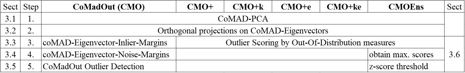
Figure 1: Overview of CoMadOut (CMO) variants and steps.

3.1 Step 1 - Computation of CoMAD-PCA Matrix

Let $X$ be a centered matrix with $n$ samples $x\in\{x_{1},x_{2},...,x_{n}\}$ having $d$-dimensional feature vectors in $\mathbb{R}^{n\times d}$ and let the coMAD matrixFalk1997 be defined by

$$\scriptstyle X=\begin{pmatrix}x_{1,1}&\ldots&x_{1,d}\\ \vdots&\ddots&\vdots\\ x_{n,1}&\ldots&x_{n,d}\\ \end{pmatrix},$$

(1)

with $A_{k}$ being the $k$-th feature of samples $x_{*,k}$ and with

$$comad(A_{i},A_{j})=med((A_{i}-med(A_{i}))(A_{j}-med(A_{j})))$$ (2)

so that the coMAD matrix acts as counterpart for the covariance matrix in the original PCA and

$$A_{i}-med(A_{i})=MAD(A_{i})$$ (3)

represents the robustness providing subtraction of the median in place of the subtraction of the outlier sensitive mean. On the resulting coMAD matrix we apply coMAD-PCADBLP:conf/sisap/KazempourH019 in order to utilize its resulting robust eigenpairs to define the selective inlier region for the CMO baseline. Therefore, we consider

$$coMAD(X)=U\Lambda~{}U^{T}$$ (4)

with eigenvector matrix $U$ and eigenvalue matrix $\Lambda$, where those eigenpairs (consisting out of eigenvector and eigenvalue) with the $k$-largest eigenvalues are used for the definition of the initial inlier region (for CMO baseline) in the next step 2. Since the ideal choice of $K$ for the number of principal components can vary between data sets, we conducted the experiments of our work (cf. section LABEL:sect:exp) on different percentages of the total number of $L$ possible subspaces (leading to a different number of $K$ but maximal $L$ principal components) for all data sets and averaged the achieved average performances.

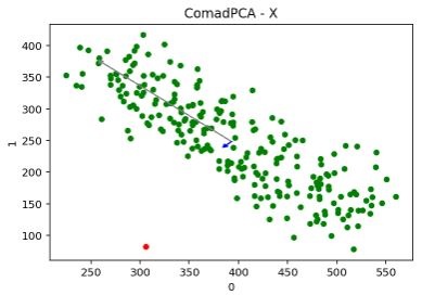
(a) coMAD-PCA

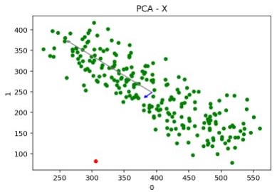
(b) standard PCA

Figure 2: Illustration of orientation and scale of principal components after applying coMAD-PCA (a) and standard PCA (b) to a synthetic data sets. It can be observed that the outlier (colored in red) has less influence to eigenvectors and eigenvalues of coMAD-PCA on the left than to those of standard PCA on the right.

3.2 Step 2 - Orthogonal projections on coMAD-Eigenvectors

In the scope of CoMadOut the previously computed eigenpairs are used to calculate the scores of inlierness and outlierness respectively. Therefore, the orthogonal projections of all samples $x$ are computed for each eigenvector (=principal component). The eigenpairs define the direction ($k$-th eigenvector $\vec{u_{k}}$ of matrix $U$) and scale ($k$-th eigenvalue $\lambda_{k}$ of matrix $\Lambda$) of the corresponding eigenvectors, which correspond to the subspace axes.

Formally step 2 can be described by the following equations: $\forall x\in X$ the projections $x^{\prime}$ can be computed by

$$x^{\prime}=((x^{T}u_{k})/(u_{k}^{T}u_{k}))\cdot u_{k}$$ (5)

Since the origin of the subspace is zero centered after coMAD-PCA from Step 1, the euclidean distances of the projected samples $x^{\prime}$ to the origin can be computed as

$$x’_k = ∑_k=1^K (x_k’)^2 After the first two steps, which have CMO baseline approach and its variants CMO* in common, the next steps are are either related to CMO or to its CMO* variants.  3.3 CMO: Step 3 - Computation of coMAD-Eigenvector-Inlier-Margins The next step for the margin-based CMO baseline approach is to span an initial region for inliers. The eigenpairs define the direction (k-th eigenvector →uk of matrix U) and scale (k-th eigenvalue λk of matrix Λ) of the corresponding eigenvectors, which correspond to the subspace axes. In order to find out which samples x are part of the inlier region, only samples are considered, which got projected on subspace axis k between its origin O and the absolute length of its axis-corresponding eigenvector →uk. Since the eigenvector originally is an unit vector the actual eigenvector length →u_k-andwiththattheinlierrangeforeachsubspaceaxis-isdefinedbythescaleoftherelatedeigenvalueλ_k.Thatλ_kspanstherangeofourinlierregioninpositiveandnegativeeigenvectordirectionwith[-λ_k;+λ_k]oneachsubspaceaxisk.Formally,thedecisionforeachsamplex’,ifitlayswithintheinlierrangeofallsubspaceaxiseigenvectors→u_k,isdefinedasfollows: inl(x′)k={1,ifx'k∈[-λk;+λk]0,otherwiseInordertoavoidinlierstobeconsideredasoutlierswhentheinlierregiondefiningeigenvalueλk (21) =0aminimuminlierregionofϵ=1e-6isdefined.Incaseasamplex'layswithinallinlierrangestheproductofallsubspace-axis-k-relatedinlierfunctionresults inl(x′)=⌈∑k=1Kinl(x′)kK⌉ (8) wouldbeequalto1(=inlier),otherwise0(=non-inlier,cf.sectionLABEL:sect:CoMadOutStep5CMOstep5). 3.4 CMO:Step4 fragmentsx’_k = fragments∑_k=1^K (x_k’)^2 After the first two steps, which have CMO baseline approach and its variants CMO* in common, the next steps are are either related to CMO or to its CMO* variants.  3.3 CMO: Step 3 - Computation of coMAD-Eigenvector-Inlier-Margins The next step for the margin-based CMO baseline approach is to span an initial region for inliers. The eigenpairs define the direction (k-th eigenvector →uk of matrix U) and scale (k-th eigenvalue λk of matrix Λ) of the corresponding eigenvectors, which correspond to the subspace axes. In order to find out which samples x are part of the inlier region, only samples are considered, which got projected on subspace axis k between its origin O and the absolute length of its axis-corresponding eigenvector →uk. Since the eigenvector originally is an unit vector the actual eigenvector length →u_k-andwiththattheinlierrangeforeachsubspaceaxis-isdefinedbythescaleoftherelatedeigenvalueλ_k.Thatλ_kspanstherangeofourinlierregioninpositiveandnegativeeigenvectordirectionwith[-λ_k;+λ_k]oneachsubspaceaxisk.Formally,thedecisionforeachsamplex’,ifitlayswithintheinlierrangeofallsubspaceaxiseigenvectors→u_k,isdefinedasfollows: inl(x′)k={1,ifx'k∈[-λk;+λk]0,otherwiseInordertoavoidinlierstobeconsideredasoutlierswhentheinlierregiondefiningeigenvalueλk (21) =0aminimuminlierregionofϵ=1e-6isdefined.Incaseasamplex'layswithinallinlierrangestheproductofallsubspace-axis-k-relatedinlierfunctionresults inl(x′)=⌈∑k=1Kinl(x′)kK⌉ (8) wouldbeequalto1(=inlier),otherwise0(=non-inlier,cf.sectionLABEL:sect:CoMadOutStep5CMOstep5). 3.4 CMO:Step4 $$ (21)