How do Cross-View and Cross-Modal Alignment
Affect Representations in Contrastive Learning?

Abstract

Various state-of-the-art self-supervised visual representation learning approaches take advantage of data from multiple sensors by aligning the feature representations across views and/or modalities. In this work, we investigate how aligning representations affects the visual features obtained from cross-view and cross-modal contrastive learning on images and point clouds.

On five real-world datasets and on five tasks, we train and evaluate 108 models based on four pretraining variations. We find that cross-modal representation alignment discards complementary visual information, such as color and texture, and instead emphasizes redundant depth cues. The depth cues obtained from pretraining improve downstream depth prediction performance. Also overall, cross-modal alignment leads to more robust encoders than pretraining by cross-view alignment, especially on depth prediction, instance segmentation, and object detection.

1 Introduction

(a)

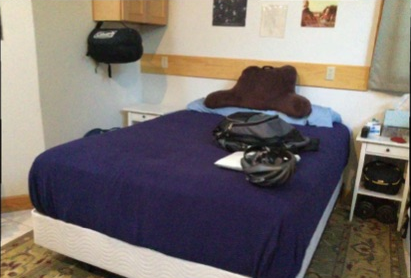
(b)

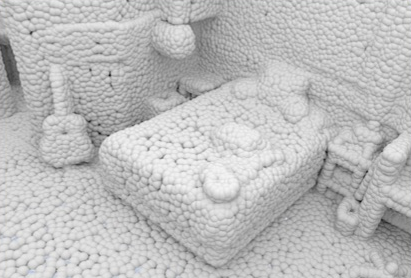
(c)

Figure 1: redundant information is shared across modalities, while complementary information is exclusive to a modality. In this work, we show that cross-modal visual representation learning predominantly encodes redundant information of 2D and 3D data. *Images LABEL:fig:pri3d_rgb and LABEL:fig:pri3d_pc were taken from [1].

Pretraining of neural networks has been an established tool in computer vision for several years [2]. It allows to successfully finetune neural networks on new tasks with fewer iterations and less annotated data [3]. Commonly, models are initialized using weights pretrained for image classification on the ImageNet dataset [4], but recently, self-supervised approaches that do not rely on manual annotations have outperformed ImageNet pretraining [5].

In the realm of self-supervised representation learning, contrastive learning [6] has become a popular approach for visual representation learning. In contrastive learning, the model learns to distinguish different variations of the same instance (e.g. crops of a single image) from all other instances. These variations can be created artificially or by using natural data correspondences, such as images and text [7] or from multiple viewpoints [8, 1].

A common objective is to enforce similarity between features across views or sensing modalities. This is called representation alignment [9]. While severe failure cases of such representation alignment have been discussed [9, 10], the effects on the representation itself were not studied, as of yet.

Figure 1 shows a conceptual illustration of the information available in 2D image data and 3D point clouds in the ScanNet dataset [11]. Some information, such as about depth and surfaces, is available in both modalities. Although this information may be more detailed and more accurate in one modality than in the other, both modalities can express such properties to a certain degree. In the context of sensor fusion, this is typically called redundant information. Other information is exclusive to a modality, which is called complementary information. 3D point clouds, for example, are generally color- and textureless.

Intuitively, a representation which discards complementary information is less expressive than one that includes redundant and complementary information. On the one hand, discarding texture and color information, for example, leads to a less complete visual representation. On the other hand, ImageNet pretrained models were found to be texture-biased and by increasing their shape-bias the performance on tasks such as object detection could be improved [12]. So what is the influence of complementary and redundant information on the visual representation quality?

In this work, we study how complementary and redundant information affect visual representation learning when exploiting cross-view and cross-modal representation alignment, and how this relates to the performance of a finetuned model on a transfer learning downstream task. For this purpose, we use Pri3D [1], a method that uses 3D information of a scene to enable cross-view and cross-modal representation alignment for visual representations learning.

2 Related work

Self-supervised representation learning has recently surpassed supervised pretraining on ImageNet [5]. Various approaches have been explored to learn a global feature vector per image, such as contrastive learning [5, 6] and methods that do not require negative samples during training [13, 14]. Since many computer vision tasks require per-pixel features, several works focused on learning dense representations [15, 16]. Inspired by this success for visual representations, contrastive learning has also been applied to 3D point cloud data [17, 18, 19].

Several approaches have explored cross-modal and cross-view visual representation learning. While some propose a single model [20] for multiple modalities, we are interested in training a vision-only model using cross-modal and cross-view input. To this end, some have matched images and natural language to improve the learned visual representation [7, 21], whereas others use 3D signals [22, 23, 1], or match representations of different views of a scene [8, 1].

While cross-modal feature spaces are a common technique [24, 25, 26, 1, 27, 19], they can introduce several caveats. Especially when dealing with partially incomplete or corrupted data, representation alignment may hinder effective learning for multi-view clustering [9]. In domain adaptation, avoiding representation alignment across modalities has also proven to be beneficial to prevent discarding complementary sensor information [10]. In representation learning, cross-modal training can even lead to an emphasis on a single strong modality and potentially harm the overall performance [28].

Our goal is to understand the effects of cross-view and cross-modal representation alignment on contrastive learning in more detail. Specifically, we do not consider corrupted or incomplete sensor data, but we investigate how redundant and complementary information influence the learned representations, and whether similar effects as observed for shape-biased vs texture-biased networks [12] can be observed. We base our empirical study on Pri3D [1] as it uses both cross-view and cross-modal representation alignment for contrastive learning, as well as their combination. As our main contributions, we:

1. assess how cross-view and cross-modal representation alignment affect the complementary and redundant information encoded in the learned visual per-pixel representations,

2. evaluate the transfer learning performance in different settings on various tasks and datasets to investigate the robustness of cross-view and cross-modal alignment.

3 Methods

2D images and 3D point clouds have low-level redundant and complementary features, as illustrated in Figure 1. Therefore, these modalities lend themselves to study cross-view and cross-modal representation alignment. Our analysis of alignment in representation learning is based on Pri3D [1]. Pri3D uses 3D information for 2D visual representation learning. It employs a self-supervised contrastive learning approach that does not require any human annotation, but only RGB images and registered point clouds that can be obtained, for example, from an RGB-D dataset. This section summarizes the two contrastive losses of Pri3D and discusses how the feature spaces of the losses can be separated.

(a)

(b)

(c)

Figure 2: During pretraining, the combination vgnovVIEWvgnogGEOvgnoddvgnoll (lin)vgnonl (MLP) LABEL:fig:vgno optimizes the same features in the vvVIEWvgGEOvddvll (lin)vnl (MLP) and gvVIEWggGEOgddgll (lin)gnl (MLP) loss, while the linear layer in vgllvVIEWvgllgGEOvgllddvgllll (lin)vgllnl (MLP) LABEL:fig:vgll separates the feature spaces of the losses. The dashed arrows indicate a second overlapping view. Only the 2D backbone performance is evaluated LABEL:fig:downstreamsetup.

3.1 Pri3D: contrastive losses

Pri3D finds pairs of pixels and elements of a regular grid in 3D space, so-called voxels, for contrastive learning. Pixels and voxels are matched by their distance in 3D space to define two losses. One loss requires pairs of pixels across views, whereas the other loss is based on pairs of pixels and 3D points across modalities. Since Pri3D matches pixels and voxels based on their 3D positions, it is relatively robust with respect to incomplete sensor data.

cross-view contrastive loss (vvVIEWvgGEOvddvll (lin)vnl (MLP))

This contrastive loss matches pixels across different views of the same scene. It requires two RGB-D images from the same scene and the corresponding relative camera poses and calibration. Once two pixels from two different views A and B are within a 2 cm distance, they are considered a positive pair in the sense of contrastive learning [6]. Only pixels that are part of a positive pair are used in this loss, as the negative pairs are also constructed from these pixels. To form the negative pairs, each pixel $a$ of view A of a positive pair $(a,b)$ is paired with all pixels $k$ of view B which are part of a positive pair but not $k=b$.

For each image $x$, an encoder-decoder network $f$ predicts a set feature vectors $f(x)$, and $\bm{f}_{a}$ denotes the L2-normalized feature vector of pixel $a$. Using the set of positive pairs $M$, Pri3D employs a PointInfoNCE loss [18]

$$\mathcal{L}_{p}=-\sum_{(a,b)\in M}\log\frac{\exp(\bm{f}_{a}\cdot\bm{f}_{b}/\tau)}{\sum_{(\cdot,k)\in M}\exp(\bm{f}_{a}\cdot\bm{f}_{k}/\tau)},$$ (1)

where $\tau$ is a temperature hyperparameter. This cross-view loss is called the vvVIEWvgGEOvddvll (lin)vnl (MLP) loss, following the convention of Pri3D. Compared to other visual representation learning approaches, vvVIEWvgGEOvddvll (lin)vnl (MLP) does not rely on strong augmentations that may corrupt color information [6].

cross-modal contrastive loss (gvVIEWggGEOgddgll (lin)gnl (MLP))

Unlike the vvVIEWvgGEOvddvll (lin)vnl (MLP) loss, the pairs for the gvVIEWggGEOgddgll (lin)gnl (MLP) loss do not consist of two pixels from different views, but instead of a pixel and a voxel. The positive pairs are again pixels and voxels within 2 cm distance in 3D space. The negative pairs are all other non-matching pixels and voxels pairs, similar to the vvVIEWvgGEOvddvll (lin)vnl (MLP) loss.

The voxel is associated with a feature vector obtained from a dense 3D feature encoder. This dense 3D feature encoder is jointly learned with the dense 2D feature encoder. The loss function (Eq. 1) remains the same with $\bm{f}_{a}$ and $\bm{f}_{b}$ now being feature vectors from the 2D and 3D feature encoders, respectively. Thus, this cross-modal loss enforces the features to be similar across the two modalities and is called the gvVIEWggGEOgddgll (lin)gnl (MLP) loss, following the convention of Pri3D.

3.2 Pri3D: representation space separation

In Pri3D [1], the gvVIEWggGEOgddgll (lin)gnl (MLP) and the vvVIEWvgGEOvddvll (lin)vnl (MLP) loss use the same visual feature vector for a single pixel. Thus, the combination vgvVIEWvggGEOvgddvgll (lin)vgnl (MLP) enforces mutual alignment of cross-view and cross-modal representations. Interestingly, in the implementation published by the original Pri3D authors[29], the feature spaces of both losses are separated by a linear layer preceding the gvVIEWggGEOgddgll (lin)gnl (MLP) loss (see Figure 2). We hypothesize that the original purpose of this layer was merely to match the feature dimensions of the 2D and 3D backbone (e.g. for ResNet50 2D backbone this layer projects 128 to 96 channels). Yet, this separation of feature spaces relaxes the alignment of the cross-view with the cross-modal feature representation. The feature vector of a pixel in the gvVIEWggGEOgddgll (lin)gnl (MLP) loss is now computed by a linear function on the feature vector of the same pixel in the vvVIEWvgGEOvddvll (lin)vnl (MLP) loss, thus the two feature vectors are not the same anymore. The cross-view and the cross-modal representations are not directly aligned. Since the effect of this linear layer was not described in the literature, we include both variants in our experiments.

In the following, we will distinguish this variation by addingllvVIEWllgGEOllddllll (lin)llnl (MLP) to models that include the linear layer that separates the feature representations. These and other differences to the original Pri3D paper are described in more detail in the supplementary material.

4 Experiments

In our experiments, we examine how cross-view and cross-modal representation alignment in Pri3D influence the encoded complementary and redundant information and how possible differences in the representations affect downstream transfer learning performance.

4.1 Setup

The experiments consist of two main steps: We first pretrain models based on the variations of Pri3D (see Section 3). Afterward, the pretrained models are used to initialize training on downstream tasks, where we distinguish between a frozen (Section 4.2), a half-frozen (Section 4.3), and a full finetuning (Section 4.4) setting.

4.1.1 Pretraining

Our implementation is mainly based on the published code of Pri3D, and thus, we follow the same pretraining protocol as presented in the paper [1] and give a coarse outline here. We always use a UNet-style ResNet50 2D backbone and a UNet-style sparse convolutional 3D backbone. As in [1], the 2D backbone is initialized using supervised ImageNet pretraining before performing self-supervised pretraining on the scannetnyuv2NYUv2scannetscannetscannetscannet25kScanNet25kframesScanNetscannetkittiKITTIscannetcityscapesCityscapesscannetcocoCOCO dataset [11]. The scannetnyuv2NYUv2scannetscannetscannetscannet25kScanNet25kframesScanNetscannetkittiKITTIscannetcityscapesCityscapesscannetcocoCOCO dataset is a collection of RGB-D sequences of indoor scenes, captured with a Kinect-like setup. On this dataset, the model is trained for 5 epochs using stochastic gradient descent with a learning rate of 0.1 with polynomial decay of 0.9 and the batch size is 64, unless explicitly mentioned otherwise. This corresponds to approximately 60k iterations and 4 days of training time on 8 Nvidia V100 GPUs for pretraining a single model. The temperature parameter in the losses (Eq. 1) is set to 0.4.

4.1.2 Per-pixel downstream tasks

In Sections 4.2, 4.3 and 4.4 the per-pixel representations are evaluated on depth prediction, image reconstruction, and semantic segmentation while parts of the pretrained network are frozen. To decode the information from features extracted by the frozen pretrained network, we append a non-linear per-pixel MLP (see LABEL:fig:downstreamsetup). This MLP is implemented as a sequence of 1x1 convolutions: Conv1x1@128 $\rightarrow$ ReLU $\rightarrow$ BatchNorm $\rightarrow$ Conv1x1@128 $\rightarrow$ ReLU $\rightarrow$ BatchNorm $\rightarrow$ Conv1x1@$c$ ($c=3$ for image reconstruction, $c=1$ for depth estimation, and $c=\#classes$ for semantic segmentation). The MLP is followed by a bilinear fixed interpolation that upscales the output from $120\times 160$ to $240\times 320$, which is analogous to the semantic segmentation downstream experiments of Pri3D [1] with the UNet architecture. Note that we discard the last convolutional layer from the pretrained model, which, during pretraining, linearly projects the features to the space in which the contrastive loss operates. It can be regarded as the head network which aims to solve the contrastive task.

For image reconstruction and depth prediction, we choose an L2 loss directly on the RGB input pixel values and depth ground truth values, respectively. For semantic segmentation, we use the common cross-entropy loss to predict the semantic classes of each pixel. Other than that, the same training protocol as for the semantic segmentation task in [1] is applied. The mean Intersection-over-Union (mIoU) is the metric for the semantic segmentation quality. The datasets used for depth prediction and image reconstruction are:

• scannet25knyuv2NYUv2scannet25kscannetscannet25kscannet25kScanNet25kframesScanNetscannet25kkittiKITTIscannet25kcityscapesCityscapesscannet25kcocoCOCO [11]: a subset of the scannetnyuv2NYUv2scannetscannetscannetscannet25kScanNet25kframesScanNetscannetkittiKITTIscannetcityscapesCityscapesscannetcocoCOCO dataset annotated for specific tasks, e.g. semantic segmentation, with given training/test/validation splits. The RGB input images of all three splits are subsets of the scannetnyuv2NYUv2scannetscannetscannetscannet25kScanNet25kframesScanNetscannetkittiKITTIscannetcityscapesCityscapesscannetcocoCOCO dataset used for pretraining. On all downstream tasks, we always use scannet25knyuv2NYUv2scannet25kscannetscannet25kscannet25kScanNet25kframesScanNetscannet25kkittiKITTIscannet25kcityscapesCityscapesscannet25kcocoCOCO and therefore do not distinguish it from scannetnyuv2NYUv2scannetscannetscannetscannet25kScanNet25kframesScanNetscannetkittiKITTIscannetcityscapesCityscapesscannetcocoCOCO explicitly.

• nyuv2nyuv2NYUv2nyuv2scannetnyuv2scannet25kScanNet25kframesScanNetnyuv2kittiKITTInyuv2cityscapesCityscapesnyuv2cocoCOCO [30]: A dataset of 1449 RGBD images with semantic segmentation annotations, capturing 464 indoor scenes.

For semantic segmentation, we additionally use the following datasets:

• kittinyuv2NYUv2kittiscannetkittiscannet25kScanNet25kframesScanNetkittikittiKITTIkitticityscapesCityscapeskitticocoCOCO [31]: The dataset of the KITTI semantic segmentation benchmark consists of 200 semantically annotated training as well as 200 test images (our validation set) of road traffic scenes.

• cityscapesnyuv2NYUv2cityscapesscannetcityscapesscannet25kScanNet25kframesScanNetcityscapeskittiKITTIcityscapescityscapesCityscapescityscapescocoCOCO [32]: A dataset of 5000 semantically annotated frames of urban street scenes in 50 different cities.

4.1.3 Object-centered downstream tasks

To perform object detection and instance segmentation, the encoders of the pretrained models are used to initialize a Mask RCNN model [33] of the Detectron2 library [34] in Section 4.5. Due to the downstream architecture, the decoders are discarded. In addition to scannet25knyuv2NYUv2scannet25kscannetscannet25kscannet25kScanNet25kframesScanNetscannet25kkittiKITTIscannet25kcityscapesCityscapesscannet25kcocoCOCO and nyuv2nyuv2NYUv2nyuv2scannetnyuv2scannet25kScanNet25kframesScanNetnyuv2kittiKITTInyuv2cityscapesCityscapesnyuv2cocoCOCO, the models are evaluated on the 2017 version of the coconyuv2NYUv2cocoscannetcocoscannet25kScanNet25kframesScanNetcocokittiKITTIcococityscapesCityscapescocococoCOCO dataset [35] that contains more than 118k training and 5000 validation images. The Average Precision (AP) metric is used on all datasets.

Table 1: Validation performance on the three tasks and four datasets. Rows 1-4 show the frozen downstream setting where the pretrained weights are fixed, in rows 5-8 the encoder of the UNet-style architecture is fixed, and in the last four rows, the entire models are finetuned. To have a consistent notion that a greater value means better performance, the negative L2-Loss is shown. Blue color indicates relative improvement with respect to the cross-view model (vvVIEWvgGEOvddvll (lin)vnl (MLP)).

4.2 Frozen downstream tasks

With the frozen downstream tasks, where we keep all weights of the pretrained network frozen, we investigate how well the pretrained models capture color, depth, or semantic information by predicting this information from the learned per-pixel representations. Using these frozen downstream tasks, we show how the different alignment strategies in Pri3D influence the learned representations. For semantic segmentation, this frozen setup is similar to the linear evaluation protocol commonly used to evaluate the quality of global image features in visual representation learning [6]. In this linear evaluation protocol, the performance of a linear classifier on the global features is often regarded as a proxy metric for the representation quality. In our setup, we evaluate whether a non-linear MLP can provide a proxy metric for the representation quality.

Figure 3: Image reconstructions obtained from different frozen representations. The rows correspond to different samples. The rightmost column is the ground truth data and also the input for the feature extractors. The other columns use different models to compute the features from which the images are reconstructed.

Figure 4: Qualitative results on the frozen depth prediction task. Each row corresponds to one sample and the rightmost column shows the ground truth depth data (saturated blue indicates invalid values). The other columns use different models to compute the frozen per-pixel features for depth prediction.

The first four rows of Table 1 show the best performance on the validation data during the training process for each model variation and frozen downstream task. Compared to the cross-view model (vvVIEWvgGEOvddvll (lin)vnl (MLP)), all other models perform worse on frozen image reconstruction and semantic segmentation. In contrast, the models that include the cross-modal gvVIEWggGEOgddgll (lin)gnl (MLP) loss perform better than the vvVIEWvgGEOvddvll (lin)vnl (MLP) on ScanNet depth prediction, while on NYUv2 this general trend is not visible. The vgllvVIEWvgllgGEOvgllddvgllll (lin)vgllnl (MLP) model outperforms the vgnovVIEWvgnogGEOvgnoddvgnoll (lin)vgnonl (MLP) model on all three frozen downstream tasks by more than 10%.

Figures 3 and 4 show the qualitative reconstruction and depth prediction results. In both cases, the ranking of the models on ScanNet is reflected in the visual reconstruction quality. The vvVIEWvgGEOvddvll (lin)vnl (MLP) model achieves the best visual reconstruction, followed by the vgllvVIEWvgllgGEOvgllddvgllll (lin)vgllnl (MLP), vgnovVIEWvgnogGEOvgnoddvgnoll (lin)vgnonl (MLP) and gvVIEWggGEOgddgll (lin)gnl (MLP) models. It is notable that the results differ especially on flat texture-rich surfaces, for example in the first row where the gvVIEWggGEOgddgll (lin)gnl (MLP) model does recover the wallpaper. All model variations discard most of the color information. The most detailed and smoothest depth estimation is obtained by the vgllvVIEWvgllgGEOvgllddvgllll (lin)vgllnl (MLP) model. The depth gradient along surfaces appears smooth whereas the depth estimation based on vgnovVIEWvgnogGEOvgnoddvgnoll (lin)vgnonl (MLP) and vvVIEWvgGEOvddvll (lin)vnl (MLP) is speckled on flat surfaces.

In conclusion, the cross-view vvVIEWvgGEOvddvll (lin)vnl (MLP) loss preserves more texture information while the cross-modal gvVIEWggGEOgddgll (lin)gnl (MLP) loss leads to a better depth representation. This observation is in line with the ideas of complementary and redundant information discussed in Figure 1. Interestingly, combining the two losses as vgnovVIEWvgnogGEOvgnoddvgnoll (lin)vgnonl (MLP) and aligning the representations across views and modalities only achieves mediocre performance on all three downstream tasks. Once alignment is lifted by the linear layer in vgllvVIEWvgllgGEOvgllddvgllll (lin)vgllnl (MLP), all metrics improve, showing that it allows the model to preserve more complementary information. Notably, the depth prediction result is even better than for the gvVIEWggGEOgddgll (lin)gnl (MLP) model, suggesting that even with respect to the redundant information, this separation is beneficial. The semantic segmentation performance differs strongly between the model variations and benefits from the cross-view loss and the linear layer in vgllvVIEWvgllgGEOvgllddvgllll (lin)vgllnl (MLP) that lifts the direct alignment.

4.3 Half-frozen downstream tasks

By freezing only the encoder part of the UNet-style models, the following experiments provide insight to which part of architecture discards the texture information. The experimental setup, architecture, and datasets remain the same as for the frozen downstream tasks in Section 4.2, except that now also the decoder is finetuned together with the MLP and only the encoder is fixed during finetuning.

The gvVIEWggGEOgddgll (lin)gnl (MLP) model performs best across all tasks and datasets as seen in rows 5-8 of Table 1. The model excels on depth prediction, and interestingly, also outperforms the vvVIEWvgGEOvddvll (lin)vnl (MLP) model on image reconstruction. The combined models outperform vvVIEWvgGEOvddvll (lin)vnl (MLP) on depth prediction, but the other tasks show mixed results. The linear layerllvVIEWllgGEOllddllll (lin)llnl (MLP) improves the vgvVIEWvggGEOvgddvgll (lin)vgnl (MLP) performance slightly.

Overall, the results are in stark contrast to the frozen downstream tasks. Given that the gvVIEWggGEOgddgll (lin)gnl (MLP) model outperforms the vvVIEWvgGEOvddvll (lin)vnl (MLP) model, it seems that the decoder discards the texture information in the frozen downstream tasks, and recovering the texture is possible by finetuning. At the same time, the encoder of the gvVIEWggGEOgddgll (lin)gnl (MLP) model extracts very robust features across tasks and datasets.

4.4 Full finetuning downstream tasks

To assess the practical value and generality of a visual representation, the models are now fully finetuned and evaluated on the downstream tasks. In contrast to the frozen downstream tasks, all weights in the model are finetuned during the downstream task training. As the full model is finetuned, the per-pixel MLP is not needed anymore and is omitted.

Rows 9-12 in Table 1 show the full finetuning downstream performance. Models that were trained including the gvVIEWggGEOgddgll (lin)gnl (MLP) loss outperform the vvVIEWvgGEOvddvll (lin)vnl (MLP) model on depth prediction. Again, gvVIEWggGEOgddgll (lin)gnl (MLP) is the best model for image reconstruction. On semantic segmentation, vvVIEWvgGEOvddvll (lin)vnl (MLP) performs best on cityscapesnyuv2NYUv2cityscapesscannetcityscapesscannet25kScanNet25kframesScanNetcityscapeskittiKITTIcityscapescityscapesCityscapescityscapescocoCOCO and kittinyuv2NYUv2kittiscannetkittiscannet25kScanNet25kframesScanNetkittikittiKITTIkitticityscapesCityscapeskitticocoCOCO, but not on the other two datasets.

Also in this full finetuning setting, cross-modal alignment improves depth prediction performance. For semantic segmentation, the results are generally mixed, but it is notable that vvVIEWvgGEOvddvll (lin)vnl (MLP) performs well on the two outdoor datasets. This may indicate that the cross-modal models are biased towards spatial layouts of indoor scenes. Adding the feature space separationllvVIEWllgGEOllddllll (lin)llnl (MLP) to vgvVIEWvggGEOvgddvgll (lin)vgnl (MLP) does not have a positive effect, but rather tends to decrease the performance.

4.5 Instance and object segmentation

As discussed in [12], texture-biased networks are inferior to shape-biased networks for object detection. In order to test whether this also holds for texture-biased networks compared to depth-biased networks, the pretrained encoders are finetuned for object detection and instance segmentation.

Table 2: Comparison of instance segmentation and object detection performance of the four different models (rows). Blue color indicates relative improvement with respect to the cross-view model (vvVIEWvgGEOvddvll (lin)vnl (MLP)).

Table 2 shows that the cross-modal gvVIEWggGEOgddgll (lin)gnl (MLP) model outperforms the vvVIEWvgGEOvddvll (lin)vnl (MLP) model on 5 out of 6 task and dataset combinations. The combined models vgnovVIEWvgnogGEOvgnoddvgnoll (lin)vgnonl (MLP) and vgllvVIEWvgllgGEOvgllddvgllll (lin)vgllnl (MLP) models show mixed results, perform well on scannetnyuv2NYUv2scannetscannetscannetscannet25kScanNet25kframesScanNetscannetkittiKITTIscannetcityscapesCityscapesscannetcocoCOCO, but not on coconyuv2NYUv2cocoscannetcocoscannet25kScanNet25kframesScanNetcocokittiKITTIcococityscapesCityscapescocococoCOCO. On nyuv2nyuv2NYUv2nyuv2scannetnyuv2scannet25kScanNet25kframesScanNetnyuv2kittiKITTInyuv2cityscapesCityscapesnyuv2cocoCOCO, their difference is most pronounced where the linear feature separationllvVIEWllgGEOllddllll (lin)llnl (MLP) leads to the worst performance among the four model variations while omitting it results in the best performance.

Combining the losses in the vgnovVIEWvgnogGEOvgnoddvgnoll (lin)vgnonl (MLP) and vgllvVIEWvgllgGEOvgllddvgllll (lin)vgllnl (MLP) models seems to be beneficial within the pretraining dataset, but not when shifting domains. Overall, although the performance differences are small, the gvVIEWggGEOgddgll (lin)gnl (MLP) model appears to be more robust. This supports the idea that texture-biased networks are not as robust for object-centered tasks as the depth-biased gvVIEWggGEOgddgll (lin)gnl (MLP) network.

5 Discussion

The comparison on the frozen downstream tasks reveals that cross-view and cross-modal representation alignment influence the complementary and redundant information encoded in the learned representations. While the vvVIEWvgGEOvddvll (lin)vnl (MLP) model preserves the texture and the gvVIEWggGEOgddgll (lin)gnl (MLP) model preserves the depth, the combination vgnovVIEWvgnogGEOvgnoddvgnoll (lin)vgnonl (MLP) does not result in the different low-level features complementing each other, but instead a fully shared feature space is obtained where complementary information is lost and redundant details are less accentuated. vgllvVIEWvgllgGEOvgllddvgllll (lin)vgllnl (MLP) improves the combined model on all three frozen downstream tasks and raises the question of whether this means we have found a generally better representation. The performance on the half-frozen and full finetuning downstream tasks contradict this apparent conclusion and we even find that the gvVIEWggGEOgddgll (lin)gnl (MLP) model performs most robustly across tasks and datasets. This shows that reducing texture-bias in networks increases robustness, similar to findings in [12].

On semantic segmentation, the frozen downstream task shows a distinct ranking that is persistent across datasets. These distinct performance differences were not observed once the decoder is finetuned as well. A possible explanation could be that the texture-bias is to a certain degree useful but also easy to recover and thus not important to learn during pretraining. So although the strong differences on the frozen downstream tasks reveal that the diverse representations either incorporate or discard complementary information, the performance on the frozen tasks does not correlate with the finetuning downstream performance.

The comparison of vgnovVIEWvgnogGEOvgnoddvgnoll (lin)vgnonl (MLP) with vvVIEWvgGEOvddvll (lin)vnl (MLP) and gvVIEWggGEOgddgll (lin)gnl (MLP) indicates different behavior on data within the same domain and across domains. The vgnovVIEWvgnogGEOvgnoddvgnoll (lin)vgnonl (MLP) model excels especially in object detection, instance segmentation, and semantic segmentation on the scannetnyuv2NYUv2scannetscannetscannetscannet25kScanNet25kframesScanNetscannetkittiKITTIscannetcityscapesCityscapesscannetcocoCOCO dataset. A similar effect of overfitting to the pretraining dataset is also reflected in the learning rate variations shown in the supplementary material. In a broader context, this could mean that aligning cross-modal and cross-view representations may harm generalization across datasets but could prove especially useful when exploiting unlabelled data within the same domain for better performance on a small annotated subset. Still, further experiments are needed to verify this hypothesis.

Our empirical study comes with certain limitations. Although our results are obtained on various datasets and tasks, the pretraining and finetuning results are always subject to stochastic effects in the training processes. Further, we only focused on the most obvious modality-specific information such as color and depth. The image reconstruction and depth prediction tasks only test some characteristics of the learned representations while other characteristics may be more indicative with respect to downstream finetuning performance. Still, our results show that the different pretraining strategies yield representations that encode different information.

6 Conclusions and future work

Aligning feature representations across views and across modalities is a common approach in self-supervised learning. Yet, the effects on the learned visual representations are often not well understood. We showed quantitatively that, in contrast to cross-view representation alignment, cross-modal representation alignment can lead to discarding complementary information of the individual modalities. In the context of cross-modal learning on images and point clouds, texture is considered complementary information of the visual data and depth is redundant information. Pretraining by cross-modal alignment was especially useful for tasks that require a notion of the spatial layout, such as depth prediction, and also instance segmentation and object detection. This effect is similar to the observations of previous work that shape-biased networks are more robust than texture-biased networks. Thus, pretraining with emphasis on the redundant information achieved the most robust performance when finetuning the visual backbone networks on various downstream tasks and datasets.

Merging complementary information is a fundamental goal of sensor fusion and discarding that information may harm the overall performance on such a task. While our results have indicated that visual representations become more robust by reducing the texture-bias through cross-modal alignment, future work should investigate whether these results still hold for self-supervised approaches that fuse different sensing modalities.

References

- [1] Ji Hou, Saining Xie, Benjamin Graham, Angela Dai, and Matthias Nießner. Pri3d: Can 3d priors help 2d representation learning? In Proc. of the IEEE/CVF International Conference on Computer Vision, pages 5693–5702, 2021.
- [2] Matthew D Zeiler and Rob Fergus. Visualizing and understanding convolutional networks. In European Conference on Computer Vision, pages 818–833. Springer, 2014.
- [3] Kaiming He, Ross Girshick, and Piotr Dollár. Rethinking ImageNet pre-training. In Proc. of the IEEE/CVF International Conference on Computer Vision, pages 4918–4927, 2019.
- [4] Olga Russakovsky, Jia Deng, Hao Su, Jonathan Krause, Sanjeev Satheesh, Sean Ma, Zhiheng Huang, Andrej Karpathy, Aditya Khosla, Michael Bernstein, Alexander C. Berg, and Li Fei-Fei. ImageNet Large Scale Visual Recognition Challenge. International Journal of Computer Vision, 115(3):211–252, 2015.
- [5] Kaiming He, Haoqi Fan, Yuxin Wu, Saining Xie, and Ross Girshick. Momentum contrast for unsupervised visual representation learning. In Proc. of the IEEE Conference on Computer Vision and Pattern Recognition, pages 9729–9738, 2020.
- [6] Ting Chen, Simon Kornblith, Mohammad Norouzi, and Geoffrey Hinton. A simple framework for contrastive learning of visual representations. In International conference on machine learning, pages 1597–1607. PMLR, 2020.
- [7] Xin Yuan, Zhe Lin, Jason Kuen, Jianming Zhang, Yilin Wang, Michael Maire, Ajinkya Kale, and Baldo Faieta. Multimodal Contrastive Training for Visual Representation Learning. In Proc. of the IEEE Conference on Computer Vision and Pattern Recognition, pages 6995–7004, 2021.
- [8] Yonglong Tian, Dilip Krishnan, and Phillip Isola. Contrastive multiview coding. In European Conference on Computer Vision, pages 776–794. Springer, 2020.
- [9] Daniel Trosten, Sigurd Lokse, Robert Jenssen, and Michael Kampffmeyer. Reconsidering Representation Alignment for Multi-view Clustering. In Proc. of the IEEE Conference on Computer Vision and Pattern Recognition, pages 1255–1265, 2021.
- [10] Maximilian Jaritz, Tuan-Hung Vu, Raoul de Charette, Emilie Wirbel, and Patrick Pérez. xMUDA: Cross-modal unsupervised domain adaptation for 3d semantic segmentation. In Proc. of the IEEE Conference on Computer Vision and Pattern Recognition, pages 12605–12614, 2020.
- [11] Angela Dai, Angel X Chang, Manolis Savva, Maciej Halber, Thomas Funkhouser, and Matthias Nießner. ScanNet: Richly-annotated 3d reconstructions of indoor scenes. In Proc. of the IEEE Conference on Computer Vision and Pattern Recognition, pages 5828–5839, 2017.
- [12] R. Geirhos, P. Rubisch, C. Michaelis, M. Bethge, F. A. Wichmann, and W. Brendel. ImageNet-trained CNNs are biased towards texture; increasing shape bias improves accuracy and robustness. In International Conference on Learning Representations, May 2019.
- [13] Xinlei Chen and Kaiming He. Exploring simple siamese representation learning. In Proc. of the IEEE Conference on Computer Vision and Pattern Recognition, pages 15750–15758, 2021.
- [14] Jean-Bastien Grill, Florian Strub, Florent Altché, Corentin Tallec, Pierre Richemond, Elena Buchatskaya, Carl Doersch, Bernardo Avila Pires, Zhaohan Guo, Mohammad Gheshlaghi Azar, Bilal Piot, Koray Kavukcuoglu, Remi Munos, and Michal Valko. Bootstrap your own latent-a new approach to self-supervised learning. Advances in Neural Information Processing Systems, 33:21271–21284, 2020.
- [15] Xinlong Wang, Rufeng Zhang, Chunhua Shen, Tao Kong, and Lei Li. Dense Contrastive Learning for Self-Supervised Visual Pre-Training. In Proc. of the IEEE Conference on Computer Vision and Pattern Recognition, 2021.
- [16] Zhenda Xie, Yutong Lin, Zheng Zhang, Yue Cao, Stephen Lin, and Han Hu. Propagate Yourself: Exploring Pixel-Level Consistency for Unsupervised Visual Representation Learning. In Proc. of the IEEE Conference on Computer Vision and Pattern Recognition, pages 16684–16693, June 2021.
- [17] Ji Hou, Benjamin Graham, Matthias Nießner, and Saining Xie. Exploring data-efficient 3d scene understanding with contrastive scene contexts. In Proc. of the IEEE Conference on Computer Vision and Pattern Recognition, pages 15587–15597, 2021.
- [18] Saining Xie, Jiatao Gu, Demi Guo, Charles R Qi, Leonidas Guibas, and Or Litany. PointContrast: Unsupervised pre-training for 3d point cloud understanding. In European Conference on Computer Vision, pages 574–591. Springer, 2020.
- [19] Zaiwei Zhang, Rohit Girdhar, Armand Joulin, and Ishan Misra. Self-supervised pretraining of 3d features on any point-cloud. arXiv preprint arXiv:2101.02691, 2021.
- [20] Yunze Liu, Qingnan Fan, Shanghang Zhang, Hao Dong, Thomas Funkhouser, and Li Yi. Contrastive multimodal fusion with TupleInfoNCE. In Proc. of the IEEE/CVF International Conference on Computer Vision, pages 754–763, 2021.
- [21] Alec Radford, Jong Wook Kim, Chris Hallacy, Aditya Ramesh, Gabriel Goh, Sandhini Agarwal, Girish Sastry, Amanda Askell, Pamela Mishkin, Jack Clark, et al. Learning transferable visual models from natural language supervision. arXiv preprint arXiv:2103.00020, 2021.
- [22] Zhenyu Li, Zehui Chen, Ang Li, Liangji Fang, Qinhong Jiang, Xianming Liu, Junjun Jiang, Bolei Zhou, and Hang Zhao. SimIPU: Simple 2D Image and 3D Point Cloud Unsupervised Pre-Training for Spatial-Aware Visual Representations. arXiv preprint arXiv:2112.04680, 2022.
- [23] Longlong Jing, Ling Zhang, and Yingli Tian. Self-supervised feature learning by cross-modality and cross-view correspondences. In IEEE/CVF Conference on Computer Vision and Pattern Recognition Workshops, pages 1581–1891. IEEE, 2021.
- [24] Nawid Sayed, Biagio Brattoli, and Björn Ommer. Cross and learn: Cross-modal self-supervision. In German Conference on Pattern Recognition, pages 228–243. Springer, 2018.
- [25] Saurabh Gupta, Judy Hoffman, and Jitendra Malik. Cross modal distillation for supervision transfer. In Proc. of the IEEE Conference on Computer Vision and Pattern Recognition, pages 2827–2836, 2016.
- [26] Adrian Benton, Huda Khayrallah, Biman Gujral, Dee Ann Reisinger, Sheng Zhang, and Raman Arora. Deep generalized canonical correlation analysis. arXiv preprint arXiv:1702.02519, 2017.
- [27] Michelle A. Lee, Matthew Tan, Yuke Zhu, and Jeannette Bohg. Detect, Reject, Correct: Crossmodal Compensation of Corrupted Sensors. In Proc. of the IEEE International Conference on Robotics and Automation, Xi’an, China, 2021.
- [28] Yunze Liu, Li Yi, Shanghang Zhang, Qingnan Fan, Thomas Funkhouser, and Hao Dong. P4Contrast: Contrastive Learning with Pairs of Point-Pixel Pairs for RGB-D Scene Understanding. arXiv preprint arXiv:2012.13089, 2020.
- [29] Ji Hou. Pri3d. https://github.com/Sekunde/Pri3D (commit 9086edd), 2021.
- [30] Nathan Silberman, Derek Hoiem, Pushmeet Kohli, and Rob Fergus. Indoor segmentation and support inference from RGBD images. In European Conference on Computer Vision, pages 746–760. Springer, 2012.
- [31] Hassan Alhaija, Siva Mustikovela, Lars Mescheder, Andreas Geiger, and Carsten Rother. Augmented Reality Meets Computer Vision: Efficient Data Generation for Urban Driving Scenes. International Journal of Computer Vision, 2018.
- [32] Marius Cordts, Mohamed Omran, Sebastian Ramos, Timo Rehfeld, Markus Enzweiler, Rodrigo Benenson, Uwe Franke, Stefan Roth, and Bernt Schiele. The Cityscapes Dataset for Semantic Urban Scene Understanding. In Proc. of the IEEE Conference on Computer Vision and Pattern Recognition, 2016.
- [33] Kaiming He, Georgia Gkioxari, Piotr Dollár, and Ross Girshick. Mask R-CNN. In Proc. of the IEEE/CVF International Conference on Computer Vision, pages 2961–2969, 2017.
- [34] Yuxin Wu, Alexander Kirillov, Francisco Massa, Wan-Yen Lo, and Ross Girshick. Detectron2. https://github.com/facebookresearch/detectron2, 2019.
- [35] Tsung-Yi Lin, Michael Maire, Serge Belongie, James Hays, Pietro Perona, Deva Ramanan, Piotr Dollár, and C Lawrence Zitnick. Microsoft COCO: Common objects in context. In European Conference on Computer Vision, pages 740–755. Springer, 2014.