Shapley Curves: A Smoothing Perspective

Abstract

Originating from cooperative game theory, Shapley values have become one of the most widely used measures for variable importance in applied Machine Learning. However, the statistical understanding of Shapley values is still limited. In this paper, we take a nonparametric (or smoothing) perspective by introducing Shapley curves as a local measure of variable importance. We consider two estimation strategies and derive the consistency and asymptotic normality both under independence and dependence among the features. We further propose a novel version of the wild bootstrap procedure specifically adjusted for Shapley curves. This allows us to construct confidence intervals and conduct inference. The asymptotic results are validated in extensive experiments. In an empirical application, we analyze which attributes drive the prices of vehicles.

Keywords: Variable importance, nonparametric statistics, explainable ML, additive models

1 Introduction

Modern data science techniques like deep neural networks and ensemble methods such as gradient boosting are well-known for yielding high prediction accuracy. However, it is barely understood how the output depends on the input variables for these techniques. Consequently, the lack of transparency within these black boxes is limiting the practical use of machine learning (ML), since decision-makers require profound reasoning for critical applications such as medical diagnoses, credit scoring or price setting. One way of navigating this issue is to estimate the importance of the variables at hand.

A variable importance measure that recently has gained in popularity is the Shapley value. Shapley values enable the statistician to explain predictions on a local level, where each variable is assigned an importance measure in explaining the dependent variable for a particular observation. The idea of Shapley values originates from game theory and was proposed for giving a unique solution to a cooperative game (Shapley, 1953). Hereby, the goal is to assign credit to each player, according to their contribution to a total payoff in the cooperative game. An analogy is found in statistics, where the interest is in assigning an importance measure for each variable. For example, Lundberg and Lee (2017) define the Shapley values to explain predictions of the conditional mean. Other works make use of this flexibility by defining their version in terms of predictiveness measures such as the variance of the conditional mean (Bénard et al., 2022a; Owen and Prieur, 2017) or even $R^{2}$ and mean-squared-error (Williamson and Feng, 2020).

Previous literature is mainly concerned with the practical computation of Shapley values, particularly focusing on computational efficiency (Bénard et al., 2022a; Lundberg et al., 2020). To the best of our knowledge, barely any paper approached the topic from a nonparametric perspective, in which it is possible to deduce precise asymptotic results for variable importance measures. We are aware that an asymptotic result is not in the immediate interest of a “high prediction accuracy” data scientist. However, we seek to fill this gap of asymptotics in the interest of explainable ML by considering $d$-dimensional Shapley curves instead of point-wise Shapley values, thereby convergence of the whole curve is established. In contrast to the previous literature, the Shapley curves result in a variable importance measure for any arbitrary evaluation point in the $d$-dimensional input space.

In order to establish asymptotic results we a priori define the Shapley curves on population level. It is uniquely determined by the $d$-dimensional conditional mean function and the joint distribution of the covariates. We consider two conceptually different estimation approaches for these curves. One way to obtain Shapley curves is by the direct estimation of the required components based on the corresponding subset of variables. We call this approach component-based. In this work, we propose a different approach, inspired by the marginal integration literature for additive models (Linton and Nielsen, 1995; Linton et al., 1997), as means to consistently estimate Shapley curves in a more general setting. The marginal integration estimator is constructed by integrating out the variables of no-interest using a pilot estimator for the conditional mean function over the empirical distribution of covariates. Naively applying this approach is not desirable since it leads to inconsistent estimation of Shapley curves under variable dependence. By using estimates of the conditional distribution of the covariates instead of the marginal one, we achieve consistency even in the presence of dependence among the variables. We call this approach integration-based.

Our contribution is the following. First, we show that both estimation techniques, the component-based and the integration-based, achieve the minimax convergence rate estimating the Shapley curves. Next, asymptotic normality of Shapley curves is established for both approaches. However, these two estimators differ in terms of their asymptotic and computational properties. While we show that the asymptotic variance is the same, the bias of the integration-based estimator for the Shapley curve inflates. The general issue is that the reliance on a $d$-dimensional pilot estimator leads to oversmoothing of the lower dimensional components. This issue also has consequences for other (modern) smoothing techniques that employ hyperparameters governing the bias-variance trade-off, such as forest-based estimators and (deep) neural networks, and the use of the integration-based approach might lead to an inflated bias. While the component-based approach is computationally challenging in a variable-rich environment, the integration-based approach circumvents this computational difficulty by only relying on a single $d$-dimensional model fit. This is particularly interesting for modern data scientists working under practical constraints. The said inflated bias of the integration-based approach provides a practical trade-off to the quick explanation of a complex algorithm. Our asymptotic normality results allow us to conduct inference on the estimated Shapley curves. For better coverage in finite samples, we introduce a consistent wild bootstrap procedure, which is tailored to the construction of Shapley curves. By generating bootstrap versions of the smaller order terms we are able to mimic the variance of the estimator counterpart. Further, we derive a one-dimensional convergence rate if the true process is an additive model and variables are independent. Our theoretical results are empirically confirmed in an extensive simulation exercise.

In a real data application, we estimate Shapley curves for vehicle prices as a function of vehicle characteristics. The estimated confidence intervals for the Shapley curves allow the practitioner to conduct statistical inference. In particular, it enables to distinguish between significant and non-significant intervals of the variables. The application of the said variable importance measure allows price setters to apply a data-driven price-setting alternative to common business standards such as markup calculation or surveying.

A general overview of state-of-the art methods and current challenges in the vibrant field of interpretable machine learning is given in Molnar et al. (2020). In contrary to the local SHAP method (Lundberg and Lee, 2017), Covert et al. (2020) provide the SAGE approach, which seeks to find a global variable importance measure for the covariates. Lundberg et al. (2020) provide a local tree ensemble specific Shapley method. Further, there exist a few closely related publications having a statistical perspective with accompanied asymptotic arguments. Williamson and Feng (2020) define Shapley effects as a global predictiveness measure and show that it is asymptotically normal. Bénard et al. (2022a) show consistency for Shapley effects, where the variance of the conditional mean is used with a random forest as an estimator. Going further, the integration-based estimation approach of our work has its root in the marginal integration literature for additive models. Major contributions have been made by Auestad and Tjøstheim (1991); Tjøstheim and Auestad (1994), Linton and Nielsen (1995) and Newey (1994). Linton and Nielsen (1995) use marginal integration to estimate the partial dependence function of a two-dimensional additive and multiplicative model by integration of an initial pilot estimator of the conditional mean. Chen et al. (1996) extend the asymptotics for additive models while establishing results for dimensions larger than $2$. Further, Nielsen and Linton (1998) give insights into smooth backfitting and marginal integration of additive models. Mammen et al. (1999) derive the corresponding asymptotic distribution for the backfitting estimation technique.

The paper is structured as follows. First, we introduce the nonparametric setting and notation of our work in Section 2. The Shapley curves are defined on population level and examples are given for building the intuition of the reader. In Section 3 we propose two estimation approaches for Shapley curves. Our main theorems regarding asymptotics are given and we elaborate on their heuristics. The novel implementation of the wild bootstrap approach is given. Next, we validate our asymptotic results as well as the bootstrap procedure in simulation exercises in Section 4. In Section 5 we estimate Shapley curves on a vehicle price data set and analyze the accompanied confidence intervals. Finally we conclude in Section 6.

2 A Smoothing Perspective on Shapley Values

2.1 Model Setup and Notation

Consider a vector of covariates $X=(X_{1},\ldots,X_{d})^{\top}\in\mathcal{X}\subset\mathbb{R}^{d}$ and a scalar response variable $Y\in\mathcal{Y}\subset\mathbb{R}$. Let $F$ denote the cumulative distribution function (cdf) of $X$ with continuous density (pdf), $f$. Let $\{(X_{i},Y_{i})\}_{i=1}^{n}$ be a sample drawn from a joint distribution function $F_{X,Y}$. Consider the following nonparametric regression setting,

$$Y_{i}=m(X_{i})+\varepsilon_{i},\quad i=1,\ldots,n,$$ (1)

with ${\sf E}(\varepsilon_{i}|X_{i})=0$ and $m\in\mathcal{M}$, where $\mathcal{M}$ is a rich class of functions. Consequently, $m(x)={\sf E}(Y|X=x)$ is the conditional expectation. Let $N\stackrel{{\scriptstyle\text{def}}}{{=}}\{1,\ldots,d\}$, and let $\mathcal{S}$ denote the power set of $N$. For a set $s\in\mathcal{S}$, $X_{s}$ denotes a vector consisting of elements of $X$ with indices in $s$. Correspondingly, $X_{-s}$ denotes a vector consisting of elements of $X$ not in $s$. We write $m_{s}\in\mathcal{M}_{s}$ to denote functions which ignore arguments with index not in $s$, $\mathcal{M}_{s}=\{m\in\mathcal{M}:m(u)=m(v)\text{ for all }u,v\in\mathcal{X}\text{ satisfying }u_{s}=v_{s}\}$. Similarly, we write $m_{-s}\in\mathcal{M}_{-s}$ for functions which ignore arguments in $s$. Finally, we write $f_{X_{-s}|X_{s}}(x_{-s}|x_{s})$ for the conditional density functions of $X_{-s}$ given $X_{s}=x_{s}$. The indicator function $\mathbf{I}\{j\in s\}$ is equal to $1$ if $j\in s$ and $0$ otherwise. The sign function $\text{sgn}\{j\in s\}$ takes the value $1$ if $j\in s$ and $-1$ otherwise.

2.2 Population Shapley Curves

We now define the population-level Shapley curves, which are functions, $\phi_{j}(\cdot):\mathbb{R}^{d}\to\mathbb{R}$ measuring the local variable importance of a variable $j$ at a given point $x\in\mathbb{R}^{d}$. Opposed to previous literature we have a variable importance measure defined on the whole support instead of the observations $x_{i}$ for $i=1,\ldots,n$. The functions are defined on the population level, meaning that they are uniquely determined by $m(x)$ defined in (1) and the joint distribution function of the covariates, $F$. This is opposed to the commonly-used Shapley value of Lundberg and Lee (2017), which measures the importance of a variable $X_{j}$ in a predictive model. As a consequence, looking at variable importance on the population level is agnostic of the specific form a corresponding estimator might take.

Originally proposed in a game theory framework, Shapley values are measuring the difference of the resulting payoff for a coalition of players and the same coalition including an additional player (Shapley, 1953). By keeping a player fixed, this difference is calculated across all possible coalitions of players and averaged with a combinatorial weight. From a statistical literature point of view, each player is represented by a variable and the payoff is therefore a measure of contribution for the corresponding subset of variables. We define this measure to be the conditional mean. A recent application of Shapley values is the estimation of the probability of default in credit scoring (Li et al., 2022). Finally, let us define $\phi_{j}(x):\mathbb{R}^{d}\to\mathbb{R}$, as follows,

$$\phi_{j}(x)=\sum_{s\subset N\setminus{j}}\frac{1}{d}\binom{d-1}{|s|}^{-1}\left\{m_{s\bigcup{j}}(x_{s\cup{j}})-m_{s}(x_{s})\right\},$$ (2)

for $j\in N$, where the components are defined as

$$\begin{split}m_{s}(x_{s})&=\int m(x)f_{X_{-s}|X_{s}}\left(x_{-s}|x_{s}\right)dx_{-s}\\ &={\sf E}\left(Y|X_{s}=x_{s}\right),\end{split}$$ (3)

for $s\in\mathcal{S}$. Note that $m_{N}(x)=m(x)$ represents the full nonparametric model and $m_{\emptyset}={\sf E}(Y)$ is the unconditional mean of the response variable. A point $\phi_{j}(x)$ in the Shapley curve measures the difference in the conditional mean of $Y$ from including the variable $X_{j}$, averaged through the combinatorial weight over all possible subsets.

Besides the simplicity of the Shapley decomposition, another major reason for its popularity is the satisfaction of several convenient properties. These properties have been proved for a cooperative game in Shapley (1953) and transferred to feature attribution methods, for example in Lundberg and Lee (2017) and Covert et al. (2020). Most importantly, our definition of Shapley curves (2), satisfies the crucial additivity property $m(x)-{\sf E}(Y)=\sum_{j=1}^{d}\phi_{j}(x)$. Namely, the conditional expectation of the full nonparametric model (1) subtracted by the unconditional mean of the dependent variable, $m(x)-{\sf E}(Y)$, can be recovered exactly as a sum of Shapley curves of variables $X_{j}$ evaluated at the point $x$. The remaining properties still hold in the local variable importance context, where the Shapley formula is relying on the conditional mean. Further, Sundararajan and Najmi (2020) discuss special cases of the axioms in the conditional mean case.

In contrast to the Shapley-based variable importance measures of Williamson and Feng (2020), Covert et al. (2020) and Bénard et al. (2022a), Shapley curves provide a local instead of a global assessment of the importance of a variable. Consequently, the Shapley curve will take different values for different points on the $d$-dimensional support $\mathcal{X}$ of the covariates. It might be the case that a variable is redundant in certain areas of $\mathcal{X}$, but indispensable in other areas. Local measures are thus able to paint a more nuanced picture.

We want to highlight the important role that the dependency in $X$ plays in (3), and consequently in the definition of the Shapley curves. For a set $s\in\mathcal{S}$, $m_{s}(x_{s})$ represents the conditional expected value of the dependent variable, with variables not in $s$ integrated out with respect to the conditional density $f_{X_{-s}|X_{s}}(x_{-s}|x_{s})$. In the special case of independent covariates, the expression for the conditional density simplifies to a product of (unconditional) marginal densities, $f_{X_{-s}|X_{s}}(x_{-s}|x_{s})=\prod_{j\in N\setminus{s}}f_{X_{j}}(x_{j})$. The density does not depend on the location of the conditioning variables $X_{s}=x_{s}$, the integral can thus be interpreted as taking the unconditional expectation with respect to the covariates $X_{j}$, $j\in N\setminus s$. In general however, the component (3), and consequently $\phi_{j}(x)$, will depend crucially on the dependency structure of $X$. In particular, the difference in the conditional expected value for a given set $s$, $m_{s\bigcup{j}}(x_{s\cup{j}})-m_{s}(x_{s})$, can be a result of the direct effect of variable $X_{j}$ on $Y$ via the functional relationship described by $m(\cdot)$, or it might be due to the dependence of $X_{j}$ with another variable $X_{k}$, which in turn has a direct effect on $Y$. This can be seen as a bias caused by the endogeneity of $X_{j}$. It is therefore crucial to understand, that Shapley curves, even if they are defined on the population, are a predictive measure of variable importance and not a causal measure. We will demonstrate the role of dependence in a few examples in the next subsection.

2.3 Examples

Let us have a look at Shapley curves in a few interesting scenarios. Consider different settings for the regression function, $m(x)$, as well as for the dependence structure of $X$. In particular, we are interested in the difference between the case of independent and dependent regressors.

Example 1: Additive Model

As a first scenario, we consider the case of additive models (Buja et al., 1989), where the covariates are assumed to be independent. The conditional expectation of the response variable is a sum of one-dimensional nonparametric functions,

$$m(x)=C+\sum_{j=1}^{d}g_{j}(x_{j}),$$ (4)

where $C$ is a constant and $g_{j}(x_{j})$ is the partial dependence function for variable $j$. For the purpose of identification we assume that ${\sf E}\{g_{j}(X_{j})\}=0$ for all $j$, and for simplicity we assume $C=0$. Additive models include no interaction effects between different regressors. Together with the independence of the covariates, one obtains the Shapley curve, $\phi_{j}(x)=g_{j}(x_{j})$ for all $j\in N$. The Shapley curve of variable $X_{j}$ is thus identical to the $j$-th nonparametric function. In turn, it is also one-dimensional, since it only depends on $X_{j}$.

Example 2: Linear Model under Dependence

Now consider the linear regression model with $d=2$ and assume that the covariates are dependent, $m(x)=x_{1}\beta_{1}+x_{2}\beta_{2}$. It follows from (3) that the Shapley curve $\phi_{1}(x)$ is,

$$\phi_{1}(x)=x_{1}\beta_{1}+\frac{1}{2}\left\{{\sf E}\left(X_{2}|X_{1}=x_{1}\right)\beta_{2}-{\sf E}\left(X_{1}|X_{2}=x_{2}\right)\beta_{1}-{\sf E}(Y)\right\}.$$ (5)

By symmetry, $\phi_{2}(x)$ is defined in a similar way. One can see that the Shapley curve is decomposed into a direct effect and an indirect effects. The latter is a consequence of variable dependence and is captured by including a conditional density in (3) instead of a marginal density. As a practical example of this phenomenon, Berman et al. (2012) consider the relation between price and demand of a good. While the direct effect is negative as predicted by economic theory, the time variable is correlated positively with both price and demand and therefore introduces a positive indirect effect, which dominates the overall effect. This is known as Simpson’s paradox (Aldrich, 1995). Even in the extreme case of conditional mean independence, $\beta_{1}=0$, the indirect effects lead to $\phi_{1}(\cdot)\neq 0$. For pure prediction purposes, this is an advantage since all effects are captured. For the goal of interpretation, this byproduct is a burden since we can not distinguish between direct and indirect effects on the sample level.

Example 3: Threshold Regression Model

While the previous two examples consider regression models without interactions, we now focus on a simple parametric model in which the effect of the variables does not enter linearly. We look at the threshold regression model (Dagenais, 1969), with regressor variable $X_{1}$ and threshold variable $X_{2}$. The conditional expectation of $Y$ given $x$ is defined by

$$m(x)=\left\{\psi+\theta\mathbf{I}(x_{2}\leq C)\right\}x_{1},$$

where $C,\psi,\theta$ are scalar parameters. An empirical example for the threshold regression model is given in Hansen (2000) for the multiple equilibria growth model of Durlauf and Johnson (1995). The analysis suggests the existence of a regime change in GDP growth depending on whether the initial endowment of a country exceeds a certain threshold. Then we have the following expression for the Shapley curves given the two variables,

$$\phi_{1}(x) =\left\{\psi+\frac{1}{2}\theta\mathbf{I}(x_{2}\leq C)+\frac{1}{2}\theta F_{X_{2}}(C)\right\}\left\{x_{1}-{\sf E}(X_{1})\right\},$$

$$\phi_{2}(x) =\frac{1}{2}\theta\left\{\textbf{I}(x_{2}\leq C)-F_{X_{2}}(C)\right\}\left\{x_{1}+{\sf E}(X_{1})\right\},$$

where $F_{X_{2}}$ is the marginal cdf of $X_{2}$. The Shapley curve for variable $X_{1}$ will take a larger value in absolute values whenever the coordinate $x_{1}$ is far away from the unconditional expectation, ${\sf E}(X_{1})$. Similarly, the Shapley curve for the threshold variable $X_{2}$ will take a large value if the difference $\left\{\textbf{I}(x_{2}\leq C)-F_{X_{2}}(C)\right\}$ is large, i.e., in situations in which the effect of the variable is not well captured by its unconditional expectation.

3 Estimators and Asymptotics

In this section, we discuss two approaches for estimating Shapley curves. By considering curves instead of a value of importance, we are able to gain insights on the whole support of the covariates, instead of being restricted to the observed values. The goal is to establish conditions for the consistent estimation under general conditions. This is a crucial task because else we are not able to determine what is estimated on sample level, i.e., whether the estimate is meaningful in any way. For instance, Scornet (2023) and Bénard et al. (2022b) demonstrate that several measures for variable importance in random forests only have a meaningful population-level target in the restrictive case of independence of regressors and no interactions. Both approaches discussed in this chapter are plug-in estimators using the Shapley formula in (2). The first approach is based on separate estimators of all component functions, for all subsets $s$. We call this the component-based approach. Alternatively, one can obtain estimators of the component $m_{s}(x_{s})$ using a pilot estimator for the full model and integrate out the variables not contained in the set $s$ with respect to the estimated conditional densities using (3). This method we denote as the integration-based approach.

3.1 Component-Based Approach

The component-based approach for estimating Shapley curves involves the separate estimation of each component. For each subset $s\in\mathcal{S}$, we use a nonparametric smoothing technique to regress $Y_{i}$ on $X_{s,i}$, i.e., those regressors contained in $s$. This yields in total $2^{d}$ regression equations,

$$Y_{i}=m_{s}(X_{s,i})+\varepsilon_{s,i},\quad i=1,\ldots,n;\quad s\in\mathcal{S},$$ (6)

with ${\sf E}(\varepsilon_{s,i}|X_{s,i})=0$ and $m_{s}$ is defined as in equation (3). Given an estimator for the components, we obtain a plug-in estimator for the Shapley curve of variable $j$ using (2). As a result, the estimated Shapley curve follows as

$$\widehat{\phi}_{j}(x)=\sum_{s\subset N\setminus{j}}\frac{1}{d}\binom{d-1}{|s|}^{-1}\left\{\widehat{m}_{s\bigcup{j}}(x_{s\cup{j}})-\widehat{m}_{s}(x_{s})\right\}.$$ (7)

Since $m_{s}$ belongs to a nonparametric class of functions, we consider local linear estimators (Fan, 1993) for the component functions. Let $Y=(Y_{1},\ldots,Y_{n})^{\top}$, $Z_{s}=(z_{s1},\ldots,z_{sn})^{\top}$, $z_{si}=(1,X_{s_{1},i},\ldots,X_{s_{d},i})$ and $K_{s}=\operatorname{diag}(\{h_{s}^{-d_{s}}\prod_{j=1}^{d_{s}}k(h_{s}^{-1}(X_{s_{j},i}-x_{j}))\}_{i=1}^{n})$, where $k$ is a one-dimensional kernel function and $h_{s}$ is the bandwidth. Then we have,

$$\widehat{\beta}_{s}(x_{s})=\begin{pmatrix}\widehat{\beta}_{s,0}(x_{s})\\ \widehat{\beta}_{s,1}(x_{s})\end{pmatrix}=\left(Z_{s}^{\top}K_{s}Z_{s}\right)^{-1}Z_{s}^{\top}K_{s}Y,$$

and the local linear estimator is $\widehat{m}_{s}(x_{s})=\widehat{\beta}_{s,0}(x_{s})$.

We now look at the asymptotic properties of the component-based estimator. In particular, we establish uniform consistency and asymptotic normality. This has at least two important implications. First, it shows that the estimation of Shapley curves on the sample level is meaningful, i.e., that the estimator will estimate the correct quantity. And second, this allows us to construct confidence intervals and to conduct hypothesis tests on the estimated curves. For this purpose, we impose the following regularity assumptions.

Assumption 1

1. The support of $X$ is $\mathcal{X}$.

2. The density $f$ of $X$ is bounded, bounded away from zero and twice continuously differentiable on $\mathcal{X}$.

3. ${\sf Var}(\varepsilon|x)=\sigma^{2}(x)<\infty$ for all $x\in\mathcal{X}$.

4. ${\sf E}(|Y|^{2+\delta}\lvert X=x)<\infty$ for some $\delta>0$.

Assumption 2

Assume $m(x)$ belongs to $\mathcal{M}_{d}$, the space of $d$-dimensional twice continuously differentiable functions.

Assumption 3

Assume $k(\cdot)$ is a univariate twice continuously differentiable probability density function symmetric about zero and $\int s^{2}k(s)ds=\mu_{2}(k)<\infty$ and $\int k^{2+\delta}(s)ds<\infty$ for some $\delta>0$.

The following theorem shows the uniform consistency of the component-based estimator in the mean integrated squared error (MISE) sense.

Proposition 1

Let $\widehat{\phi}_{j}(x)$ be the component-based estimator with components estimated via the local linear method with bandwidths $h_{s}\sim n^{-\frac{1}{4+|s|}}$. Then we have under Assumptions 1, 2 and 3, as $n$ goes to infinity,

$$\operatorname{MISE}\left\{\widehat{\phi}_{j}(x),\phi_{j}(x)\right\}=\mathcal{O}\left(n^{-\frac{4}{4+d}}\right).$$

The proof of Proposition 1 can be found in the supplementary material A.1. The main idea is to write the difference between the estimator and the true Shapley curve in terms of a weighted sum,

$$\widehat{\phi}_{j}(x)-\phi_{j}(x) =\sum_{s\subseteq N}\omega_{j,s}\left\{\widehat{m}_{s}(x_{s})-m_{s}(x_{s})\right\},$$ (8)

where the weights are defined as

$$\omega_{j,s} =\text{sgn}\{j\in s\}\frac{1}{d}\binom{d-1}{|s|-\mathbf{I}\{j\in s\}}^{-1}$$ (9)

for all $s\in\mathcal{S}$. We show that the leading term in the MISE of the component-based estimator depends on the MISE of the local linear estimator for the full model, and since the corresponding weight is defined as $\omega_{j,m}=\frac{1}{d}$,

$$\operatorname{MISE}\left\{\widehat{\phi}_{j}(x),\phi_{j}(x)\right\}=\frac{1}{d^{2}}\operatorname{MISE}\left\{\widehat{m}(x),m(x)\right\}+{\scriptstyle\mathcal{O}}(n^{-\frac{4}{4+d}}).$$

Ultimately, the convergence rate is determined by the slowest rate of the components, i.e. the convergence rate of the full model, which is known to be $\mathcal{O}(n^{-\frac{4}{4+d}})$. Since $\phi_{j}(x)$ also belongs to $\mathcal{M}_{d}$, the class of twice continuously differentiable functions, $\widehat{\phi}_{j}(x)$ is a minimax-optimal estimator for $\phi_{j}(x)$ by Stone (1982).

The following theorem establishes the point-wise asymptotic normality of the component-based estimator and the corresponding proof is given in the supplementary material A.2.

Theorem 2

Let the conditions of Proposition 1 hold and let $h_{m}$ denote the optimal bandwidth of the full model. Then we have, for a point $x$ in the interior of $\mathcal{X}$, as $n$ goes to infinity,

$$\sqrt{nh^{d}_{m}}\left\{\widehat{\phi}_{j}(x)-\phi_{j}(x)\right\}=\sqrt{nh^{d}_{m}}\frac{1}{d}\left\{\widehat{m}(x)-m(x)\right\}+{\scriptstyle\mathcal{O}}_{p}(1)\stackrel{{\scriptstyle\mathcal{L}}}{{\rightarrow}}N\left(B(x),V(x)\right),$$

where the asymptotic bias is given as

$$B(x)=\frac{1}{d}\frac{\mu_{2}(k)}{2}\sum^{d}_{j=1}\frac{\partial^{2}m(x)}{\partial^{2}x_{j}}$$

and the asymptotic variance is given as

$$V(x)=\frac{1}{d^{2}}||k||^{2}_{2}\frac{\sigma^{2}(x)}{f(x)},$$

where $||k||^{2}_{2}=\int k^{2}(s)ds$ denotes the squared $L_{2}$ norm of $k$.

Interestingly, the asymptotic distribution of the component-based estimator is the same for all variables, $j=1,\ldots,d$, as neither bias nor variance are variable-specific. The estimators for the bias and the variance, $\widehat{B}(x)$ and $\widehat{V}(x)$ respectively, can be obtained via plug-in estimates as described in Härdle et al. (2004). This allows us to construct asymptotically valid confidence intervals around the estimated Shapley curves.

It is well known that bootstrap sampling, particularly the wild bootstrap (Mammen, 1992), yields improved finite sample coverage rather than directly estimating the confidence intervals relying on the asymptotic normal distribution (Härdle and Marron, 1991; Härdle and Mammen, 1993). Thus we propose the following tailored wild bootstrap procedure in order to construct asymptotically valid confidence intervals around the component based estimator.

1. Estimate $\widehat{m}_{s}(x_{s})$ on $(X_{i},Y_{i})_{i=1}^{n}$, with the optimal bandwidth $h_{s}$ for $s\in\mathcal{S}$ and calculate $\widehat{\phi}_{j}(x)$.

2. Estimate $\widehat{m}_{s,g}(x_{s})$ on $(X_{i},Y_{i})_{i=1}^{n}$, with bandwidth $g_{s}$ such that $\frac{h_{s}}{g_{s}}\rightarrow 0$ as $n\rightarrow\infty$ for all $s\in\mathcal{S}$ and calculate $\widehat{\phi}_{j,g}(x)$.

3. Calculate the bootstrap residuals by using wild bootstrap, such that $\varepsilon^{*}_{i,s}=\widehat{\varepsilon}_{i,s}\cdot V_{i}$, where $\widehat{\varepsilon}_{i,s}=Y_{i}-\widehat{m}_{s}(X_{i,s})$ for all $s\in\mathcal{S}$. As introduced in Mammen (1993), the random variable $V_{i}$ is $-(\sqrt{5}-1)/2\text{ with probability }(\sqrt{5}+1)/(2\sqrt{5})$ and $(\sqrt{5}+1)/2\ \text{with probability }(\sqrt{5}-1)/(2\sqrt{5})$.

4. Construct $Y_{i,s}^{*}=\widehat{m}_{s,g}(X_{i,s})+\varepsilon_{i,s}^{*}$ for $i=1,\ldots,n$ and for all $s\in\mathcal{S}$.

5. Estimate $\widehat{m}^{*}_{s}(X_{s})$ based on the bootstrap version $(X_{i},Y_{i,s}^{*})_{i=1}^{n}$ with bandwidths $h_{s}$ and calculate $\widehat{\phi}^{*}_{j,b}(x)$.

6. Repeat Step 3-5 for $b=1,\ldots,B$ bootstrap iterations. Construct confidence intervals $CI\left\{\phi_{j}(x)\right\}=\left\{\widehat{\phi}_{j}(x)+q_{\frac{\alpha}{2}},\widehat{\phi}_{j}(x)+q_{1-\frac{\alpha}{2}}\right\}$, where $q_{\frac{\alpha}{2}}$ and $q_{1-\frac{\alpha}{2}}$ are the empirical quantiles of the bootstrap distribution of $\widehat{\phi}^{*}_{j}(x)-\widehat{\phi}_{j,g}(x)=\sum_{s\subseteq N}\omega_{j,s}\left\{\widehat{m}^{*}_{s}(x_{s})-\widehat{m}_{s,g}(x_{s})\right\}$.

The novelty of our bootstrap procedure is the creation of subset specific bootstrap observations $(X_{i},Y_{i,s}^{*})_{i=1}^{n}$, and the inclusion of the lower order components. By incorporating the subset specific bootstrap data, the variance of the bootstrap version better mimics the variance of the estimator in finite samples (see Section A.4 in the supplementary material). Even though the lower order components are irrelevant for the asymptotic distribution, they do matter in finite samples. Further, it is crucial to choose the bandwidth $g_{s}$ such that it oversmooths the data with the goal of correctly adjusting the bias in the bootstrap version of the Shapley curves (Härdle and Marron, 1991). The following proposition presents the consistency of our bootstrap procedure. For this result we have to assume that the third moment of the error term is bounded.

Assumption 4

Assume that the conditional variance $\sigma^{2}(x)$ is twice continuously differentiable and $\sup_{x}{\sf E}(\varepsilon^{3}\lvert X=x)<\infty$.

Proposition 3

Let Assumptions 1-4 hold and let $P^{Y\mid X}$ denote the conditional distribution and $P^{*}$ denote the bootstrap distribution. Then we have, for a point $x$ in the interior of $\mathcal{X}$ and $z\in\mathbb{R}$, as $n$ goes to infinity

$$\bigg{\lvert}P^{Y\mid X}\left[\sqrt{nh_{m}^{d}}\left\{\widehat{\phi}_{j}(x)-\phi_{j}(x)\right\}<z\right]-P^{*}\left[\sqrt{nh^{d}_{m}}\left\{\widehat{\phi}^{*}_{j}(x)-\widehat{\phi}_{g,j}(x)\right\}<z\right]\bigg{|}{\rightarrow}0.$$

The underlying function class in Proposition 1 and Theorem 2 is quite large, leading to a prohibitively slow convergence rate in a setting with high-dimensional covariates due to the curse of dimensionality. However, we want to emphasize that it is possible to obtain convergence rate results for function classes more suited for such higher-dimensional settings. As an important example we like to mention the function class considered in Schmidt-Hieber (2020), who considers functions that are compositions of lower-dimensional functions with dimension up to $d^{*}$, which can be much smaller than the original covariate dimension $d$. Deep neural networks with ReLU activation functions can estimate such functions with the rate $n^{-2/(4+d^{*})}$, assuming that the underlying lower-dimensional functions are twice continuously differentiable. In the case of independent covariates this favorable convergence rate can also be achieved for the estimation of Shapley curves when deep learning is used in the estimation of the components in (7). The result of Schmidt-Hieber (2020) can directly be applied to Proposition 1. As a downside, while we know the rate of convergence, asymptotic normality results as in Theorem 2 are much harder to obtain and are still an open research problem.

Remark 4

The component-based estimator for the Shapley curves, $\widehat{\phi}_{j}(x)$, requires the estimation of $2^{d}$ conditional mean functions, $m_{s}(x_{s})$, for all $s\in\mathcal{S}$. This task is particularly cumbersome when $d$ is large and the chosen estimator is computationally intensive. In such a situation we are in need of an approximation for Shapley curves. Since our focus is on carefully deriving the main asymptotic properties of the introduced estimators, we do not provide new solutions to computational issues. Fortunately, Williamson and Feng (2020) provide an approximation technique which is based on subsampling the subsets $s\in\mathcal{S}$. This subsampling idea is incorporated into a constrained weighted least-squares problem. The authors derive a closed-form solution, which drastically reduces the computational cost. In principle, we can directly incorporate both of our estimation approaches into their closed-form solution and obtain approximated Shapley curves. Further, we know that the approximated curves converge to the population counterpart with the parametric rate as the number of subsamples goes to infinity. Although the inclusion of this approximation is straightforward for our asymptotic results, it is of no relevance as long as the subsample size approaches infinity.

3.2 Integration-Based Approach

In contrast to the component-based method, the integration-based approach requires the estimation of only one regression function, namely that of the full model. This pilot estimator is obtained by local linear estimation and is thus identical to the estimator for the full model in the component-based approach. To estimate the regression functions for the subsets $s\in\mathcal{S}$, the variables not contained in $s$ are integrated out using an estimate for the conditional density,

$$\widetilde{m}_{s}(x_{s})=\int_{\mathbb{R}^{d-|s|}}\widehat{m}(x)\widehat{f}_{X_{-s}|X_{s}}(x_{-s}|x_{s})dx_{-s}.$$ (10)

In the case of mean-independent regressors, there is no need to estimate conditional densities. In this case, a simplified estimator can be used, which averages over the observations,

$$\widetilde{m}_{s}(x_{s})=\frac{1}{n}\sum_{i=1}^{n}\widehat{m}(X_{s}=x_{s},X_{-s,i}).$$ (11)

This estimator is well-known in the literature as the marginal integration estimator for additive models (Linton and Nielsen, 1995; Tjøstheim and Auestad, 1994) and is discussed in a more general setting by Fan et al. (1998). However, the assumption of mean-independent regressors is not plausible in general, and the estimator described in (11) will lead to inconsistent estimates for the true component, $m_{s}(x_{s})$. In this setting, the estimation of the conditional densities is a necessity and one needs to use the estimator (10).

The estimation of the conditional density is cumbersome in practice. For example, Aas et al. (2021) use a similar definition of the conditional mean as what we call integration-based approach (see equation 3). However, they do not focus on the resulting asymptotic properties, but rather provide practical approaches to tackle the estimation problem of the conditional density. These approaches range from assuming variable independence, a Gaussian distribution or vine copula structures. Going further, Covert et al. (2021) provide a widespread summary of approximation techniques to the same estimation problem.

To study the asymptotic behavior of the integration-based estimator for Shapley curves, we assume the simplified setting of known conditional densities. Thus, we consider the following estimator for the component function of subset $s$,

$$\widetilde{m}_{s}(x_{s})=\int\widehat{m}(x)f_{X_{-s}|X_{s}}(x_{-s}|x_{s})dx_{-s}.$$ (12)

In analogy to the component-based estimated Shapley curve (7), we obtain the integration-based estimated Shapley curve $\widetilde{\phi}_{j}(x)$ as a plug-in estimate using $\widetilde{m}_{s}(x_{s})$.

The following theorem shows the uniform convergence rate and the asymptotic distribution of the integration-based estimator.

Theorem 5

Under Assumptions 1, 2 and 3, let $\widetilde{\phi}_{j}(x)$ be the integration-based estimator with known density and a pilot estimator based on local linear estimation with bandwidth $h_{m}\sim n^{-\frac{1}{4+d}}$. Then we have as $n$ goes to infinity,

$$\operatorname{MISE}\left\{\widetilde{\phi}_{j}(x),\phi_{j}(x)\right\}=\mathcal{O}\left(n^{-\frac{4}{4+d}}\right).$$ (13)

Further we have, for a point $x$ in the interior of $\mathcal{X}$, as $n$ goes to infinity the asymptotic distribution of the integration-based estimator,

$$\sqrt{nh^{d}_{m}}\left\{\widetilde{\phi}_{j}(x)-\phi_{j}(x)\right\}=\sqrt{nh^{d}_{m}}\sum_{s\subseteq N}w_{j,s}\left\{\widetilde{m}_{s}(x_{s})-m_{s}(x_{s})\right\}\stackrel{{\scriptstyle\mathcal{L}}}{{\rightarrow}}N\left(B_{int}(x),V(x)\right),$$

where the asymptotic bias term is

$$B_{int}(x)=\frac{\mu_{2}(k)}{2}\sum_{s\subseteq N}w_{j,s}\left\{\sum^{d}_{j=1}\int_{X_{-s}}\frac{\partial^{2}m(x)}{\partial^{2}x_{j}}f_{X_{-s}|X_{s}}(x_{-s}|x_{s})dx_{-s}\right\}$$ (14)

and the asymptotic variance term is

$$V(x)=\frac{1}{d^{2}}||k||^{2}_{2}\frac{\sigma^{2}(x)}{f(x)}.$$

The proof of Theorem 5 is given in the supplementary material A.5. Notice that the rate is identical to the convergence rate of the component-based approach and it is also optimal in the minimax sense. The reason is that, once again, the (pilot) estimator $\widehat{m}(x)$ determines the convergence rate of $\widetilde{\phi}_{j}(x)$.

The asymptotic variance is identical to that of the component-based approach. The difference in the asymptotic distribution is solely due to the bias. Compared with the component-based approach, the bias term defined in (14) is now a sum over $2^{d}$ elements, instead of a single term. As a consequence, the bias will be larger. This fact becomes clear when looking at the bias and the variance of the estimated components. Following Linton and Nielsen (1995), we get the following expression for the bias and the variance of $\widetilde{m}_{s}(x_{s})$,

$$\operatorname{Bias}\left\{\widetilde{m}_{s}(x_{s})\right\} =\frac{1}{2}h_{m}^{2}\mu_{2}(k)\int\sum_{j=1}^{d}\frac{\partial^{2}m(x_{s})}{\partial x_{j}^{2}}f_{X_{-s}|X_{s}}(x_{-s}|x_{s})dx_{-s}+{\scriptstyle\mathcal{O}}(h_{m}^{2}),$$

$$\operatorname{Var}\left\{\widetilde{m}_{s}(x_{s})\right\} =\frac{1}{nh_{m}^{|s|}}||k||^{2}_{2}\int\frac{\sigma^{2}(x)f^{2}_{X_{-s}|X_{s}}(x_{-s}|x_{s})}{f(x)}dx_{-s}+{\scriptstyle\mathcal{O}}\left(\frac{1}{nh_{m}^{|s|}}\right).$$

The bandwidth of the pilot estimator is chosen as $h_{m}\sim n^{-\frac{1}{4+d}}$, which balances the squared bias and variance only for the component associated with the full model. However, all components are based on this pilot estimator and thus rely on the same bandwidth. For all other subsets $s$, we have $|s|<d$ which leads to oversmoothing,

$$\operatorname{Bias}^{2}\left\{\widetilde{m}_{s}(x_{s})\right\} =\mathcal{O}(n^{-\frac{4}{4+d}})$$

$$\operatorname{Var}\left\{\widetilde{m}_{s}(x_{s})\right\} =\mathcal{O}(n^{-\frac{(4+d-|s|)}{4+d}}).$$

As a consequence, the bias of the lower-dimensional components does not vanish in the bias of the integration-based estimator, as it is of the same order for all the components, namely $\mathcal{O}(n^{\frac{2}{4+d}})$. While the order of the bias term in the integration-based estimator is still identical to that of the component-based approach, it might be substantially larger in finite samples. However, the advantage of the integration-based curve is that the pilot estimator only needs to be estimated once. Essentially, this constitutes a trade-off between computational complexity and accuracy in the estimation.

Remark 6

While the focus in this Section lies on the local linear estimator and the class of twice-continuously differentiable functions, the bias problem of the integration-based approach most likely also arises in other contexts. This is due to the pilot estimator, which typically involves the selection of hyperparameters governing the bias-variance trade-off. For random forests, this could be the depth of the individual trees, for neural networks, the number of layers, and number of nodes. There is no reason to believe that the optimal choice of hyperparameters for the pilot estimator, which is based on the set of all regressors, is optimal for the estimation of the components associated with the lower-dimensional subsets. These components are less complex than the full model, which the integration-based approach cannot accommodate, while the component-based approach can.

Remark 7

The result of Theorem 5 rely on the knowledge of the true conditional densities for the integration-based estimation of the components. In practice, these densities have to be estimated, which introduces another term in the asymptotic expression. This additional estimation error is of order $\mathcal{O}_{p}(n^{-\frac{2}{4+d}})$. This is a further disadvantage of the integration-based method of estimating Shapley curves compared with the component-based approach.

The previous theorems are affected by the curse of dimensionality. Under the assumption of additivity of the true process and independence of the explanatory variables, we know that the Shapley curve simplifies to the partial dependence function, as introduced in Example 1.

Assumption 5

Assume the regression function $m(x)$ follows an additive structure, s.t. $m(x)=\sum^{d}_{j=1}g_{j}(x_{j})$ with ${\sf E}\{g_{j}(x_{j})\}=0$ for $j=1,\ldots,d$ and the explanatory variables are independent.

It follows directly by Stone (1985) that the partial dependence function, and thus the corresponding Shapley curve, can be estimated with a one-dimensional rate, see Corollary 8. The estimation of the partial dependence function is sufficient to obtain an estimator for $\phi_{j}(x)$. This can be done consistently via marginal integration (Linton and Nielsen, 1995) or backfitting (Mammen et al., 1999). Further insights into the interpretation of smooth backfitting and marginal integration for additive models is given in Nielsen and Linton (1998). The bias and the variance of the estimated Shapley curves follow by the established asymptotic results for the estimator of the partial dependence function for variable $j$. Note that recent results relying on lower order terms in a functional decomposition of the regression function such as Hiabu et al. (2023), can directly be applied for the Shapely curves. Effectively, the order of approximation is determining the convergence rate.

Corollary 8

Let the partial dependence function $\widehat{g}_{j}(x_{j})$ be an estimator for $\phi_{j}(x)$ obtained by marginal integration or backfitting. Under Assumptions 1, 2, 3 and 5 we have that

$$\operatorname{MISE}\left\{\widehat{g}_{j}(x),\phi_{j}(x)\right\}=\mathcal{O}\left(n^{-\frac{4}{5}}\right).$$

4 Numerical Studies

In this section, we conduct simulation studies to validate the previous asymptotic results. In particular, we empirically show the consistent estimation of both estimation approaches, the component-based as well as the integration-based. Furthermore, empirical coverage by using the proposed bootstrap approach is shown. Let the regressors be Gaussian, $X_{1:3}\sim N(0,\Sigma)$, where $\Sigma$ is the covariance matrix with variance $\sigma^{2}=4$. The correlation $\rho$ is either $0$ or $0.8$ for different setups. The corresponding density functions are assumed to be known. The first data-generating process (DGP) follows an additive model and the second one includes interactions:

$$\textbf{\text{DGP 1: Additive}}\ \ \ \ \ \ m(x)=-\text{sin}(2x_{1})+\text{cos}(2x_{2})+x_{3}$$

$$\textbf{\text{DGP 2: Non-linear}}\ \ \ m(x)=-\text{sin}(2x_{1})+\text{cos}(3x_{2})+0.5x_{3}+2\text{cos}(x_{1})\text{sin}(2x_{2}).$$

The error terms follow $\varepsilon\sim N(0,1)$ and in order to investigate for robustness, we include a variation for $\varepsilon\sim t(5)$. The local linear estimator is used to obtain component-based and integration-based Shapley curves for all three variables. The bandwidths $h_{1},\ldots,h_{d}$ are allowed to differ in each direction and are chosen via leave-one-out cross validation in each $j$-direction. The second-order Gaussian kernel is used. To evaluate the global performance of both estimators, we calculate the MISE for each simulation setup based on $6000$ Monte Carlo iterations.

The simulation results are displayed in Table 1 for both DGPs and Gaussian error terms. Recall that $\widetilde{\phi}_{j}(x)$ and $\widehat{\phi}_{j}(x)$ are denoted as the estimated integration-based Shapley curve and the estimated component-based Shapley curve for variable $j$. First, we observe that the MISE is shrinking for both estimators as the sample size increases. This result empirically confirms Proposition 1 and the first part of Theorem 5. Second, the component-based approach (almost) always results in a smaller MISE than the integration-based approach. This aligns with the asymptotic bias and asymptotic variance comparison of both estimators in Chapter 3. Since we oversmooth within the integration-based estimator, the bias of $\widetilde{\phi}_{j}$ accumulates over each component. In contrary, the bias of $\widehat{\phi}_{j}$ is only determined by a single component, namely the one associated with the full $d$-dimensional model. Since the asymptotic variance of $\widetilde{\phi}_{j}(x)$ and $\widehat{\phi}_{j}(x)$ is equal, the bias is the crucial part for the better performance of the component-based estimator. Further, Table 1 underlines that the bias term is more prominent the more complex the true process is.

The Shapley curves for the third variable result in better performance when the integration-based estimation is applied. This observation might seem counterintuitive at first. As the pilot estimator $\widehat{m}(x)$ oversmooths in each dimension, the bandwidth of the third variable, $h_{3}$, is tuned to take the whole support of $X_{3}$. Computationally, this happens in every iteration of our Monte Carlo simulation. As a consequence, a linear model is fitted in $X_{3}$ direction, which takes the whole support for estimation. This reduces the variance as more observations are available for the fit. In contrast, the component-based estimation is not able to tune $h_{3}$ such that it captures the whole support in $\widehat{m}_{s}(x_{s})$, for each subset that contains the third variable.

Table 1: MISE of Shapley Curves for component-based estimator $\widehat{\phi}_{j}$ and integration-based estimator $\widetilde{\phi}_{j}$ for each variable. An additive and non-linear DGP is used for $\rho=0$ and $\rho=0.8$. The error terms follow $\varepsilon\sim\operatorname{N}(0,1)$.

DGP	$\rho$	$n$	$\widehat{\phi}_{1}$	$\widetilde{\phi}_{1}$	$\widehat{\phi}_{2}$	$\widetilde{\phi}_{2}$	$\widehat{\phi}_{3}$	$\widetilde{\phi}_{3}$
Additive	$0$	300	8.84	14.79	8.53	8.72	3.05	0.34
		500	4.86	5.37	5.47	6.30	1.91	0.22
		1000	3.04	3.29	3.48	3.87	1.09	0.11
		2000	1.83	1.91	2.13	2.43	0.66	0.07
	$0.8$	300	7.29	7.81	7.99	8.87	2.69	1.27
		500	5.09	5.41	5.65	6.05	1.86	0.83
		1000	3.37	3.38	3.46	3.79	1.27	0.52
		2000	2.24	2.10	2.22	2.37	0.87	0.34
Non-linear	$0$	300	9.31	12.76	11.45	14.15	1.74	0.40
		500	5.68	7.51	6.74	7.86	0.87	0.23
		1000	3.20	4.20	3.92	4.56	0.51	0.13
		2000	1.90	2.45	2.22	2.63	0.30	0.08
	$0.8$	300	10.85	12.04	11.89	14.34	3.16	1.81
		500	7.59	7.82	7.98	9.79	2.20	1.27
		1000	4.99	4.70	4.79	5.94	1.50	0.79
		2000	3.27	2.86	3.00	3.57	1.05	0.49

Note that we do not assume knowledge of the true process during the estimation of Shapley curves. If we conduct the estimation knowing that the first DGP is of additive structure, we can use backfitting or marginal integration. In this case, the optimal one-dimensional bandwidth for dimension $j$ would be used, instead of the full model bandwidth. Following Corollary 8 a faster decrease of the MISE will result since the convergence is one-dimensional. Further, we conclude that the Shapley curves are robust to a lower signal-to-noise ratio as we obtain reasonable results for $\varepsilon\sim\operatorname{t}(5)$ in Table S1 the supplementary material. Both tables show that including dependence between the variables in form of correlation is introducing indirect effects as described in Example 2. This leads to an increase in the MISE for (almost) all observation setups.

In the subsequent paragraphs, we are going to investigate the empirical coverage probability of the confidence intervals for the component-based Shapley curves. Due to the better convergence performance as well as the smaller asymptotic bias, we set our focus merely on the component-based Shapley curves. The proposed wild bootstrap procedure from Section 3.1 is applied. Let the true process be a non-linear function of $X_{1}$ and $X_{2}$:

$$m(x)=-\text{sin}(2x_{1})+0.1x_{2}+2\text{cos}(x_{1})\text{sin}(x_{2}).$$ (15)

The estimated coverage probabilities for $M=1000$ Monte Carlo iterations are reported in Table 2 for the component-based estimation, with Gaussian errors $\varepsilon\sim\operatorname{N}(0,1)$ and $t$-distributed error terms. It shows that the estimation is robust to increased noise in the true process. We almost obtain the desired coverage ratios. As expected, the local linear estimation is accompanied by a bias term which leads to a slight under-coverage in our simulation setup. Further. Figure S1 in the supplementary material illustrates the estimated curve, the population curve as well as the bootstrap confindence intervals.

Table 2: Estimated coverage probability for component-based (CB) Shapley curves for $\varepsilon\sim\operatorname{t}(5)$ and $\varepsilon\sim\operatorname{N}(0,1)$ and significance levels $\alpha=0.15,0.1,0.05$.

	Variable 1						Variable 2
$n$	$\operatorname{N}(0,1)$			$\operatorname{t}(5)$			$\operatorname{N}(0,1)$			$\operatorname{t}(5)$
	0.15	0.1	0.05	0.15	0.1	0.05	0.15	0.1	0.05	0.15	0.1	0.05
100	0.79	0.85	0.90	0.79	0.86	0.92	0.74	0.79	0.85	0.73	0.80	0.86
250	0.82	0.87	0.93	0.83	0.87	0.92	0.76	0.81	0.89	0.76	0.81	0.87
500	0.82	0.86	0.93	0.83	0.87	0.92	0.77	0.82	0.90	0.80	0.85	0.91
1000	0.82	0.87	0.93	0.83	0.87	0.91	0.79	0.84	0.91	0.81	0.86	0.92
2000	0.82	0.87	0.93	0.82	0.87	0.94	0.79	0.85	0.91	0.82	0.89	0.94
4000	0.85	0.90	0.95	0.82	0.88	0.94	0.81	0.86	0.93	0.84	0.90	0.95

5 Empirical Application

This empirical application illustrates our previous results in a real-world situation of vehicle price setting. Vehicle manufacturers typically rely on price-setting approaches that involve teardown data, surveying or indirect cost multiplier adjustments for calculating a markup. Similar to Moawad et al. (2021) we use a data-driven approach as a potential alternative. We use a sample of an extensive vehicle price data set for the U.S. provided by the latter authors and collected by the Argonne National Laboratory. Our data set includes the $20$ most important variables identified by Moawad et al. (2021) out of a larger pool of characteristics for the prediction of $38435$ vehicle prices ranging from year 2001 to year 2020. However, our motivation differs in the sense that we are interested in the visualization of Shapley curves over the whole support of the variables at hand, instead of being restricted to have a variable importance measure only for the observations in the sample. Our goal is not to obtain the most precise prediction of vehicle prices, but rather to provide an interpretation approach.

For this matter, we make use of the three most important variables of the data set, which are horsepower, vehicle weight (in pounds), and vehicle length (in inches). In principle, the dimension could be larger but does not contribute to an interpretable empirical application. The data is divided into three time intervals, ranging from 2001–2007 (12230), 2008–2013 (11955), and 2014–2020 (14250). The pooled summary statistics can be found in Table S3 in the supplementary material. In the following, the vehicle price is reported in $1000$ USD.

It is of empirical interest to consider Shapley curves as proposed in this work for several reasons. First, we are able to decompose the estimated conditional expectation locally at any point vector of interest. This type of investigation can contribute to an empirical understanding of prices for U.S. vehicle companies. Second, we obtain asymptotically valid confidence intervals around the estimated Shapley curves. This enables the price setter to differentiate between significant and non-significant support-sections of the covariates. In this application, we use component-based Shapley curves as proposed in the previous chapters. The bandwidth choice is motivated by a dual objective, on the one hand to get a good fit to the data, and on the other hand to get interpretable and smooth curves.

In order to illustrate the Shapley curves in dependence of two variables, we are required to fix the third variable. The surface plot for the first variable, Horsepower (hp), is illustrated in Figure S2 in the supplementary material in dependence of horsepower and vehicle weight for the pooled data from year 2001–2020. This plot allows to illustrate the interactive contribution on the price prediction between the variables. As we see, very light cars with high horsepower such as sports cars, are resulting in the highest increase in the price prediction. The lighter the car as well as the higher the horsepower, the higher the contribution to the price.

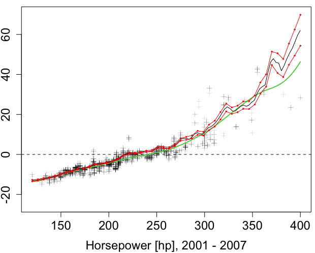
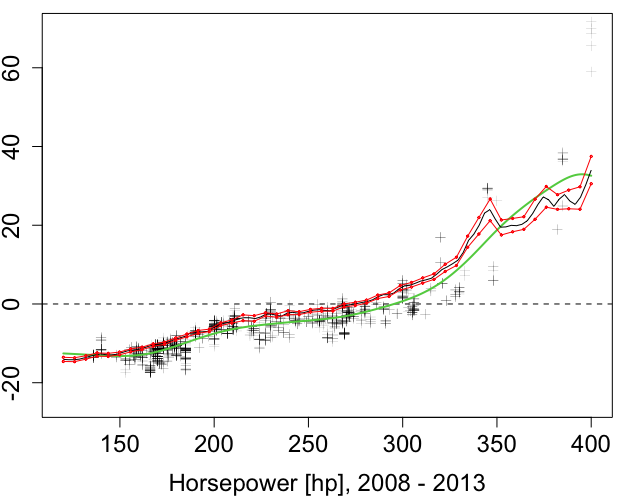
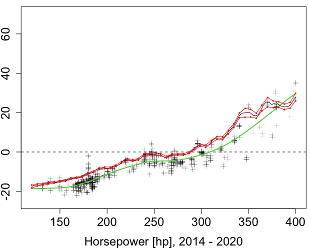
Figure 1: Estimated Shapley curves for horsepower in dependence of horsepower (in hp) for a vehicle length of $190$ inches and vehicle weight of $3500$ pounds. The time periods are 2001–2007, 2008–2013 and 2014–2020. Estimated SHAP values (black crosses) and smoothed curve based on these values (green curve).

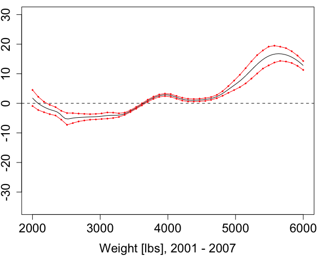
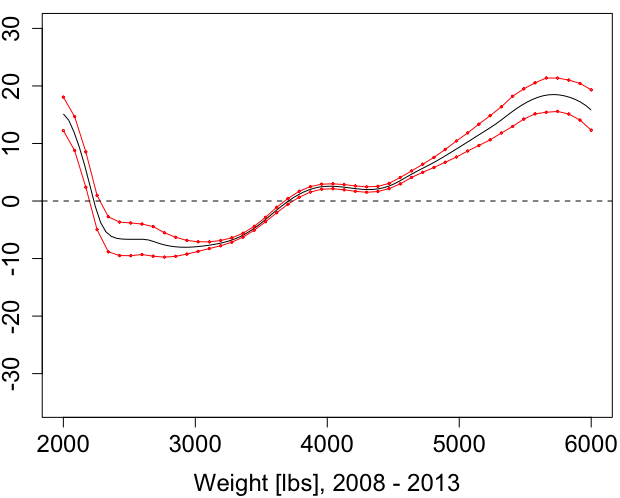
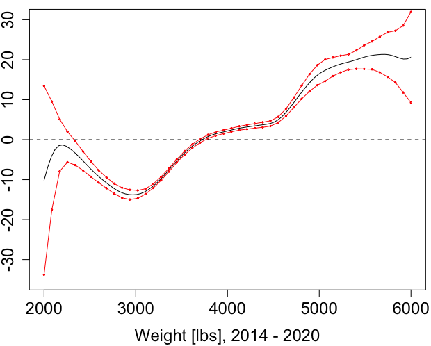
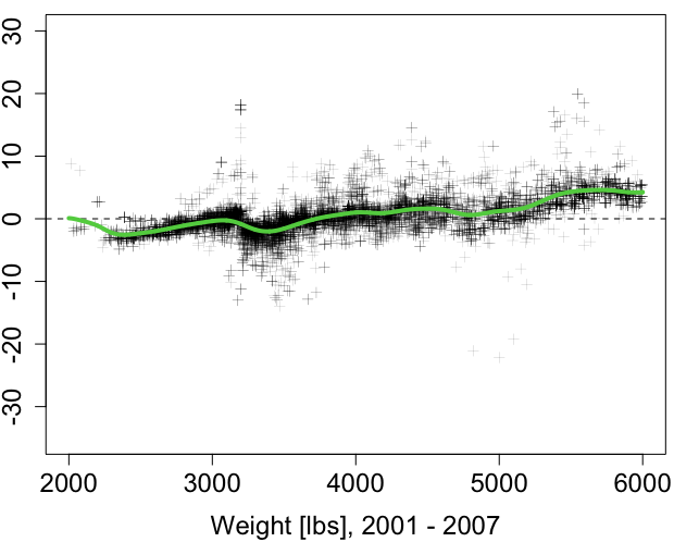
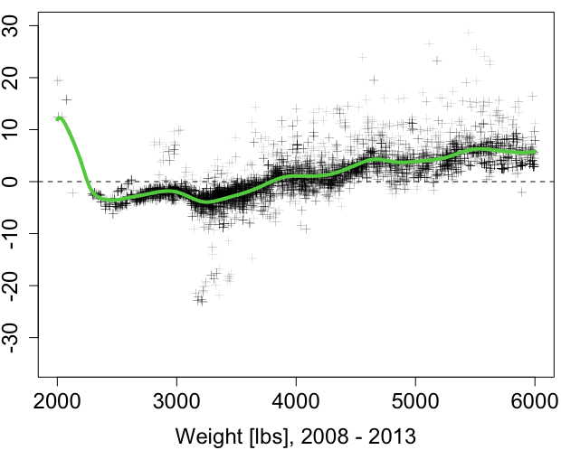
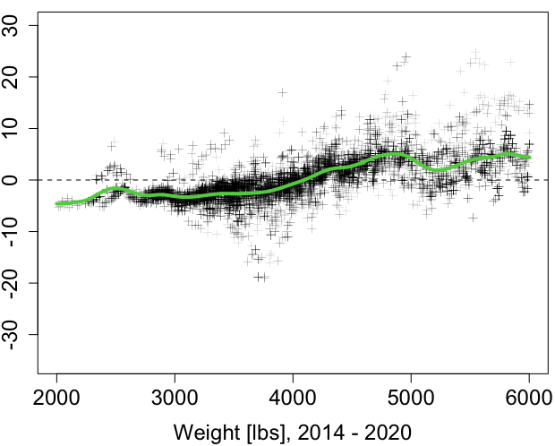
Figure 2: First row: Estimated Shapley curves for vehicle weight in dependence of weight (in lbs) for a vehicle length of $190$ inches and $190$ horsepower. The time periods are 2001–2007, 2008–2013 and 2014–2020. Second row: Estimated SHAP values (black crosses) and smoothed curve based on these values (green curve).

We now want to illustrate the results for the estimated confidence intervals for the Shapley Curves over the support of variable $j$. Therefore we fix the remaining variables at a value that lies in a dense area of the data or at the median. The results of this exercise are shown in Figure 2 for vehicle weight, in Figure 1 for horsepower and in the supplementary material for vehicle length. This type of analysis is not to be mistaken with the interpretation of confidence bands. For each ’slice plot’ we illustrate $\widehat{\phi}_{j}(x)$ against $X_{j}$. Figure 1 illustrates the Shapley curve as such a slice plot for the variable horsepower. Across the time domain, we infer that horsepower in general is contributing less to an increased price as we move from the first to the second and third time interval. This effect is especially prominent as we compare the first and second time interval. The reason is that as technology develops over time, it is less costly for car manufacturers to produce vehicles with higher horsepower. Further, we include estimated SHAP values, as well as a smoothed curve of these values. In order to make the comparison between Shapley curves and smoothed SHAP values as fair as possible, we estimate SHAP values for Horsepower, only on observations with realizations of Weight and a Length lying in an interval around the median. It shows that the Shapley curve for horsepower and the smoothed SHAP values result in similar curves in such a scenario. However, the smoothed SHAP curve is not accompanied by confidence intervals.

The Shapley curve for vehicle weight (Figure 2), shows that a lighter weight contributes to a price decrease, accompanied by stagnation at around 4000 lbs and an increase shortly after. Further, it shows that the Shapley curve is stretched apart on the tails across the time intervals. The estimated confidence intervals have a larger spread as we move to the tails of the variables. This is intuitive as we have more variation in price for the observations in this area. For example, a very heavy car with more than 5500 lbs can either be a Nissan NV Cargo Van or a Cadillac Escalade SUV. On the left tail, we observe insignificance for the third period. The second row in Figure 2 includes the SHAP values estimated for each observation in the respective time interval. In addition, we fit a smoother on these values, to make a comparison to our Shapley curves. In contrary to Figure 1, we are estimating the SHAP values for all observations. This illustrates the original approach of SHAP.

Further, we observe that the variable vehicle length (Figure S3 in supplementary material) mostly does not significantly contribute to the price prediction after a length of approximately 230 inches for the first and second time period. However, we observe a downward trend in the prices for longer cars the more recent the time interval is.

Finally, we are interested in the cumulative price contribution of the variables at hand. Therefore we sequentially accumulate the Shapley curves to the unconditional mean prediction, such that the additional contribution of a variable to the prediction is visible. For instance, the green area in Figure 3 indicates an increase in the price prediction, after adding up a certain variable. We call this the cumulative Shapley curves, which are a function of a single variable of interest, with fixed remaining variables.

For example, the first row of Figure 3 includes the cumulative Shapley curves as a function of horsepower for a car length of 190 inches and 3500 pounds. As we see, adding the curves for vehicle weight and length does barely contribute to the prediction of price. In other words, their importance as a function of horsepower is negligible. The second row of Figure 3 shows that as we include the second and third variable as a function of weight, we see that the price contribution mainly changes as we move closer to the tails. The first column of said figure indicates how much more the addition of horsepower explains price differences in comparison to the average prediction. If we plot it as a function of horsepower, it contributes a lot, which means the area is relatively large.

A similar argument holds for the Shapley curve for horsepower, as a function of weight. However, for the third variable the corresponding area is rather small. In general, we observe that even adding the Shapley curve for weight and length does not contribute a lot to the price prediction as a function of length.

A qualitative comparison can be made to the additive model. First, note that the first row suggests that the price contribution of weight and length does not depend on horsepower. Assume that the unknown data-generating process indeed follows an additive model as defined in Assumption 5. In that case Figure 3 would have relatively large areas in the diagonal plots and an almost non-existent area in the off-diagonals. We conclude that this graphical analysis of sequential Shapley curves enables a heuristic distinction to the additive model.

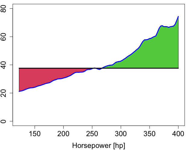
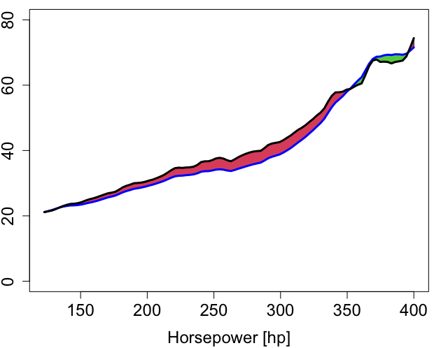
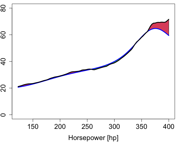
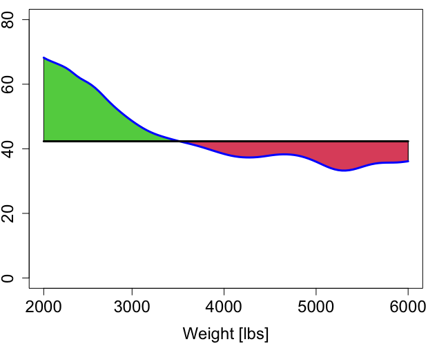
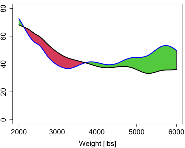
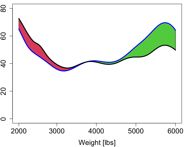
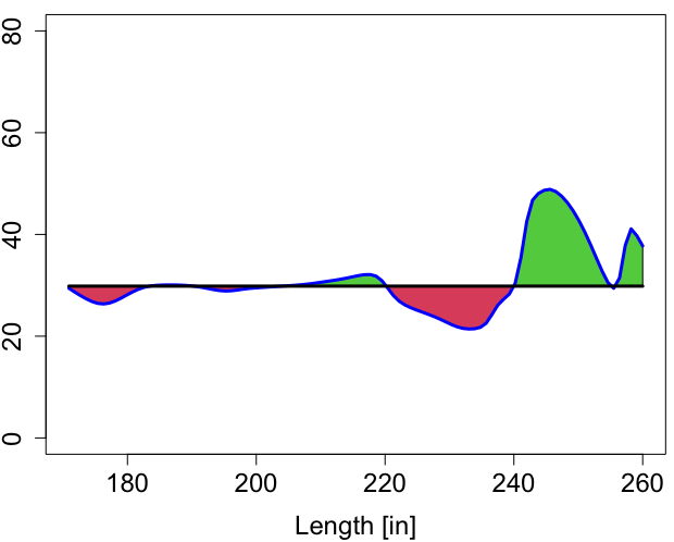
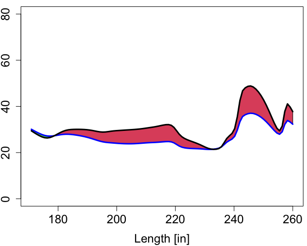
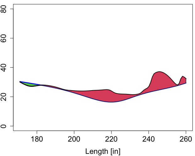
Figure 3: Cumulative Shapley Curves: Green area indicates an increase and red area indicates decrease in the price prediction of updated cumulative Shapley curve (in blue). Left panel shows $\bar{Y}$ in black and $\widehat{\phi}_{1}(x)+\bar{Y}$ in blue; Mid panel shows $\widehat{\phi}_{1}(x)+\bar{Y}$ in black and $\widehat{\phi}_{1}(x)+\widehat{\phi}_{2}(x)+\bar{Y}$ in blue; Right panel shows $\widehat{\phi}_{1}(x)+\widehat{\phi}_{2}(x)+\bar{Y}$ in black and $\widehat{\phi}_{1}(x)+\widehat{\phi}_{2}(x)+\widehat{\phi}_{3}(x)+\bar{Y}=\widehat{m}(x)$ in blue. The third plot in each row contains the conditional mean prediction in blue. First row for vehicles with weight of 3500 lbs and length of 190 inches. Second row for vehicles with horsepower of 250 and length of 190 inches. Third row for vehicles with horsepower of 250 lbs and weight of 3500 lbs.

6 Conclusion

This paper analyzes Shapley curves as a local measure of variable importance in a nonparametric framework. We give a rigorous definition of Shapley curves on the population level. As for estimation, we discuss two estimation strategies, the component-based approach, and the integration-based approach. We show that both estimators globally converge with the nonparametric rate of Stone (1982) to the population counterpart. Asymptotic normality is obtained for both estimators. We show that the asymptotic variance is identical for both approaches. However, the integration-based approach is accompanied by an inflated asymptotic bias. In our simulation exercise, this difference is visible in the results for the MISE. The advantage of the integration-based estimator is that only one pilot estimator is required to estimate the components. We show that our tailored wild bootstrap procedure is consistent and results in good finite sample coverage. Under the assumption of an additive model a one-dimensional convergence rate results for Shapley curves (Stone, 1985). For an extensive vehicle price data set we show that Shapley curves are a useful tool for the practitioner to gain insight into pricing and the importance of vehicle characteristics. The estimated confidence intervals enable to distinguish between significant and non-significant sections of the variables. Building on our results, empirical researchers as well as practitioners can conduct statistical inference for Shapley curves.

SUPPLEMENTAL: APPENDICES

This supplementary document is organized as follows. In Section A we provide proofs of Proposition 1, Theorem 2, Proposition 3 and Theorem 5. Intuition on the proposed bootstrap procedure for finite samples is given. In Section B we give details on the simulation procedure and include supporting tables and figures of the simulation exercise as well as the empirical application.

Appendix A Proofs

A.1 Proof of Proposition 1

Proof  Using the weighted sum representation (8) we write

$$\widehat{\phi}_{j}(x)-\phi_{j}(x)=\sum_{s\subseteq N}\omega_{j,s}\left\{\widehat{m}_{s}(x_{s})-m_{s}(x_{s})\right\}.$$

Taking the squared error and applying Jensen’s Inequality gives

$$\left\{\widehat{\phi}_{j}(x)-\phi_{j}(x)\right\}^{2} =\left[\sum_{s\subseteq N}\omega_{j,s}\left\{\widehat{m}_{s}(x_{s})-m_{s}(x_{s})\right\}\right]^{2}$$

$$\leq\sum_{s\subseteq N}\omega_{j,s}^{2}\left\{\widehat{m}_{s}(x_{s})-m_{s}(x_{s})\right\}^{2}.$$

Next, we integrate over $\mathcal{X}$ resulting in

$$\int_{\mathcal{X}}\left\{\widehat{\phi}_{j}(x)-\phi_{j}(x)\right\}^{2}dx\leq\sum_{s\subseteq N}\omega_{j,s}^{2}\int_{\mathcal{X}}\left\{\widehat{m}_{s}(x_{s})-m_{s}(x_{s})\right\}^{2}dx.$$

Finally, taking the expectation gives the MISE

$${\sf E}\left[\int_{\mathcal{X}}\left\{\widehat{\phi}_{j}(x)-\phi_{j}(x)\right\}^{2}dx\right] \leq\sum_{s\subseteq N}\omega_{j,s}^{2}{\sf E}\left[\int_{\mathcal{X}}\left\{\widehat{m}_{s}(x_{s})-m_{s}(x_{s})\right\}^{2}dx\right]$$

$$=\sum_{s\subseteq N}\omega_{j,s}^{2}\text{MISE}\left\{\widehat{m}_{s}(x_{s}),m_{s}(x_{s})\right\}.$$

By Assumptions 1, 2 and 3, $m_{s}(x_{s})$ belongs to the class of $|s|$-dimensional twice continuously differentiable functions. By choosing the bandwidth as $h_{s}\sim n^{-\frac{1}{4+|s|}}$ and invoking Theorem 2 of Fan (1993) one sees that the estimator achieves the minimax rate of Stone (1982):

$$\text{MISE}\left\{\widehat{m}_{s}(x_{s}),m_{s}(x_{s})\right\}=\mathcal{O}\left(n^{-\frac{4}{4+|s|}}\right).$$ (S1)

Therefore,

$${\sf E}\left[\int_{x}\left\{\widehat{\phi}_{j}(x)-\phi_{j}(x)\right\}^{2}dx\right] \leq\sum_{s\subseteq N}\omega_{j,s}^{2}\mathcal{O}\left(n^{-\frac{2p}{4+|s|}}\right)$$

$$=\mathcal{O}\left(n^{-\frac{4}{4+d}}\right)+{\scriptstyle\mathcal{O}}\left(n^{-\frac{4}{4+d}}\right).$$

 

A.2 Proof of Theorem 2

Proof  Let $h_{m}$ be the optimal bandwidth of the $d$-dimensional model and let $\frac{1}{d}$ denote the corresponding weight of the $d$-dimensional model. From the proof of Proposition 1 it follows that

$$\widehat{\phi}_{j}(x)-\phi_{j}(x)=\frac{1}{d}(\widehat{m}(x)-m(x))+{\scriptstyle\mathcal{O}}_{p}\left(n^{-\frac{2}{4+d}}\right).$$

Asymptotic normality follows by Assumptions 1, 2 and 3 and the Lindeberg-Feller Central Limit Theorem (CLT),

$$\sqrt{nh_{m}^{d}}(\widehat{\phi}_{j}(x)-\phi_{j}(x))\stackrel{{\scriptstyle\mathcal{L}}}{{\rightarrow}}N\left(B(x),V(x)\right),$$

where the asymptotic bias $B(x)$ and asymptotic variance $V(x)$ are given in Theorem 2.1 of Ruppert and Wand (1994),

$$B(x) =\frac{1}{d}\frac{\mu_{2}(k)}{2}\sum^{d}_{j=1}\frac{\partial^{2}m(x)}{\partial^{2}x_{j}},$$

$$V(x) =\frac{1}{d^{2}}||k||^{2}_{2}\frac{\sigma^{2}(x)}{f(x)}.$$

 

A.3 Proof of Proposition 3

Proof  In order to prove the consistency of the bootstrap procedure, we need to show that

$$\bigg{\lvert}P^{Y\mid X}\left[\sqrt{nh_{m}^{d}}\left\{\widehat{\phi}_{j}(x)-\phi_{j}(x)\right\}<z\right]-\Phi_{B,V}(z)\bigg{|}{\rightarrow}0,$$ (S2)

and

$$\bigg{\lvert}P^{*}\left[\sqrt{nh_{m}^{d}}\left\{\widehat{\phi}^{*}_{j}(x)-\widehat{\phi}_{g,j}(x)\right\}<z\right]-\Phi_{B,V}(z)\bigg{|}{\rightarrow}0,$$ (S3)

where $\Phi_{B,V}(z)$ denotes a normal distribution with mean $B(x)$ and covariance $V(x)$ as defined in Theorem 2. To show (S2), we follow the proof of Lemma 1 of Härdle and Marron (1991) by noting that,

$$\sqrt{nh^{d}_{m}}\left\{\widehat{\phi}_{j}(x)-\phi_{j}(x)\right\} =\sqrt{nh^{d}_{m}}\frac{1}{d}\left\{\widehat{m}(x)-m(x)\right\}+{\scriptstyle\mathcal{O}}_{p}\left(1\right)$$ (S4)

$$=L_{n}+{\scriptstyle\mathcal{O}}_{p}(L_{n}),$$

where $L_{n}=\frac{1}{d}\sqrt{nh^{d}_{m}}\left[\frac{1}{n}\sum^{n}_{i=1}\frac{K_{h}(x-X_{i})\left\{Y_{i}-m(x)\right\}}{f(x)}\right]$ as in Linton and Nielsen (1995). Denote $W^{{}^{\prime}}_{i}(x)=\sqrt{\frac{h^{d}_{m}}{n}}\frac{K_{h}(x-X_{i})}{f(x)}$, then we can further decompose $L_{n}$ into a bias and a variance term, $L_{n}=B_{n}+V_{n}$ with

$$B_{n} =\sum_{i=1}^{n}W_{i}^{{}^{\prime}}(x)\left(m(X_{i})-m(x)\right),$$

$$V_{n} =\sum_{i=1}^{n}W_{i}^{{}^{\prime}}(x)\varepsilon_{i}.$$

While we have $B_{n}\stackrel{{\scriptstyle p}}{{\rightarrow}}B(x)$, looking at the second and third moment of $V_{n}$, conditional on $X_{1},\ldots,X_{n}$,

$$S_{2n}=\sum^{n}_{i=1}\text{Var}\left\{W^{{}^{\prime}}_{i}(x)\varepsilon_{i}\lvert X_{1},\ldots,X_{n}\right\}=\mathcal{O}(1)$$

and by Assumption 4,

$$S_{3n}=\sum^{n}_{i=1}{\sf E}\left\{\lvert W^{{}^{\prime}}_{i}(x)\varepsilon_{i}\lvert^{3}\lvert X_{1},\ldots,X_{n}\right\}=\mathcal{O}\left(\frac{1}{\sqrt{nh}}\right).$$

We can apply Theorem 3 on page 111 in Petrov (1975), the Esseen’s inequality for arbitrary independent random variables, to bound (S2) by noting,

$$\frac{S_{3n}}{S^{\frac{3}{2}}_{2n}}={\scriptstyle\mathcal{O}}(1)\ \text{a.s.}$$

To prove (S4), we have to obtain a similar bound for the bootstrap version of the estimator. Note that

$$\sqrt{nh^{d}_{m}}\left\{\widehat{\phi}^{*}_{j}(x)-\widehat{\phi}_{g,j}(x)\right\} =\sqrt{nh^{d}_{m}}\frac{1}{d}\left\{\widehat{m}^{*}(x)-\widehat{m}_{g}(x)\right\}+{\scriptstyle\mathcal{O}}_{p}\left(1\right),$$

which is a similar starting argument as in the proof of (S3). The remaining steps follow by Lemma 2 of Härdle and Marron (1991).

 

A.4 Intuition on the wild bootstrap adjustment

We want to provide some intuition for including the lower order terms in the bootstrap algorithm. Recall that $\widehat{\phi}^{*}_{j}(x)=\sum_{s\subseteq N}\omega_{j,s}\widehat{m}^{*}_{s}(x_{s})$ and $\widehat{\phi}_{j,g}(x)=\sum_{s\subseteq N}\omega_{j,s}\widehat{m}_{s,g}(x_{s})$. Let $W_{s,i}(x_{s})$ denote the local linear weights for $\widehat{m}_{s}(x_{s})$. It can be shown that

$$\widehat{\phi}_{j}(x)-\phi_{j}(x) \approx\sum^{n}_{i=1}\left\{\sum_{s\subseteq N}W_{s,i}(x_{s})\omega_{j,s}\varepsilon_{s,i}\right\}$$ (S5)

$$\widehat{\phi}^{*}_{j}(x)-\widehat{\phi}_{j,g}(x) \approx\sum^{n}_{i=1}\left\{\sum_{s\subseteq N}W_{s,i}(x_{s})\omega_{j,s}\widehat{\varepsilon}_{s,i}\right\}V_{i}.$$ (S6)

The conditional variances of (S5) and (S6) are given by

$$\text{Var}(\widehat{\phi}_{j}(x)-\phi_{j}(x)\lvert X) =\sum^{n}_{i=1}\sum_{s\in\mathcal{S}}\sum_{s^{{}^{\prime}}\in\mathcal{S}}\omega_{j,s}\omega_{j,s^{{}^{\prime}}}W_{s,i}(x_{s})W_{s^{{}^{\prime}},i}(x_{s}){\sf E}(\varepsilon_{s,i}\varepsilon_{s^{{}^{\prime}},i}\lvert X)$$ (S7)

$$\text{Var}(\widehat{\phi}^{*}_{j}(x)-\widehat{\phi}_{j,g}(x)\lvert X) =\sum^{n}_{i=1}\sum_{s\in\mathcal{S}}\sum_{s^{{}^{\prime}}\in\mathcal{S}}\omega_{j,s}\omega_{j,s^{{}^{\prime}}}W_{s,i}(x_{s})W_{s^{{}^{\prime}},i}(x_{s}){\sf E}(\widehat{\varepsilon}_{s,i}\widehat{\varepsilon}_{s^{{}^{\prime}},i}\lvert X){\sf E}(V^{2}_{i}).$$ (S8)

Asymptotically, the leading terms in the conditional variance expressions are

$$\text{Var}(\widehat{\phi}_{j}(x)-\phi_{j}(x)\lvert X) =\sum^{n}_{i=1}\frac{1}{d^{2}}W_{m,i}^{2}(x){\sf E}(\varepsilon^{2}_{i}\lvert X)+{\scriptstyle\mathcal{O}}\left(n^{-\frac{4}{4+d}}\right)$$

$$\text{Var}(\widehat{\phi}^{*}_{j}(x)-\widehat{\phi}_{j,g}(x)\lvert X) =\sum^{n}_{i=1}\frac{1}{d^{2}}W_{m,i}^{2}(x){\sf E}(\widehat{\varepsilon}^{2}_{i}\lvert X)+{\scriptstyle\mathcal{O}}\left(n^{-\frac{4}{4+d}}\right).$$

While not relevant for the asymptotic results, the smaller order terms in (S7) and (S8) can play an important role in finite samples. Including these terms will lead to a more accurate reflection of the variance by the bootstrap procedure. As we see, the variance terms (S7) and (S8) are similar, given that ${\sf E}(\varepsilon_{s,i}\varepsilon_{s^{{}^{\prime}},i}\lvert X)\approx{\sf E}(\widehat{\varepsilon}_{s,i}\widehat{\varepsilon}_{s^{{}^{\prime}},i}\lvert X)$ and ${\sf E}(V^{2}_{i})=1$.

A.5 Proof of Theorem 5

Proof  Let $h_{m}\sim n^{-\frac{1}{4+d}}$ and under Assumptions 1, 2 and 3 it follows that

$$\text{MISE}\left\{\widetilde{m}(x),m(x)\right\}=\mathcal{O}\left(n^{-\frac{4}{4+d}}\right).$$

The uniform convergence of $\widetilde{m}_{s}(x_{s})$ results directly from the continuous mapping theorem (CMT), such that

$$\text{MISE}\left\{\widetilde{\phi}_{j}(x),\phi_{j}(x)\right\}=\mathcal{O}\left(n^{-\frac{4}{4+d}}\right).$$ (S9)

Next, we prove asymptotic normality of $\widetilde{m}_{s}(x_{s})$. Similar to the proof of Theorem 2, the weighted sum representation leads to

$$\widetilde{\phi}_{j}(x)-\phi_{j}(x) =\sum_{s\subseteq N}\omega_{j,s}\left\{\widetilde{m}_{s}(x_{s})-m_{s}(x_{s})\right\}.$$

By Assumptions 1,2 and 3, the Lindeberg-Feller central limit theorem and the continuous mapping theorem it follows that

$$\sqrt{nh_{m}^{d}}\sum_{s\subseteq N}\omega_{j,s}\left\{\widetilde{m}_{s}(x_{s})-m_{s}(x_{s})\right\}\stackrel{{\scriptstyle\mathcal{L}}}{{\rightarrow}}N\left(B_{int}(x),V(x)\right),$$

where the asymptotic bias $B_{int}(x)$ and the asymptotic variance $V(x)$ are

$$B_{int}(x) =\frac{\mu_{2}(k)}{2}\sum_{s\subseteq N}\omega_{j,s}\left\{\sum^{d}_{j=1}\int_{X_{-s}}\frac{\partial^{2}m(x)}{\partial^{2}x_{j}}f_{X_{-s}|X_{s}}(x_{-s}|x_{s})dx_{-s}\right\},$$

$$V(x) =\frac{1}{d^{2}}||k||^{2}_{2}\frac{\sigma^{2}(x)}{f(x)}.$$

The bias accumulates as the conditional mean for each subset converges at the same rate to the population counterpart, whereas the variance is the same as for the component-based estimator. We prove both in the following.

First, we derive the bias of the integration-based estimator. By using the weighted sum representation we get

$${\sf E}\left\{\widetilde{\phi}_{j}(x)\right\}-\phi_{j}(x)=\sum_{s\subseteq N}\omega_{j,s}\left[{\sf E}\left\{\widetilde{m}_{s}(x_{s})\right\}-m_{s}(x_{s})\right].$$ (S10)

Similar to Linton and Nielsen (1995), by Assumptions 1,2 and 3 the bias of the integration-based estimator of the subset $s$, $\widetilde{m}_{s}(x_{s})$, is given as

$${\sf E}\left\{\widetilde{m}_{s}(x_{s})\right\}-m_{s}(x_{s})\approx h_{m}^{2}\mu_{2}(k)\frac{1}{2}\left\{\sum^{d}_{j=1}\int_{X_{-s}}\frac{\partial^{2}m(x)}{\partial^{2}x_{j}}dF_{X_{-s}|X_{s}}(x_{-s}|x_{s})\right\}.$$ (S11)

The result follows as we insert (S11) into (S10).

Next, we derive the asymptotic variance of the integration-based estimator. Under Assumptions 1,2 and 3 we show that:

$$\text{Var}\left\{\widetilde{\phi}_{j}(x)\right\}=\frac{1}{d^{2}}\text{Var}\left\{\widetilde{m}(x)\right\}+{\scriptstyle\mathcal{O}}\left(\frac{1}{nh_{m}^{d}}\right).$$ (S12)

We use the results of Linton and Nielsen (1995) to derive the asymptotic variance of the integration-based estimator for a given component function. The key idea is to consider the variance of the internal estimator (estimator with known density) and show that the difference of this internal estimator and the local linear estimator is of smaller order. In contrast to Linton and Nielsen (1995), the proof also works for dimension $d>2$. The reason is that the difference between the internal estimator and the local linear estimator is of small order for any dimension $d$, namely $\mathcal{O}_{p}(n^{-1}h_{m}^{-d})+{\scriptstyle\mathcal{O}}_{p}(h_{m}^{d})$.

As a consequence the variance of $\widetilde{m}_{s}(x_{s})$, for $|s|<d$, is given by

$$\text{Var}\left\{\widetilde{m}_{s}(x_{s})\right\} \approx\frac{1}{nh_{m}^{|s|}}\|k\|^{2}_{2}\int\frac{\sigma^{2}(x)f^{2}_{X_{-s}|X_{s}}(x_{-s}|x_{s})}{f(x)}dx_{-s}$$

$$=\mathcal{O}\left(\frac{1}{nh_{m}^{\lvert s\rvert}}\right)={\scriptstyle\mathcal{O}}\left(\frac{1}{nh_{m}^{d}}\right).$$

Equation (S12) follows directly, since the variance of the lower dimensional components as well as the covariance terms converge at a faster rate than the variance of the $d$-dimensional model.

 

Appendix B Simulation Details, Tables and Plots

The coverage probability in Table 2 is estimated for $\alpha=0.05,0.1$ and $0.15$ for increasing sample size. First, we simulate data following (15) with additional Gaussian noise. The proposed bootstrap procedure is conducted as described in Section 3.1. We estimate $\widehat{\phi}^{b}_{j}(x_{s})$ at the point $(-0.5,-0.5)$. The procedure is repeated in $B=1000$ replications, where we estimate the component-based Shapley curve for each replication $b=1,\ldots,B$. We choose the bandwidth $g_{s}=h_{s}\times\log(\log(n))\times 4$ such that $\frac{h_{s}}{g_{s}}\rightarrow 0$ as $n\rightarrow\infty$ for all subsets $s\in\mathcal{S}$.

The integral within the MISE is approximated with the cubature R package, which adaptively calculates the multidimensional integral over hypercubes.

Table 3: MISE of Shapley Curves for component-based estimator $\widehat{\phi}_{j}$ and integration-based estimator $\widetilde{\phi}_{j}$ for each variable. An additive and non-linear DGP is used for $\rho=0$ and $\rho=0.8$. The error terms follow $\varepsilon\sim\operatorname{t}(5)$.

DGP	$\rho$	$n$	$\widehat{\phi}_{1}$	$\widetilde{\phi}_{1}$	$\widehat{\phi}_{2}$	$\widetilde{\phi}_{2}$	$\widehat{\phi}_{3}$	$\widetilde{\phi}_{3}$
Additive	$0$	300	10.99	20.05	10.17	9.71	3.06	0.44
		500	5.96	7.95	6.38	8.40	2.02	0.28
		1000	3.71	4.41	4.30	5.41	1.09	0.16
		2000	2.26	2.65	2.63	3.34	0.62	0.09
	$0.8$	300	9.13	10.57	9.88	11.45	3.10	1.81
		500	6.39	7.14	6.76	7.95	2.12	1.19
		1000	4.32	4.56	4.38	5.03	1.44	0.73
		2000	2.84	2.91	2.86	3.26	0.93	0.45
Non-linear	$0$	300	11.48	17.13	15.25	20.06	2.37	0.57
		500	7.25	10.04	8.43	10.29	1.03	0.32
		1000	4.15	5.73	4.93	6.04	0.56	0.18
		2000	2.46	3.41	2.85	3.62	0.34	0.11
	$0.8$	300	12.60	14.84	14.82	17.38	3.61	2.44
		500	9.35	10.35	9.77	12.24	2.64	1.71
		1000	6.07	6.06	5.98	7.53	1.78	1.05
		2000	4.04	3.82	3.77	4.73	1.22	0.68

Table 4: Summary statistics

	Mean	Min	$q_{0.25}$	$q_{0.5}$	$q_{0.75}$	Max
Horsepower	258	70	181	260	310	808
Weight [lbs]	4233	1808	3322	3970	5042	8039
Length [in]	199	106	180	192	219	290
Price [1000 USD]	36.35	8.9	24.1	31.23	41.19	191.5

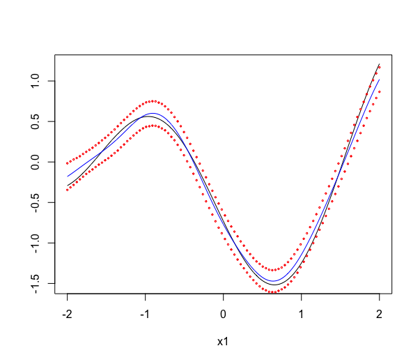
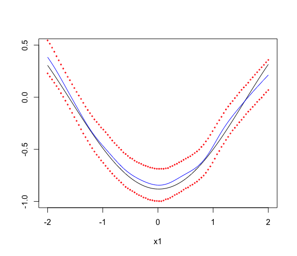
Figure 4: Population Shapley Curve (black) and componend-based estimated Shapley Curve (blue) with $95\%$ bootstrap confidence intervals (red) for the first variable (left) and second variable (right). $x_{1}$ varies on [-2,2] and $x_{2}=-0.5$. The DGP is $m(x)=-\text{sin}(2x_{1})+\text{cos}(3x_{2})+2\text{cos}(x_{1})\text{sin}(2x_{2})$ with Gaussian error terms. $B=10000$ bootstrap replications and $n=2000$.

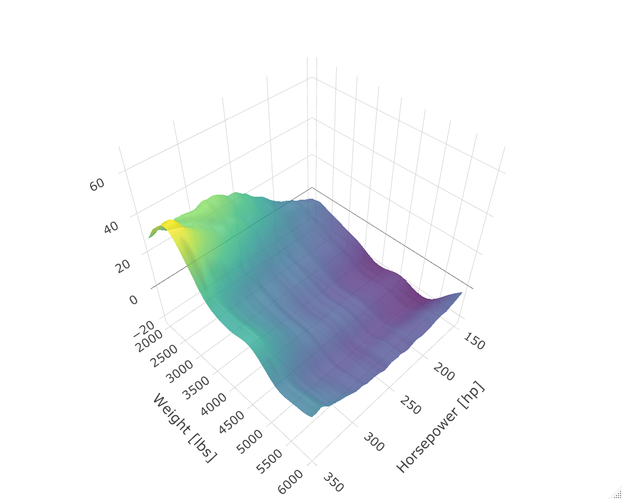
Figure 5: Estimated Shapley curve for horsepower in dependence of vehicle weight (in lbs) and horsepower (in hp) for a vehicle length of $190$ inches for the pooled data set from year 2001–2020.

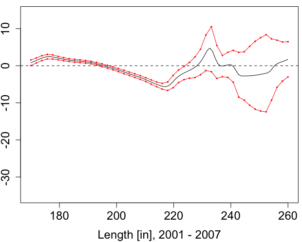
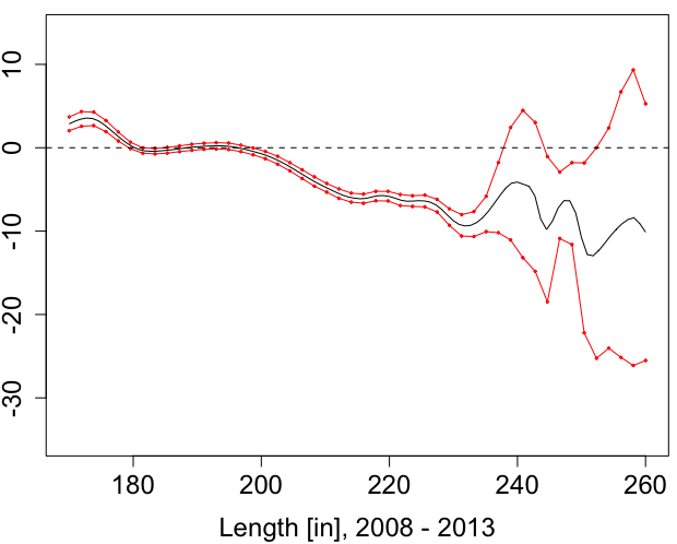
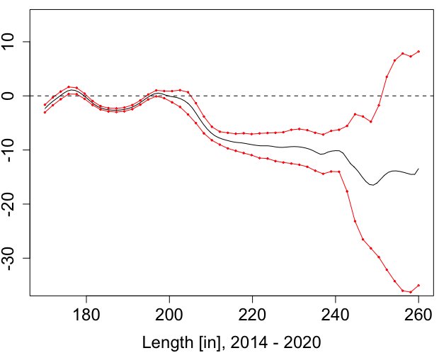
Figure 6: Estimated Shapley curves for vehicle length in dependence of length (in) for a vehicle weight of $3500$ pounds and horsepower of $190$. The time periods are 2001–2007, 2008–2013 and 2014–2020.

References

- Aas et al. [2021] Kjersti Aas, Thomas Nagler, Martin Jullum, and Anders Løland. Explaining predictive models using shapley values and non-parametric vine copulas. Dependence Modeling, 9(1):62–81, 2021.
- Aldrich [1995] John Aldrich. Correlations genuine and spurious in pearson and yule. Statistical science, pages 364–376, 1995.
- Auestad and Tjøstheim [1991] Bjørn Auestad and Dag Tjøstheim. Functional identification in nonlinear time series. In Nonparametric Functional Estimation and Related Topics, pages 493–507. Springer, 1991.
- Bénard et al. [2022a] Clément Bénard, Gérard Biau, Sébastien Da Veiga, and Erwan Scornet. Shaff: Fast and consistent shapley effect estimates via random forests. In International Conference on Artificial Intelligence and Statistics, pages 5563–5582. PMLR, 2022a.
- Bénard et al. [2022b] Clément Bénard, Sébastien Da Veiga, and Erwan Scornet. Mean decrease accuracy for random forests: inconsistency, and a practical solution via the sobol-mda. Biometrika, 2022b.
- Berman et al. [2012] Steve Berman, Leandro DalleMule, Michael Greene, and John Lucker. Simpson’s paradox: A cautionary tale in advanced analytics. Significance, 2012.
- Buja et al. [1989] Andreas Buja, Trevor Hastie, and Robert Tibshirani. Linear smoothers and additive models. The Annals of Statistics, pages 453–510, 1989.
- Chen et al. [1996] Richel Chen, Wolfgang Härdle, Oliver B Linton, and E Severance-Lossin. Nonparametric estimation of additive separable regression models. In Statistical Theory and Computational Aspects of Smoothing, pages 247–265. Springer, 1996.
- Covert et al. [2020] Ian Covert, Scott M Lundberg, and Su-In Lee. Understanding global feature contributions with additive importance measures. Advances in Neural Information Processing Systems, 33:17212–17223, 2020.
- Covert et al. [2021] Ian Covert, Scott Lundberg, and Su-In Lee. Explaining by removing: A unified framework for model explanation. Journal of Machine Learning Research, 22(209):1–90, 2021.
- Dagenais [1969] Marcel G Dagenais. A threshold regression model. Econometrica, 37(2):193–203, 1969.
- Durlauf and Johnson [1995] Steven N Durlauf and Paul A Johnson. Multiple regimes and cross-country growth behaviour. Journal of applied econometrics, 10(4):365–384, 1995.
- Fan [1993] Jianqing Fan. Local linear regression smoothers and their minimax efficiencies. The annals of Statistics, pages 196–216, 1993.
- Fan et al. [1998] Jianqing Fan, Wolfgang Härdle, and Enno Mammen. Direct estimation of low-dimensional components in additive models. The Annals of Statistics, 26(3):943–971, 1998.
- Hansen [2000] Bruce E Hansen. Sample splitting and threshold estimation. Econometrica, 68(3):575–603, 2000.
- Härdle and Mammen [1993] Wolfgang Härdle and Enno Mammen. Comparing nonparametric versus parametric regression fits. The Annals of Statistics, pages 1926–1947, 1993.
- Härdle and Marron [1991] Wolfgang Härdle and James Stephen Marron. Bootstrap simultaneous error bars for nonparametric regression. The Annals of Statistics, pages 778–796, 1991.
- Härdle et al. [2004] Wolfgang Härdle, Marlene Müller, Stefan Sperlich, Axel Werwatz, et al. Nonparametric and semiparametric models. Springer, 2004.
- Hiabu et al. [2023] Munir Hiabu, Joseph T Meyer, and Marvin N Wright. Unifying local and global model explanations by functional decomposition of low dimensional structures. In International Conference on Artificial Intelligence and Statistics, pages 7040–7060. PMLR, 2023.
- Li et al. [2022] Wei Li, Wolfgang Karl Härdle, and Stefan Lessmann. A data-driven case-based reasoning in bankruptcy prediction. arXiv preprint arXiv:2211.00921, 2022.
- Linton and Nielsen [1995] Oliver Linton and Jens Perch Nielsen. A kernel method of estimating structured nonparametric regression based on marginal integration. Biometrika, pages 93–100, 1995.
- Linton et al. [1997] Oliver B Linton, Rong Chen, Naiysin Wang, and Wolfgang Härdle. An analysis of transformations for additive nonparametric regression. Journal of the American Statistical Association, 92(440):1512–1521, 1997.
- Lundberg and Lee [2017] Scott M Lundberg and Su-In Lee. A unified approach to interpreting model predictions. In Proceedings of the 31st international conference on neural information processing systems, pages 4768–4777, 2017.
- Lundberg et al. [2020] Scott M Lundberg, Gabriel Erion, Hugh Chen, Alex DeGrave, Jordan M Prutkin, Bala Nair, Ronit Katz, Jonathan Himmelfarb, Nisha Bansal, and Su-In Lee. From local explanations to global understanding with explainable ai for trees. Nature machine intelligence, 2(1):56–67, 2020.
- Mammen [1992] Enno Mammen. Bootstrap, wild bootstrap, and asymptotic normality. Probability Theory and Related Fields, 93(4):439–455, 1992.
- Mammen [1993] Enno Mammen. Bootstrap and wild bootstrap for high dimensional linear models. The annals of statistics, 21(1):255–285, 1993.
- Mammen et al. [1999] Enno Mammen, Oliver Linton, and Jens Perch Nielsen. The existence and asymptotic properties of a backfitting projection algorithm under weak conditions. The Annals of Statistics, 27(5):1443–1490, 1999.
- Moawad et al. [2021] Ayman Moawad, Ehsan Islam, Namdoo Kim, Ram Vijayagopal, Aymeric Rousseau, and Wei Biao Wu. Explainable ai for a no-teardown vehicle component cost estimation: A top-down approach. IEEE Transactions on Artificial Intelligence, 2(2):185–199, 2021.
- Molnar et al. [2020] Christoph Molnar, Giuseppe Casalicchio, and Bernd Bischl. Interpretable machine learning–a brief history, state-of-the-art and challenges. In Joint European Conference on Machine Learning and Knowledge Discovery in Databases, pages 417–431. Springer, 2020.
- Newey [1994] Whitney K Newey. Kernel estimation of partial means and a general variance estimator. Econometric Theory, 10(2):1–21, 1994.
- Nielsen and Linton [1998] Jens Perch Nielsen and OB Linton. An optimization interpretation of integration and back-fitting estimators for separable nonparametric models. Journal of the Royal Statistical Society: Series B (Statistical Methodology), 60(1):217–222, 1998.
- Owen and Prieur [2017] Art B Owen and Clémentine Prieur. On shapley value for measuring importance of dependent inputs. SIAM/ASA Journal on Uncertainty Quantification, 5(1):986–1002, 2017.
- Petrov [1975] Valentin V. Petrov. Chapter v. In Sums of Independent Random Variables. Springer, New York, 1975.
- Ruppert and Wand [1994] David Ruppert and Matthew P Wand. Multivariate locally weighted least squares regression. The annals of statistics, pages 1346–1370, 1994.
- Schmidt-Hieber [2020] Johannes Schmidt-Hieber. Nonparametric regression using deep neural networks with relu activation function. The Annals of Statistics, 48(4):1875–1897, 2020.
- Scornet [2023] Erwan Scornet. Trees, forests, and impurity-based variable importance in regression. Annales de l’Institut Henri Poincare (B) Probabilites et statistiques, 59(1):21–52, 2023.
- Shapley [1953] Lloyd S Shapley. A value for n-person games. Contributions to the Theory of Games, 28(2):307–317, 1953.
- Stone [1982] Charles J Stone. Optimal global rates of convergence for nonparametric regression. The Annals of statistics, pages 1040–1053, 1982.
- Stone [1985] Charles J Stone. Additive regression and other nonparametric models. The Annals of Statistics, pages 689–705, 1985.
- Sundararajan and Najmi [2020] Mukund Sundararajan and Amir Najmi. The many shapley values for model explanation. In International conference on machine learning, pages 9269–9278. PMLR, 2020.
- Tjøstheim and Auestad [1994] Dag Tjøstheim and Bjørn H Auestad. Nonparametric identification of nonlinear time series: projections. Journal of the American Statistical Association, 89(428):1398–1409, 1994.
- Williamson and Feng [2020] Brian Williamson and Jean Feng. Efficient nonparametric statistical inference on population feature importance using shapley values. In International Conference on Machine Learning, pages 10282–10291. PMLR, 2020.