Fuzzy hyperspheres via confining potentials and energy cutoffs

Abstract

We simplify and complete the construction of fully $O(D)$-equivariant fuzzy spheres $S^{d}_{\Lambda}$, for all dimensions $d\equiv D-1$, initiated in [G. Fiore, F. Pisacane, J. Geom. Phys. 132 (2018), 423-451]. This is based on imposing a suitable energy cutoff on a quantum particle in $\mathbb{R}^{D}$ subject to a confining potential well $V(r)$ with a very sharp minimum on the sphere of radius $r=1$; the cutoff and the depth of the well diverge with $\Lambda\in\mathbb{N}$. As a result, the noncommutative Cartesian coordinates $\overline{x}^{i}$ generate the whole algebra of observables ${\cal A}_{\Lambda}$ on the Hilbert space ${\cal H}_{\Lambda}$; applying polynomials in the $\overline{x}^{i}$ to any ${\bm{\psi}}\in{\cal H}_{\Lambda}$ we recover the whole ${\cal H}_{\Lambda}$. The commutators of the $\overline{x}^{i}$ are proportional to the angular momentum components, as in Snyder noncommutative spaces. $\mathcal{H}_{\Lambda}$, as carrier space of a reducible representation of $O(D)$, is isomorphic to the space of harmonic homogeneous polynomials of degree $\Lambda$ in the Cartesian coordinates of (commutative) $\mathbb{R}^{D+1}$, which carries an irreducible representation ${\bm{\pi}}_{\Lambda}$ of $O(D\!+\!1)\supset O(D)$. Moreover, ${\cal A}_{\Lambda}$ is isomorphic to ${\bm{\pi}}_{\Lambda}\left(Uso(D\!+\!1)\right)$. We resp. interpret $\{{\cal H}_{\Lambda}\}_{\Lambda\in\mathbb{N}}$, $\{{\cal A}_{\Lambda}\}_{\Lambda\in\mathbb{N}}$ as fuzzy deformations of the space ${\cal H}_{s}:={\cal L}^{2}(S^{d})$ of (square integrable) functions on $S^{d}$ and of the associated algebra ${\cal A}_{s}$ of observables, because they resp. go to ${\cal H}_{s},{\cal A}_{s}$ as $\Lambda$ diverges (with $\hbar$ fixed). With suitable $\hbar=\hbar(\Lambda)\stackrel{{\scriptstyle\Lambda\to\infty}}{{\longrightarrow}}0$, in the same limit ${\cal A}_{\Lambda}$ goes to the (algebra of functions on the) Poisson manifold $T^{*}S^{d}$; more formally, $\{{\cal A}_{\Lambda}\}_{\Lambda\in\mathbb{N}}$ yields a fuzzy quantization of a coadjoint orbit of $O(D\!+\!1)$ that goes to the classical phase space $T^{*}S^{d}$.

1 Introduction

Noncommutative space(time) algebras are introduced and studied with various motivations, notably to provide an arena for   regularizing ultraviolet (UV) divergences in quantum field theory (QFT) (see e.g. [1]),  reconciling Quantum Mechanics and General Relativity in a satisfactory Quantum Gravity (QG) theory (see e.g. [2]),  unifying fundamental interactions (see e.g. [3, 4]). Noncommutative Geometry (NCG) [5, 8, 6, 7] has become a sophisticated framework that develops the whole machinery of differential geometry on noncommutative spaces. Fuzzy spaces are particularly appealing noncommutative spaces: a fuzzy space is a sequence $\{\mathcal{A}\}_{n\in\mathbb{N}}$ of finite-dimensional algebras such that $\mathcal{A}_{n}\overset{n\rightarrow\infty}{\longrightarrow}\mathcal{A}\!\equiv$algebra of regular functions on an ordinary manifold, with  $dim(\mathcal{A}_{n})\overset{n\rightarrow\infty}{\longrightarrow}\infty$. They have raised a big interest in the high energy physics community as a non-perturbative technique in QFT based on a finite discretization of space(time) alternative to the lattice one: the main advantage is that the algebras ${\cal A}_{n}$ can carry representations of Lie groups (not only of discrete ones). They can be used also for internal (e.g. gauge) degrees of freedom (see e.g. [9]), or as a new tool in string and $D$-brane theories (see e.g. [10, 11]). The first and seminal fuzzy space is the 2-dimensional Fuzzy Sphere (FS) of Madore and Hoppe [12, 13], where ${\cal A}_{n}\simeq M_{n}(\mathbb{C})$, which is generated by coordinates $x^{i}$ ($i=1,2,3$) fulfilling

$$[x^{i},x^{j}]=\frac{2i}{\sqrt{n^{2}\!-\!1}}\varepsilon^{ijk}x^{k},\quad r^{2}:=x^{i}x^{i}=1,\qquad n\in\mathbb{N}\setminus\{1\}$$ (1)

(sum over repeated indices is understood); they are obtained by the rescaling $x^{i}=2L_{i}/{\sqrt{n^{2}\!-\!1}}$ of the elements $L_{i}$ of the standard basis of $so(3)$ in the unitary irreducible representation (irrep) $(\pi^{l},V^{l})$ of dimension $n=2l\!+\!1$, i.e. where $V^{l}$ is the eigenspace of the Casimir ${\bm{L}}^{2}=L_{i}L_{i}$ with eigenvalue $l(l+1)$. Ref. [14, 15] first proposed a QFT based on it. Each matrix in $M_{n}$ can be expressed as a polynomial in the $x^{i}$ that can be rearranged as the expansion in spherical harmonics of an element of $C(S^{2})$ truncated at level $n$. Unfortunately, such a nice feature is not shared by the fuzzy spheres of dimension $d>2$: the product of two spherical harmonics is not a combination of spherical harmonics, but an element in a larger algebra ${\cal A}_{n}$. Fuzzy spheres of dimension $d=4$ and any $d\geq 3$ were first introduced respectively in [16] and [17]; other versions in $d=3,4$ or $d\geq 3$ have been proposed in [18, 19, 20, 21].

The Hilbert space of a (zero-spin) quantum particle on configuration space $S^{d}$ and the space of continuous functions on $S^{d}$ carry (the same) reducible representation of $O(D)$, with $D:=d\!+\!1$; this decomposes into irreducible representations (irreps) as follows

$${\cal L}^{2}(S^{d})\simeq\bigoplus\nolimits_{l=0}^{\infty}V_{D}^{l}\simeq C(S^{d}),$$ (2)

where the carrier space $V_{D}^{l}$ is an eigenspace of the quadratic Casimir ${\bm{L}}^{2}$ with eigenvalue

$$E_{l}:=l(l\!+\!D\!-\!2)$$ (3)

($V_{3}^{l}\equiv V^{l}$). $C(S^{d})$ can be seen as an algebra of bounded operators on ${\cal L}^{2}(S^{d})$. On the contrary, the mentioned fuzzy hyperspheres (including the Madore-Hoppe FS) are either based on sequences of irreps of $Spin(D)$ (so that $r^{2}$, which is proportional to ${\bm{L}}^{2}$, is identically 1) parametrized by $n$ [12, 13, 16, 17, 18, 19], or on sequences of reducible representations that are the direct sums of small bunches of such irreps [20, 21]. In either case, even excluding the $n$ for which the associated representation of $O(D)$ is only projective, the carrier space does not go to (2) in the limit $n\to\infty$; we think this makes the interpretation of these fuzzy spheres as fuzzy configuration spaces $S^{d}$ (and of the $x^{i}$ as spatial coordinates) questionable. For the Madore-Hoppe FS such an interpretation is even more difficult, because relations (1) are equivariant under $SO(3)$, but not under the whole $O(3)$, e.g. not under parity $x^{i}\mapsto-x^{i}$, while the ordinary sphere $S^{2}$ is; on the contrary, all the other mentioned fuzzy spheres are $O(D)$-equivariant, because the commutators $[x^{i},x^{j}]$ are Snyder-like [1], i.e. proportional to angular momentum components $L_{ij}$.

The purpose of this work is to complete the construction [22, 23] of new, fully $O(D)$-equivariant fuzzy quantizations of spheres $S^{d}$ of arbitrary dimension $d=D-1\in\mathbb{N}$ (thought as configuration spaces) and of $T^{*}S^{d}$ (thought as phase spaces), in a sense that will be fully clarified at the end of section 7; in the commutative limit the involved $O(D)$-representation goes to (2). We also simplify and uniformize (with respect to $D$) the procedure of [22, 23].

We recall this procedure starting from the general underlying philosophy [24, 22, 25]. Consider a quantum theory ${\cal T}$ with Hilbert space  ${\cal H}$,  algebra of observables on ${\cal H}$ (or with a domain dense in ${\cal H}$)  ${\cal A}\equiv\mbox{Lin}({\cal H})$,  Hamiltonian  $H\in{\cal A}$. For any subspace $\overline{{\cal H}}\subset{\cal H}$ preserved by the action of $H$, let $\overline{P}:{\cal H}\mapsto\overline{{\cal H}}$  be the associated projector and

$$\overline{{\cal A}}\equiv\mbox{Lin}\left(\overline{{\cal H}}\right)=\{\overline{A}\equiv\overline{P}A\overline{P}\>\>|\>A\in{\cal A}\};$$

the observable $\overline{A}\equiv\overline{P}A\overline{P}\in\overline{{\cal A}}$ will have the same physical interpretation as $A$. By construction  $\overline{H}=\overline{P}H=H\overline{P}$.  The projected Hilbert space $\overline{{\cal H}}$, algebra of observables $\overline{{\cal A}}$ and Hamiltonian  $\overline{H}$  provide a new quantum theory $\overline{{\cal T}}$.  If $\overline{{\cal H}}$, $H$ are invariant under some group $G$, then  $\overline{P},\overline{{\cal A}},\overline{H},\overline{{\cal T}}$  will be as well. In general, the relations among the generators of $\overline{{\cal A}}$ differ from those among the generators of ${\cal A}$. In particular, if the theory ${\cal T}$ is based on commuting coordinates $x^{i}$ (commutative space) this will be in general no longer true for $\overline{{\cal T}}$:  $[\overline{x}^{i},\overline{x}^{j}]\neq 0$,  and we have generated a quantum theory on a NC space.

A physically relevant instance of the above projection mechanism occurs when $\overline{{\cal H}}$ is the subspace of ${\cal H}$ characterized by energies $E$ below a certain cutoff,  $E\leq\overline{E}$; then $\overline{{\cal T}}$ is a low-energy effective approximation of ${\cal T}$. What it can be useful for? If  $\overline{{\cal A}}$  contains all the observables corresponding to measurements that we can really perform with the experimental apparati at our disposal, and the initial state of the system belongs to $\overline{{\cal H}}$, then neither the dynamical evolution ruled by $H$, nor any measurement can map it out of $\overline{{\cal H}}$, and we can replace ${\cal T}$ by the effective theory  $\overline{{\cal T}}$. Moreover, if at $E>\overline{E}$ we even expect new physics not accountable by ${\cal T}$, then $\overline{{\cal T}}$ may also help to figure out a new theory ${\cal T}^{\prime}$ valid for all $E$.

For an ordinary (for simplicity, zero-spin) quantum particle in the Euclidean (configuration) space $\mathbb{R}^{D}$ it is ${\cal H}={\cal L}^{2}(\mathbb{R}^{d})$. Fixed a Hamiltonian $H(x,p)$, by standard wisdom the dimension of $\overline{{\cal H}}$ is

$$\mbox{dim}(\overline{{\cal H}})\approx\mbox{Vol}({\cal B}_{\scriptscriptstyle\overline{E}})/h^{D},$$ (4)

where $h$ is the Planck constant and ${\cal B}_{\scriptscriptstyle\overline{E}}\!\equiv\!\big{\{}\!(x,\!p)\!\in\!\mathbb{R}^{2D}\>|\>H(x,\!p)\!\leq\!\overline{E}\big{\}}\!$ is the classical phase space region with energy below $\overline{E}$. If $H$ consists only of the kinetic energy $T$, then this is infinite (fig. 1 left). If $H=T\!+\!V$, with a confining potential $V$, then this is finite (fig. 1 right) at least for sufficiently small $\overline{E}$, and also the classical region $v_{\overline{E}}\subset\mathbb{R}^{D}$ in configuration space determined by the condition  $V\leq\overline{E}$ is bounded. In the sequel we rescale $x,p,H,V$ so that they are dimensionless and, denoting by $\Delta$ the Laplacian in $\mathbb{R}^{D}$, we can write

$$H=-\Delta+V.$$ (5)

The ‘dimensional reduction’ $\mathbb{R}^{D}\leadsto S^{d}$ of the configuration space is obtained:

1. Assuming in addition that $V=V(r)$ depends only on the distance $r$ from the center of the sphere $S^{d}\subset\mathbb{R}^{D}$ and has a very sharp minimum, parametrized by a very large $k\equiv V^{\prime\prime}(1)/4$, on the sphere $S^{d}$ of equation $r=1$, see fig. 3.

2. Choosing $\overline{E}$ so low that all radial quantum excitations are ‘frozen’, i.e. excluded from $\overline{{\cal H}}\subset{\cal H}$; this makes $H$ coincide with the Laplacian ${\bm{L}}^{2}$ on $S^{d}$, up to terms $O(1/\sqrt{k})$.

3. Making both $k,\overline{E}$ depend on, grow and diverge with a natural number $\Lambda$. Thereby we rename $\overline{{\cal H}},\overline{P},\overline{{\cal A}}$ as ${\cal H}_{\Lambda},P_{\Lambda},{\cal A}_{\Lambda}$.

As $H$ is $O(D)$-invariant, so are $P_{\Lambda}$, $\overline{H}=P_{\Lambda}H$, and the projected theory is $O(D)$-equivariant.

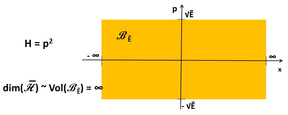
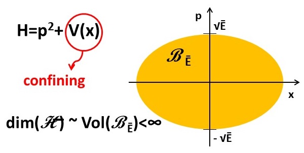
Figure 1: Classical phase space regions with energy $E\leq\overline{E}$

Technical details are given in sections 2, 3. Section 2 fixes the notation and contains preliminaries partly developed in [23]. The representation-theoretical results of section 3, which deserve attention also on their own, allow to explictly characterize the space $V_{D}^{l}$ as the space of harmonic homogeneous polynomials of degree $l$ in the Cartesian coordinates $x^{i}$ of $\mathbb{R}^{D}$ restricted to the sphere $S^{d}$; we determine such polynomials constructing the trace-free completely symmetric projector of $\left(\mathbb{R}^{D}\right)^{\otimes^{l}}$ and applying it to the homogeneous polynomials of degree $l$ in $x^{i}$. The actions of the $L_{hk}$ and of the multiplication operators $x^{i}\cdot$ on such polynomials can be expressed by general formulae valid for all $D,l$; this allows to avoid the rather complicated actions of the $L_{hk}$ on spherical harmonics (which also span $V_{D}^{l}$) used in [23]. It turns out that both ${\cal H}_{\Lambda},V_{D+1}^{\Lambda}$ decompose into irreps of $O(D)$ as follows:

$${\cal H}_{\Lambda}\simeq V_{D+1}^{\Lambda}=\bigoplus\limits_{l=0}^{\Lambda}V_{D}^{l},$$ (6)

The second equality shows that, in contrast with the mentioned fuzzy hyperspheres, we recover (2) in the limit $\Lambda\to\infty$. The first equality suggests that the unitary irrep of the $*$-algebra ${\cal A}_{\Lambda}$ on ${\cal H}_{\Lambda}$ is isomorphic to the irrep $\pi_{\Lambda}$ of $Uso(D+1)$ on $V_{D+1}^{\Lambda}$, what we in fact prove in section 5 (this had been proved for $D=2,3$ and conjectured for $D>3$ in [22, 23]). The relations fulfilled by $\overline{x}^{i},\overline{L}_{hk}$ are determined in section 4: the commutators $[\overline{x}^{i},\overline{x}^{j}]$ are also Snyder-like [1], i.e. are proportional to $\overline{L}_{hk}/k$, with a proportionality factor that is the same constant on all of ${\cal H}_{\Lambda}$, except on the $l=\Lambda$ component of the latter, where it is a slightly different constant. $\overline{x}^{i}$ generate the whole ${\cal A}_{\Lambda}$. The square distance $\overline{\bm{x}}^{2}\equiv\overline{x}^{i}\overline{x}_{i}$ is a function of ${\bm{L}}^{2}$ only, such that almost all its spectrum is very close to 1 and goes to 1 in the limit $\Lambda\to\infty$. In section 6 we show in which sense ${\cal H}_{\Lambda},{\cal A}_{\Lambda}$ go to ${\cal H},{\cal A}$ as $\Lambda\to\infty$, in particular how one can recover $f\cdot\in C(S^{d})\subset{\cal A}$, the multiplication operator of wavefunctions in ${\cal L}^{2}(S^{d})$ by a continuous function $f$, as the strong limit of a suitable sequence $f_{\Lambda}\in{\cal A}_{\Lambda}$ (again, this had been only conjectured in [23]). In section 7 we discuss our results and possible developments in comparison with the literature; in particular, we point out that our pair $({\cal H}_{\Lambda},{\cal A}_{\Lambda})$ can be seen as a fuzzy quantization of a coadjoint orbit of $O(D)$ that can be identified with the cotangent space $T^{*}S^{d}$, the classical phase space over the $d$-dimensional sphere. Finally, we have concentrated most proofs in the appendix 8.

2 General setting

We choose a set of real Cartesian coordinates $x:=(x^{1},...x^{D})$ of $\mathbb{R}^{D}$ and abbreviate $\partial_{i}\equiv\partial/\partial x^{i}$. We normalize $x^{i},\partial_{i}$ and $H$ itself so as to be dimensionless. Then we can express $r^{2}:={\bm{x}}^{2}\equiv x_{i}x^{i}$, $\Delta:=\partial_{i}\partial^{i}$ (sum over repeated indices understood), where actually $x_{i}=x^{i}$ and $\partial^{i}=\partial_{i}$ because the coordinates are real and Cartesian. The self-adjoint operators $x^{i},-i\partial_{i}$ on ${\cal L}^{2}(\mathbb{R}^{D})$ fulfill the canonical commutation relations

$$[x^{i},x^{j}]=0,\qquad[-i\partial_{i},-i\partial_{j}]=0,\qquad[x^{i},-i\partial_{j}]=i\delta^{i}_{j},$$ (7)

which are equivariant under all orthogonal transformations $Q$ (including parity $Q=-I$)

$$x^{i}\mapsto x^{\prime}{}^{i}=Q^{i}_{j}x^{j},\qquad Q^{-1}=Q^{T}.$$ (8)

All scalars $S$, in particular $S=\Delta,r^{2},V,H$, are invariant. This implies $[S,L_{ij}]=0$, where

$$L_{ij}:=i(x^{j}\partial_{i}-x^{i}\partial_{j})$$ (9)

are the angular momentum components associated to $x$. These generate rotations of $\mathbb{R}^{D}$, i.e.

$$[iL_{ij},v^{h}]=v^{i}\delta^{h}_{j}-v^{j}\delta^{h}_{i}$$ (10)

hold for the components $v^{h}$ of all vector operators, in particular $v^{h}=x^{h},\partial_{h}$, and close the commutation relations of $so(D)$,

$$[iL_{ij},iL_{hk}]=i\left(L_{ik}\delta_{hj}-L_{jk}\delta_{hi}-L_{ih}\delta_{kj}+L_{jh}\delta_{ki}\right).$$ (11)

The $D$ derivatives $\partial_{i}$ make up a globally defined basis for the linear space of smooth vector fields on $\mathbb{R}^{D}$. As the $L_{ij}$ are vector fields tangent to all spheres $r\!=$const, the set $B=\{\partial_{r},L_{ij}\>|\>i<j\}$ ($\partial_{r}:=\partial/\partial r$) is an alternative complete set that is singular for $r=0$, but globally defined elsewhere; for $D=2$ it is a basis, while for $D>2$ it is redundant, because of the relations

$$\varepsilon^{i_{1}i_{2}i_{3}....i_{D}}x^{i_{1}}L_{i_{2}i_{3}}=0.$$ (12)

This redundancy (unavoidable if $S^{d}$ is not parallelizable) will be no problem for our purposes.

We shall assume that $V(r)$ has a very sharp minimum at  $r=1$ with very large $k=V^{\prime\prime}(1)/4>0$,  and fix $V_{0}:=V(1)$ so that the ground state ${\bm{\psi}}_{0}$ has zero energy, i.e. $E_{0}=0$ (see fig. 3). We choose an energy cutoff $\overline{E}$ fulfilling first of all the condition

$$V(r)\simeq V_{0}+2k(r-1)^{2}\qquad\mbox{if $r$ fulfills}\quad V(r)\leq\overline{E},$$ (13)

so that we can neglect terms of order higher than two in the Taylor expansion of $V(r)$ around $1$ and approximate the potential as a harmonic one in the classical region $v_{\overline{E}}\subset\mathbb{R}^{D}$ determined by the condition  $V(r)\leq\overline{E}$.  By (13), $v_{\overline{E}}$ is approximately the spherical shell $|r\!-\!1|\leq\sqrt{\frac{\overline{E}\!-\!V_{0}}{2k}}$; when both $\overline{E}\!-\!V_{0}$ and $k$ diverge, while their ratio goes to zero, then $v_{\overline{E}}$ reduces to the unit sphere $S^{d}$. We expect that in this limit the dimension of ${\cal H}_{\overline{E}}$ diverges, and we recover standard quantum mechanics on $S^{d}$. As we shall see, this is the case.

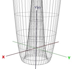
Figure 2: Three-dimensional plot of $V(r)$
in dimension $D=2$.

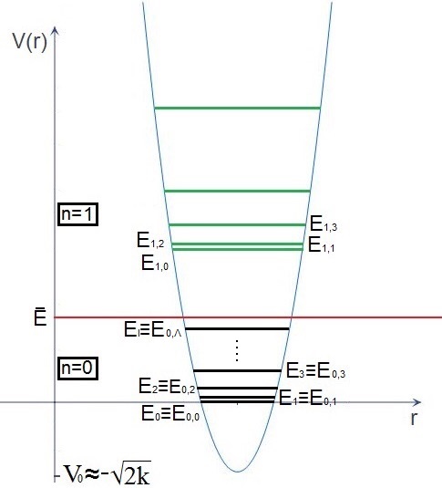
Figure 3: Two-dimensional plot of $V(r)$,
including the energy-cutoff.

Of course, the eigenfunctions of $H$ can be more easily determined in terms of polar coordinates $r,\theta_{1},...,\theta_{d}$, recalling that the Laplacian in $D$ dimensions decomposes as follows

$$\Delta=\partial_{r}^{2}+(D-1)\frac{1}{r}\partial_{r}-\frac{1}{r^{2}}{\bm{L}}^{2},$$ (14)

(see section 3.1) where ${\bm{L}}^{2}:=L_{ij}L_{ij}/2$ is the square angular momentum (in normalized units), i.e. the quadratic Casimir of $Uso(D)$ and the Laplacian on the sphere $S^{d}$; ${\bm{L}}^{2}$ can be expressed in terms of angles $\theta_{a}$ and derivatives $\partial/\partial\theta^{a}$ only. The eigenvalues of ${\bm{L}}^{2}$ are $l\left(l+D-2\right)$, see section 3.1; we denote by $V_{D}^{l}$ the ${\bm{L}}^{2}=E_{l}$ eigenspace within ${\cal L}^{2}(S^{d})$. Replacing the Ansatz  ${\bm{\psi}}=f(r)Y_{l}({\bm{\theta}})$,  with $f(r)=r^{-d/2}\,g(r)$, $Y_{l}\in V_{D}^{l}$, ${\bm{\theta}}\equiv(\theta_{1},...,\theta_{d})$,  transforms the Schrödinger PDE  $H{\bm{\psi}}=E{\bm{\psi}}$  into the Fuchsian ODE in the unknown $g(r)$

$$-g^{\prime\prime}(r)+\left[\frac{\left[D^{2}-4D+3+4l(l+D-2)\right]}{4r^{2}}+V(r)\right]g(r)=Eg(r).$$ (15)

The requirement ${\bm{\psi}}\in{\cal L}^{2}(\mathbb{R}^{D})$ implies that $g$ belongs to ${\cal L}^{2}(\mathbb{R}^{+})$, in particular goes to zero as $r\rightarrow\infty$. The self-adjointness of $H$ implies that it must be $f(0)=0$; this is compatible [23] with Fuchs theorem provided $r^{2}V(r)\overset{r\rightarrow 0^{+}}{\longrightarrow}T\in\mathbb{R}^{+}$ [what is in turn compatible with (13)]. Since $V(r)$ is very large outside the thin spherical shell $v_{\overline{E}}$ (a neighbourhood of $S^{d}$), $g,f,{\bm{\psi}}$ become negligibly small there, and, by condition (13), the lowest eigenvalues $E$ are at leading order those of the $1$-dimensional harmonic oscillator approximation [23] of (15)

$$-g^{\prime\prime}(r)+g(r)k_{l}\left(r-\widetilde{r}_{l}\right)^{2}=\widetilde{E}_{l}g(r),$$ (16)

which is obtained neglecting terms $O\big{(}(r\!-\!1)^{3}\big{)}$ in the Taylor expansions of $1/r^{2},V(r)$ about $r\!=\!1$. Here

$$\begin{array}[]{l}\widetilde{r}_{l}:=1+\frac{b(l,D)}{3b(l,D)+2k},\quad\widetilde{E}_{l}:=E-V_{0}\frac{2b(l,D)\left[k+b(l,D)\right]}{3b(l,D)+2k},\\[6.0pt] k_{l}:=2k+3b(l,D),\quad b(l,D):=\frac{D^{2}-4D+3+4l(l+D-2)}{4}.\end{array}$$ (17)

The (Hermite functions) square-integrable solutions of (16)

$$g_{n,l}(r)=M_{n,l}\hskip 4.26773pte^{-\frac{\sqrt{k_{l}}}{2}\left(r-\widetilde{r}_{l}\right)^{2}}\cdot H_{n}\left((r-\widetilde{r}_{l})\sqrt[4]{k_{l}}\right)\quad\mbox{ with }n\in\mathbb{N}_{0}$$

(here $M_{n,l}$ are normalization constants and $H_{n}$ are the Hermite polynomials) lead to

$$f_{n,l}(r)=\frac{M_{n,l}}{r^{\frac{d}{2}}}\hskip 4.26773pte^{-\frac{\sqrt{k_{l}}}{2}\left(r-\widetilde{r}_{l}\right)^{2}}\cdot H_{n}\left((r-\widetilde{r}_{l})\sqrt[4]{k_{l}}\right)\quad\mbox{ with }n\in\mathbb{N}_{0}.$$ (18)

The corresponding ‘eigenvalues’ in (16) $\widetilde{E}_{n,l}=(2n+1)\sqrt{k_{l}}$ lead to energies

$$E_{n,l}=(2n+1)\sqrt{k_{l}}+V_{0}+\frac{2b(l,D)[k+b(l,D)]}{3b(l,D)+2k}.$$

As said, we fix $V_{0}$ requiring that the lowest one $E_{0,0}$ be zero; this implies

$$V_{0}=-\sqrt{k_{0}}-\frac{2b(0,D)\left[k+b(0,D)\right]}{3b(0,D)+2k}=-\sqrt{2k}-b(0,D)-\frac{3b(0,D)}{2\sqrt{2k}}+O\left(k^{-\frac{1}{2}}\right),$$

and the expansions of $E_{n,l}$ and $\widetilde{r}_{l}$ at leading order in $k$ become

$$E_{n,l}=l(l+D-2)+2n\sqrt{2k}+O\left(k^{-\frac{1}{2}}\right),\qquad\widetilde{r}_{l}=1+\frac{b(l,D)}{2k}+O\left(k^{-2}\right).$$ (19)

$E_{0,l}$ coincide at lowest order with the desired eigenvalues $E_{l}$ of the Laplacian ${\bm{L}}^{2}$ on $S^{d}$, while if $n>0$ $E_{n,l}$ diverge as $k\to\infty$; to exclude all states with $n>0$ (i.e., to ‘freeze’ radial oscillations; then all corresponding classical trajectories are circles) we impose the cutoff

$$E_{n,l}\leq\overline{E}(\Lambda):=\Lambda(\Lambda\!+\!D\!-\!2)<2\sqrt{2k},\qquad\Lambda\in\mathbb{N}.$$ (20)

The right inequality is satisfied prescribing a suitable dependence $k\left(\Lambda\right)$, e.g. $k\left(\Lambda\right)=\left[\Lambda(\Lambda\!+\!D\!-\!2)\right]^{2}$; the left one is satisfied setting $n=0$ and $l\leq\Lambda$. Abbreviating $f_{l}\equiv f_{0,l}$, we end up with eigenfunctions and associated energies (at leading order in $1/\Lambda$)

$${\bm{\psi}}_{l}(r,{\bm{\theta}})=f_{l}(r)\,Y_{l}({\bm{\theta}}),\qquad H{\bm{\psi}}_{l}=E_{l}\,{\bm{\psi}}_{l},\qquad\quad l=0,1,...,\Lambda.$$ (21)

Thus ${\cal H}_{\Lambda}$ decomposes into irreps of $O(D)$ (and eigenspaces of ${\bm{L}}^{2},H$) as follows

$${\cal H}_{\Lambda}=\bigoplus_{l=0}^{\Lambda}{\cal H}_{\Lambda}^{l},\qquad{\cal H}_{\Lambda}^{l}:=f_{l}(r)\,V_{D}^{l}.$$ (22)

We can express the projectors $P^{l}_{\Lambda}:{\cal H}_{\Lambda}\to{\cal H}_{\Lambda}^{l}$ as the following polynomials in $\overline{{\bm{L}}}^{2}$:

$$P^{l}_{\Lambda}=\prod_{n=0,n\neq l}^{\Lambda}\frac{\overline{{\bm{L}}}^{2}-E_{n}}{E_{l}-E_{n}}.$$ (23)

In the commutative limit $\Lambda\to\infty$ the spectrum $\{E_{0,l}\}_{l=0}^{\Lambda}$ of $\overline{H}$ goes to the whole spectrum $\{E_{l}\}_{l\in\mathbb{N}_{0}}$ of $\bm{L}^{2}$. If ${\bm{\phi}},{\bm{\phi}}^{\prime}\in{\cal H}\equiv{\cal L}^{2}(\mathbb{R}^{D})$ can be factorized into radial parts $f(r),f^{\prime}(r)$ and angular parts $T,T^{\prime}\in\mathcal{L}^{2}(S^{d})$, i.e. ${\bm{\phi}}=f\,T$, ${\bm{\phi}}^{\prime}=f^{\prime}\,T^{\prime}$, then so can be their scalar product:

$$\left({\bm{\phi}},{\bm{\phi}}^{\prime}\right):=\int_{\mathbb{R}^{D}}d^{D}x\,{\bm{\phi}}^{*}(x){\bm{\phi}}^{\prime}(x)=\langle T,T^{\prime}\rangle\>\int^{\infty}_{0}\!\!\!dr\,r^{d}\,f^{*}(r)\,f^{\prime}(r).$$ (24)

Here we have denoted by $\langle\cdot,\cdot\rangle$ the scalar product of $\mathcal{L}^{2}(S^{d})$,

$$\langle T,T^{\prime}\rangle:=\int_{S^{d}}\!\!\!d\alpha\>T^{*}\,T^{\prime},$$ (25)

where $d\alpha$ is the $O(D)$-invariant measure on $S^{d}$. Assume that  ${\cal B}:=\{Y_{l}^{\bm{m}}\}_{(l,\bm{m})\in{\sf I}}$,  is an orthonormal basis of $\mathcal{L}^{2}(S^{d})$  consisting of eigenvectors of ${\bm{L}}^{2}$ (e.g. spherical harmonics),

$$\bm{L}^{2}\,Y_{l}^{\bm{m}}\,=\,E_{l}\>Y_{l}^{\bm{m}},\qquad\langle Y_{l^{\prime}}^{\bm{m^{\prime}}},Y_{l}^{\bm{m}}\rangle=\delta^{\bm{m}\bm{m^{\prime}}}\,\delta_{ll^{\prime}};$$ (26)

here $\bm{m}\!\in\!{\sf I}_{l}$ is a (multi-)index labelling the elements of an orthonormal basis  ${\cal B}_{l}\equiv\{Y_{l}^{\bm{m}}\}_{{\bm{m}}\in{\sf I}_{l}}$   of $V_{D}^{l}$, and ${\sf I}:=\left\{(l,\bm{m})\>|\>l\in\mathbb{N}_{0},\,\bm{m}\in{\sf I}_{l}\right\}$.  Then, by appropriate choices of the normalization constants of (18), one obtains as orthonormal bases respectively of ${\cal H}$ and ${\cal H}_{\Lambda}^{l}$

$${\cal B}^{\prime}:=\left\{{\bm{\psi}}_{n,l}^{\bm{m}}:=f_{n,l}(r)Y_{l}^{\bm{m}},\>\>|\>\>n\in\mathbb{N}_{0},\>\bm{l}\in{\cal I}\right\},\qquad{\cal B}_{l}^{\prime}:=\{{\bm{\psi}}_{0,l}^{\bm{m}}=f_{l}(r)\,Y_{l}^{\bm{m}}\}_{{\bm{m}}\in{\sf I}_{l}}.$$

The projector $\widetilde{P}_{\Lambda}^{l}:{\cal H}\to{\cal H}_{\Lambda}^{l}$ acts by

$$\left(\widetilde{P}_{\Lambda}^{l}{\bm{\phi}}\right)(x)=\sum_{\bm{m}\in{\sf I}_{l}}{\bm{\psi}}_{0,l}^{\bm{m}}(x)\>\left({\bm{\psi}}_{0,l}^{\bm{m}},\bm{\phi}\right)=\sum_{\bm{m}\in{\sf I}_{l}}{\bm{\psi}}_{0,l}^{\bm{m}}(x)\int_{\mathbb{R}^{D}}\!\!d^{D}x^{\prime}{\bm{\psi}}_{0,l}^{\bm{m}*}(x^{\prime})\bm{\phi}(x^{\prime}).$$

If ${\bm{\phi}}$ has the form  $\bm{\phi}(r,{\bm{\theta}})=\Theta_{j}({\bm{\theta}})\phi(r)$, with $\Theta_{j}\in V_{D}^{j}$,  then by (24), (26) this simplifies to

$$\left(\widetilde{P}_{\Lambda}^{l}\bm{\phi}\right)(r,{\bm{\theta}})=\delta_{lj}\,\Theta_{j}({\bm{\theta}})\,f_{l}(r)\int^{\infty}_{0}\!\!\!\!r^{d}dr\,f_{l}^{*}(r)\phi(r),$$ (27)

which is zero if $l\neq j$, has the same angular dependence $\Theta_{j}({\bm{\theta}})$ as $\bm{\phi}$ if $l=j$.

In next section we provide an explicit characterization of elements $\Theta_{l}\in V_{D}^{l}$ as polynomials in the coordinates $t^{i}$ of points of the unit sphere $S^{d}$, which fulfill the relation

$$t^{i}t_{i}=1\qquad\mbox{(sum over $i$)},$$ (28)

rather than as combinations of spherical harmonics $Y_{l}^{\bm{m}}({\bm{\theta}})$, $\bm{m}\in{\sf I}_{l}$.

3 Representations of $O(D)$ via polynomials in $x^{i}$, $t^{i}$

The differential operator ${\bm{L}}^{2}$ can be expressed as

$${\bm{L}}^{2}=\eta(D\!-\!2\!+\!\eta)-r^{2}\Delta,\qquad\eta:=x^{i}\partial_{i}.$$ (29)

The ‘dilatation operator’  $\eta$   and the Laplacian $\Delta$ fulfill

$$\eta x^{i}=x^{i}(\eta+1),\qquad \eta\partial_{i}=\partial_{i}(\eta-1),$$ (30)

$$\Delta x^{i}=x^{i}\Delta+2\partial^{i},\qquad \Delta r^{2}=r^{2}\Delta+4\eta+2D.$$ (31)

In particular, the action of $\eta$ on monomials in the $x^{i}$ amounts to multiplication by their total degree. In terms of polar coordinates it is  $\eta=r\partial_{r}$,  which replaced in (29) gives (14).

Let $\mathbb{C}[x^{1},...,x^{D}]$ be the space of complex polynomial functions on $\mathbb{R}^{D}$ and, for all $l\!\in\!\mathbb{N}_{0}$, let $W_{D}^{l}$ be the subspace of homogeneous ones of degree $l$. The monomials of degree $l$ $x^{i_{1}}x^{i_{2}}...x^{i_{l}}\in W_{D}^{l}$ can be reordered in the form $(x^{1})^{l_{1}}...(x^{D})^{l_{D}}$ and make up a basis of $W_{D}^{l}$:

$${\cal B}_{W_{D}^{l}}:=\left\{(x^{1})^{l_{1}}...(x^{D})^{l_{D}}\>|\>(l_{1},...,l_{D})\in\mathbb{N}_{0},\>\sum_{i=1}^{D}l_{i}=l\right\},\qquad\mbox{dim}(W_{D}^{l})={D\!+\!l\!-\!1\choose l};$$

the dimension of $W_{D}^{l}$ is the number of elements of ${\cal B}_{W_{D}^{l}}$. Clearly $W_{D}^{l}$ carries a representation of $O(D)$ as well as $Uso(D)$, but this is reducible if $l\geq 2$; in fact, the subspace $r^{2}W_{D}^{l-2}\subset W_{D}^{l}$ manifestly carries a smaller representation. We denote by $\check{V}_{D}^{l}$ the “trace-free” component of $W_{D}^{l}$, namely the subspace such that  $W_{D}^{l}=\check{V}_{D}^{l}\oplus r^{2}W_{D}^{l-2}$.  As a consequence,

$$\mbox{dim}(\check{V}_{D}^{l})=\mbox{dim}(W_{D}^{l})-\mbox{dim}(W_{D}^{l-2})=\frac{(l\!+\!D\!-\!3)...(l\!+\!1)}{(D\!-\!2)!}(D\!+\!2l\!-\!2).$$ (32)

$\check{V}_{D}^{l}$ carries the irreducible representation (irrep) ${\bm{\pi}}_{D}^{l}$ of $Uso(D)$ and $O(D)$ characterized by the highest eigenvalue of ${\bm{L}}^{2}$ within $W_{D}^{l}$, namely $E_{l}$ (the eigenvalues of all other $[D/2\!-\!1]$ Casimirs are determined by $l$). Abbreviating  $X_{l,\pm}^{hk}:=(x^{h}\!\pm\!ix^{k})^{l}$,  this can be easily shown observing that for all $h,k\in\{1,...,D\}$ $X_{l,\pm}^{hk}\in W_{D}^{l}$ are annihilated by $\Delta$ and are eigenvectors of ${\bm{L}}^{2}$ with that eigenvalue; moreover, they are eigenvectors of $L_{hk}$ with eigenvalue $\pm l$. Hence  $X_{l,+}^{hk}$, $X_{l,-}^{hk}$  can be used as the highest and lowest weight vectors of $\check{V}_{D}^{l}$. Since all the $L_{ij}$ commute with $\Delta$, $\check{V}_{D}^{l}$ can be characterized also as the subspace of $W_{D}^{l}$ which is annihilated by $\Delta$. A complete set in $\check{V}_{D}^{l}$ consists of trace-free homogeneous polynomials $X_{l}^{i_{1}i_{2}...i_{l}}$, which we will obtain below applying the completely symmetric trace-free projector ${\cal P}^{l}$ to the $x^{i_{1}}x^{i_{2}}...x^{i_{l}}$’s.

We slightly enlarge $\mathbb{C}[x^{1},...x^{D}]$ introducing as new generators $r,r^{-1}$ subject to the relations  $r^{2}=x^{i}x_{i}$ (sum over $i$), $rr^{-1}=1$. Inside this enlarged algebra the elements

$$t^{i}:=\frac{x^{i}}{r}$$ (37)

fulfill the relation (28) characterizing the coordinates of points of the unit sphere $S^{d}$. Choosing $g(r)=r^{-l}$ in (33-36) we obtain the same relations with  $x^{i},\,X_{l,\pm}^{hk}$ replaced by $t^{i},\,T_{l,\pm}^{hk}:=(t^{h}\!\pm\!it^{k})^{l}$.  We shall denote by $Pol_{D}$ the algebra of complex polynomials in such $t^{i}$, by $Pol_{D}^{\Lambda}$ the subspace of polynomials up to degree $\Lambda$, by $P^{\Lambda}:Pol_{D}\to Pol_{D}^{\Lambda}$ the corresponding projector. $Pol_{D}$ endowed with the scalar product  $\langle T,T^{\prime}\rangle:=\int_{S^{d}}d\alpha\,T^{*}T^{\prime}$  is a pre-Hilbert space; its completion is ${\cal L}^{2}(S^{d})$. We extend $P^{\Lambda}$ to all of ${\cal L}^{2}(S^{d})$ by continuity in the norm of the latter. Also $Pol_{D}^{\Lambda},V_{D}^{l}$ are Hilbert subspaces of ${\cal L}^{2}(S^{d})$. $Pol_{D}^{\Lambda}=W_{D}^{\Lambda}r^{-\Lambda}\oplus W_{D}^{\Lambda-1}r^{1-\Lambda}$ carries a unitary reducible representation of $O(D)$ [and $Uso(D)$] which splits via  $Pol_{D}^{\Lambda}=\bigoplus_{l=0}^{\Lambda}V_{D}^{l}$  into irreps carried by $V_{D}^{l}:=\check{V}_{D}^{l}/r^{l}$. Its dimension is thus

$$\mbox{dim}\left(Pol_{D}^{\Lambda}\right) = \sum_{l=0}^{\Lambda}\mbox{dim}(\check{V}_{D}^{l})=\sum_{l=0}^{\Lambda}\mbox{dim}(W_{D}^{l})-\sum_{l=2}^{\Lambda}\mbox{dim}(W_{D}^{l-2})$$ (38)

$$= \mbox{dim}(W_{D}^{\Lambda})+\mbox{dim}\left(W_{D}^{\Lambda-1}\right)$$

$$= \frac{(D\!+\!\Lambda\!-\!1)...(\Lambda\!+\!1)}{(D\!-\!1)!}+\frac{(D\!+\!\Lambda\!-\!2)...\Lambda}{(D\!-\!1)!}$$

$$= \frac{(D\!+\!\Lambda\!-\!2)...(\Lambda\!+\!1)}{(D\!-\!1)!}\left(D\!+\!2\Lambda\!-\!1\right)=:N$$

$$\stackrel{{\scriptstyle(\ref{dimVDl})}}{{=}} \mbox{dim}\left(V_{D+1}^{\Lambda}\right).$$ (39)

This suggests that ${\cal H}_{\Lambda}\simeq Pol_{D}^{\Lambda}\simeq V_{D+1}^{\Lambda}$ as $Uso(D)$ (reducible) representations. We have proved the first isomorphism in section 2 and will prove the second in section 3.2.

3.1 $O(D)$-irreps via trace-free completely symmetric projectors

Let $(\pi,{\cal E})$ be the $D$-dimensional irreducible unitary representation of $Uso(D)$ and $O(D)$; the carrier space ${\cal E}$ is isomorphic to $V_{D}^{1}$. As a vector space ${\cal E}\simeq\mathbb{R}^{D}$; the set of coordinates $x:=(x^{1},...x^{D})\in\mathbb{R}^{D}$ can be seen as the set of components of an element of ${\cal E}$ with respect to (w.r.t.) an orthonormal basis. The permutator on  ${\cal E}^{\otimes^{2}}\equiv{\cal E}\otimes{\cal E}$  is defined via ${\sf P}(u\otimes v)=v\otimes u$ and linearly extended. In all bases it is represented by the $D^{2}\times D^{2}$ matrix   ${\sf P}^{hi}_{jk}=\delta^{h}_{k}\delta^{i}_{j}$. The symmetric and antisymmetric projectors ${\cal P}^{+},{\cal P}^{-}$ on ${\cal E}^{\otimes^{2}}$ are obtained as

$${\cal P}^{\pm}=\frac{1}{2}\left({\bf 1}_{D^{2}}\pm{\sf P}\right);$$ (40)

here and below we denote by ${\bf 1}_{D^{l}}$ the identity operator on ${\cal E}^{\otimes^{l}}$, which in all bases is represented by the $D^{l}\times D^{l}$ matrix ${\bf 1}_{D^{l}}{}^{h_{1}...h_{l}}_{i_{1}...i_{l}}:=\delta^{h_{1}}_{i_{1}}...\delta^{h_{l}}_{i_{l}}$. The antisymmetrized tensor product ${\cal P}^{-}{\cal E}^{\otimes^{2}}$ is an irrep under $O(D)$, while the symmetrized one ${\cal P}^{+}{\cal E}^{\otimes^{2}}$ contains two irreps: the 1-dim trace one and the trace-free symmetric one. The matrix representation of the 1-dim projector ${\cal P}^{t}$ on the former is

$${\cal P}^{t}{}_{kl}^{ij}=\frac{1}{D}g^{ij}g_{kl}$$ (41)

where the $D\times D$ metric matrix $g_{ij}$ (in the chosen basis) is a $so(D)$-isotropic symmetric tensor, and $g^{ij}g_{jh}=\delta^{i}_{h}$, whence $g^{ij}g_{ij}=D$. Here we shall use an orthonormal basis of ${\cal E}$, whence $g_{ij}=g^{ij}=\delta_{ij}$, and indices of vector components can be raised or lowered freely, e.g. $x_{i}=x^{i}$. The $\frac{1}{2}(D\!-\!1)(D\!+\!2)$-dim trace-free symmetric projector ${\cal P}^{s}$ is given by

$${\cal P}^{s}:={\cal P}^{+}-{\cal P}^{t}=\frac{1}{2}\left({\bf 1}_{D^{2}}+{\sf P}\right)-{\cal P}^{t}\>.$$ (42)

These projectors satisfy the equations

$${\cal P}^{\alpha}{\cal P}^{\beta}={\cal P}^{\alpha}\delta^{\alpha\beta},\qquad\sum_{\alpha}{\cal P}^{\alpha}={\bf 1}_{D^{2}},$$ (43)

where $\alpha,\beta=-,s,t$. In the sequel we shall abbreviate ${\cal P}\equiv{\cal P}^{s}$. This implies in particular  ${\cal P}{\cal P}^{{}^{\prime}}=0$,  where we have introduced the new projector  ${\cal P}^{{}^{\prime}}:={\cal P}^{-}+{\cal P}^{t}$.  ${\sf P},{\cal P}^{t}$ are symmetric matrices, i.e. invariant under transposition ^T, and therefore also the other projectors are:

$${\sf P}^{T}={\sf P},\qquad\qquad{\cal P}^{\alpha}{}^{T}={\cal P}^{\alpha}.$$ (44)

Given a (linear) operator $M$ on ${\cal E}^{\otimes^{n}}$, for all integers $l,h$ with $l>n$, and $1\leq h\leq l\!+\!1\!-\!n$ we denote by $M_{h(h\!+\!1)...(h\!+\!n\!-\!1)}$ the operator on ${\cal E}^{\otimes^{l}}$ acting as the identity on the first $h\!-\!1$ and the last $l\!+\!1\!-\!n\!-\!h$ tensor factors, and as $M$ in the remaining central ones. For instance, if $M={\sf P}$ and $l=3$ we have ${\sf P}_{12}={\sf P}\otimes{\bf 1}_{D}$, ${\sf P}_{23}={\bf 1}_{D}\otimes{\sf P}$. It is straightforward to check

Proposition 3.1

All the projectors $A={\cal P}^{+},{\cal P}^{-},{\cal P},{\cal P}^{t},{\cal P}^{{}^{\prime}}$ fulfill the “braid” relation

$$A_{12}\,{\sf P}_{23}\,{\sf P}_{12}={\sf P}_{23}\,{\sf P}_{12}\,A_{23}.$$ (45)

Moreover,

$$D\>{\cal P}^{t}_{23}{\cal P}^{t}_{12}={\sf P}_{12}{\sf P}_{23}{\cal P}^{t}_{12},\quad\qquad D{\sf P}_{12}{\cal P}^{t}_{23}{\cal P}^{t}_{12}={\sf P}_{23}{\cal P}^{t}_{12},$$ (46)

$$D\>{\cal P}^{t}_{12}{\cal P}^{t}_{23}={\sf P}_{23}{\sf P}_{12}{\cal P}^{t}_{23},\quad\qquad D\>{\sf P}_{23}{\cal P}^{t}_{12}{\cal P}^{t}_{23}={\sf P}_{12}{\cal P}^{t}_{23,}$$ (47)

$$D\>{\cal P}^{t}_{23}{\cal P}^{t}_{12}={\cal P}^{t}_{23}{\sf P}_{12}{\sf P}_{23},\quad\qquad D\>{\cal P}^{t}_{23}{\cal P}^{t}_{12}{\sf P}_{23}={\cal P}^{t}_{23}{\sf P}_{12};$$ (48)

Eq. (45-48) hold also for $l>3$, e.g. for all $2\leq h\leq l-1$

$$A_{(h-1)h}\,{\sf P}_{h(h+1)}\,{\sf P}_{(h-1)h}={\sf P}_{h(h+1)}\,{\sf P}_{(h-1)h}\,A_{h(h+1)}.$$ (49)

Proof    Since $A={\bf 1}_{D^{2}},{\sf P},{\cal P}^{t}$ fulfill (45), then also $A={\cal P}^{+},{\cal P}^{-},{\cal P},{\cal P}^{t},{\cal P}^{{}^{\prime}}$ do. One can immediately check the first equality in (8.9) via direct calculation; left multiplying the first by ${\sf P}_{12}$ one obtains the second. Eq. (47) are obtained from (8.9) exchanging $1\leftrightarrow 3$ and using the symmetry of ${\sf P},{\cal P}^{t}$ under the flip. Eq. (48) are obtained from (47) by transposition. $\sqcap$$\sqcup$

Next, we define and determine the completely symmetric trace-free projector ${\cal P}^{l}$ on ${\cal E}^{\otimes^{l}}$ generalizing ${\cal P}^{2}\equiv{\cal P}$ to $l>2$. It projects the tensor product of $l$ copies of ${\cal E}$ to the carrier space of the $l$-fold completely symmetric irrep of $Uso(D)$, isomorphic to $V^{l}_{D}$, therein contained. It is uniquely characterized by the following properties:

$$\begin{array}[]{l}{\cal P}^{l}{\cal P}^{-}_{n(n\!+\!1)}=0,\quad{\cal P}^{l}{\cal P}^{t}_{n(n\!+\!1)}=0,\\[8.0pt] {\cal P}^{-}_{n(n\!+\!1)}{\cal P}^{l}=0,\quad{\cal P}^{t}_{n(n\!+\!1)}{\cal P}^{l}=0,\end{array}\qquad\qquad n=1,...,l\!-\!1$$ (52)

$$\left({\cal P}^{l}\right)^{2}={\cal P}^{l},$$ (53)

Consequently, it is also  $\mbox{tr}_{1\ldots l}\!\left({\cal P}^{l}\right)=\mbox{dim}(V^{l}_{D})$, which guarantees that ${\cal P}^{l}$ acts as the identity (and not as a proper projector) on $V^{l}_{D}$.  The right relations in (52) amount to

$${\cal P}^{l}{}^{i_{1}...i_{l}}_{j_{1}...j_{l}}\delta^{j_{n}j_{n+1}}=0,\quad\delta_{i_{n}i_{n+1}}{\cal P}^{l}{}^{i_{1}...i_{l}}_{j_{1}...j_{l}}=0,\qquad\qquad n=1,...,l\!-\!1.$$ (54)

Clearly the whole of (52) can be summarized as ${\cal P}^{l}{\cal P}^{{}^{\prime}}_{n(n\!+\!1)}=0={\cal P}^{{}^{\prime}}_{n(n\!+\!1)}{\cal P}^{l}$. It is straightforward to prove that the above properties imply also the ones

$${\cal P}^{l}{\sf P}_{n(n\!+\!1)}={\cal P}^{l},\quad n=1,...,l\!-\!1;\qquad{\cal P}^{l}{\cal P}^{h}_{(i+1)...(i+h)}={\cal P}^{l},\quad h<l,\>\>0\leq i\leq l\!-\!h.$$ (55)

Proposition 3.2

The projector ${\cal P}^{l\!+\!1}$ can be expressed as a polynomial in the permutators ${\sf P}_{12},...,{\sf P}_{(l\!-\!1)l}$ and trace projectors ${\cal P}^{t}_{12},...,{\cal P}^{t}_{(l\!-\!1)l}$ through either recursive relation

$${\cal P}^{l\!+\!1} = {\cal P}^{l}_{12...l}M_{l(l\!+\!1)}{\cal P}^{l}_{12...l},$$ (56)

$$= {\cal P}^{l}_{2...(l\!+\!1)}M_{12}{\cal P}^{l}_{2...(l\!+\!1)},$$ (57)

$$\mbox{where }\quad M\equiv M(l\!+\!1)=\frac{1}{l\!+\!1}\!\left[{\bf 1}_{D^{2}}+l\,{\sf P}-\frac{2Dl}{D\!+\!2l\!-\!2}{\cal P}^{t}\right]$$ (58)

As a consequence, the ${\cal P}^{l}$ are symmetric, $({\cal P}^{l})^{T}={\cal P}^{l}$.

This the analog of Proposition 1 in [26] for the quantum group $U_{q}so(D)$ covariant symmetric projectors; the proof is in the appendix. By a straightforward computation one checks that

$${\cal P}^{l+1}{}^{hi_{1}...i_{l}}_{hj_{1}...j_{l}}=\frac{1}{l\!+\!1}\!\left[D+l-\frac{2l}{D\!+\!2l\!-\!2}\right]{\cal P}^{l}{}^{i_{1}...i_{l}}_{j_{1}...j_{l}}$$ (59)

($h$ is summed over). Using (31), (54) one easily shows that the homogeneous polynomials

$$X_{l}^{i_{1}...i_{l}}:={\cal P}^{l}{}^{i_{1}...i_{l}}_{j_{1}...j_{l}}x^{j_{1}}...x^{j_{l}}\in\check{V}^{l}_{D}$$ (60)

are harmonic, i.e. satisfy $\Delta X_{l}^{i_{1}...i_{l}}=0$; using (29), we find that they are eigenvectors of ${\bm{L}}^{2}$,

$${\bm{L}}^{2}\,X_{l}^{i_{1}...i_{l}}=\,E_{l}\,X_{l}^{i_{1}...i_{l}},$$ (61)

with eigenvalues (3). They make up a complete set in $\check{V}_{D}^{l}$, which can be thus also characterized as the subspace of $W_{D}^{l}$ that is annihilated by $\Delta$, whereas $\Delta\phi\neq 0$ for all $\phi\in r^{2}W_{D}^{l-2}$. The $X_{l}^{i_{1}...i_{l}}$ are not all independent, because they are invariant under permutations of $(i_{1}...i_{l})$ and by (54) fulfill the linear dependence relations

$$\delta_{i_{n}i_{n+1}}X_{l}^{i_{1}...i_{l}}=0,\qquad\qquad n=1,...,l\!-\!1.$$ (62)

Proposition 3.3

In a compact notation,

$$\begin{array}[]{l}\left({\cal P}^{l}_{1...l}-{\cal P}^{l+1}\right)x_{1}...x_{l+1}=\zeta_{l+1}\,{\cal P}^{l}_{1...l}{\cal P}^{t}_{l(l\!+\!1)}x_{1}...x_{l+1},\\[8.0pt] \left({\cal P}^{l}_{2...(l\!+\!1)}-{\cal P}^{l+1}\right)x_{1}...x_{l+1}=\zeta_{l+1}\,{\cal P}^{l}_{2...(l\!+\!1)}{\cal P}^{t}_{12}x_{1}...x_{l+1},\end{array}\qquad\zeta_{l+1}=\frac{D\,l}{D\!+\!2l\!-\!2}.$$ (65)

The proof is in Appendix 8.2. More explicitly, (65) becomes

$$x^{h}X_{l}^{i_{1}...i_{l}}-X_{l+1}^{hi_{1}...i_{l}}=\frac{\zeta_{l+1}}{D}r^{2}\,{\cal P}^{l}{}^{i_{1}i_{2}...i_{l}}_{hj_{2}...j_{l}}x^{j_{2}}...x^{j_{l}}=\frac{\zeta_{l+1}}{D}r^{2}\,{\cal P}^{l}{}^{i_{1}i_{2}...i_{l}}_{hj_{2}...j_{l}}X_{l-1}^{j_{2}...j_{l}}$$ (66)

Contracting the previous relation with $\delta_{hi_{1}}$ and using (54) we obtain

$$x^{h}X_{l}^{hi_{2}...i_{l}}=\frac{\zeta_{l+1}}{D}r^{2}\,{\cal P}^{l}{}^{hi_{2}...i_{l}}_{hj_{2}...j_{l}}X_{l-1}^{j_{2}...j_{l}}\stackrel{{\scriptstyle(\ref{contractPs})}}{{=}}\frac{r^{2}}{D\!+\!2l\!-\!2}\left[D\!+\!l\!-\!1\!-\!\frac{2l\!-\!2}{D\!+\!2l\!-\!4}\right]X_{l-1}^{i_{2}...i_{l}}.$$ (67)

In the Appendix we also prove

Proposition 3.4

The maps $L_{hk}:\check{V}_{D}^{l}\to\check{V}_{D}^{l}$ explicitly act as follows:

$$\begin{array}[]{lll}iL_{hk}X_{l}^{i_{1}...i_{l}}&=&\displaystyle l\,\frac{\zeta_{l+2}}{\zeta_{l+1}}\left({\cal P}^{l+1}{}^{hi_{1}...i_{l}}_{kj_{1}...j_{l}}-{\cal P}^{l+1}{}^{ki_{1}...i_{l}}_{hj_{1}...j_{l}}\right)X_{l}^{j_{1}...j_{l}},\\[8.0pt] &=&\displaystyle l\,{\cal P}^{l}{}^{i_{1}...i_{l}}_{j_{1}...j_{l}}\left(\delta^{kj_{1}}X_{l}^{hj_{2}...j_{l}}-\delta^{hj_{1}}X_{l}^{kj_{2}...j_{l}}\right).\end{array}$$ (70)

Dividing (61), (62), (66), (67), (70) by the appropriate powers of $r$ we find

Proposition 3.5

The  $T_{l}^{i_{1}i_{2}...i_{l}}:=X_{l}^{i_{1}i_{2}...i_{l}}/r^{l}={\cal P}^{l}{}^{i_{1}...i_{l}}_{j_{1}...j_{l}}t^{j_{1}}...t^{j_{l}}$  belong to $V_{D}^{l}$, because

$${\bm{L}}^{2}\,T_{l}^{i_{1}...i_{l}} = E_{l}\,T_{l}^{i_{1}...i_{l}};$$ (71)

they make up a complete set ${\cal T}_{l}$ in it, but not a basis, because they are invariant under permutations of $(i_{1}...i_{l})$ and by (62) fulfill the linear dependence relations

$$\delta_{i_{n}i_{n+1}}T_{l}^{i_{1}...i_{l}}=0,\qquad\qquad n=1,...,l\!-\!1.$$ (72)

The actions of the operators  $t^{h}\cdot$, $iL_{hk}$ on the $T_{l}^{i_{1}...i_{l}}$ explicitly read

$$t^{h}\,T_{l}^{i_{1}...i_{l}}=T_{l+1}^{hi_{1}...i_{l}}+\frac{l}{D\!+\!2l\!-\!2}\,{\cal P}^{l}{}^{i_{1}i_{2}...i_{l}}_{hj_{2}...j_{l}}T_{l-1}^{j_{2}...j_{l}}\>\in\>V_{D}^{l+1}\oplus V_{D}^{l-1},$$ (73)

$$t^{i}T_{l}^{ii_{2}...i_{l}}=\frac{1}{D\!+\!2l\!-\!2}\left[D\!+\!l\!-\!1\!-\!\frac{2l\!-\!2}{D\!+\!2l\!-\!4}\right]T_{l-1}^{i_{2}...i_{l}}\>\in\>V_{D}^{l-1},$$ (74)

$$\begin{array}[]{lll}iL_{hk}T_{l}^{i_{1}...i_{l}}&=&\displaystyle l\,\frac{\zeta_{l+2}}{\zeta_{l+1}}\left({\cal P}^{l+1}{}^{hi_{1}...i_{l}}_{kj_{1}...j_{l}}-{\cal P}^{l+1}{}^{ki_{1}...i_{l}}_{hj_{1}...j_{l}}\right)T_{l}^{j_{1}...j_{l}},\\[8.0pt] &=&\displaystyle l\,{\cal P}^{l}{}^{i_{1}...i_{l}}_{j_{1}...j_{l}}\left(\delta^{kj_{1}}T_{l}^{hj_{2}...j_{l}}-\delta^{hj_{1}}T_{l}^{kj_{2}...j_{l}}\right).\end{array}$$ (77)

For all ${\bm{\phi}}\in{\cal H}_{s}\equiv{\cal L}^{2}(S^{d})$ let

$${\bm{\phi}}=\sum_{l=0}^{\infty}\sum_{\bm{m}\in{\sf I}_{l}}\phi^{l}_{\bm{m}}Y_{l}^{\bm{m}}=\sum_{l=0}^{\infty}\sum_{i_{1},....,i_{l}}\phi^{l}_{i_{1}...i_{l}}T_{l}^{i_{1}...i_{l}}$$ (78)

be its decompositions in the basis of spherical harmonics and in the complete set ${\cal T}:=\bigcup_{l=0}^{\infty}{\cal T}_{l}$; here the two sets of coefficients are related by $\phi^{l}_{i_{1}...i_{l}}=\sum_{\bm{m}\in{\sf I}_{l}}\phi^{l}_{\bm{m}}A^{\bm{m}}_{i_{1}...i_{l}}$, where $A^{\bm{m}}_{i_{1}...i_{l}}$ are such that $Y_{l}^{\bm{m}}=\sum A^{\bm{m}}_{i_{1}...i_{l}}T_{l}^{i_{1}...i_{l}}$. The $\phi^{l}_{i_{1}...i_{l}}$ are uniquely determined if, as we shall assume, we choose them trace-free and completely symmetric, i.e. fulfilling

$$\phi^{l}_{i_{1}...i_{l}}=\phi^{l}_{j_{1}...j_{l}}\,{\cal P}^{l}{}_{i_{1}...i_{l}}^{j_{1}...j_{l}},$$ (79)

whence $\phi^{l}_{i_{1}...i_{l}}\delta^{i_{n}i_{n+1}}=0$ for $n=1,...,l\!-\!1$. Then (78) can be also written in the form

$${\bm{\phi}}=\sum_{l=0}^{\infty}\sum_{i_{1},....,i_{l}}\phi^{l}_{i_{1}...i_{l}}t^{i_{1}}...\,t^{i_{l}}.$$ (80)

The projector $P_{\Lambda}$ acts by truncation,  $P_{\Lambda}{\bm{\phi}}\equiv{\bm{\phi}}_{\Lambda}:=\sum_{l=0}^{\Lambda}\sum_{\bm{m}\in{\sf I}_{l}}\phi^{l}_{\bm{m}}Y_{l}^{\bm{m}}=\sum_{l=0}^{\Lambda}\phi^{l}_{i_{1}...i_{l}}T_{l}^{i_{1}...i_{l}}$ (sum over $i_{1},....,i_{l}$). Clearly $\phi_{\Lambda}\stackrel{{\scriptstyle\Lambda\to\infty}}{{\longrightarrow}}\phi$ in the ${\cal H}_{s}$-norm $\|\,\|$.

All completely symmetric, $O(D)$-isotropic tensors of even rank ${\overline{N}}$ are proportional to

$$G_{\overline{N}}^{i_{1}...i_{\overline{N}}}:=\delta^{i_{1}i_{2}}\delta^{i_{3}i_{4}}...\delta^{i_{{\overline{N}}-1}i_{\overline{N}}}\,+\mbox{permutations of }\>(i_{1},...,i_{\overline{N}}).$$ (81)

Proposition 3.6

The ‘trace’ of $G_{\overline{N}}$,  $\mbox{tr}\left(G_{\overline{N}}\right):=\delta_{i_{1}i_{2}}\delta_{i_{3}i_{4}}...\delta_{i_{{\overline{N}}-1}i_{\overline{N}}}G_{\overline{N}}^{i_{1}...i_{\overline{N}}}$,  is equal to

$$\mbox{tr}\left(G_{\overline{N}}\right)=\overline{N}!!\,D(D\!+\!2)...(D\!+\!{\overline{N}}\!-\!2).$$ (82)

The $O(D)$-invariant integral over $S^{d}$ of the tensor $H_{\overline{N}}^{i_{1}...i_{\overline{N}}}:=t^{i_{1}}...t^{i_{\overline{N}}}$ is equal to

$$\int_{S^{d}}d\alpha\>t^{i_{1}}...t^{i_{\overline{N}}}=C_{\overline{N}}\,G_{\overline{N}}^{i_{1}...i_{\overline{N}}},\qquad C_{\overline{N}}=\frac{\mbox{mis}(S^{d})}{\overline{N}!!\,D(D\!+\!2)...(D\!+\!{\overline{N}}\!-\!2)}.$$ (83)

In terms of the decompostions (78b)-(79) the scalar product of generic ${\bm{\phi}},{\bm{\psi}}\subset{\cal H}_{s}$ is equal to

$$\langle{\bm{\phi}},{\bm{\psi}}\rangle=\sum_{l=0}^{\infty}Q_{l}\big{(}\phi^{l}_{i_{1}...i_{l}}\big{)}^{*}\psi^{l}_{i_{1}...i_{l}},\qquad Q_{l}:=C_{2l}\,2^{l}(l!)^{2}=\frac{\mbox{mis}(S^{d})\,l!\,(D\!-\!2)!!}{(D\!+\!2l\!-\!2)!!}.$$ (84)

In particular, (84) implies  $\left\langle T_{l}^{i_{1}...i_{l}},T_{n}^{j_{1}...j_{n}}\right\rangle=\delta_{ln}Q_{l}\,{\cal P}^{l}{}_{i_{1}...i_{l}}^{j_{1}...j_{l}}$  and more generally

$$\left\langle T_{l}^{i_{1}...i_{l}},{\bm{\phi}}\right\rangle=Q_{l}\,{\cal P}^{l}{}_{i_{1}...i_{l}}^{j_{1}...j_{l}}\phi^{l}_{j_{1}...j_{l}}\stackrel{{\scriptstyle(\ref{phi-coeff-prop})}}{{=}}Q_{l}\,\phi^{l}_{i_{1}...i_{l}},$$ (85)

the second equality holds only if (79) holds. Then, we have also

$$\|{\bm{\phi}}\|^{2}\equiv\langle{\bm{\phi}},{\bm{\phi}}\rangle=\sum_{l=0}^{\infty}Q_{l}\sum_{i_{1},...,i_{l}}\!\!\big{|}\phi^{l}_{i_{1}...i_{l}}\big{|}^{2}.$$ (86)

We now determine the decomposition of $T_{l}^{i_{1}...i_{l}}T_{m}^{j_{1}...j_{m}}$.

Theorem 3.7

The product $T_{l}^{i_{1}...i_{l}}T_{m}^{j_{1}...j_{m}}$ decomposes as follows into $V_{D}^{n}$ components:

$$T_{l}^{i_{1}...i_{l}}T_{m}^{j_{1}...j_{m}}=\sum\limits_{n\in L^{lm}}\,S^{i_{1}...i_{l},j_{1}...j_{m}}_{k_{1}...k_{n}}T_{n}^{k_{1}...k_{n}},$$ (87)

where $L^{lm}:=\{|l\!-\!m|,|l\!-\!m|\!+\!2,...,l\!+\!m\}$ and, defining  $\displaystyle r\!:=\!\frac{l\!+\!m\!-\!n}{2}\in\{0,1,...,m\}$,

$$\begin{array}[]{l}\displaystyle S^{i_{1}...i_{l},j_{1}...j_{m}}_{k_{1}...k_{n}}=N^{lm}_{n}\,V^{i_{1}...i_{l},j_{1}...j_{m}}_{k_{1}...k_{n}},\qquad N^{lm}_{n}=\frac{(D\!+\!2n\!-\!2)!!\,l!\,m!}{(D\!+\!2n\!+\!2r\!-\!2)!!\,(l\!-\!r)!\,(m\!-\!r)!}\\[10.0pt] V^{i_{1}...i_{l},j_{1}...j_{m}}_{k_{1}...k_{n}}={\cal P}^{l}{}_{a_{1}...a_{r}c_{1}...c_{l-r}}^{i_{1}...i_{l}}{\cal P}^{m}{}_{a_{1}...a_{r}c_{l-r+1}...c_{n}}^{j_{1}...j_{r}j_{r+1}...j_{m}}{\cal P}^{n}{}_{c_{1}...c_{n}}^{k_{1}...k_{n}}.\end{array}$$ (90)

The coefficients $S^{i_{1}...i_{l},j_{1}...j_{m}}_{k_{1}...k_{n}}$ are the analogs of the Clebsch-Gordon coefficients, which appear in the decomposition of a product of two spherical harmonics into a combination of spherical harmonics for $D=3$. The first term of the sum (87) is  $T_{l+m}^{i_{1}...i_{l}j_{1}...j_{m}}$. This is consistent with the first term in the iterated application of (73). If $r\!=\!m\!=\!1$, since ${\cal P}^{1}{}_{a_{1}}^{j_{1}}=\delta^{j_{1}}_{a_{1}}$, $n=l\!-\!1$, the result is consistent with the second term in (73):

$$S^{i_{1}...i_{l},j_{1}}_{k_{1}...k_{l\!-\!1}}=\frac{l}{D\!+\!2l\!-\!2}\,{\cal P}^{l}{}_{j_{1}k_{1}...k_{l-1}}^{i_{1}...i_{l}}.$$

3.2 Embedding in $\mathbb{R}^{D+1}$, isomorphism $\mbox{End}\!\left(Pol_{D}^{\Lambda}\right)\simeq{\bf\pi}_{D+1}^{\Lambda}\big{[}Uso(D\!+\!1)\big{]}$

We naturally embed $\mathbb{C}[\mathbb{R}^{D}]\hookrightarrow\mathbb{C}[\mathbb{R}^{\bf D}]$, where ${\bf D}\equiv D+1$. Henceforth we use real Cartesian coordinates $(x^{i})$ for $\mathbb{R}^{D}$ and $(x^{I})$ for $\mathbb{R}^{\bf D}$; $h,i,j,k\in\{1,...,D\}$, $H,I,J,K\in\{1,...,{\bf D}\}$. We naturally embed $O(D)\hookrightarrow SO({\bf D})$ identifying $O(D)$ as the subgroup of $SO({\bf D})$ which is the little group of the ${\bf D}$-th axis; its Lie algebra, isomorphic to $so(D)$, is generated by the $L_{hk}$. We shall add ${\bf D}$ as a subscript to distinguish objects in this enlarged dimension from their counterparts in dimension $D$, e.g. the distance $r_{\bf D}$ from the origin in $\mathbb{R}^{\bf D}$, from its counterpart $r\equiv r_{D}$ in $\mathbb{R}^{D}$, ${\cal P}^{l}_{\bf D}$ from ${\cal P}^{l}\equiv{\cal P}^{l}_{D}$, and so on.

We look for the decomposition of each $\check{V}_{\bf D}^{\Lambda}$ into irreps of such a $Uso(D)$. Clearly, $\check{V}_{\bf D}^{0}\simeq\mathbb{C}\simeq V_{D}^{0}$, while $\check{V}_{\bf D}^{1}=\check{V}_{D,1}^{0}\oplus\check{V}_{D,1}^{1}$, where $\check{V}_{D,1}^{0}\simeq V_{D}^{0}$ is spanned by $x^{\bf D}$, and $\check{V}_{D,1}^{1}\simeq V_{D}^{1}$ is spanned by the $x^{i}$. The $X_{{\bf D},2}^{IJ}=x^{I}x^{J}-r_{\bf D}^{2}\delta^{IJ}/{\bf D}$ span $\check{V}_{\bf D}^{2}$; the set of elements

$$X_{{\bf D},2}^{{\bf D}{\bf D}}=x^{\bf D}x^{\bf D}-\frac{r_{\bf D}^{2}}{{\bf D}},\qquad X_{{\bf D},2}^{i{\bf D}}=x^{i}x^{\bf D},\qquad X_{2}^{ij}=X_{{\bf D},2}^{ij}+\frac{\delta^{ij}}{D}X_{{\bf D},2}^{{\bf D}{\bf D}}$$ (91)

span carrier spaces $\check{V}_{D,2}^{0},\check{V}_{D,2}^{1},\check{V}_{D,2}^{2}$ respectively isomorphic to $V_{D}^{0},V_{D}^{1},V_{D}^{2}$, and  $\check{V}_{\bf D}^{2}=\check{V}_{D,2}^{2}\oplus\check{V}_{D,2}^{1}\oplus\check{V}_{D,2}^{0}$.  More generally, $\check{V}_{\bf D}^{\Lambda}$ is spanned by the the $X_{{\bf D},\Lambda}^{I_{1}...I_{\Lambda}}$, which are homogeneous polynomials of degree $\Lambda$ in the $x^{I}$ obtained by (60) in dimension ${\bf D}$, i.e.

$$X_{{\bf D},l}^{I_{1}...I_{l}}:={\cal P}_{\bf D}^{l}{}^{I_{1}...I_{l}}_{J_{1}...J_{l}}x^{J_{1}}...x^{J_{l}}\in\check{V}^{l}_{\bf D}$$ (92)

where the projectors ${\cal P}_{\bf D}^{l}$ are constructed as in Proposition 3.2, but with $D$ replaced by ${\bf D}$. Any pair of indices $I_{a},I_{b}$ appears either through the product $x^{I_{a}}x^{I_{b}}$ or through $r_{\bf D}^{2}\delta^{I_{a}I_{b}}$. If we introduce $r_{\bf D}$ as a further generator constrained by the relation $r_{\bf D}^{2}=x^{I}x^{I}$ (sum over $I$), then the $X_{{\bf D},\Lambda}^{I_{1}...I_{\Lambda}}$ can be seen also as homogeneous polynomials of degree $\Lambda$ in $x^{I},r_{\bf D}$.  Since $\delta^{j_{a}{\bf D}}=0$, in $X_{{\bf D},\Lambda}^{j_{1}...j_{l}{\bf D}...{\bf D}}$: any pair of indices ${\bf D}{\bf D}$ appears either through the product $x^{{\bf D}}x^{{\bf D}}$ or through $r_{\bf D}^{2}\delta^{{\bf D}{\bf D}}=r_{\bf D}^{2}$; any pair of indices $j_{a},{\bf D}$ appears through the product $x^{j_{a}}x^{I_{b}}$; any pair of indices $j_{a},j_{b}$ appears either through the product $x^{j_{a}}x^{j_{b}}$ or through $r_{\bf D}^{2}\delta^{j_{a}j_{b}}$. By property (54), the latter terms completely disappear in any combination ${\cal P}^{l}{}^{i_{1}...i_{l}}_{j_{1}...j_{l}}X_{{\bf D},\Lambda}^{j_{1}...j_{l}{\bf D}...{\bf D}}$, $l\in\{2,3,...,\Lambda\}$.  Therefore such a combination can be factorized as follows

$$\check{F}^{i_{1}...i_{l}}_{{\bf D},\Lambda}\>:=\>{\cal P}^{l}{}^{i_{1}...i_{l}}_{j_{1}...j_{l}}X_{{\bf D},\Lambda}^{j_{1}...j_{l}{\bf D}...{\bf D}}\>=\>\check{p}_{\Lambda,l}\,X_{l}^{i_{1}...i_{l}},$$ (93)

where $\check{p}_{\Lambda,l}$ is a homogeneous polynomial of degree $\Lambda-l$ in $x^{\bf D},r_{\bf D}$ of the form

$$\check{p}_{\Lambda,l}=\left(x^{\bf D}\right)^{\Lambda-l}+\left(x^{\bf D}\right)^{\Lambda-l-2}r_{\bf D}^{2}\,b_{\Lambda,l+2}+\left(x^{\bf D}\right)^{\Lambda-l-4}r_{\bf D}^{4}\,b_{\Lambda,l+4}+...\>\>;$$ (94)

the coefficients $b_{\Lambda,h}$ can be determined from $\Delta_{\bf D}\,\check{F}^{i_{1}...i_{l}}_{{\bf D},\Lambda}\!=\!0$, which follows from $\Delta_{\bf D}\,X_{{\bf D},\Lambda}^{I_{1}...I_{\Lambda}}\!=\!0$.

Proposition 3.8

$\check{V}_{\bf D}^{\Lambda}$ decomposes into the following irreducible components of $Uso(D)$:

$$\check{V}_{\bf D}^{\Lambda}=\bigoplus_{l=0}^{\Lambda}\check{V}_{D,\Lambda}^{l},$$ (95)

where $\check{V}_{D,\Lambda}^{l}\simeq V_{D}^{l}$ is spanned by the $\check{F}^{i_{1}...i_{l}}_{{\bf D},\Lambda}$, since the latter are eigenvectors of ${\bm{L}}^{2}$:

$${\bm{L}}^{2}\check{F}^{i_{1}...i_{l}}_{{\bf D},\Lambda}=E_{l}\check{F}^{i_{1}...i_{l}}_{{\bf D},\Lambda}.$$ (96)

Denoting by $[a]$ the integral part of $a\in\mathbb{R}^{+}$, the coefficients of (94) are given by

$$b_{\Lambda,l+2k}=(-)^{k}\frac{(\Lambda\!-\!l)!\,(2\Lambda\!-\!4\!-\!2k\!+\!{\bf D})!!}{(\Lambda\!-\!l\!-\!2k)!\,(2k)!!\,(2\Lambda\!-\!4\!+\!{\bf D})!!},\qquad k=1,2,....\left[\frac{\Lambda\!-\!l}{2}\right].$$ (97)

The $\check{F}^{i_{1}...i_{l}}_{{\bf D},\Lambda}$ transform under $L_{hk}$ as the $T^{i_{1}...i_{l}}_{l}$, and under $L_{h{\bf D}}$ as follows:

$$iL_{h{\bf D}}\check{F}^{i_{1}...i_{l}}_{{\bf D},\Lambda}=(\Lambda\!-\!l)\,\check{F}_{{\bf D},\Lambda}^{hi_{1}...i_{l}}-\frac{l(\Lambda\!+\!l\!+\!D\!-\!2)}{D\!+\!2l\!-\!2}\>{\cal P}^{l}{}^{i_{1}i_{2}...i_{l}}_{hj_{2}...j_{l}}\,\check{F}_{{\bf D},\Lambda}^{j_{2}...j_{l}}\,.$$ (98)

The proof is in Appendix 8.5. We now determine the decomposition of $V_{\bf D}^{\Lambda}:=\check{V}_{\bf D}^{\Lambda}/(r_{\bf D})^{\Lambda}$ into irreps of $Uso(D)$. $V_{\bf D}^{0}\simeq V_{D}^{0}\simeq\mathbb{C}$ is spanned by 1.  $V_{\bf D}^{1}=V_{D,1}^{0}\oplus V_{D,1}^{1}$, where $V_{D,1}^{0}\simeq V_{D}^{0}$ is spanned by $t^{\bf D}$, and $V_{D,1}^{1}\simeq V_{D}^{1}$ is spanned by the $t^{i}$ (here $t^{I}:=x^{I}/r_{\bf D}$). $V_{\bf D}^{2}$ is spanned by the $T_{{\bf D},2}^{IJ}=t^{I}t^{J}\!-\!\frac{\delta^{IJ}}{{\bf D}}$; more explicitly,

$$T_{{\bf D},2}^{{\bf D}{\bf D}}=t^{\bf D}t^{\bf D}-\frac{1}{{\bf D}}=\frac{D}{{\bf D}}-t^{h}t_{h},\qquad T_{{\bf D},2}^{i{\bf D}}=t^{i}t^{\bf D},\qquad T_{{\bf D},2}^{ij}=t^{i}t^{j}-\delta^{ij}\frac{1}{{\bf D}};$$

$F_{{\bf D},2}:=T_{{\bf D},2}^{{\bf D}{\bf D}}$ spans an irrep $V_{D,2}^{0}$ isomorphic to $V_{D}^{0}$, the $F_{{\bf D},2}^{i}:=T_{{\bf D},2}^{i{\bf D}}$ span an irrep $V_{D,2}^{1}$ isomorphic to $V_{D}^{1}$, while the $F_{D,2}^{ij}:={\cal P}^{ij}_{hk}T_{{\bf D},2}^{hk}$ (which fulfill $F_{D,2}^{ij}\delta_{ij}=0$) span an irrep $V_{D,2}^{2}$ isomorphic $V_{D}^{2}$. The $F_{D,2}^{ij}$ can be expressed as combinations of the $T_{{\bf D},2}^{IJ}$:

$$F_{D,2}^{ij}=T_{{\bf D},2}^{ij}+\frac{\delta^{ij}}{D}T_{{\bf D},2}^{{\bf D}{\bf D}}=T_{{\bf D},2}^{ij}-\frac{\delta^{ij}}{D}T_{{\bf D},2}^{hh}\>(\mbox{sum over }h)=t^{i}t^{j}-\frac{\delta^{ij}}{D}t^{h}t_{h}$$

This shows the decomposition  $V_{\bf D}^{2}=V_{D,2}^{2}\oplus V_{D,2}^{1}\oplus V_{D,2}^{0}\simeq Pol_{D}^{2}$   explicitly. More generally, let

$$F^{i_{1}...i_{l}}_{{\bf D},\Lambda}:=\check{F}^{i_{1}...i_{l}}_{{\bf D},\Lambda}/(r_{\bf D})^{\Lambda}={\cal P}^{l}{}^{i_{1}...i_{l}}_{j_{1}...j_{l}}T_{{\bf D},\Lambda}^{j_{1}...j_{l}{\bf D}...{\bf D}}=p_{\Lambda,l}{\cal P}^{l}{}^{i_{1}...i_{l}}_{j_{1}...j_{l}}t^{j_{1}}...t^{j_{l}}=:p_{\Lambda,l}T_{l}^{i_{1}...i_{l}},$$ (99)

where we have introduced a polynomial $p_{\Lambda,l}$ of degree $h=\Lambda-l$ in $t^{\bf D}$ (containing only powers of the same parity as $h$) by $p_{\Lambda,l}:=\check{p}_{\Lambda,l}(x^{\bf D},r_{\bf D})\,r_{\bf D}^{l-\Lambda}$; more explicitly the latter reads

$$p_{\Lambda,l}=\left(t^{\bf D}\right)^{\Lambda-l}+\left(t^{\bf D}\right)^{\Lambda-l-2}b_{\Lambda,l+2}+\left(t^{\bf D}\right)^{\Lambda-l-4}b_{\Lambda,l+4}+...\>\>.$$ (100)

As a direct consequence of Propositions 3.8, dividing all relations by $(r_{\bf D})^{\Lambda}$, we find

Corollary 3.9

$V_{\bf D}^{\Lambda}$ decomposes into the following irreducible components of $Uso(D)$:

$$V_{\bf D}^{\Lambda}=\bigoplus_{l=0}^{\Lambda}V_{D,\Lambda}^{l},$$ (101)

where $V_{D,\Lambda}^{l}\simeq V_{D}^{l}$ is spanned by the $F^{i_{1}...i_{l}}_{{\bf D},\Lambda}$. The latter are eigenvectors of ${\bm{L}}^{2}$,

$${\bm{L}}^{2}F^{i_{1}...i_{l}}_{{\bf D},\Lambda}=E_{l}F^{i_{1}...i_{l}}_{{\bf D},\Lambda},$$ (102)

transform under $L_{hk}$ as the $T^{i_{1}...i_{l}}_{l}$, and under $L_{h{\bf D}}$ as follows:

$$iL_{h{\bf D}}F^{i_{1}...i_{l}}_{{\bf D},\Lambda}=(\Lambda\!-\!l)\,F_{{\bf D},\Lambda}^{hi_{1}...i_{l}}-\frac{l(\Lambda\!+\!l\!+\!D\!-\!2)}{D\!+\!2l\!-\!2}\>{\cal P}^{l}{}^{i_{1}i_{2}...i_{l}}_{hj_{2}...j_{l}}\,F_{{\bf D},\Lambda}^{j_{2}...j_{l}}\,.$$ (103)

For convenience, we slightly enlarge $Uso(D)$ by introducing the new generator

$$\lambda=\frac{1}{2}\left[\sqrt{(D\!-\!2)^{2}+4{\bm{L}}^{2}}-D+2\right],$$ (104)

which fulfills  $\lambda(\lambda\!+\!D\!-\!2)={\bm{L}}^{2}$,  so that $V_{D}^{l}$ is a $\lambda=l$ eigenspace, and  $\lambda\,F^{i_{1}...i_{l}}_{{\bf D},\Lambda}=l\,F^{i_{1}...i_{l}}_{{\bf D},\Lambda}$.

Proposition 3.10

There exist a $Uso(D)$-module isomorphism $\hat{\varkappa}_{\Lambda}:Pol_{D}^{\Lambda}\rightarrow V_{\bf D}^{\Lambda}$ and a $Uso(D)$-equivariant algebra isomorphism $\hat{\kappa}_{\Lambda}:\mbox{End}\!\left(Pol_{D}^{\Lambda}\right)\to{\bm{\pi}}_{\bf D}^{\Lambda}\big{[}Uso({\bf D})\big{]}$ such that

$$\hat{\varkappa}_{\Lambda}(aT)=\hat{\kappa}_{\Lambda}(a)\hat{\varkappa}_{\Lambda}(T),\qquad\forall\>T\in Pol_{D}^{\Lambda},\quad a\in\mbox{End}\!\left(Pol_{D}^{\Lambda}\right)\>.$$ (105)

On the $T_{l}^{i_{1}...i_{l}}$ (spanning $Pol_{D}^{\Lambda}$) and on generators $L_{hi},P^{\Lambda}t^{i}\cdot$ of $\mbox{End}\!\left(Pol_{D}^{\Lambda}\right)$ they act by

$$\hat{\varkappa}_{\Lambda}\left(T_{l}^{i_{1}...i_{l}}\right):=\hat{a}_{\Lambda,l}F^{i_{1}...i_{l}}_{{\bf D},\Lambda}=\hat{a}_{\Lambda,l}p_{\Lambda,l}T_{l}^{i_{1}...i_{l}},\qquad l=0,1,...,\Lambda,$$ (106)

$$\hat{\kappa}_{\Lambda}\left(L_{hi}\right):=L_{hi},\qquad\hat{\kappa}_{\Lambda}\left(P^{\Lambda}t^{i}\cdot\right):=\hat{m}_{\Lambda}^{*}(\lambda)L_{{\bf D}i}\hat{m}_{\Lambda}(\lambda),$$ (107)

where

$$\hat{m}_{\Lambda}(l)=\sqrt{\frac{\Gamma\!\left(\frac{\Lambda+l+D-1}{2}\right)\,\Gamma\!\left(\frac{\Lambda-l+1}{2}\right)}{2\,\Gamma\!\left(\frac{\Lambda+l+D}{2}\right)\,\Gamma\!\left(\frac{\Lambda-l}{2}+1\right)}},\quad\hat{a}_{\Lambda,l}=\hat{a}_{\Lambda,0}\,i^{l}\sqrt{\frac{\Lambda(\Lambda\!-\!1)...(\Lambda\!-\!l\!+\!1)}{(\Lambda\!+\!D\!-\!1)(\Lambda\!+\!D)...(\Lambda\!+\!l\!+\!D\!-\!2)}}.$$ (108)

The proposition and its proof are obtained from Theorem 5.1 and the associated proof by fixing $\Lambda$, taking $k$ independent of $\Lambda$ and letting the $k\to\infty$.

4 Relations among the $\overline{x}^{i},\overline{L}_{hk}$

Since for all fixed $l=0,1,...,\Lambda$ the $T_{l}^{i_{1}i_{2}...i_{l}}$, make up a complete set ${\cal T}_{l}$ in $V_{D}^{l}$, then the functions

$${\bm{\psi}}_{l}^{i_{1}i_{2}...i_{l}}:=T_{l}^{i_{1}i_{2}...i_{l}}f_{l}$$ (109)

($i_{h}\in\{1,...,D\}$ for $h\in\{1,...,l\}$) make up a complete set ${\cal S}^{l}_{D,\Lambda}$ in the eigenspace ${\cal H}_{\Lambda}^{l}$ of $H$, ${\bm{L}}^{2}$, with eigenvalues $E_{0,l}$, $E_{l}$. They are not linearly independent, because they are completely symmetric under permutation of the indices and fulfill the relations

$$\delta_{i_{n}i_{n+1}}{\bm{\psi}}_{l}^{i_{1}...i_{l}}=0,\qquad\qquad n=1,...,l\!-\!1.$$ (110)

${\cal S}_{D,\Lambda}:=\cup_{l=0}^{\Lambda}{\cal S}^{l}_{D,\Lambda}$ is a complete set in ${\cal H}_{\Lambda}$. By (109), (77) the $\overline{L}_{hk}$ act on the ${\bm{\psi}}_{l}^{i_{1}i_{2}...i_{l}}$ via

$$i\overline{L}_{hk}{\bm{\psi}}_{l}^{i_{1}i_{2}...i_{l}} = \displaystyle l\,{\cal P}^{l}{}^{i_{1}...i_{l}}_{j_{1}...j_{l}}\left(\delta^{kj_{1}}{\bm{\psi}}_{l}^{hj_{2}...j_{l}}-\delta^{hj_{1}}{\bm{\psi}}_{l}^{kj_{2}...j_{l}}\right).$$ (111)

By (27), (73), applying $P_{\Lambda}=\sum_{l=0}^{\Lambda}P^{l}_{\Lambda}$ to $x^{i}{\bm{\psi}}^{i_{1}i_{2}...i_{l}}=t^{i}\,T_{l}^{i_{1}i_{2}...i_{l}}\,rf_{l}(r)$ we find

$$P_{\Lambda}\left(x^{i}{\bm{\psi}}_{l}^{i_{1}i_{2}...i_{l}}\right) = c_{l+1}\,{\bm{\psi}}_{l+1}^{ii_{1}...i_{l}}+c_{l}\,\frac{\zeta_{l+1}}{D}\,{\cal P}^{l}{}^{i_{1}i_{2}...i_{l}}_{ij_{2}...j_{l}}{\bm{\psi}}_{l-1}^{j_{2}...j_{l}},$$

$$\mbox{where }\quad c_{l} := \left\{\!\!\begin{array}[]{ll}\sqrt{1+\frac{(2D\!-\!5)(D\!-1\!)}{2k}+\frac{(l\!-\!1)(l\!+\!D\!-\!2)}{k}}&\mbox{if }1\leq l\leq\Lambda,\\[6.0pt] 0&\mbox{otherwise,}\end{array}\right.\quad$$ (114)

up to order $O\left(k^{-3/2}\right)$, see appendix 8.6. Hence, at the same order,

$$\overline{x}^{i}{\bm{\psi}}_{l}^{i_{1}i_{2}...i_{l}}=c_{l+1}\,{\bm{\psi}}_{l+1}^{ii_{1}...i_{l}}+\frac{c_{l}\,l}{D\!+\!2l\!-\!2}\,{\cal P}^{l}{}^{i_{1}i_{2}...i_{l}}_{ij_{2}...j_{l}}\,{\bm{\psi}}_{l-1}^{j_{2}...j_{l}}.$$ (115)

The $O\left(k^{-3/2}\right)$ corrections depend on the terms proportional to $(r\!-\!1)^{k}$, $k>2$, in the Taylor expansion of $V$. These could be set rigorously equal to zero by a suitable choice of $V$. Henceforth we adopt (111-115) as exact definitions of $\overline{L}_{hk},\overline{x}^{i}$. In the appendix we prove

Proposition 4.1

The $\overline{x}^{i},\overline{L}_{hk}$ are self-adjoint operators generating the $N^{2}$-dimensional $*$-algebra  ${\cal A}_{\Lambda}:=End({\cal H}_{\Lambda})\simeq M_{N}(\mathbb{C})$  of observables on ${\cal H}_{\Lambda}$;   $N$ is given by (38). Abbreviating  $\overline{{\bm{x}}}^{2}:=\overline{x}^{i}\,\overline{x}^{i}$, $\overline{{\bm{L}}}^{2}:=\overline{L}_{ij}\,\overline{L}_{ij}/2$, $B:=(2D\!-\!5)(D\!-1\!)/2$,  they fulfill, at leading order in $1/\sqrt{k}$,

$$[i\overline{L}_{ij},\overline{x}^{h}]=\overline{x}^{i}\delta^{h}_{j}\!-\!\overline{x}^{j}\delta^{h}_{i},$$ (116)

$$[i\overline{L}_{ij},i\overline{L}_{hk}]=i\left(\overline{L}_{ik}\delta^{j}_{h}\!-\!\overline{L}_{jk}\delta^{i}_{h}\!-\!\overline{L}_{ih}\delta^{j}_{k}\!+\!\overline{L}_{jh}\delta^{i}_{k}\right),$$ (117)

$$\varepsilon^{i_{1}i_{2}i_{3}....i_{D}}\overline{x}^{i_{1}}\overline{L}_{i_{2}i_{3}}=0,\qquad D\geq 3,$$ (118)

$$(\overline{x}^{h}\!\pm\!i\overline{x}^{k})^{2\Lambda+1}=0,\quad(\bar{L}^{hj}\!+\!i\bar{L}^{kj})^{2\Lambda+1}=0,\qquad\mbox{if }h\neq j\neq k\neq h,$$ (119)

$$\left[\overline{x}^{i},\overline{x}^{j}\right]=i\overline{L}_{ij}\left(\!-\frac{I}{k}\!+\!K\,P_{\Lambda}^{\Lambda}\!\!\right),\quad\begin{array}[]{l}K:=\frac{1}{k}\!+\!\frac{1}{D\!+\!2\Lambda\!-\!2}\left[1\!+\!\frac{B}{k}\!+\!\frac{(\Lambda\!-\!1)(\Lambda\!+\!D\!-\!2)}{k}\right],\end{array}$$ (121)

$$\overline{{\bm{x}}}^{2}=1\!+\!\frac{\overline{{\bm{L}}}^{2}}{k}\!+\!\frac{B}{k}-\frac{\Lambda\!+\!D\!-\!2}{2\Lambda\!+\!D\!-\!2}\left[1\!+\!\frac{B}{k}\!+\!\frac{\Lambda(\Lambda\!+\!D\!-\!1)}{k}\right]P_{\Lambda}^{\Lambda}=:\chi({\bm{L}}^{2}).$$ (122)

This is the analog of Proposition 4.1 in [22]. We obtain a fuzzy sphere choosing $k$ as a function $k(\Lambda)$ fulfilling (20), e.g.  $k=\Lambda^{2}(\Lambda\!+\!D\!-\!2)^{2}/4$;  the commutative limit is  $\Lambda\rightarrow\infty$.

Remarks:

1. Eq. (118) is the analog of (12). By (121), it can be reformulated also in the form $\varepsilon^{i_{1}i_{2}i_{3}....i_{D}}\overline{x}^{i_{1}}\overline{x}^{i_{2}}\overline{x}^{i_{3}}=0$.

2. $\overline{{\bm{x}}}^{2}$ is not a constant, but by (122), (23)_l=Λ can be expressed as a polynomial $\chi$ in $\overline{{\bm{L}}}^{2}$ only, with the same eigenspaces ${\cal H}_{\Lambda}^{l}$. All its eigenvalues $r^{2}_{l}$, except $r^{2}_{\Lambda}$, are close to 1, slightly (but strictly) grow with $l$ and collapse to 1 as $\Lambda\to\infty$. Conversely, $\overline{{\bm{L}}}^{2}$ can be expressed as a polynomial $\upsilon$ in $\overline{{\bm{x}}}^{2}$, via  $\overline{{\bm{L}}}^{2}=\sum_{l=0}^{\Lambda}E_{l}P^{l}_{\Lambda}$ and $P^{l}_{\Lambda}=\prod_{n=0,n\neq l}^{\Lambda}\frac{\overline{{\bm{x}}}^{2}-r^{2}_{n}}{r^{2}_{l}-r^{2}_{n}}$.

3. By (121), (23)_l=Λ the commutators $[\overline{x}^{i},\overline{x}^{j}]$ are Snyder-like, i.e. of the form $\alpha\overline{L}_{ij}$; also $\alpha$ depends only on the $\overline{L}_{hk}$, more precisely can be expressed as a polynomial in $\overline{{\bm{L}}}^{2}$.

4. Using (116), (117), (121), all polynomials in $\overline{x}^{i},\overline{L}_{hk}$ can be expressed as combinations of monomials in $\overline{x}^{i},\overline{L}_{hk}$ in any prescribed order, e.g. in the natural one

   $$\left(\overline{x}^{1}\right)^{n_{1}}...\left(\overline{x}^{D}\right)^{n_{D}}\left(\overline{L}_{12}\right)^{n_{12}}\left(\overline{L}_{13}\right)^{n_{13}}...\left(\overline{L}_{dD}\right)^{n_{dD}},\qquad n_{i},n_{ij}\in\mathbb{N}_{0};$$ (123)

   the coefficients, which can be put at the right of these monomials, are complex combinations of 1 and $P^{\Lambda}_{\Lambda}$. Also $P^{\Lambda}_{\Lambda}$ can be expressed as a polynomial in $\overline{{\bm{L}}}^{2}$ via (23)_l=Λ. Hence a suitable subset (depending on $\Lambda$) of such ordered monomials makes up a basis of the $N^{2}$-dim vector space  ${\cal A}_{\Lambda}$.

5. Actually, $\overline{x}^{i}$ generate the $*$-algebra ${\cal A}_{\Lambda}$, because also the $\overline{L}_{ij}$ can be expressed as non-ordered polynomials in the $\overline{x}^{i}$: by (121) $\overline{L}_{ij}=[\overline{x}^{j},\overline{x}^{i}]/\alpha$, and also $1/\alpha$, which depends only on $P^{\Lambda}_{\Lambda}$, can be expressed itself as a polynomial in $\overline{{\bm{x}}}^{2}$, as shown above.

6. Eq. (116-122) are equivariant under the whole group $O(D)$, including the inversion $\overline{x}^{i}\!\mapsto\!-\overline{x}^{i}$ of one axis, or more (e.g. parity), contrary to Madore’s and Hoppe’s FS.

The operator norm of $\overline{{\bm{x}}}^{2}$ equals its highest eigenvalue,  $\|\overline{{\bm{x}}}^{2}\|_{op}=r^{2}_{\Lambda-1}=1\!+\![B\!+\!(\Lambda\!-\!1)(\Lambda\!+\!D\!-\!3)]/k$.  For all ${\bm{\psi}}\in{\cal H}_{\Lambda}$ and $i=1,...,D$, we find $\|\overline{x}^{i}{\bm{\psi}}\|^{2}=\langle\overline{x}^{i}{\bm{\psi}},\overline{x}^{i}{\bm{\psi}}\rangle\leq\sum_{i=1}^{D}\langle\overline{x}^{i}{\bm{\psi}},\overline{x}^{i}{\bm{\psi}}\rangle=\langle{\bm{\psi}},\overline{{\bm{x}}}^{2}{\bm{\psi}}\rangle\leq\|\overline{{\bm{x}}}^{2}\|_{op}\,\|{\bm{\psi}}\|^{2}$, whence

$$\|\overline{x}^{i}\|_{op}\leq\sqrt{1\!+\!\frac{B\!+\!(\Lambda\!-\!1)(\Lambda\!+\!D\!-\!3)}{k}}\leq 1\!+\!\epsilon,\quad\epsilon:=\frac{B\!+\!(\Lambda\!-\!1)(\Lambda\!+\!D\!-\!3)}{2k}$$ (124)

5 Isomorphisms of ${\cal H}_{\Lambda},{\cal A}_{\Lambda}$, and $*$-automorphisms of ${\cal A}_{\Lambda}$

Theorem 5.1

There exist a $O(D)$-module isomorphism $\varkappa_{\Lambda}:{\cal H}_{\Lambda}\rightarrow V_{\bf D}^{\Lambda}$ and a $O(D)$-equivariant algebra map $\kappa_{\Lambda}:{\cal A}_{\Lambda}\equiv\mbox{End}\!\left({\cal H}_{\Lambda}\right)\to{\bm{\pi}}_{\bf D}^{\Lambda}\big{[}Uso({\bf D})\big{]}$, ${\bf D}\equiv D\!+\!1$, such that

$$\varkappa_{\Lambda}(a{\bm{\psi}})=\kappa_{\Lambda}(a)\varkappa_{\Lambda}({\bm{\psi}}),\qquad\forall\>{\bm{\psi}}\in{\cal H}_{\Lambda},\quad a\in{\cal A}_{\Lambda}\>.$$ (125)

On the ${\bm{\psi}}_{l}^{i_{1}...i_{l}}$ (spanning ${\cal H}_{\Lambda}$) and on generators $L_{hi},\overline{x}^{i}\cdot$ of ${\cal A}_{\Lambda}$ they respectively act as follows:

$$\varkappa_{\Lambda}\left({\bm{\psi}}_{l}^{i_{1}...i_{l}}\right):=a_{\Lambda,l}F^{i_{1}...i_{l}}_{{\bf D},\Lambda}=a_{\Lambda,l}\,p_{\Lambda,l}\,T_{l}^{i_{1}...i_{l}},\qquad l=0,1,...,\Lambda,$$ (126)

$$\kappa_{\Lambda}\left(\overline{L}_{hi}\right):={\bm{\pi}}_{\bf D}^{\Lambda}(L_{hi})\,,\qquad\kappa_{\Lambda}\left(\overline{x}^{i}\right):={\bm{\pi}}_{\bf D}^{\Lambda}\big{[}m_{\Lambda}^{*}(\lambda)\,X^{i}\,m_{\Lambda}(\lambda)\big{]}\,,$$ (127)

where  $X^{i}:=L_{{\bf D}i}$,  $p_{\Lambda,l}=p_{\Lambda,l}\!\left(t^{\bf D}\right)$  are the polynomials (100), and

$$a_{\Lambda,l}=a_{\Lambda,0}\,i^{l}\sqrt{\frac{\Lambda(\Lambda\!-\!1)...(\Lambda\!-\!l\!+\!1)}{(\Lambda\!+\!D\!-\!1)(\Lambda\!+\!D)...(\Lambda\!+\!l\!+\!D\!-\!2)}},$$ (128)

$$m_{\Lambda}(s)=\sqrt{\frac{\Gamma\!\left(\frac{\Lambda+s+d}{2}\right)\,\Gamma\!\left(\frac{\Lambda-s+1}{2}\right)\,\Gamma\!\left(\frac{s+1+d/2+iA}{2}\right)\,\Gamma\!\left(\frac{s+1+d/2-iA}{2}\right)}{\Gamma\!\left(\frac{\Lambda+s+D}{2}\right)\,\Gamma\!\left(\frac{\Lambda-s}{2}+1\right)\,\Gamma\!\left(\frac{s+d/2+iA}{2}\right)\,\Gamma\!\left(\frac{s+d/2-iA}{2}\right)\,\sqrt{k}}};$$ (129)

here  $A:=\sqrt{k+(D\!-\!1)(D\!-\!3)3/4}$,  and $\Gamma$ is Euler gamma function.

The proof is in appendix 8.8.  The theorem extends Propositions 3.2, 4.2 of [22] to $d>2$. The claims for $d>2$ were partially formulated, but not proved, in [23].

As already recalled, the group of $*$-automorphisms of ${\cal A}_{\Lambda}\simeq M_{N}(\mathbb{C})$ is inner and isomorphic to $SU(N)$, i.e. of the type

$$a\mapsto g\,a\,g^{-1},\qquad a\in M_{N}(\mathbb{C}),$$ (130)

with $g$ an unitary $N\times N$ matrix with unit determinant. We can identify in $SU(N)$ a subgroup $\simeq SO({\bf D})$, acting via the $N$-dimensional representation $(V_{\bf D}^{\Lambda},{\bm{\pi}}_{\bf D}^{\Lambda})$; namely, it consists of matrices of the form $g={\bm{\pi}}_{\bf D}^{\Lambda}\left[e^{i\alpha}\right]$, where $\alpha\in so({\bf D})$. Choosing $\alpha\in so(D)\subset so({\bf D})$ the automorphism amounts to a $SO(D)\subset SO({\bf D})$ transformation, i.e. a rotation in the $x\equiv(x^{1},...,x^{D})\in\mathbb{R}^{D}$ space. $O(D)\subset SO({\bf D})$ transformations with determinant $-1$ in this space keep the same form in the $\overline{X}\equiv(X^{1},...,X^{D})$ space (where $X^{i}\equiv L_{{\bf D}i}$) and by (127) also in the $\overline{x}\equiv(\overline{x}^{1},...,\overline{x}^{D})$ space. In particular, those inverting one or more axes of $\mathbb{R}^{D}$ (i.e. changing the sign of one or more $x^{i}$, and thus also of $X^{i},\overline{x}^{i}$), e.g. parity, can be also realized as $SO({\bf D})$ transformations, i.e. rotations in $\mathbb{R}^{\bf D}$. This shows that (127) is equivariant under parity and the whole $O(D)$, which plays the role of isometry group of this fuzzy sphere.

6 Fuzzy spherical harmonics, and limit $\Lambda\to\infty$

In this section we suppress Einstein’s summation convention over repeated indices. The previous results allow to define $Uso(D)$-module Hilbert space isomorphisms

$$\begin{array}[]{lccccc}\sigma_{\Lambda}\>:&Pol_{D}^{\Lambda}\>=\>\displaystyle\bigoplus\limits_{l=0}^{\Lambda}&\>\>V_{D}^{l}&\to&{\cal H}_{\Lambda}\>=\>\displaystyle\bigoplus\limits_{l=0}^{\Lambda}&\>\>{\cal H}_{\Lambda}^{l},\\ &&\>\rotatebox[origin={c}]{90.0}{$\in$}&&&\>\rotatebox[origin={c}]{90.0}{$\in$}\\ &&T_{l}^{i_{1}...i_{l}},Y_{l}^{\bm{m}}&\mapsto&&{\bm{\psi}}_{l}^{i_{1}...i_{l}},{\bm{\psi}}_{l}^{\bm{m}};\end{array}$$ (134)

here ${\bm{\psi}}_{l}^{\bm{m}}:=\sum A^{\bm{m}}_{i_{1}...i_{l}}{\bm{\psi}}_{l}^{i_{1}...i_{l}}$. The objects at the right of the arrows are our fuzzy analogs of the objects at the left. In the limit $\Lambda\to\infty$ the above decomposition of ${\cal H}_{\Lambda}$ into irreducible components under $O(D)$ becomes isomorphic to the decomposition of $Pol_{D}\simeq{\cal H}_{s}$.

We define the $O(D)$-equivariant embedding   ${\cal I}:{\cal H}_{\Lambda}\hookrightarrow{\cal H}_{s}$   by setting   ${\cal I}\left({\bm{\psi}}_{l}^{i_{1}...i_{l}}\right):=T_{l}^{i_{1}...i_{l}}$  and applying linear extension. Below we drop ${\cal I}$ and identify ${\bm{\psi}}_{l}^{i_{1}...i_{l}}=T_{l}^{i_{1}...i_{l}}$, or equivalently ${\bm{\psi}}_{l}^{\bm{m}}=Y_{l}^{\bm{m}}$, as elements of the Hilbert space ${\cal H}_{s}$. For all ${\bm{\phi}}\equiv\sum_{l=0}^{\infty}\phi^{l}_{i_{1}...i_{l}}T_{l}^{i_{1}...i_{l}}\in{\cal L}^{2}(S^{2})$ and $\Lambda\in\mathbb{N}$ let ${\bm{\phi}}_{\Lambda}:=P_{\Lambda}{\bm{\phi}}=\sum_{l=0}^{\Lambda}\phi^{l}_{i_{1}...i_{l}}T_{l}^{i_{1}...i_{l}}$ be its projection to ${\cal H}_{\Lambda}$ (or $\Lambda$-th truncation). Clearly ${\bm{\phi}}_{\Lambda}\to{\bm{\phi}}$ in the ${\cal H}_{s}$-norm $\|\,\|$: in this simplified notation,  ${\cal H}_{\Lambda}$ ‘invades’ ${\cal H}_{s}$ as $\Lambda\to\infty$;

${\cal I}$ induces the $O(D)$-equivariant embedding of operator algebras  ${\cal J}\!:\!{\cal A}_{\Lambda}\!\hookrightarrow\!B\left({\cal H}_{s}\right)$  by setting ${\cal J}(a)\,{\cal I}({\bm{\psi}}):={\cal I}(a{\bm{\psi}})$;  here $B\left({\cal H}_{s}\right)$ stands for the $*$-algebra of bounded operators on ${\cal H}_{s}$. By construction ${\cal A}_{\Lambda}$ annihilates ${\cal H}_{\Lambda}^{\perp}$.  In particular, ${\cal J}\!\left(\overline{L}_{hk}\right)=L_{hk}P^{\Lambda}$, and $\overline{L}_{hk}{\bm{\phi}}\stackrel{{\scriptstyle\Lambda\to\infty}}{{\longrightarrow}}L_{hk}{\bm{\phi}}$  for all ${\bm{\phi}}\!\in\!D(L_{hk})\equiv$ the domain of $L_{hk}$. More generally, $f(\overline{L}_{hk})\to f(L_{hk})$ strongly on $D[f(L_{hk})]\subset{\cal H}_{s}$, for all measurable functions $f(s)$.

Continuous functions $f$ on $S^{d}$, acting as multiplication operators $f\cdot:{\bm{\phi}}\in{\cal H}_{s}\mapsto f{\bm{\phi}}\in{\cal H}_{s}$, make up a subalgebra $C(S^{d})$ of $B\left({\cal H}_{s}\right)$.  Clearly, $f$ belongs also to ${\cal H}_{s}$. Since $Pol_{D}$ is dense in both ${\cal H}_{s}$, $C(S^{d})$, $f_{N}$ converges to $f$ as $N\to\infty$ in both the ${\cal H}_{s}$ and the $C(S^{d})$ norm.

We define the $\Lambda$-th fuzzy analogs of the $T_{l}^{i_{1}...i_{l}}$ (seen as an element of $C(S^{d})$, i.e. acting by multiplication on ${\bm{\psi}}\in{\cal H}_{s}$), $l\leq\Lambda$, by replacing $t^{i}\cdot\mapsto\overline{x}^{i}$ in the definition of $T_{l}^{i_{1}...i_{l}}$, i.e. by

$$\widehat{T}_{l}^{i_{1}...i_{l}}:={\cal P}^{l}{}^{i_{1}...i_{l}}_{j_{1}...j_{l}}\overline{x}^{j_{1}}...\overline{x}^{j_{l}},$$ (135)

sum over repeated indices (cf. Proposition 3.5); the $\widehat{T}_{l}^{i_{1}...i_{l}}$ fulfill again (72). Having identified  ${\bm{\psi}}_{l}^{i_{1}...i_{l}}\equiv T_{l}^{i_{1}...i_{l}}$, we rewrite (73), (115) in the form

$$t^{h}\,T_{l}^{i_{1}...i_{l}}=T_{l+1}^{hi_{1}...i_{l}}+d_{l}\,{\cal P}^{l}{}^{i_{1}i_{2}...i_{l}}_{hj_{2}...j_{l}}T_{l-1}^{j_{2}...j_{l}},\qquad d_{l}:=\frac{l}{D\!+\!2l\!-\!2}$$ (136)

$$\overline{x}^{h}T_{l}^{i_{1}i_{2}...i_{l}}=c_{l+1}\,T_{l+1}^{hi_{1}...i_{l}}+c_{l}\>d_{l}\,{\cal P}^{l}{}^{i_{1}i_{2}...i_{l}}_{hj_{2}...j_{l}}\,T_{l-1}^{j_{2}...j_{l}}.$$ (137)

Using these formulae in appendix 8.9 we prove the fuzzy version of Proposition 3.7:

Theorem 6.1

The action of the $\widehat{T}_{l}^{i_{1}...i_{l}}={\cal P}^{l}{}^{i_{1}...i_{l}}_{j_{1}...j_{l}}\overline{x}^{j_{1}}...\overline{x}^{j_{l}}$ on ${\cal H}_{\Lambda}$ is given by

$$\widehat{T}_{l}^{i_{1}...i_{l}}T_{m}^{j_{1}...j_{m}}=\sum\limits_{n\in L}\,\widehat{N}^{lm}_{n}\,{\cal P}^{l}{}_{a_{1}...a_{r}c_{1}...c_{l-r}}^{i_{1}...i_{l}}{\cal P}^{m}{}_{a_{1}...a_{r}c_{l-r+1}...c_{n}}^{j_{1}...j_{r}j_{r+1}...j_{m}}{\cal P}^{n}{}_{c_{1}...c_{n}}^{k_{1}...k_{n}}\,T_{n}^{k_{1}...k_{n}},$$ (138)

with suitable coefficients $\widehat{N}^{lm}_{n}$ related to their classical limits $N^{lm}_{n}>0$ of formula (87) by

$$\widehat{N}^{lm}_{n}=0\quad\mbox{{\rm if} }\>\>l\!-\!m>\Lambda,\qquad\quad N^{lm}_{n}\leq\widehat{N}^{lm}_{n}\leq N^{lm}_{n}(c_{\Lambda})^{l}\quad\mbox{{\rm otherwise}}.$$ (139)

As a fuzzy analog of the vector space $C(S^{d})$ we adopt

$${\cal C}_{\Lambda}:=\left\{\hat{f}_{2\Lambda}:=\sum_{l=0}^{2\Lambda}\sum_{i_{1},....,i_{l}}f^{l}_{i_{1}...i_{l}}\widehat{T}_{l}^{i_{1}...i_{l}}\>,\>f^{l}_{i_{1}...i_{l}}\in\mathbb{C}\right\}\subset{\cal A}_{\Lambda}\subset B\big{(}{\cal H}_{s}\big{)};$$ (140)

here the highest $l$ is $2\Lambda$ because by (139) the $\widehat{T}_{l}^{i_{1}...i_{l}}$ annihilate ${\cal H}_{\Lambda}$ if $l>2\Lambda$. By construction,

$${\cal C}_{\Lambda}=\bigoplus\limits_{l=0}^{2\Lambda}\widehat{V}_{D}^{l},\qquad\qquad\widehat{V}_{D}^{l}:=\left\{\sum_{i_{1},....,i_{l}}f^{l}_{i_{1}...i_{l}}\widehat{T}_{l}^{i_{1}...i_{l}}\>,\>f^{l}_{i_{1}...i_{l}}\in\mathbb{C}\right\}$$ (141)

is the decomposition of ${\cal C}_{\Lambda}$ into irreducible components under $O(D)$. $\widehat{V}_{D}^{l}$ is trace-free for all $l>0$. In the limit $\Lambda\to\infty$ (141) becomes the decomposition of $C(S^{d})$. As a fuzzy analog of $f\in C(S^{d})$ we adopt the sum  $\hat{f}_{2\Lambda}$  appearing in (140) with the coefficients of the expansion (78) of $f$ up to $l=2\Lambda$. In appendix 6.2 we prove

Theorem 6.2

For all $f,g\in C(S^{d})$ the following strong limits as $\Lambda\rightarrow\infty$ hold: $\hat{f}_{2\Lambda}\rightarrow f\cdot,\widehat{\left(fg\right)}_{2\Lambda}\rightarrow fg$ and $\hat{f}_{2\Lambda}\hat{g}_{2\Lambda}\rightarrow fg\cdot$.

The last statement says that the product in $\mathcal{A}_{\Lambda}$ of the approximations $\widehat{f}_{2\Lambda}$, $\widehat{g}_{2\Lambda}$ goes to the product in $B\left({\cal H}_{s}\right)$ (the algebra of bounded operators on ${\cal H}_{s}\equiv{\cal L}^{2}(S^{d})$) of $f\cdot,g\cdot$. We point out that $\hat{f}_{2\Lambda}$ does not converge to $f$ in operator norm, because the operator $\hat{f}_{2\Lambda}$ (a polynomial in the $\overline{x}^{i}$) annihilates ${\cal H}_{\Lambda}^{\perp}$ (the orthogonal complement of ${\cal H}_{\Lambda}$), since so do the $\overline{x}^{i}=P^{\Lambda}x^{i}\cdot P^{\Lambda}$.

Essentially the same claims of this theorem were proved for $d=1,2$ in [22] requiring that $k(\Lambda)$ diverges much faster than required by (20), and were formulated (without proof) for $d>2$ in Theorem 7.1 of [23] with the same strong assumptions on the divergence of $k(\Lambda)$.

7 Outlook, discussion and conclusions

In this paper we have completed our construction [22, 23] of fuzzy spheres $S^{d}_{\Lambda}$ that be equivariant under the full orthogonal group $O(D)$, $D\equiv d\!+\!1$, for all $d\in\mathbb{N}$. The construction procedure consists (sections 1, 2) in starting with a quantum particle in $\mathbb{R}^{D}$ configuration space subject to a $O(D)$-invariant potential $V(r)$ with a very sharp minimum on the sphere of radius  $r=1$ and projecting the Hilbert space ${\cal H}={\cal L}^{2}(\mathbb{R}^{D})$ to the subspace ${\cal H}_{\overline{E}}$ with energy below a suitable cutoff $\overline{E}$;  $\overline{E}$ is sufficiently low to exclude all excited radial modes of ${\cal H}$ (this can be considered as a quantum version of the constraint $r=1$), so that on ${\cal H}_{\overline{E}}$ the Hamiltonian essentially reduces to the square angular momentum ${\bm{L}}^{2}$ (the Laplacian, i.e. the free Hamiltonian, over the sphere $S^{d}$). By making both the confining parameter $k\equiv V^{\prime\prime}(1)/4$ and $\overline{E}$ depend on $\Lambda\in\mathbb{N}$, and diverge with it, we have obtained a sequence $\left\{({\cal H}_{\Lambda},{\cal A}_{\Lambda})\right\}_{\Lambda\in\mathbb{N}}$ of $O(D)$-equivariant approximations of a quantum particle on $S^{d}$. ${\cal H}_{\Lambda}$ is the $\Lambda$-th projected Hilbert space of states and ${\cal A}_{\Lambda}\!\equiv$End$({\cal H}_{\Lambda})$ is the associated $*$-algebra of observables. The projected Cartesian coordinates $\overline{x}^{i}$ no longer commute (section 4); their commutators $[\overline{x}^{i},\overline{x}^{j}]$ are of Snyder type, i.e. proportional to the angular momentum components $\overline{L}_{ij}$. ${\cal A}_{\Lambda}$ is spanned by ordered monomials (123) in $\overline{x}^{i},\overline{L}_{ij}$ (of appropriately bounded degrees), in the same way as the algebra ${\cal A}_{s}$ of observables on ${\cal H}_{s}$ is spanned by ordered monomials in $t^{i},L_{ij}$. However, while $\overline{x}^{i}$ generate the whole ${\cal A}_{\Lambda}$ because $[\overline{x}^{i},\overline{x}^{j}]\propto\overline{L}_{ij}$, this has no analog ${\cal A}_{s}$. The square distance $\overline{{\bm{x}}}^{2}$ from the origin is not identically 1, but a function of ${\bm{L}}^{2}$ such that its spectrum is very close to 1 and collapses to 1 as $\Lambda\to\infty$. We have also constructed (section 6) the subspace ${\cal C}_{\Lambda}\subset{\cal A}_{\Lambda}$ of completely symmetrized trace-free polynomials in the $\overline{x}^{i}$; this is also spanned by the fuzzy analogs of spherical harmonics (thought as multiplication operators on ${\cal H}_{s}$). ${\cal H}_{\Lambda},{\cal A}_{\Lambda},{\cal C}_{\Lambda}$ carry reducible representations of $O(D)$; as $\Lambda\to\infty$ their decompositions into irreps respectively go to the decompositions of ${\cal H}_{s}\equiv{\cal L}^{2}(S^{d})$, of ${\cal A}_{s}$ and of $C(S^{d})\subset{\cal A}_{s}$ (the abelian subalgebra of continuous functions on $S^{d}$ acting as operators on ${\cal H}_{s}$) [see (6), (141)]. There are natural embeddings  ${\cal H}_{\Lambda}\hookrightarrow{\cal H}_{s}$, ${\cal C}_{\Lambda}\hookrightarrow C(S^{d})$ and ${\cal A}_{\Lambda}\hookrightarrow{\cal A}_{s}$ such that ${\cal H}_{\Lambda}\to{\cal H}_{s}$ in the norm of ${\cal H}_{s}$, while ${\cal C}_{\Lambda}\to C(S^{d})$, ${\cal A}_{\Lambda}\to{\cal A}_{s}$ strongly as $\Lambda\to\infty$ (section 6).

A basis of ${\cal A}_{\Lambda}$ consists of a suitable ($\Lambda$-dependent) subset $S_{\Lambda}$ of ordered monomials (123). Since $\overline{L}_{ij}{\bm{\psi}}_{0}=0$ for all $i,j\leq D$, the subset $S_{\Lambda}^{\prime}$ of $S_{\Lambda}$ with all $n_{ij}=0$ is a basis of ${\cal C}_{\Lambda}$, and ${\cal H}_{\Lambda}={\cal C}_{\Lambda}{\bm{\psi}}_{0}$; ${\cal H}_{\Lambda},{\cal C}_{\Lambda},Pol_{D}^{\Lambda}$ carry the same reducible representation of $O(D)$. As $\Lambda\to\infty$: i) $S_{\Lambda}$ becomes a basis $S$ of ${\cal A}_{s}$ consisting of ordered monomials in $t^{h},L_{ij}$; ii) $S_{\Lambda}^{\prime}$ becomes a basis $S^{\prime}$ of $C(S^{d})$ consisting of ordered monomials in $t^{h}$; iii) $S_{\Lambda}^{\prime}{\bm{\psi}}_{0}$ becomes a basis of ${\cal L}^{2}(S^{d})=C(S^{d}){\bm{\psi}}_{0}$.

The structure of the pairs $({\cal H}_{\Lambda},{\cal A}_{\Lambda})$ is made transparent by the discovery (section 5) that these are isomorphic to $\left(V^{\Lambda}_{{\bf D}},{\bm{\pi}}_{\Lambda}[Uso({\bf D})]\right)$, ${\bf D}\!\equiv\!D\!+\!1$, also as $O(D)$-modules;  ${\bm{\pi}}_{\Lambda}$ is the irrep of $Uso({\bf D})$ on the space $V^{\Lambda}_{{\bf D}}$ of harmonic polynomials of degree $\Lambda$ on $\mathbb{R}^{{\bf D}}$, restricted to $S^{D}$.

If we reintroduce $\hbar$ and the physical angular momentum components $l_{ij}:=\hbar L_{ij}$, and we define as usual the quantum Poisson bracket as  $\{f,g\}=[f,g]/i\hbar$,  then in the $\hbar\to 0$ limit ${\cal A}_{s}$ goes to the (commutative) algebra ${\cal F}$ of (polynomial) functions on the classical phase space $T^{*}S^{d}$, which is generated by $t^{i},l_{ij}$. We can directly obtain ${\cal F}$ from ${\cal A}_{\Lambda}$ adopting a suitable $\Lambda$-dependent $\hbar$ going to zero as $\Lambda\to\infty$. Using the isomorphism ${\cal A}_{\Lambda}\simeq{\bm{\pi}}_{\bf D}^{\Lambda}\big{[}Uso({\bf D})\big{]}$, we now show that, more formally, we can see $\{{\cal A}_{\Lambda}\}_{\Lambda\in\mathbb{N}}$ as a fuzzy quantization of a coadjoint orbit of $O({\bf D})$ that goes to the classical phase space $T^{*}S^{d}$. We recall that given a Lie group $G$, a coadjoint orbit $\mathcal{O}_{{\bm{\lambda}}}$, for ${\bm{\lambda}}$ in the dual space $\mathfrak{g}^{*}$ of the Lie algebra $\mathfrak{g}$ of $G$, may be defined either extrinsically, as the actual orbit $\mathrm{Ad}_{G}^{*}{\bm{\lambda}}$ of the coadjoint action $\mathrm{Ad}_{G}^{*}$ inside $\mathfrak{g}^{*}$ passing through ${\bm{\lambda}}$, or intrinsically as the homogeneous space $G/G_{{\bm{\lambda}}}$, where $G_{{\bm{\lambda}}}$ is the stabilizer of ${\bm{\lambda}}$ with respect to the coadjoint action (this distinction is worth making since the embedding of the orbit may be complicated). Coadjoint orbits are naturally endowed with a symplectic structure arising from the group action. If $G$ is compact semisimple, identifying $\mathfrak{g}^{*}$ with $\mathfrak{g}$ via the (nondegenerate) Killing form, we can resp. rewrite these definitions in the form

$$\mathcal{O}_{{\bm{\lambda}}}:=\left\{g{\bm{\lambda}}g^{-1}\>|\>g\in G\right\}\subset\mathfrak{g}^{*},\qquad\mathcal{O}_{{\bm{\lambda}}}:=G/G_{{\bm{\lambda}}}\quad\mbox{where }\>G_{{\bm{\lambda}}}:=\left\{g\in G\>|\>g{\bm{\lambda}}g^{-1}={\bm{\lambda}}\right\}.$$ (142)

Clearly, $G_{\Lambda{\bm{\lambda}}}=G_{{\bm{\lambda}}}$ for all $\Lambda\in\mathbb{C}\setminus\{0\}$. Denoting as ${\cal H}_{{\bm{\lambda}}}$ the (necessarily finite-dimensional) carrier space of the irrep with highest weight ${\bm{\lambda}}$, one can regard (see e.g. [27]) the sequence of $\{{\cal A}_{\Lambda}\}_{\Lambda\in\mathbb{N}}$, with ${\cal A}_{\Lambda}:=\mbox{End}\left({\cal H}_{\Lambda{\bm{\lambda}}}\right)$, as a fuzzy quantization of the symplectic space $\mathcal{O}_{{\bm{\lambda}}}\simeq G/G_{{\bm{\lambda}}}$. We recall that the Killing form $B$ of $so({\bf D})$ gives  $B(L_{HI},L_{JK})=2({\bf D}\!-\!2)\left(\delta^{H}_{J}\delta^{I}_{K}-\delta^{H}_{K}\delta^{I}_{J}\right)$  for all $H,I,J,K\in\{1,2,...,{\bf D}\equiv D\!+\!1\}$. Let $\sigma:=\left[\frac{{\bf D}}{2}\right]=$ rank of $so({\bf D})$. As the basis of the Cartan subalgebra $\mathfrak{h}$ of $so({\bf D})$ we choose $\{H_{a}\}_{a=1}^{\sigma}$, where

$$H_{\sigma}:=L_{D{\bf D}},\quad H_{\sigma-1}:=L_{(d-1)d},\quad...,\quad H_{1}=\left\{\!\!\begin{array}[]{ll}L_{12}&\mbox{if }{\bf D}=2\sigma\\[6.0pt] L_{23}&\mbox{if }{\bf D}=2\sigma\!+\!1\end{array}\right.$$ (145)

We choose the irrep of $Uso({\bf D})$ on $V^{\Lambda}_{\bf D}\simeq{\cal H}_{\Lambda}$; as the highest weight vector $\Omega^{\Lambda}_{\bf D}\in V^{\Lambda}_{\bf D}$ we choose $\Omega^{\Lambda}_{\bf D}:=(t^{D}\!+\!it^{\bf D})^{\Lambda}$ (for brevity we do not write down the associated partition of roots of $so({\bf D})$ into positive and negative). The associated weight in the chosen basis, i.e. the joint spectrum of $H:=(H_{1},...,H_{\sigma})$, is ${\bm{\Lambda}}=(0,...,0,\Lambda)$. Identifying weights ${\bm{\lambda}}\in\mathfrak{h}^{*}$ with elements $H_{\bm{\lambda}}\in\mathfrak{h}$ via the Killing form, we find that $H_{\bm{\Lambda}}\propto H_{\sigma}=L_{D{\bf D}}$. The stabilizer of the latter in $SO({\bf D})$ is $SO(2)\times SO(d)$, where $SO(2)$, $SO(d)$ have Lie algebra respectively spanned by $L_{D{\bf D}}$ and by the $L_{ij}$ with $i,j<D$. Therefore the corresponding coadjoint orbit $SO({\bf D})/\big{(}SO(2)\times SO(d)\big{)}$ has dimension

$$\frac{D(D+1)}{2}-1-\frac{(D-2)(D-1)}{2}=2(D-1)=2d,$$

which is also the dimension of $T^{*}S^{d}$, the cotangent space of the $d$-dimensional sphere $S^{d}$ (or phase space over $S^{d}$). This is consistent with the interpretation of ${\cal A}_{\Lambda}$ as the algebra of observables (quantized phase space) on the fuzzy sphere. It would have not been the case if we had chosen some other generic irrep of $Uso({\bf D})$: the coadjoint orbit would have been some other equivariant bundle over $S^{d}$ [27].

For instance, the 4-dimensional fuzzy spheres introduced in [16], as well as the ones of dimension $d\geq 3$ considered in [17, 18, 19], are based on $End(V^{\Lambda})$, where the $V^{\Lambda}$ carry irreducible representations of both $Spin(D)$ and $Spin(D+1)$, and therefore of both $Uso(D)$ and $Uso({\bf D})$. Then:  i) i for some $\Lambda$ these may be only projective representations of $O(D)$;  ii)  in general (118) will not be satisfied;  iii)  as $\Lambda\to\infty$ $V^{\Lambda}$ does not go to ${\cal L}^{2}(S^{d})$ as a representation of $Uso(D)$, in contrast with our ${\cal H}_{\Lambda}\simeq V^{\Lambda}_{{\bf D}}$. The $X^{i}:=L_{i{\bf D}}$ play the role of fuzzy coordinates. As ${\bm{x}}^{2}\equiv X^{i}X^{i}$ is central, it can be set ${\bm{x}}^{2}=1$ identically. The commutation relations are also $O(D)$-covariant and Snyder-like, except for the case of the Madore-Hoppe fuzzy sphere [12, 13]. The corresponding coadjoint orbit for $d=4$ is the 6-dimensional $\mathbb{C}P^{3}$ [20, 21], which can be seen as a $so(5)$-equivariant $S^{2}$ bundle over $S^{4}$ (while [17] does not identify coadjoint orbits for generic $d$).

In [20, 21] the authors consider also constructing a fuzzy 4-sphere $S^{4}_{N}$ through a reducible representation of $Uso(5)$ on a Hilbert space $V$ obtained decomposing an irrep $\pi$ of $Uso(6)$ characterized by a highest weight triple $(N,0,n)$ with respect to $(H^{\prime}_{\lambda_{1}},H^{\prime}_{\lambda_{1}}H^{\prime}_{\lambda_{1}})$, where

$$H^{\prime}_{\lambda_{1}}:=\frac{i}{2}(L_{34}+L_{12}+L_{56}),\quad H^{\prime}_{\lambda_{2}}:=iL_{56},\quad H^{\prime}_{\lambda_{3}}:=\frac{i}{2}(L_{34}-L_{12}+L_{56}).$$

The $X^{i}=L_{i6}$ ($i=1,...,5$), which make up a basis of the vector space  $so(6)\setminus so(5)$,  still play the role of noncommuting Cartesian coordinates. If $n=0$ then ${\bm{x}}^{2}\equiv 1$ ($V$ carries an irrep of $O(5)$), and one recovers the ($so(5)$-equivariant $S^{2}$ bundle over the) fuzzy 4-sphere of [16]. If $n>0$, then the $O(5)$-scalar ${\bm{x}}^{2}=X^{i}X^{i}$ is no longer central, but its spectrum is still very close to 1 provided $N\gg n$, because then $V$ decomposes only in few irreducible $SO(5)$-components, all with eigenvalues of ${\bm{x}}^{2}$ very close to 1. The associated coadjoint orbit is 10-dimensional and can be seen as a $so(5)$-equivariant $\mathbb{C}P^{2}$ bundle over $\mathbb{C}P^{3}$, or a $so(5)$-equivariant twisted bundle over either $S^{4}_{N}$ or $S^{4}_{n}$. On the contrary, with respect to $(H^{\prime}_{\lambda_{1}},H^{\prime}_{\lambda_{1}}H^{\prime}_{\lambda_{1}})$ the highest weight triple of the irrep $V^{\Lambda}_{6}$ considered here is $(\Lambda,\Lambda,\Lambda)$; as said, ${\bm{x}}^{2}\equiv\overline{x}^{i}\overline{x}^{i}\simeq 1$ is guaranteed by adopting as noncommutative Cartesian coordinates the $\overline{x}^{i}=m_{\Lambda}({\bm{L}}^{2})\,X^{i}\,m_{\Lambda}({\bm{L}}^{2})$, with a suitable function $m_{\Lambda}$, rather than the $X^{i}$, and the associated coadjoint orbit has dimension 8, which is also the dimension of $T^{*}S^{4}$, as wished.

We now clarify in which sense we have provided a $O(D)$-equivariant fuzzy quantization of $T^{*}S^{d}$ and $S^{d}$ - the phase space and the configuration space of our particle.

Although ${\cal A}_{s}$ is generated by all the $t^{h},L_{ij}$ with $h\!\leq\!D$, $i\!<\!j\!\leq\!D$ (subject to the relations (10), (11), (28), $\varepsilon^{i_{1}i_{2}i_{3}....i_{D}}t^{i_{1}}L_{i_{2}i_{3}}=0$ due to (12), $t^{i}t^{h}=t^{h}t^{i}$), and $C(S^{d})$ is generated by the $t^{h}$ alone, the $\overline{x}^{i}$ (or the simpler generators $X^{i}$) alone generate the whole ${\cal A}_{\Lambda}\simeq{\bm{\pi}}_{\bf D}^{\Lambda}\big{[}Uso({\bf D})\big{]}$, which contains ${\cal C}_{\Lambda}$ as a proper subspace, but not as a subalgebra. Thus the Hilbert-Poincaré series of the algebra generated by the $\overline{x}^{i}$ (or $X^{i}$), ${\cal A}_{\Lambda}$, is larger than that of $Pol_{D}^{\Lambda}$ and ${\cal C}_{\Lambda}$. If by a “quantized space” we understand a noncommutative deformation of the algebra of functions on that space preserving the Hilbert-Poincaré series, then $\{{\cal A}_{\Lambda}\}_{\Lambda\in\mathbb{N}}$ is a ($O(D)$-equivariant, fuzzy) quantization of $T^{*}S^{d}$, the phase space on $S^{d}$, while $\{{\cal C}_{\Lambda}\}_{\Lambda\in\mathbb{N}}$ is not a quantization of $S^{d}$, nor are the other fuzzy spheres, except the Madore-Hoppe fuzzy 2-dimensional sphere: all the others, as ours, have the same Hilbert-Poincaré series of a suitable equivariant bundle on $S^{d}$, i.e. a manifold with a dimension $n>d$ (in our case, $n=2d$). (Incidentally, in our opinion also for the Madore-Hoppe fuzzy sphere the most natural interpretation is of a quantized phase space, because the $\hbar\to 0$ limit of the quantum Poisson bracket endows its algebra with a nontrivial Poisson structure.)

Therefore we understand ${\cal H}_{\Lambda},{\cal C}_{\Lambda}$ as fuzzy “quantized” $S^{d}$ in the following weaker sense. ${\cal H}_{\Lambda}$ is the quantization of the space ${\cal L}^{2}(S^{d})$ of square integrable functions, and the space ${\cal C}_{\Lambda}$ of fuzzy spherical harmonics is the quantization of the space $C(S^{d})$ of continuous functions, seen as operators acting on the former, because the whole ${\cal H}_{\Lambda}$ is obtained applying to the ground state ${\bm{\psi}}_{0}$ (or any other ${\bm{\psi}}\in{\cal H}_{\Lambda}$) the polynomials in the $\overline{x}^{i}$ alone, or equivalently (by Proposition 5.1) the polynomials in the $X^{i}=L_{{\bf D}i}$ alone, or the space ${\cal C}_{\Lambda}$, in the same way as the Hilbert ${\cal L}^{2}(S^{d})$ is obtained (modulo completion) by applying $C(S^{d})$ or $Pol_{D}$ , i.e. the polynomials in the $t^{i}=x^{i}/r$, to the ground state, i.e. the constant function on $S^{d}$. These quantizations are $O(D)$-equivariant because ${\cal H}_{\Lambda},{\cal C}_{\Lambda}$ not only have the same dimension, but carry also the same reducible representation of $O(D)$, that of the space (and commutative algebra) $Pol_{D}^{\Lambda}$ of polynomials of degree $\Lambda$ in the $t^{i}=x^{i}/r$. Identifying ${\cal H}_{\Lambda},{\cal C}_{\Lambda}$ with $Pol_{D}^{\Lambda}$ as $O(D)$-modules, in the $\Lambda\to\infty$ the latter becomes dense in both $C(S^{d})$, ${\cal L}^{2}(S^{d})$, and its decomposition into irreps of $O(D)$ becomes that (2) of $C(S^{d})$, ${\cal L}^{2}(S^{d})$. This is not the case for the other fuzzy spheres.

Many aspects of these new fuzzy spheres deserve investigations: e.g. space uncertainties, optimally localized states and coherent states also for $d>2$, as done in [28, 29, 24] for $d=1,2$; a distance between optimally localized states (as done e.g. in [30] for the FS); extending the construction to particles with spin; QFT based on our fuzzy spheres; application of our fuzzy spheres to problems in quantum gravity, or condensed matter physics; etc. It would be also interesting to investigate whether our procedure can be applied (or generalized) to other symmetric compact submanifolds $S\subset\mathbb{R}^{D}$ that are level sets of smooth or polynomial function(s) $\rho(x)$.

Finally, we point out that a different approach to the construction of noncommutative submanifolds of noncommutative $\mathbb{R}^{D}$, equivariant with respect to a ‘quantum group’ (twisted Hopf algebra) has been proposed in [32, 31]; it is based on a systematic use of Drinfel’d twists.

Acknowledgments

We thank F. Pisacane, H. Steinacker for useful discussions in the early stages of the work. Work done also within the activities of GNFM.

8 Appendix

8.1 Proof of Proposition 3.2

Our Ansatz is (56) with $M\equiv M(l\!+\!1)$ a $O(D)$-invariant matrix to be determined. The most general one is

$$M(l\!+\!1)=\alpha_{l\!+\!1}\left({\bf 1}_{D^{2}}+\beta_{l\!+\!1}{\sf P}+\gamma_{l\!+\!1}{\cal P}^{t}\right)$$ (146)

We first determine the coefficients $\beta_{l\!+\!1},\gamma_{l\!+\!1}$ by imposing the conditions (52). By the recursive assumption, only the condition with $m=l$ is not fulfilled automatically and must be imposed by hand. Actually, it suffices to impose just (52a), due to the symmetry of the Ansatz (56) and of the matrices ${\cal P}^{l}$ under transposition. Abbreviating $M^{\prime}\equiv M(l)$ this amounts to

$$0 \stackrel{{\scriptstyle!}}{{=}} {\cal P}^{l\!+\!1}{\cal P}^{{}^{\prime}}_{l(l\!+\!1)}\stackrel{{\scriptstyle(\ref{ansatz1})}}{{=}}{\cal P}^{l}_{1\ldots l}M_{l(l\!+\!1)}{\cal P}^{l}_{1\ldots l}{\cal P}^{{}^{\prime}}_{l(l\!+\!1)}$$

$$\stackrel{{\scriptstyle(\ref{ansatz1})_{l\mapsto l\!-\!1}}}{{=}} {\cal P}^{l}_{1\ldots l}M_{l(l\!+\!1)}{\cal P}^{l\!-\!1}_{1...(l\!-\!1)}M_{(l\!-\!1)l}^{\prime}{\cal P}^{l\!-\!1}_{1...(l\!-\!1)}{\cal P}^{{}^{\prime}}_{l(l\!+\!1)}$$

$$= {\cal P}^{l}_{1\ldots l}{\cal P}^{l\!-\!1}_{1...(l\!-\!1)}M_{l(l\!+\!1)}M_{(l\!-\!1)l}^{\prime}{\cal P}^{l\!-\!1}_{1\ldots(l\!-\!1)}{\cal P}^{{}^{\prime}}_{l(l\!+\!1)}={\cal P}^{l}_{1\ldots l}M_{l(l\!+\!1)}M_{(l\!-\!1)l}^{\prime}{\cal P}^{l\!-\!1}_{1\ldots(l\!-\!1)}{\cal P}^{{}^{\prime}}_{l(l\!+\!1)}$$

$$\propto {\cal P}^{l}_{1\ldots l}\left({\bf 1}_{D^{l\!+\!1}}+\beta_{l\!+\!1}{\sf P}_{l(l\!+\!1)}+\gamma_{l\!+\!1}{\cal P}^{t}_{l(l\!+\!1)}\right)\left({\bf 1}_{D^{l\!+\!1}}+\beta_{l}{\sf P}_{(l\!-\!1)l}+\gamma_{l}{\cal P}^{t}_{(l\!-\!1)l}\right){\cal P}^{l\!-\!1}_{1\ldots(l\!-\!1)}{\cal P}^{{}^{\prime}}_{l(l\!+\!1)}$$

$$= {\cal P}^{l}_{1\ldots l}\left[{\bf 1}_{D^{l\!+\!1}}\!+\!\beta_{l\!+\!1}\underset{(\ref{useful2})}{{\sf P}_{l(l\!+\!1)}}\!+\!\gamma_{l\!+\!1}{\cal P}^{t}_{l(l\!+\!1)}\!+\!\beta_{l}\underset{(\ref{Plproj1})}{{\sf P}_{(l\!-\!1)l}}\!+\!\gamma_{l}\underset{(\ref{Plproj1})}{\cancel{{\cal P}^{t}_{(l\!-\!1)l}}}\!+\!\beta_{l}\beta_{l\!+\!1}\underset{(\ref{braid2}),\,(\ref{Plproj1})}{\cancel{{\sf P}_{l(l\!+\!1)}{\sf P}_{(l\!-\!1)l}}}\right.$$

$$\left.\!+\!\gamma_{l}\gamma_{l\!+\!1}{\cal P}^{t}_{l(l\!+\!1)}{\cal P}^{t}_{(l\!-\!1)l}\!+\!\beta_{l}\gamma_{l\!+\!1}\underset{(\ref{useful3})}{{\cal P}^{t}_{l(l\!+\!1)}{\sf P}_{(l\!-\!1)l}}\!+\!\gamma_{l}\beta_{l\!+\!1}\underset{(\ref{useful4})}{{\sf P}_{l(l\!+\!1)}{\cal P}^{t}_{(l\!-\!1)l}}\right]{\cal P}^{l\!-\!1}_{1\ldots(l\!-\!1)}{\cal P}^{{}^{\prime}}_{l(l\!+\!1)}$$

$$= {\cal P}^{l}_{1\ldots l}\left\{{\bf 1}_{D^{l\!+\!1}}\!+\!\beta_{l\!+\!1}\left[2{\cal P}^{t}_{l(l\!+\!1)}\!-\!{\bf 1}_{D^{l\!+\!1}}\right]\!+\!\gamma_{l\!+\!1}{\cal P}^{t}_{l(l\!+\!1)}\!+\!\beta_{l}{\bf 1}_{D^{l\!+\!1}}\!+\!\gamma_{l}\gamma_{l\!+\!1}{\cal P}^{t}_{l(l\!+\!1)}{\cal P}^{t}_{(l\!-\!1)l}\right.$$

$$\left.+\beta_{l}\gamma_{l\!+\!1}D{\cal P}^{t}_{l(l\!+\!1)}{\cal P}^{t}_{(l\!-\!1)l}\left[2\underset{(\ref{useful5})}{{\cal P}^{t}_{l(l\!+\!1)}}\!-\!{\bf 1}_{D^{l\!+\!1}}\right]\!+\!\gamma_{l}\beta_{l\!+\!1}D{\cal P}^{t}_{l(l\!+\!1)}{\cal P}^{t}_{(l\!-\!1)l}\right\}{\cal P}^{l\!-\!1}_{1\ldots(l\!-\!1)}{\cal P}^{{}^{\prime}}_{l(l\!+\!1)}$$

$$= {\cal P}^{l}_{1\ldots l}\left\{{\bf 1}_{D^{l\!+\!1}}\left[1\!-\!\beta_{l\!+\!1}\!+\!\beta_{l}\right]\!+\!{\cal P}^{t}_{l(l\!+\!1)}\left[2\beta_{l\!+\!1}\!+\!\gamma_{l\!+\!1}\!+\!\beta_{l}\gamma_{l\!+\!1}\frac{2}{D}\right]\right.$$

$$\left.+{\cal P}^{t}_{l(l\!+\!1)}{\cal P}^{t}_{(l\!-\!1)l}\left[\gamma_{l}\gamma_{l\!+\!1}\!-\!\beta_{l}\gamma_{l\!+\!1}D\!+\!\gamma_{l}\beta_{l\!+\!1}D\right]\right\}{\cal P}^{l\!-\!1}_{1\ldots(l\!-\!1)}{\cal P}^{{}^{\prime}}_{l(l\!+\!1)}.$$

where we have used also the relations

$${\sf P}{\cal P}^{{}^{\prime}}={\sf P}\left[{\cal P}^{t}\!+\!{\cal P}^{-}\right]{\cal P}^{{}^{\prime}}=\left[{\cal P}^{t}\!-\!{\cal P}^{-}\right]{\cal P}^{{}^{\prime}}=\left[2{\cal P}^{t}\!-\!{\bf 1}_{D^{2}}\right]{\cal P}^{{}^{\prime}}$$ (147)

$${\cal P}^{t}_{l(l\!+\!1)}{\sf P}_{(l\!-\!1)l}{\cal P}^{{}^{\prime}}_{l(l\!+\!1)}\stackrel{{\scriptstyle(\ref{useful1''})}}{{=}}D{\cal P}^{t}_{l(l\!+\!1)}{\cal P}^{t}_{(l\!-\!1)l}{\sf P}_{l(l\!+\!1)}{\cal P}^{{}^{\prime}}_{l(l\!+\!1)}$$

$$\qquad\qquad\qquad\qquad\stackrel{{\scriptstyle(\ref{useful2})}}{{=}}D{\cal P}^{t}_{l(l\!+\!1)}{\cal P}^{t}_{(l\!-\!1)l}\!\left[2{\cal P}^{t}_{l(l\!+\!1)}\!-\!{\bf 1}_{D^{l\!+\!1}}\right]\!{\cal P}^{{}^{\prime}}_{l(l\!+\!1)}$$ (148)

$${\cal P}^{l}_{1\ldots l}{\sf P}_{l(l\!+\!1)}{\cal P}^{t}_{(l\!-\!1)l}\stackrel{{\scriptstyle(\ref{useful1})}}{{=}}D{\cal P}^{l}_{1\ldots l}{\sf P}_{(l\!-\!1)l}{\cal P}^{t}_{l(l\!+\!1)}{\cal P}^{t}_{(l\!-\!1)l}\stackrel{{\scriptstyle(\ref{Plproj1})}}{{=}}D{\cal P}^{l}_{1\ldots l}{\cal P}^{t}_{l(l\!+\!1)}\!{\cal P}^{t}_{(l\!-\!1)l}$$ (149)

$${\cal P}^{t}_{l(l\!+\!1)}{\cal P}^{t}_{(l\!-\!1)l}{\cal P}^{t}_{l(l\!+\!1)}=\frac{1}{D^{2}}{\cal P}^{t}_{l(l\!+\!1)}.$$ (150)

The conditions that the three square brackets vanish

$$1\!+\!\beta_{l}\!-\!\beta_{l\!+\!1}=0,$$

$$2\beta_{l\!+\!1}\!+\!\gamma_{l\!+\!1}\!+\!\beta_{l}\gamma_{l\!+\!1}\frac{2}{D}=0,$$

$$\gamma_{l}\gamma_{l\!+\!1}\!-\!\beta_{l}\gamma_{l\!+\!1}D\!+\!\gamma_{l}\beta_{l\!+\!1}D=0,$$

are recursively solved, starting from $l=1$ with initial input $\beta_{1}=0=\gamma_{1}$ (since ${\cal P}^{1}={\bf 1}_{D}$), by

$$\beta_{l\!+\!1}=l,\qquad\gamma_{l\!+\!1}=-\frac{2Dl}{D\!+\!2l\!-\!2}.$$

We determine the coefficient $\alpha_{l\!+\!1}$ by imposing the condition (53). This gives

$$0 \stackrel{{\scriptstyle!}}{{=}} {\cal P}^{l\!+\!1}\left({\cal P}^{l\!+\!1}-{\bf 1}_{D^{l\!+\!1}}\right)\stackrel{{\scriptstyle(\ref{ansatz1})}}{{=}}{\cal P}^{l\!+\!1}\left({\cal P}^{l}_{1\ldots l}M_{l(l\!+\!1)}{\cal P}^{l}_{1\ldots l}-{\bf 1}_{D^{l\!+\!1}}\right)$$

$$\stackrel{{\scriptstyle(\ref{furtherprop}),(\ref{Ml})}}{{=}} {\cal P}^{l\!+\!1}\left[\alpha_{l\!+\!1}\left(1+\beta_{l\!+\!1}\right){\cal P}^{l}_{1\ldots l}-1\right]\stackrel{{\scriptstyle(\ref{furtherprop})}}{{=}}{\cal P}^{l\!+\!1}\left[\alpha_{l\!+\!1}\left(1+\beta_{l\!+\!1}\right)-1\right].$$

The condition that the square bracket vanishes is recursively solved, starting from $l=0$ with initial input $\alpha_{0}=1$, by $\alpha_{l\!+\!1}=1/(l\!+\!1)$. This makes (146) into (58) [yielding back (42) if $l=2$]. We have thus proved that the Ansatz (56) fulfills (52-53). Similarly one proves that also the Ansatz (57) does the same job.

8.2 Proof of Proposition (3.3)

For $l=1$ it is $\zeta_{2}=1$, ${\cal P}^{1}={\bf 1}_{D}$, ${\cal P}^{2}={\cal P}$, and the claim (65) is true by (42), (7). We now show that (65)_l↦l-1 implies (65):

$$\left({\cal P}^{l}_{1...l}-{\cal P}^{l+1}\right)x_{1}...x_{l+1}\stackrel{{\scriptstyle(\ref{ansatz1})}}{{=}}{\cal P}^{l}_{1...l}\!\left[{\bf 1}^{\otimes^{l+1}}\!\!-\frac{1}{l\!+\!1}\!\left({\bf 1}^{\otimes^{l+1}}\!\!+l\,{\sf P}_{l({l\!+\!1)}}\!+\!\gamma_{l+1}{\cal P}^{t}_{l(l\!+\!1)}\right)\!\right]\!{\cal P}^{l}_{1...l}x_{1}...x_{l+1}$$

$$=\frac{1}{l\!+\!1}{\cal P}^{l}_{1...l}\!\left[l\left({\bf 1}^{\otimes^{l+1}}\!\!-{\sf P}_{l(l\!+\!1)}\right)\!-\!\gamma_{l+1}{\cal P}^{t}_{l(l\!+\!1)}\right]\!\left({\cal P}^{l}_{1...l}-{\cal P}^{l\!-\!1}_{1...(l\!-\!1)}+{\cal P}^{l\!-\!1}_{1...(l\!-\!1)}\right)x_{1}...x_{l+1}$$

$$\stackrel{{\scriptstyle(\ref{difference-l})_{l\mapsto l-1}}}{{=}}\frac{1}{l\!+\!1}{\cal P}^{l}_{1...l}\!\left[l\left({\bf 1}^{\otimes^{l+1}}\!\!-{\sf P}_{l(l\!+\!1)}\right)\!-\!\gamma_{l+1}{\cal P}^{t}_{l(l\!+\!1)}\right]\!{\cal P}^{l\!-\!1}_{1...(l\!-\!1)}\left({\bf 1}^{\otimes^{l+1}}\!-\zeta_{l}\,{\cal P}^{t}_{(l\!-\!1)l}\right)x_{1}...x_{l+1}$$

$$=\frac{1}{l\!+\!1}{\cal P}^{l}_{1...l}\!\left[l\left({\bf 1}^{\otimes^{l+1}}\!\!-{\sf P}_{l(l\!+\!1)}\right)\!-\!\gamma_{l+1}{\cal P}^{t}_{l(l\!+\!1)}\right]\!\left({\bf 1}^{\otimes^{l+1}}\!-\zeta_{l}\,{\cal P}^{t}_{(l\!-\!1)l}\right)x_{1}...x_{l+1}$$

$$=\frac{1}{l\!+\!1}{\cal P}^{l}_{1...l}\!\left[l\,\underset{x_{1}x_{2}-{\sf P}x_{1}x_{2}=0}{\cancel{\left(\!{\bf 1}^{\otimes^{l+1}}\!\!-{\sf P}_{l(l\!+\!1)}\!\right)}}\!-\!\gamma_{l+1}{\cal P}^{t}_{l(l\!+\!1)}\!-\!\zeta_{l}l\!\left(\!{\bf 1}^{\otimes^{l+1}}\!\!-{\sf P}_{l(l\!+\!1)}\!\right)\!{\cal P}^{t}_{(l\!-\!1)l}\!+\!\zeta_{l}\,\gamma_{l+1}{\cal P}^{t}_{l(l\!+\!1)}{\cal P}^{t}_{(l\!-\!1)l}\right]\!x_{1}...x_{l+1}$$

$$=\frac{1}{l\!+\!1}{\cal P}^{l}_{1...l}\!\left[-\gamma_{l+1}{\cal P}^{t}_{l(l\!+\!1)}\!-\!\zeta_{l}l\big{(}\underset{(\ref{Plproj1})}{\cancel{{\cal P}^{t}_{(l\!-\!1)l}}}\!\!-{\sf P}_{l(l\!+\!1)}{\cal P}^{t}_{(l\!-\!1)l}\big{)}\!\!+\!\zeta_{l}\,\gamma_{l+1}{\cal P}^{t}_{l(l\!+\!1)}{\cal P}^{t}_{(l\!-\!1)l}{\sf P}_{l(l\!+\!1)}\right]\!x_{1}...x_{l+1}$$

$$\stackrel{{\scriptstyle(\ref{useful1''})}}{{=}}\frac{1}{l\!+\!1}{\cal P}^{l}_{1...l}\!\left[-\gamma_{l+1}{\cal P}^{t}_{l(l\!+\!1)}\!+\!\zeta_{l}l\,{\sf P}_{(l\!-\!1)l}{\sf P}_{l(l\!+\!1)}{\cal P}^{t}_{(l\!-\!1)l}\!+\!\frac{\zeta_{l}}{D}\,\gamma_{l+1}{\cal P}^{t}_{l(l\!+\!1)}{\sf P}_{(l\!-\!1)l}\right]\!x_{1}...x_{l+1}$$

$$\stackrel{{\scriptstyle(\ref{braid1})}}{{=}}\frac{1}{l\!+\!1}{\cal P}^{l}_{1...l}\!\left[-\gamma_{l+1}{\cal P}^{t}_{l(l\!+\!1)}\!+\!\zeta_{l}l\,{\cal P}^{t}_{l(l\!+\!1)}{\sf P}_{(l\!-\!1)l}{\sf P}_{l(l\!+\!1)}\!+\!\frac{\zeta_{l}}{D}\,\gamma_{l+1}{\cal P}^{t}_{l(l\!+\!1)}{\sf P}_{(l\!-\!1)l}\right]\!x_{1}...x_{l+1}$$

$$\stackrel{{\scriptstyle Px_{1}x_{2}=x_{1}x_{2}}}{{=}}\frac{1}{l\!+\!1}{\cal P}^{l}_{1...l}\!\left[-\gamma_{l+1}{\cal P}^{t}_{l(l\!+\!1)}\!+\!\zeta_{l}l\,{\cal P}^{t}_{l(l\!+\!1)}\!+\!\frac{\zeta_{l}}{D}\,\gamma_{l+1}{\cal P}^{t}_{l(l\!+\!1)}\right]\!x_{1}...x_{l+1}$$

$$=\frac{1}{l\!+\!1}\!\left[-\gamma_{l+1}\!+\!\zeta_{l}l\!+\!\frac{\zeta_{l}}{D}\,\gamma_{l+1}\right]\!{\cal P}^{l}_{1...l}{\cal P}^{t}_{l(l\!+\!1)}x_{1}...x_{l+1}=:\zeta_{l+1}\,{\cal P}^{l}_{1...l}{\cal P}^{t}_{l(l\!+\!1)}x_{1}...x_{l+1}$$

namely the left equality in (65) is fulfilled if the $\zeta_{l}$ satisfy the recursion relation

$$\zeta_{l+1}=\frac{1}{(l\!+\!1)}\!\left[-\gamma_{l+1}\!+\!\zeta_{l}l\!+\!\frac{\zeta_{l}}{D}\,\gamma_{l+1}\right]=\frac{l}{(l\!+\!1)(D\!+\!2l\!-\!2)}\!\left[2D\!+\!\zeta_{l}(D\!+\!2l\!-\!4)\right],$$

which setting $\zeta_{2}=1$ is actually solved by $\zeta_{l}=\frac{D(l\!-\!1)}{(D\!+\!2l\!-\!4)}=-\frac{1}{2}\gamma_{l}$, as claimed.

8.3 Proof of Proposition 3.4

Using Proposition 3.3 we easily find

$$iL_{hk}X_{l}^{i_{1}...i_{l}}=(x^{h}\partial^{k}\!-\!x^{k}\partial^{h}){\cal P}^{l}{}^{i_{1}...i_{l}}_{j_{1}...j_{l}}x^{j_{1}}...x^{j_{l}}=l(x^{h}g^{kj_{1}}\!-\!x^{k}g^{hj_{1}}){\cal P}^{l}{}^{i_{1}...i_{l}}_{j_{1}...j_{l}}x^{j_{2}}...x^{j_{l}}\qquad$$ (151)

$$\stackrel{{\scriptstyle(\ref{difference-l'})}}{{=}}\frac{lD}{\zeta_{l+1}\,r^{2}}\left[x^{h}\!\left(\!x^{k}X_{l}^{i_{1}...i_{l}}\!-\!X_{l+1}^{ki_{1}...i_{l}}\!\right)\!-\!x^{k}\!\left(\!x^{h}X_{l}^{i_{1}...i_{l}}\!-\!X_{l+1}^{hi_{1}...i_{l}}\!\right)\!\right]=\frac{lD}{\zeta_{l+1}}\frac{x^{k}X_{l+1}^{hi_{1}...i_{l}}-x^{h}X_{l+1}^{ki_{1}...i_{l}}}{r^{2}}$$

$$\stackrel{{\scriptstyle(\ref{difference-l'})}}{{=}}\frac{lD}{\zeta_{l+1}\,r^{2}}\left[\cancel{X_{l+2}^{khi_{1}...i_{l}}}-\cancel{X_{l+2}^{hki_{1}...i_{l}}}+\frac{\zeta_{l+2}}{D}r^{2}\left(g^{kj}{\cal P}^{l+1}{}^{hi_{1}...i_{l}}_{jj_{1}...j_{l}}-g^{hj}{\cal P}^{l+1}{}^{ki_{1}...i_{l}}_{jj_{1}...j_{l}}\right)X_{l}^{j_{1}...j_{l}}\right]$$

$$=\frac{l\zeta_{l+2}}{\zeta_{l+1}}\left(g^{kj}{\cal P}^{l+1}{}^{hi_{1}...i_{l}}_{jj_{1}...j_{l}}-g^{hj}{\cal P}^{l+1}{}^{ki_{1}...i_{l}}_{jj_{1}...j_{l}}\right)X_{l}^{j_{1}...j_{l}}.\qquad\qquad$$

Alternatively, from (151) we obtain also (70), because

$$iL_{hk}X_{l}^{i_{1}...i_{l}}\stackrel{{\scriptstyle(\ref{furtherprop}b)}}{{=}}l(x^{h}g^{kj_{1}}\!-\!x^{k}g^{hj_{1}}){\cal P}^{l}{}^{i_{1}...i_{l}}_{j_{1}...j_{l}}X_{l-1}^{j_{2}...j_{l}}$$

$$\stackrel{{\scriptstyle(\ref{difference-l'})}}{{=}}{\cal P}^{l}{}^{i_{1}...i_{l}}_{j_{1}...j_{l}}\,lg^{kj_{1}}\!\left(\!X_{l}^{hj_{2}...j_{l}}\!+\!\frac{\zeta_{l}}{D}r^{2}g^{hk_{2}}{\cal P}^{l-1}{}^{j_{2}...j_{l}}_{k_{2}...k_{l}}X_{l-2}^{k_{3}...k_{l}}\!\right)-(h\leftrightarrow k)$$

$$={\cal P}^{l}{}^{i_{1}...i_{l}}_{j_{1}...j_{l}}\,lg^{kj_{1}}X_{l}^{hj_{2}...j_{l}}+l\frac{\zeta_{l}}{D}r^{2}\,g^{kj_{1}}g^{hk_{2}}{\cal P}^{l}{}^{i_{1}i_{2}...i_{l}}_{j_{1}k_{2}...k_{l}}X_{l-2}^{k_{3}...k_{l}}-(h\leftrightarrow k)$$

$$=l\,{\cal P}^{l}{}^{i_{1}...i_{l}}_{j_{1}...j_{l}}\left(g^{kj_{1}}X_{l}^{hj_{2}...j_{l}}-g^{hj_{1}}X_{l}^{kj_{2}...j_{l}}\right).\qquad\qquad$$

Multiplying the previous relations by $1/r^{l}$, which commutes with $L_{hk}$, (70) give (77).

8.4 Proof of Proposition 3.6 and Theorem 3.7

The right-hand side (rhs) of (81) is the sum of ${\overline{N}}!$ terms; in particular, $G_{2}^{ij}=\delta^{ij}+\delta^{ji}=2\delta^{ij}$. $G_{\overline{N}},G_{{\overline{N}}-2}$ are related by the recursive relation

$$G_{\overline{N}}^{i_{1}...i_{\overline{N}}}=(\delta^{i_{1}i_{2}}\!+\!\delta^{i_{2}i_{1}})G_{{\overline{N}}-2}^{i_{3}...i_{\overline{N}}}+(\delta^{i_{1}i_{3}}\!+\!\delta^{i_{3}i_{1}})G_{{\overline{N}}-2}^{i_{2}i_{4}...i_{\overline{N}}}+...+(\delta^{i_{{\overline{N}}-1}i_{\overline{N}}}\!+\!\delta^{i_{\overline{N}}i_{{\overline{N}}-1}})G_{{\overline{N}}-2}^{i_{1}...i_{{\overline{N}}-2}}.$$ (152)

The rhs is the sum of ${\overline{N}}({\overline{N}}\!-\!1)$ products $\delta^{\cdots}G_{{\overline{N}}-2}^{\cdots}$. The ‘trace’ of $G_{\overline{N}}$ equals $\mbox{tr}\left(G_{2}\right)=2D$ for ${\overline{N}}=2$ and by (152) fulfills the recursive relation $\mbox{tr}(G_{\overline{N}})=\overline{N}(D\!+\!{\overline{N}}\!-\!2)\,\mbox{tr}(G_{{\overline{N}}-2})$. In fact, each of the ${\overline{N}}$ products $\delta^{i_{1}i_{2}}G_{{\overline{N}}-2}^{i_{3}...i_{\overline{N}}}$, $\delta^{i_{2}i_{1}}G_{{\overline{N}}-2}^{i_{3}...i_{\overline{N}}}$, $\delta^{i_{3}i_{4}}G_{{\overline{N}}-2}^{i_{1}i_{2}i_{5}...i_{\overline{N}}}$, $\delta^{i_{4}i_{3}}G_{{\overline{N}}-2}^{i_{1}i_{2}i_{5}...i_{\overline{N}}}$,…, $\delta^{i_{\overline{N}}i_{{\overline{N}}-1}}G_{{\overline{N}}-2}^{i_{1}...i_{{\overline{N}}-2}}$ in (152) contributes by $D\,\mbox{tr}\left(G_{{\overline{N}}-2}\right)$, while each of the ${\overline{N}}(\!{\overline{N}}\!-\!2)$ remaining ones contributes by $\mbox{tr}\left(G_{{\overline{N}}-2}\right)$. The recursion relation is solved by (82). The integral over $S^{d}$ of $H_{\overline{N}}^{i_{1}...i_{\overline{N}}}:=t^{i_{1}}...t^{i_{\overline{N}}}$ is $O(D)$-invariant and therefore must be proportional to $G_{\overline{N}}^{i_{1}...i_{\overline{N}}}$; the proportionality coefficient $C_{\overline{N}}$ is found by consistency contracting both sides with $\delta_{i_{1}i_{2}}\delta_{i_{3}i_{4}}...\delta_{i_{{\overline{N}}-1}i_{\overline{N}}}$, and using (28), (82). The scalar product of ${\bm{\phi}}^{l},{\bm{\psi}}^{l}\in V_{D}^{l}\subset{\cal H}_{s}$ is given by

$$\langle{\bm{\phi}}^{l},{\bm{\psi}}^{l}\rangle = \int_{S^{d}}d\alpha\>{\bm{\phi}}^{l}{}^{*}{\bm{\psi}}^{l}=\big{(}\phi^{l}_{i_{1}...i_{l}}\big{)}^{*}\psi^{l}_{j_{1},...,j_{l}}\int_{S^{d}}d\alpha\>t^{i_{1}}...t^{i_{l}}t^{j_{1}}...t^{j_{l}}$$

$$\stackrel{{\scriptstyle(\ref{inv-t-integral})}}{{=}} C_{2l}\big{(}\phi^{l}_{i_{1}...i_{l}}\big{)}^{*}\psi^{l}_{j_{1}...j_{l}}G_{2l}^{i_{1}...i_{l}j_{1}...j_{l}};$$

the sum has $(2l)!$ terms. In fact, all terms where both indices of at least one Kronecker $\delta$ contained in $G_{2l}$ are contracted with the two indices of the coefficients $\phi^{l}_{i_{1}...i_{l}}$, or of the $\psi^{l}_{i_{1}...i_{l}}$, vanish, by (79). The remaining $2^{l}(l!)^{2}$ terms arise from the $(l!)^{2}$ products contained in $G_{2l}$ of the type $\delta^{i_{\pi(1)}j_{\pi^{\prime}(1)}}...\delta^{i_{\pi(l)}j_{\pi^{\prime}(l)}}$, where $\pi,\pi^{\prime}$ are permutations of $(1,...,l)$, and the other ones which are obtained exchanging the order of the indices $i_{\pi(h)}j_{\pi^{\prime}(h)}\mapsto j_{\pi^{\prime}(h)}i_{\pi(h)}$ in one or more of these Kronecker $\delta$’s; they are all equal, again by (79). Hence,

$$\langle{\bm{\phi}}^{l},{\bm{\psi}}^{l}\rangle=Q_{l}\big{(}\phi^{l}_{i_{1}...i_{l}}\big{)}^{*}\psi^{l}_{i_{1}...i_{l}},\qquad$$ (153)

By the orthogonality $V_{D}^{l}\perp V_{D}^{l^{\prime}}$ for $l\neq l^{\prime}$ we find that the scalar product of generic ${\bm{\phi}},{\bm{\psi}}\subset{\cal H}_{s}$ is given by (84). This concludes the proof of Proposition 3.6.

Applying $m$ times (73) and absorbing into a suitable combination of $T_{n}$’s ($n\in L$) the $m$-degree monomials in $t^{i}$ whose combination gives $T_{m}^{j_{1}...j_{m}}$, we find that (87) must hold with suitable coefficients $S^{i_{1}...i_{l},j_{1}...j_{m}}_{k_{1}...k_{n}}\in\mathbb{R}$. We determine these coefficents faster using (87) as an Ansatz, making its scalar product with $T_{h}^{k_{1}...k_{h}}$ and using (85). One finds

$$Q_{n}\,S^{i_{1}...i_{l},j_{1}...j_{m}}_{k_{1}...k_{n}} = \left\langle T_{n}^{k_{1}...k_{n}},T_{l}^{i_{1}...i_{l}}T_{m}^{j_{1}...j_{m}}\right\rangle$$ (154)

$$= {\cal P}^{l}{}_{a_{1}...a_{l}}^{i_{1}...i_{l}}{\cal P}^{m}{}_{b_{1}...b_{m}}^{j_{1}...j_{m}}{\cal P}^{h}{}_{c_{1}...c_{n}}^{k_{1}...k_{n}}\int_{S^{d}}\!\!\!d\alpha\>t^{a_{1}}...t^{a_{l}}t^{b_{1}}...t^{b_{m}}t^{c_{1}}...t^{c_{n}}$$

$$= {\cal P}^{l}{}_{a_{1}...a_{l}}^{i_{1}...i_{l}}{\cal P}^{m}{}_{b_{1}...b_{m}}^{j_{1}...j_{m}}{\cal P}^{n}{}_{c_{1}...c_{n}}^{k_{1}...k_{n}}\,C_{\overline{N}}\,G_{\overline{N}}^{a_{1}...a_{l}b_{1}...b_{m}c_{1}...c_{n}},$$

where $\overline{N}=l\!+\!m\!+\!n=n\!+\!r=:2s$ is even. Due to the form of $G_{\overline{N}}$, the sum has $\overline{N}!$ terms, each containing a product of $s$ Kronecker $\delta$’s. All terms where both indices of some Kronecker $\delta$ contained in $G_{2s}$ are contracted with two indices of ${\cal P}^{l}$, or ${\cal P}^{m}$, or ${\cal P}^{n}$, vanish, by (54).

As a warm-up, consider first the case $n=l\!+\!m$. Renaming for convenience $b_{1},...,b_{m}$ as $a_{l+1},...a_{n}$, the remaining $2^{n}(n!)^{2}$ terms arise from the $(n!)^{2}$ products of the type

$$\delta^{c_{\pi(1)}a_{\pi^{\prime}(1)}}\>...\>\delta^{c_{\pi(n)}a_{\pi^{\prime}(n)}}$$

contained in $G_{\overline{N}}$, where $\pi,\pi^{\prime}$ are permutations of $(1,...,h)$, and the other ones which are obtained exchanging the order of the indices $c_{\pi(h)}a_{\pi^{\prime}(h)}\mapsto a_{\pi^{\prime}(h)}c_{\pi(h)}$, in one or more of these $n$ Kronecker $\delta$’s; by the complete symmetry of ${\cal P}^{n}$, they are all equal to the term where $\pi,\pi^{\prime}$ are the trivial permutations; correspondingly, the product is  $\delta^{c_{1}a_{1}}\>...\>\delta^{c_{n}a_{n}}$.  Hence,

$$Q_{n}\,S^{i_{1}...i_{l},j_{1}...j_{m}}_{k_{1}...k_{n}}=C_{2n}\,2^{n}(n!)^{2}\,{\cal P}^{l}{}_{a_{1}...a_{l}}^{i_{1}...i_{l}}{\cal P}^{m}{}_{a_{l+1}...a_{n}}^{j_{1}...j_{m}}{\cal P}^{n}{}^{a_{1}...a_{n}}_{k_{1}...k_{n}}=C_{2n}\,2^{n}(n!)^{2}\,{\cal P}^{n}{}^{i_{1}...i_{l}j_{1}...j_{m}}_{k_{1}...k_{n}}$$

implying  $S^{i_{1}...i_{l},j_{1}...j_{m}}_{k_{1}...k_{n}}={\cal P}^{n}{}^{i_{1}...i_{l}j_{1}...j_{m}}_{k_{1}...k_{n}}$,  i.e. the term of highest rank at the rhs(87) is  $T_{n}^{i_{1}...i_{l}j_{1}...j_{m}}$. This is consistent with the first term in the (even iterated) application of (73).

For generic $n\in\ L$ (154) becomes

$$\begin{array}[]{l}Q_{n}\,S^{i_{1}...i_{l},j_{1}...j_{m}}_{k_{1}...k_{n}}=C_{2s}\,F^{l,m}_{n}{\cal P}^{l}{}_{a_{1}...a_{l}}^{i_{1}...i_{l}}{\cal P}^{m}{}_{b_{1}...b_{m}}^{j_{1}...j_{m}}{\cal P}^{n}{}_{c_{1}...c_{n}}^{k_{1}...k_{n}}\>\times\\[6.0pt] \delta^{a_{1}b_{1}}\,\delta^{a_{2}b_{2}}\,...\,\delta^{a_{r}b_{r}}\>\delta^{a_{r+1}c_{1}}\,...\,\delta^{a_{l}c_{l-r}}\>\delta^{b_{r+1}c_{l-r+1}}\,...\,\delta^{b_{m}c_{n}},\end{array}$$ (157)

where  $r\!:=\!\frac{l\!+\!m\!-\!n}{2}$, $s=\frac{l\!+\!m\!+\!n}{2}$, $F^{l,m}_{n}=\frac{2^{s}\,s!\,l!\,m!\,(n!)^{2}}{(l\!-\!r)!\,(m\!-\!r)!\,(s\!-\!r)!}=\frac{2^{s}\,s!\,l!\,m!\,n!}{(l\!-\!r)!\,(m\!-\!r)!}$.  In fact, one of the products of Kronecker $\delta$’s contained in $G_{2s}$ and yielding a nonzero contribution is displayed in the second line. The number $F^{l,m}_{n}$ of such products can be determined as follows, starting from the same product with all indices removed: there are $l$ ways to pick out the first index from the set $A_{l}:=\{a_{1},...,a_{l}\}$, $m$ ways to pick out the second index from the set $B_{m}:=\{b_{1},...,b_{m}\}$, hence $lm$ ways to pick out the first index from $A_{l}$ and the second from $B_{m}$; similarly, there are $lm$ ways to pick out the second index from $A_{l}$ and the first from $B_{m}$; altogether, there are $2lm$ ways to pick out one of the first two indices from $A_{l}$ and the other one from $B_{m}$. After anyone of these choices the corresponding sets of indices $A_{l-1}$, $B_{m-1}$ will have $l\!-\!1,m\!-\!1$ indices respectively; therefore there are $2(l\!-\!1)(m\!-\!1)$ ways to pick out one among the third, fourth indices from $A_{l-1}$ and the other from $B_{m-1}$. And so on. Therefore there are $\frac{2^{r}\,l!\,m!}{(l\!-\!r)!\,(m\!-\!r)!}$ ways to pick out $r$ indices appearing in the first $r$ $\delta$’s (one for each $\delta$) from $A_{l}$ and the $r$ remaining ones from $B_{m}$. After anyone of these choices the corresponding sets of indices $A_{l-r}$ and $B_{m-r}$ will have $l\!-\!r,m\!-\!r$ indices respectively, and $D_{n}:=A_{l-r}\cup B_{m-r}$ will have $l\!-\!r\!+\!m\!-\!r=n$ indices. Reasoning as in the case $n=l\!+\!m$, we find that there are $2^{n}(n!)^{2}$ ways to pick out $n$ indices appearing in the remaining $n$ $\delta$’s (one for each $\delta$) from $D_{n}$ and the remaining $h$ ones from $C_{n}:=\{c_{1},...,c_{n}\}$. Consequently, so far there are $\frac{2^{n+r}\,l!\,m!}{(l\!-\!r)!\,(m\!-\!r)!}(n!)^{2}$ ways to do these operations. The remaining ways are obtained allowing that the $r$ pair of indices picked one out of $A_{l}$ and the other out of $B_{m}$ appear not necessarily in the first $r$ $\delta$’s, but in any subgroup of $r$ $\delta$’s out of the totality of $s$; hence we have to multiply the previous number by the number $\frac{s!}{(s-r)!}$ of such subgroups, and we finally obtain $F^{l,m}_{n}=\frac{s!\,2^{s}\,l!\,m!\,(n!)^{2}}{(s\!-\!r)!\,(l\!-\!r)!\,(m\!-\!r)!}$ (because $n\!+\!r=s$), as claimed. Thus (157) implies the following relation, whiche gives (90):

$$S^{i_{1}...i_{l},j_{1}...j_{m}}_{k_{1}...k_{n}}=\frac{(D\!+\!2n\!-\!2)!!}{(D\!+\!2s\!-\!2)!!\,n!\,(2s)!!}\frac{2^{s}\,s!\,l!\,m!\,n!}{(l\!-\!r)!\,(m\!-\!r)!}\,{\cal P}^{l}{}_{a_{1}...a_{l}}^{i_{1}...i_{l}}{\cal P}^{m}{}_{b_{1}...b_{m}}^{j_{1}...j_{m}}{\cal P}^{n}{}_{c_{1}...c_{n}}^{k_{1}...k_{n}}$$

$$\qquad\qquad\times\>\>\delta^{a_{1}b_{1}}\,\delta^{a_{2}b_{2}}\,...\,\delta^{a_{r}b_{r}}\>\delta^{a_{r+1}c_{1}}\,...\,\delta^{a_{l}c_{l-r}}\>\delta^{b_{r+1}c_{l-r+1}}\,...\,\delta^{b_{m}c_{n}}$$

8.5 Proof of Proposition 3.8

Since $L_{hk}$ commute with scalars, and $[L_{hk},x^{\bf D}]=0$, $\check{p}_{\Lambda,l}$ commutes with all the $L_{hk}$ and therefore also with ${\bm{L}}^{2}$. Hence, using (61), we find ${\bm{L}}^{2}\check{p}_{\Lambda,l}X_{l}^{i_{1}...i_{l}}=\check{p}_{\Lambda,l}{\bm{L}}^{2}X_{l}^{i_{1}...i_{l}}=E_{l}\check{p}_{\Lambda,l}X_{l}^{i_{1}...i_{l}}$, i.e (96). To compute the coefficients $b_{\Lambda,l+2k}$ we preliminarly note that

$$\Delta(x^{i})^{h}=(x^{i})^{h}\Delta+2h(x^{i})^{h-1}\partial^{i}+h(h\!-\!1)(x^{i})^{h-2},$$

$$\Delta r^{h}=r^{h}\Delta+hr^{h-2}(2\eta\!+\!D\!+\!h\!-\!2)$$

$$\Delta_{\bf D}(x^{I})^{h}=(x^{I})^{h}\Delta+2h(x^{I})^{h-1}\partial^{I}+h(h\!-\!1)(x^{I})^{h-2},$$

$$\Delta_{\bf D}r_{\bf D}^{h}=r_{\bf D}^{h}\Delta_{\bf D}+hr_{\bf D}^{h-2}(2\bar{\eta}\!+\!{\bf D}\!+\!h\!-\!2)$$

$$\partial^{j}\check{p}_{\Lambda,l}=x^{j}\left[2\left(x^{\bf D}\right)^{\Lambda-l-2}\,b_{\Lambda,l+2}+4\left(x^{\bf D}\right)^{\Lambda-l-4}r_{\bf D}^{2}\,b_{\Lambda,l+4}+...\right]$$

$$\Delta_{\bf D}\,\check{p}_{\Lambda,l}|=(\Lambda\!-\!l)(\Lambda\!-\!l\!-\!1)\left(x^{\bf D}\right)^{\Lambda-l-2}+\left[r_{\bf D}^{2}\Delta_{\bf D}+2(2\bar{\eta}\!+\!{\bf D})\right]\left(x^{\bf D}\right)^{\Lambda-l-2}\,b_{\Lambda,l+2}$$

$$+\left[r_{\bf D}^{4}\Delta_{\bf D}+4r_{\bf D}^{2}(2\bar{\eta}\!+\!{\bf D}\!+\!2)\right]\left(x^{\bf D}\right)^{\Lambda-l-4}\,b_{\Lambda,l+4}+...$$

$$=(\Lambda\!-\!l)(\Lambda\!-\!l\!-\!1)\left(x^{\bf D}\right)^{\Lambda-l-2}$$

$$+\left\{r_{\bf D}^{2}(\Lambda\!-\!l\!-\!2)(\Lambda\!-\!l\!-\!3)+2\big{[}2(\Lambda\!-\!l\!-\!2)\!+\!{\bf D}\big{]}\left(x^{\bf D}\right)^{2}\right\}\left(x^{\bf D}\right)^{\Lambda-l-4}b_{\Lambda,l+2}$$

$$+\left\{r_{\bf D}^{4}(\Lambda\!-\!l\!-\!4)(\Lambda\!-\!l\!-\!5)+4r_{\bf D}^{2}\left(x^{\bf D}\right)^{2}\big{[}2(\Lambda\!-\!l\!-\!4)\!+\!{\bf D}\!+\!2\big{]}\right\}\left(x^{\bf D}\right)^{\Lambda-l-6}\,b_{\Lambda,l+4}+...$$

$$=\left(x^{\bf D}\right)^{\Lambda-l-2}\left\{(\Lambda\!-\!l)(\Lambda\!-\!l\!-\!1)+2b_{\Lambda,l+2}\big{[}2(\Lambda\!-\!l\!-\!2)\!+\!{\bf D}\big{]}\right\}$$

$$+r_{\bf D}^{2}\left(x^{\bf D}\right)^{\Lambda-l-4}\left\{(\Lambda\!-\!l\!-\!2)(\Lambda\!-\!l\!-\!3)b_{\Lambda,l+2}+4\,b_{\Lambda,l+4}\big{[}2(\Lambda\!-\!l\!-\!4)\!+\!{\bf D}\!+\!2\big{]}\right\}$$

$$+r_{\bf D}^{4}\left(x^{\bf D}\right)^{\Lambda-l-6}\left\{(\Lambda\!-\!l\!-\!4)(\Lambda\!-\!l\!-\!5)+6b_{\Lambda,l+6}\big{[}2(\Lambda\!-\!l\!-\!6)\!+\!{\bf D}\!+\!4\big{]}\right\}+...$$

We now impose that the $\check{F}^{i_{1}...i_{l}}_{{\bf D},\Lambda}$ are harmonic in dimension ${\bf D}$. By a direct calculation

$$0=\Delta_{\bf D}\,\check{F}^{i_{1}...i_{l}}_{{\bf D},\Lambda}={\cal P}^{l}{}^{i_{1}...i_{l}}_{j_{1}...j_{l}}\left\{x^{j_{1}}...x^{j_{l}}\Delta_{\bf D}+2lx^{j_{1}}...x^{j_{l-1}}\partial^{j_{l}}\right\}\check{p}_{\Lambda,l}={\cal P}^{l}{}^{i_{1}...i_{l}}_{j_{1}...j_{l}}x^{j_{1}}...x^{j_{l}}\check{M}_{\Lambda,l+2}\quad\Rightarrow$$

$$0=\check{M}_{\Lambda,l+2}:=\Delta_{\bf D}\,\check{p}_{\Lambda,l}+2l\left[2\left(x^{\bf D}\right)^{\Lambda-l-2}\,b_{\Lambda,l+2}+4\left(x^{\bf D}\right)^{\Lambda-l-4}r_{\bf D}^{2}\,b_{\Lambda,l+4}+...\right]$$

$$=\left(x^{\bf D}\right)^{\Lambda-l-2}\left\{(\Lambda\!-\!l)(\Lambda\!-\!l\!-\!1)+2b_{\Lambda,l+2}\left[2l\!+\!2(\Lambda\!-\!l\!-\!2)\!+\!{\bf D}\right]\right\}$$

$$+\left(x^{\bf D}\right)^{\Lambda-l-4}r_{\bf D}^{2}\left\{b_{\Lambda,l+2}(\Lambda\!-\!l\!-\!2)(\Lambda\!-\!l\!-\!3)+4b_{\Lambda,l+4}\left[2l\!+\!2(\Lambda\!-\!l\!-\!4)\!+\!{\bf D}\!+\!2\right]\right\}+...$$

$$=\left(x^{\bf D}\right)^{\Lambda-l-2}\left\{(\Lambda\!-\!l)(\Lambda\!-\!l\!-\!1)+2b_{\Lambda,l+2}\left[2\Lambda\!-\!4\!+\!{\bf D}\right]\right\}$$

$$+\left(x^{\bf D}\right)^{\Lambda-l-4}r_{\bf D}^{2}\left\{b_{\Lambda,l+2}(\Lambda\!-\!l\!-\!2)(\Lambda\!-\!l\!-\!3)+4b_{\Lambda,l+4}\left[2\Lambda\!-\!6\!+\!{\bf D}\right]\right\}+...;$$

the vanishing of the coefficient of each monomial $\left(x^{\bf D}\right)^{\Lambda-l-2-2h}r_{\bf D}^{2h}$ implies

$$b_{\Lambda,l+2}=-\frac{(\Lambda\!-\!l)(\Lambda\!-\!l\!-\!1)}{2(2\Lambda\!-\!4\!+\!{\bf D})},$$

$$b_{\Lambda,l+4}=-\frac{(\Lambda\!-\!l\!-\!2)(\Lambda\!-\!l\!-\!3)}{4(2\Lambda\!-\!6\!+\!{\bf D})}b_{\Lambda,l+2}=\frac{(\Lambda\!-\!l)(\Lambda\!-\!l\!-\!1)(\Lambda\!-\!l\!-\!2)(\Lambda\!-\!l\!-\!3)}{2\cdot 4(2\Lambda\!-\!4\!+\!{\bf D})(2\Lambda\!-\!6\!+\!{\bf D})},$$

$$...;$$

namely, more compactly, we obtain (97).

The $\check{F}^{i_{1}...i_{l}}_{{\bf D},\Lambda}$ transform as the $X^{i_{1}...i_{l}}_{l}$ under the action of the $L_{hk}$, because the latter commute with $\check{p}_{\Lambda,l}$. Using (7), (93), and the fact that $\partial^{\bf D}$ annihilates all polynomials in the $x^{i}$, we find

$$iL_{h{\bf D}}\check{F}^{i_{1}...i_{l}}_{{\bf D},\Lambda}=(x^{h}\partial^{\bf D}-x^{\bf D}\partial^{h})\check{p}_{\Lambda,l}X_{l}^{i_{1}...i_{l}}$$

$$=\left\{x^{h}\left(x^{\bf D}\right)^{\Lambda-l-1}(\Lambda\!-\!l)+x^{h}\left(x^{\bf D}\right)^{\Lambda-l}\cancel{\partial^{\bf D}}-\left(x^{\bf D}\right)^{\Lambda-l+1}\partial^{h}\right.$$

$$+b_{\Lambda,l+2}r_{\bf D}^{2}\left[x^{h}\left(x^{\bf D}\right)^{\Lambda-l-3}(\Lambda\!-\!l\!-\!2)+x^{h}\left(x^{\bf D}\right)^{\Lambda-l-2}\cancel{\partial^{\bf D}}-\left(x^{\bf D}\right)^{\Lambda-l-1}\partial^{h}\right]$$

$$\left.+b_{\Lambda,l+4}r_{\bf D}^{4}\left[x^{h}\left(x^{\bf D}\right)^{\Lambda-l-5}(\Lambda\!-\!l\!-\!4)+x^{h}\left(x^{\bf D}\right)^{\Lambda-l-4}\cancel{\partial^{\bf D}}-\left(x^{\bf D}\right)^{\Lambda-l-3}\partial^{h}\right]+...\right\}X_{l}^{i_{1}...i_{l}}$$

$$=x^{h}X_{l}^{i_{1}...i_{l}}\check{N}_{\Lambda,l+1}-l\,x^{\bf D}\check{p}_{\Lambda,l}{\cal P}^{l}{}^{i_{1}i_{2}...i_{l}}_{hj_{2}...j_{l}}X_{l-1}^{j_{2}...j_{l}}=X_{l+1}^{hi_{1}...i_{l}}\check{N}_{\Lambda,l+1}-\check{Q}_{\Lambda,l-1}\,{\cal P}^{l}{}^{i_{1}i_{2}...i_{l}}_{hj_{2}...j_{l}}X_{l-1}^{j_{2}...j_{l}},$$

where $\check{N}_{\Lambda,l+1}$ is the homogeneous polynomials of degree $l^{\prime}\!-\!1$ in $x^{\bf D},r_{\bf D}$

$$\check{N}_{\Lambda,l+1}:=\left(x^{\bf D}\right)^{l^{\prime}-1}\,l^{\prime}\,+b_{\Lambda,l+2}r_{\bf D}^{2}\left(x^{\bf D}\right)^{l^{\prime}-3}(l^{\prime}\!-\!2)+b_{\Lambda,l+4}r_{\bf D}^{4}\left(x^{\bf D}\right)^{l^{\prime}-5}(l^{\prime}\!-\!4)+...$$

$$=\,l^{\prime}\,\left[\left(x^{\bf D}\right)^{l^{\prime}-1}\!\!-\frac{(l^{\prime}\!-\!1)(l^{\prime}\!-\!2)}{2(2\Lambda\!-\!4\!+\!{\bf D})}r_{\bf D}^{2}\left(x^{\bf D}\right)^{l^{\prime}-3}\!\!+\frac{(l^{\prime}\!-\!1)...(l^{\prime}\!-\!4)}{8(2\Lambda\!-\!4\!+\!{\bf D})(2\Lambda\!-\!6\!+\!{\bf D})}r_{\bf D}^{4}\left(x^{\bf D}\right)^{l^{\prime}-5}-...\right]$$

$$=\,(\Lambda\!-\!l)\,\check{p}_{\Lambda,l+1}$$ (158)

(here $l^{\prime}\!\equiv\!\Lambda\!-\!l$) and $\check{Q}_{\Lambda,l-1}$ is the homogeneous polynomial of degree $l^{\prime}\!+\!1$ in $x^{\bf D},r_{\bf D}$

$$\check{Q}_{\Lambda,l-1}:=l\,x^{\bf D}\check{p}_{\Lambda,l}-\frac{\zeta_{l+1}}{D}\,r_{D}^{2}\check{N}_{\Lambda,l+1}=l\,x^{\bf D}\check{p}_{\Lambda,l}-\frac{l}{D\!+\!2l\!-\!2}\left[r_{\bf D}^{2}-\left(x^{\bf D}\right)^{2}\right]\check{N}_{\Lambda,l+1}$$

$$=\left(x^{\bf D}\right)^{l^{\prime}+1}\!\left[\frac{ll^{\prime}}{D\!+\!2l\!-\!2}+l\right]-r_{\bf D}^{2}\left(x^{\bf D}\right)^{l^{\prime}-1}ll^{\prime}\left\{\frac{1}{D\!+\!2l\!-\!2}\left[1\!+\!\frac{(l^{\prime}\!-\!1)(l^{\prime}\!-\!2)}{2(2\Lambda\!-\!4\!+\!{\bf D})}\right]+\frac{l^{\prime}\!-\!1}{2(2\Lambda\!-\!4\!+\!{\bf D})}\right\}$$

$$+r_{\bf D}^{4}\left(x^{\bf D}\right)^{l^{\prime}-3}\frac{ll^{\prime}\,(l^{\prime}\!-\!1)(l^{\prime}\!-\!2)}{2(2\Lambda\!-\!4\!+\!{\bf D})}\left\{\frac{1}{D\!+\!2l\!-\!2}\left[1\!+\!\frac{(l^{\prime}\!-\!3)(l^{\prime}\!-\!4)}{2(2\Lambda\!-\!6\!+\!{\bf D})}\right]+\frac{l^{\prime}\!-\!3}{2(2\Lambda\!-\!6\!+\!{\bf D})}\right\}+...$$

$$=\frac{l(\Lambda\!+\!l\!+\!D\!-\!2)}{D\!+\!2l\!-\!2}\check{p}_{\Lambda,l-1};$$ (159)

(equalities (158-159) are proved by direct calculations), whence (98).

8.6 Evaluating a class of radial integrals, and proof of (115)

Given a smooth $h(r)$ not depending on $k$, formula (98) of [22] gives the (asymptotic expansion of) the radial integral of its product with $g_{l}(r)g_{L}(r)$ ($l,L\in\mathbb{N}_{0}$) at lowest order in $1/k$:

$$\int_{0}^{\infty}\!\!\!g_{L}(r)g_{l}(r)h(r)dr=e^{-\frac{\sqrt{k_{l}k_{L}}\left(\widetilde{r}_{l}-\widetilde{r}_{L}\right)^{2}}{2\left(\sqrt{k_{l}}+\sqrt{k_{L}}\right)}}\>\sum_{n=0}^{+\infty}{\frac{h^{(2n)}\left(\widehat{r}_{l,L}\right)}{(2n)!!\left(\sqrt{k_{l}}+\sqrt{k_{L}}\right)^{n}}}.$$ (160)

$\widetilde{r}_{l},k_{l}$ were defined in (17), while  $\widehat{r}_{l,L}\!:=\!\frac{\sqrt{k_{l}}\widetilde{r}_{l}+\sqrt{k_{L}}\widetilde{r}_{L}}{\sqrt{k_{l}}+\sqrt{k_{L}}}$, $h^{(n)}(r)\equiv d^{n}h/dr^{n}$. Up to $O\left(k^{-3/2}\right)$ the exponential in (160) is 1, because by explicit computation

$$\sqrt{k_{l}}=\sqrt{2k}\left(\!1\!+\!\frac{3b(l,\!D)}{4k}\right)+O\!\left(k^{-\frac{3}{2}}\right)\!,\quad\widetilde{r}_{l}-\widetilde{r}_{L}=\frac{b(l,\!D)}{3b(l,\!D)\!+\!2k}-\frac{b(L,\!D)}{3b(L,\!D)\!+\!2k}=O\!\left(k^{-1}\right)\!,$$

$$\sqrt{k_{l}}\widetilde{r}_{l}=\sqrt{2k}\left(1+\frac{3b(l,\!D)}{4k}\right)\!\left(1+\frac{b(l,\!D)}{2k}\right)+O\!\left(k^{-\frac{5}{2}}\right)=\sqrt{2k}\left(1+\frac{5b(l,\!D)}{4k}\right)+O\left(k^{-\frac{3}{2}}\right),$$

$$\widehat{r}_{l,L}=\frac{2+\frac{5b(l,\!D)}{4k}+\frac{5b(L,\!D)}{4k}}{2+\frac{3b(l,\!D)}{4k}+\frac{3b(L,\!D)}{4k}}+O\!\left(k^{-2}\right)=1\!+\!\frac{b(l,\!D)\!+\!b(L,\!D)}{4k}+O\!\left(k^{-2}\right),\quad\frac{\sqrt{k_{l}k_{L}}\left(\widetilde{r}_{l}-\widetilde{r}_{L}\right)^{2}}{2\left(\sqrt{k_{l}}+\sqrt{k_{L}}\right)}=O\!\left(k^{-\frac{3}{2}}\right).\qquad$$

By (27), (73), applying $P_{\Lambda}=\sum_{l=0}^{\Lambda}P^{l}_{\Lambda}$ to $x^{i}{\bm{\psi}}^{i_{1}i_{2}...i_{l}}=t^{i}\,T_{l}^{i_{1}i_{2}...i_{l}}\,rf_{l}(r)$ we find

$$P_{\Lambda}\left(x^{i}{\bm{\psi}}_{l}^{i_{1}i_{2}...i_{l}}\right) \stackrel{{\scriptstyle(\ref{tTdeco})}}{{=}} \widetilde{P}_{l+1}\left[T_{l+1}^{ii_{1}...i_{l}}\,rf_{l}(r)\right]+\widetilde{P}_{l-1}\left[\frac{\zeta_{l+1}}{D}\,g^{ih}{\cal P}^{l}{}^{i_{1}i_{2}...i_{l}}_{hj_{2}...j_{l}}T_{l-1}^{j_{2}...j_{l}}\,rf_{l}(r)\right]$$

$$\stackrel{{\scriptstyle(\ref{Proj_l})}}{{=}} c_{l+1}\,T_{l+1}^{ii_{1}...i_{l}}f_{l+1}(r)+c_{l}\,\frac{\zeta_{l+1}}{D}\,{\cal P}^{l}{}^{i_{1}i_{2}...i_{l}}_{ij_{2}...j_{l}}T_{l-1}^{j_{2}...j_{l}}f_{l-1}(r)$$

$$\stackrel{{\scriptstyle(\ref{Defpsi})}}{{=}} c_{l+1}\,{\bm{\psi}}_{l+1}^{ii_{1}...i_{l}}+c_{l}\,\frac{\zeta_{l+1}}{D}\,{\cal P}^{l}{}^{i_{1}i_{2}...i_{l}}_{ij_{2}...j_{l}}{\bm{\psi}}_{l-1}^{j_{2}...j_{l}},$$

$$\mbox{where }\quad c_{l} := \left\{\!\!\begin{array}[]{ll}0&\mbox{if }l=0,\Lambda,\\[6.0pt] \displaystyle\rho_{l-1,l}:=\int^{\infty}_{0}\!\!\!\!r^{d}dr\,f_{l-1}^{*}(r)rf_{l}(r)=\int^{\infty}_{0}\!\!\!\!dr\,g_{l-1}(r)g_{l}(r)\,r&\mbox{if }0<l<\Lambda.\end{array}\right.\quad$$ (163)

The last integral is of the type (160) with  $L=l\!-\!1$ and $h(r)=r$.  By explicit computation,

$$\rho_{l-1,l} = 1+\frac{D^{2}\!-\!4D\!+\!3}{k}+\frac{l(l\!+\!D\!-\!2)\!+\!(l\!+\!1)(l\!-\!1\!+\!D)}{2k}\,+\,O\left(k^{-\frac{3}{2}}\right)$$ (164)

$$= \sqrt{1+\frac{(2D\!-\!5)(D\!-1\!)}{2k}+\frac{(l\!-\!1)(l\!+\!D\!-\!2)}{k}}\,+\,O\left(k^{-\frac{3}{2}}\right).$$

By setting the $O\left(k^{-3/2}\right)$ term equal to zero we finally arrive at (114-115).

8.7 Proof of Proposition 4.1

The equations in (116), (117), (118) follow from (10), (11), (12) and  $\left[L_{ij},P_{\Lambda}\right]=0$.

By (34-35), ${\bm{\psi}}_{\Lambda,\pm}^{hk}:=T_{\Lambda,\pm}^{hk}f_{\Lambda}(r)\in{\cal H}_{\Lambda}^{\Lambda}$ are eigenvectors with the highest and lowest eigenvalues, $\pm\Lambda$. Given a basis $\left\{{\bm{\psi}}_{m}^{\alpha}\right\}$ of eigenvectors of $L_{hk}$, $L_{hk}{\bm{\psi}}_{m}^{\alpha}=m\,{\bm{\psi}}_{m}^{\alpha}$ with $m\in\{-\Lambda,1\!-\!\Lambda,...,\Lambda\}$ ($\alpha$ are some extra labels), by (33) we find that for all $m,\alpha$ $\left(\overline{x}^{h}\!+\!i\overline{x}^{k}\right)^{j}{\bm{\psi}}_{m}^{\alpha}$ is either zero or an eigenvector of $L_{hk}$ with eigenvalue $j\!+\!m$, which must be $\leq\Lambda$. Similarly, $\left(L_{hj}\!\pm\!iL_{kj}\right)^{j}{\bm{\psi}}_{m}^{\alpha}$ is either zero or an eigenvector of $L_{hk}$ with eigenvalue $j\!+\!m$, which must be $\leq\Lambda$. Therefore for $j>2\Lambda$ such vectors must be zero, and we obtain (119).

Applying (115) twice we find

$$\overline{x}^{i}\,\overline{x}^{j}{\bm{\psi}}_{l}^{i_{1}i_{2}...i_{l}} \stackrel{{\scriptstyle(\ref{xonpsi})}}{{=}} \overline{x}^{i}\left(c_{l+1}\,{\bm{\psi}}_{l+1}^{ji_{1}...i_{l}}+c_{l}\,\frac{\zeta_{l+1}}{D}\,g^{jh}{\cal P}^{l}{}^{i_{1}i_{2}...i_{l}}_{hj_{2}...j_{l}}{\bm{\psi}}_{l-1}^{j_{2}...j_{l}}\right)$$ (165)

$$\stackrel{{\scriptstyle(\ref{xonpsi})}}{{=}} c_{l}\,\frac{\zeta_{l+1}}{D}\,g^{jh}{\cal P}^{l}{}^{i_{1}i_{2}...i_{l}}_{hj_{2}...j_{l}}\left(c_{l}\,{\bm{\psi}}_{l}^{ij_{2}...j_{l}}+c_{l-1}\,\frac{\zeta_{l}}{D}\,g^{ik}{\cal P}^{l-1}{}^{j_{2}...j_{l}}_{kk_{3}...k_{l}}{\bm{\psi}}_{l-2}^{k_{3}...k_{l}}\right)$$

$$+c_{l+1}\,\left(c_{l+2}{\bm{\psi}}_{l+2}^{iji_{1}...i_{l}}+c_{l+1}\,\frac{\zeta_{l+2}}{D}\,g^{ih}{\cal P}^{l+1}{}^{ji_{1}...i_{l}}_{hj_{1}...j_{l}}{\bm{\psi}}_{l}^{j_{1}...j_{l}}\right)$$

$$= c_{l+1}\,c_{l+2}{\bm{\psi}}_{l+2}^{iji_{1}...i_{l}}+c_{l}\,c_{l-1}\,\frac{\zeta_{l+1}}{D}\,\frac{\zeta_{l}}{D}\,g^{jh}g^{ik}{\cal P}^{l}{}^{i_{1}i_{2}i_{3}...i_{l}}_{h\,k\,k_{3}...k_{l}}{\bm{\psi}}_{l-2}^{k_{3}...k_{l}}$$

$$+(c_{l+1})^{2}\,\frac{\zeta_{l+2}}{D}\,g^{ih}{\cal P}^{l+1}{}^{ji_{1}...i_{l}}_{hj_{1}...j_{l}}{\bm{\psi}}_{l}^{j_{1}...j_{l}}+(c_{l})^{2}\,\frac{\zeta_{l+1}}{D}\,g^{jh}{\cal P}^{l}{}^{i_{1}i_{2}...i_{l}}_{hj_{2}...j_{l}}\,{\bm{\psi}}_{l}^{ij_{2}...j_{l}}$$

Taking the difference of (165) and (165) with $i,j$ exchanged we find

$$[\overline{x}^{i},\overline{x}^{j}]{\bm{\psi}}_{l}^{i_{1}i_{2}...i_{l}} = \overline{x}^{i}\,\overline{x}^{j}{\bm{\psi}}_{l}^{i_{1}i_{2}...i_{l}}-\left(i\leftrightarrow j\right)$$ (168)

$$\stackrel{{\scriptstyle(\ref{xxonX})}}{{=}} (c_{l+1})^{2}\,\frac{\zeta_{l+2}}{D}\left(g^{ih}{\cal P}^{l+1}{}^{ji_{1}...i_{l}}_{hj_{1}...j_{l}}-g^{jh}{\cal P}^{l+1}{}^{ii_{1}...i_{l}}_{hj_{1}...j_{l}}\right){\bm{\psi}}_{l}^{j_{1}...j_{l}}$$

$$+(c_{l})^{2}\,\frac{\zeta_{l+1}}{D}\left(g^{jh}{\cal P}^{l}{}^{i_{1}i_{2}...i_{l}}_{hj_{2}...j_{l}}{\bm{\psi}}_{l}^{ij_{2}...j_{l}}-g^{ih}{\cal P}^{l}{}^{i_{1}i_{2}...i_{l}}_{hj_{2}...j_{l}}{\bm{\psi}}_{l}^{jj_{2}...j_{l}}\right)$$

$$\stackrel{{\scriptstyle(\ref{LonX})}}{{=}} \left[(c_{l})^{2}\,\frac{\zeta_{l+1}}{Dl}-(c_{l+1})^{2}\frac{\zeta_{l+2}}{Dl}\frac{\zeta_{l+1}}{\zeta_{l+2}}\right]i\,L^{ij}{\bm{\psi}}_{l}^{i_{1}...i_{l}}$$

$$\stackrel{{\scriptstyle(\ref{difference-l})}}{{=}} \frac{(c_{l+1})^{2}-(c_{l})^{2}}{D\!+\!2l\!-\!2}\,i\,L^{ji}{\bm{\psi}}_{l}^{i_{1}...i_{l}}$$

$$\stackrel{{\scriptstyle(\ref{general''})}}{{=}} i\,L^{ij}{\bm{\psi}}_{l}^{i_{1}...i_{l}}\times\left\{\!\!\begin{array}[]{ll}-\frac{1}{k}&\mbox{if }l<\Lambda\\[4.0pt] \frac{(\rho_{\Lambda-1,\Lambda})^{2}}{D\!+\!2\Lambda\!-\!2}&\mbox{if }l=\Lambda,\end{array}\right.$$

up to order $O\left(k^{-3/2}\right)$, whence (121), using (164).  Contracting the indices $ij$ of (165) we find how $\overline{{\bm{x}}}^{2}:=\overline{x}^{i}\,\overline{x}_{i}$ acts on the ${\cal H}_{\Lambda}$ basis elements:

$$\overline{{\bm{x}}}^{2}\,{\bm{\psi}}_{l}^{i_{1}i_{2}...i_{l}} = g_{ij}\overline{x}^{i}\,\overline{x}^{j}{\bm{\psi}}_{l}^{i_{1}i_{2}...i_{l}}$$

$$\stackrel{{\scriptstyle(\ref{xxonX})}}{{=}} c_{l+1}\,c_{l+2}\underset{(\ref{Plprojg})}{\cancel{g_{ij}{\bm{\psi}}_{l+2}^{iji_{1}...i_{l}}}}+c_{l}\,c_{l-1}\,\frac{\zeta_{l+1}}{D}\,\frac{\zeta_{l}}{D}\,\underset{(\ref{Plprojg})}{\cancel{g^{hk}{\cal P}^{l}{}^{i_{1}i_{2}i_{3}...i_{l}}_{h\,k\,k_{3}...k_{l}}}}{\bm{\psi}}_{l-2}^{k_{3}...k_{l}}$$

$$+(c_{l+1})^{2}\,\frac{\zeta_{l+2}}{D}\,{\cal P}^{l+1}{}^{hi_{1}...i_{l}}_{hj_{1}...j_{l}}{\bm{\psi}}_{l}^{j_{1}...j_{l}}+(c_{l})^{2}\,\frac{\zeta_{l+1}}{D}\,{\cal P}^{l}{}^{i_{1}i_{2}...i_{l}}_{hj_{2}...j_{l}}\,{\bm{\psi}}_{l}^{hj_{2}...j_{l}}$$

$$\stackrel{{\scriptstyle(\ref{contractPs})}}{{=}} (c_{l+1})^{2}\,\frac{\zeta_{l+2}}{D}\,\frac{1}{l\!+\!1}\!\left[D+l-\frac{2l}{D\!+\!2l\!-\!2}\right]{\bm{\psi}}_{l}^{i_{1}i_{2}...i_{l}}+(c_{l})^{2}\,\frac{\zeta_{l+1}}{D}\,{\bm{\psi}}_{l}^{i_{1}i_{2}...i_{l}}$$ (169)

$$\stackrel{{\scriptstyle(\ref{difference-l})}}{{=}} \left\{(c_{l+1})^{2}\left[1-\frac{l}{D\!+\!2l\!-\!2}\right]+(c_{l})^{2}\,\frac{l}{D\!+\!2l\!-\!2}\right\}\,{\bm{\psi}}_{l}^{i_{1}i_{2}...i_{l}}$$

up to order $O\left(k^{-3/2}\right)$. We find (122), noting that up to order $O\left(k^{-3/2}\right)$ (169) becomes

$$\overline{{\bm{x}}}^{2}\,{\bm{\psi}}_{\Lambda}^{i_{1}i_{2}...i_{\Lambda}} \stackrel{{\scriptstyle(\ref{defc})}}{{=}} \frac{(c_{\Lambda})^{2}\,\Lambda}{D\!+\!2\Lambda\!-\!2}\,{\bm{\psi}}_{\Lambda}^{i_{1}i_{2}...i_{\Lambda}}$$

$$\stackrel{{\scriptstyle(\ref{general''})}}{{=}} \frac{\Lambda}{D\!+\!2\Lambda\!-\!2}\,\left\{1+\frac{(2D\!-\!5)(D\!-1\!)}{2k}+\frac{(\Lambda\!-\!1)(\Lambda\!+\!D\!-\!2)}{k}\right\}\,{\bm{\psi}}_{l}^{i_{1}i_{2}...i_{l}}$$

$$\overline{{\bm{x}}}^{2}\,{\bm{\psi}}_{l}^{i_{1}i_{2}...i_{l}} = \left\{(c_{l+1})^{2}+\frac{l\left[(c_{l})^{2}-(c_{l+1})^{2}\right]}{D\!+\!2l\!-\!2}\right\}\,{\bm{\psi}}_{l}^{i_{1}i_{2}...i_{l}}$$

$$\stackrel{{\scriptstyle(\ref{general''})}}{{=}} \left\{1+\frac{(2D\!-\!5)(D\!-1\!)}{2k}+\frac{E_{l}}{k}\right\}\,{\bm{\psi}}_{l}^{i_{1}i_{2}...i_{l}},\qquad\mbox{if }l<\Lambda.$$

8.8 Proof of Proposition 5.1

We first show that indeed ${\cal A}_{\Lambda}$ is generated by the $\overline{L}_{hi},\overline{x}^{i}\cdot$. Since the action of $so(D)$ (which is spanned by the $\overline{L}_{hi}$) is transitive on each irreducible component ${\cal H}_{\Lambda}^{l}\simeq V_{D}^{l}$ ($l\in\{0,1,...,\Lambda\}$) contained in ${\cal H}_{\Lambda}$, it remains to show that some ${\bm{\psi}}_{l}\in{\cal H}_{\Lambda}^{l}$ can be mapped into some element of ${\cal H}_{\Lambda}^{m}$ for all $m\neq l$ by applying polynomials in $\overline{x}^{i}\cdot$. For all ${\bm{\psi}}_{l}\in{\cal H}_{\Lambda}^{l}$ we have $\overline{x}^{i}{\bm{\psi}}_{l}\in{\cal H}_{\Lambda}^{l+1}\oplus{\cal H}_{\Lambda}^{l-1}$; if $l=\Lambda$ then $\overline{x}^{i}{\bm{\psi}}_{l}\in{\cal H}_{\Lambda}^{\Lambda-1}$ automatically; if $l<\Lambda$ one can map ${\cal H}_{\Lambda}^{l}$ into ${\cal H}_{\Lambda}^{l-1}$ by the contracted multiplication of (74), while applying $(\overline{x}^{1}\!+\!i\overline{x}^{2})\cdot$ to $(t^{1}\!+\!it^{2})^{l}f_{l}(r)\in{\cal H}_{\Lambda}^{l}$ one obtains a vector proportional to $(t^{1}\!+\!it^{2})^{l+1}f_{l+1}(r)\in{\cal H}_{\Lambda}^{l+1}$.

The Ansatz (126) with generic coefficients $a_{\Lambda,l}$ is manifestly $Uso(D)$-equivariant, i.e. fulfills (125) for all $a=L_{hi}$; it is also invariant under permutations of $(i_{1}...i_{l})$ and fulfills relations (110) (both sides give zero when contracted with any $\delta_{i_{a}i_{b}}$). More explicitly, (126) read

$$\begin{array}[]{lll}f_{0}&\stackrel{{\scriptstyle\varkappa_{\Lambda}}}{{\mapsto}}&a_{\Lambda,0}F_{{\bf D},\Lambda}=a_{\Lambda,0}p_{\Lambda,0}=a_{\Lambda,0}\left(t^{{\bf D}}\right)^{\Lambda},\\[6.0pt] t^{i}f_{1}=T_{1}^{i}f_{1}&\stackrel{{\scriptstyle\varkappa_{\Lambda}}}{{\mapsto}}&a_{\Lambda,1}F^{i}_{{\bf D},\Lambda}=a_{\Lambda,1}p_{\Lambda,1}\,T_{1}^{i}=a_{\Lambda,1}\left(t^{{\bf D}}\right)^{\Lambda-1}t^{i},\\[6.0pt] T_{2}^{ij}f_{2}=\left(t^{i}t^{j}-\frac{\delta^{ij}}{D}\right)f_{2}&\stackrel{{\scriptstyle\varkappa_{\Lambda}}}{{\mapsto}}&a_{\Lambda,2}F^{ij}_{{\bf D},\Lambda}=a_{\Lambda,2}p_{\Lambda,2}\,T_{2}^{ij},\\[6.0pt] ...&\stackrel{{\scriptstyle\varkappa_{\Lambda}}}{{\mapsto}}&...\end{array}$$ (174)

Similarly, the Ansatz (127) with a generic function $m_{\Lambda}(s)$ of a real nonnegative variable $s$ is manifestly $Uso(D)$-equivariant, and by (102), (103) we find

$$m_{\Lambda}^{*}\!(\lambda)L_{{\bf D}h}m_{\Lambda}\!(\lambda)\,F^{i_{1}...i_{l}}_{{\bf D},\Lambda}=i\mu_{\Lambda}\!(l)(\Lambda\!-\!l)F_{{\bf D},\Lambda}^{hi_{1}...i_{l}}-i\mu_{\Lambda}^{*}\!(l\!-\!1)\frac{l(\Lambda\!+\!l\!+\!D\!-\!2)}{D\!+\!2l\!-\!2}\,{\cal P}^{l}{}^{i_{1}i_{2}...i_{l}}_{hj_{2}...j_{l}}F_{{\bf D},\Lambda}^{j_{2}...j_{l}},\quad\quad$$ (175)

where we have abbreviated  $\mu_{\Lambda}(l)\equiv m_{\Lambda}(l)\,m_{\Lambda}^{*}(l\!+\!1)$. We determine the unknown $m_{\Lambda},a_{\Lambda,l}$ requiring (125) for $a=\overline{x}^{h}\cdot$. Applying $\varkappa_{\Lambda}$ to eq. (115) with $l<\Lambda$, and imposing (125) we obtain

$$c_{l+1}\,a_{\Lambda,l+1}\,F_{{\bf D},\Lambda}^{hi_{1}...i_{l}}+c_{l}\,a_{\Lambda,l-1}\,\frac{l}{D\!+\!2l\!-\!2}\,{\cal P}^{l}{}^{i_{1}i_{2}...i_{l}}_{hj_{2}...j_{l}}F^{j_{2}...j_{l}}_{{\bf D},\Lambda}=m_{\Lambda}^{*}(\lambda)L_{{\bf D}h}m_{\Lambda}(\lambda)a_{\Lambda,l}F^{i_{1}...i_{l}}_{{\bf D},\Lambda}$$

$$\stackrel{{\scriptstyle(\ref{LonT*''''})}}{{=}}ia_{\Lambda,l}\left[\mu_{\Lambda}(l)\,(\Lambda\!-\!l)\,F_{{\bf D},\Lambda}^{hi_{1}...i_{l}}-\mu_{\Lambda}^{*}(l\!-\!1)\frac{l(\Lambda\!+\!l\!+\!D\!-\!2)}{D\!+\!2l\!-\!2}\,{\cal P}^{l}{}^{i_{1}i_{2}...i_{l}}_{hj_{2}...j_{l}}\,F_{{\bf D},\Lambda}^{j_{2}...j_{l}}\right],$$

which implies the recursion relations for the coefficients $a_{\Lambda,l}$

$$c_{l+1}a_{\Lambda,l+1}=i(\Lambda\!-\!l)a_{\Lambda,l}\mu_{\Lambda}(l),\qquad c_{l}a_{\Lambda,l-1}=-i(\Lambda\!+\!l\!+\!D\!-\!2)a_{\Lambda,l}\mu_{\Lambda}^{*}(l\!-\!1).$$ (176)

Multiplying (177a) by (177b)_l↦l+1, i.e. by $c_{l+1}a_{\Lambda,l}=-ia_{\Lambda,l+1}\mu_{\Lambda}^{*}(l)(\Lambda\!+\!l\!+\!D\!-\!1)$, we find

$$c_{l+1}^{2}\,a_{\Lambda,l}a_{\Lambda,l+1}=a_{\Lambda,l+1}\mu_{\Lambda}^{*}(l)a_{\Lambda,l}\mu_{\Lambda}(l)(\Lambda\!-\!l)(\Lambda\!+\!l\!+\!D\!-\!1)$$

$$\Rightarrow\qquad|\mu_{\Lambda}(l)|^{2}\,(\Lambda\!-\!l)(\Lambda\!+\!l\!+\!D\!-\!1)=c_{l+1}^{2},$$

implying

$$m_{\Lambda}^{*}(l\!+\!1)m_{\Lambda}(l)=\mu_{\Lambda}(l)=\frac{\epsilon_{\Lambda,l}\,c_{l+1}}{\sqrt{(\Lambda\!-\!l)(\Lambda\!+\!l\!+\!D\!-\!1)}},\quad a_{\Lambda,l+1}=ia_{\Lambda,l}\epsilon_{\Lambda,l}\sqrt{\frac{\Lambda\!-\!l}{(\Lambda\!+\!l\!+\!D\!-\!1)}}$$ (177)

where $\epsilon_{\Lambda,l}$ are arbitrary phase factors. Choosing $\epsilon_{\Lambda,l}=1$, $m_{\Lambda}(s)$ positive-definite on $s\in\mathbb{R}^{+}$, and using the property $\Gamma(z+1)=z\Gamma(z)$ of the Euler gamma function we find that (177) are solved by (129). Applying $\varkappa_{\Lambda}$ to  to eq. (115) with $l=\Lambda$, and imposing (125) we obtain

$$c_{\Lambda}\frac{\Lambda\,a_{\Lambda,\Lambda-1}}{D\!+\!2\Lambda\!-\!2}\,{\cal P}^{\Lambda}{}^{i_{1}i_{2}...i_{\Lambda}}_{hj_{2}...j_{\Lambda}}F^{j_{2}...j_{\Lambda}}_{{\bf D},\Lambda}=m_{\Lambda}^{*}(\lambda)L_{{\bf D}h}m_{\Lambda}(\lambda)a_{\Lambda,\Lambda}F^{i_{1}...i_{l}}_{{\bf D},\Lambda}$$

$$\stackrel{{\scriptstyle(\ref{LonT*''''})}}{{=}}-i\,a_{\Lambda,\Lambda}\mu_{\Lambda}^{*}(\Lambda\!-\!1)\frac{\Lambda(2\Lambda\!+\!D\!-\!2)}{D\!+\!2\Lambda\!-\!2}\,{\cal P}^{\Lambda}{}^{i_{1}i_{2}...i_{\Lambda}}_{hj_{2}...j_{\Lambda}}\,F_{{\bf D},\Lambda}^{j_{2}...j_{\Lambda}},$$

which also is satisfied by (129).

8.9 Proof of Theorem 139

The proof is recursive. By (135) $\widehat{T}_{l+1}^{h_{1}...h_{l+1}}\!\!=\!{\cal P}^{l+1}{}_{i_{1}...i_{l}b}^{h_{1}...h_{l+1}}\overline{x}^{b}\widehat{T}_{l}^{i_{1}...i_{l}}$, which applied to $T_{m}^{j_{1}...j_{m}}$ gives

$$\widehat{T}_{l+1}^{h_{1}...h_{l+1}}T_{m}^{j_{1}...j_{m}}={\cal P}^{l+1}{}_{i_{1}...i_{l}b}^{h_{1}...h_{l+1}}\overline{x}^{b}\widehat{T}_{l}^{i_{1}...i_{l}}T_{m}^{j_{1}...j_{m}}\stackrel{{\scriptstyle(\ref{hTTdeco})}}{{=}}\sum\limits_{n\in L^{lm}}{\cal P}^{l+1}{}_{i_{1}...i_{l}b}^{h_{1}...h_{l+1}}\,\widehat{N}^{lm}_{n}\,V^{i_{1}...i_{l},j_{1}...j_{m}}_{b_{1}...b_{n}}\overline{x}^{b}T_{n}^{b_{1}...b_{n}}$$

$$\stackrel{{\scriptstyle(\ref{xonT})}}{{=}}\sum\limits_{n\in L^{lm}}\widehat{N}^{lm}_{n}\,{\cal P}^{l+1}{}_{i_{1}...i_{l}b}^{h_{1}...h_{l+1}}{\cal P}^{l}{}_{a_{1}...a_{r}b_{1}...b_{l-r}}^{i_{1}...i_{r}i_{r+1}...i_{l}}{\cal P}^{m}{}_{a_{1}...a_{r}b_{l-r+1}...b_{n}}^{j_{1}...j_{r}j_{r+1}...j_{m}}\left(c_{n+1}\,T_{n+1}^{b_{1}...b_{n}b}+d_{n}\,c_{n}\,{\cal P}^{n}{}^{b_{1}...b_{n}}_{bk_{2}...k_{n}}T_{n-1}^{k_{2}...k_{n}}\right)$$

$$=\sum\limits_{n\in L^{lm}}\widehat{N}^{lm}_{n}\left[{\cal P}^{l+1}{}_{a_{1}...a_{r}b_{1}...b_{l-r}b}^{h_{1}...h_{r}h_{r+1}..h_{l+1}}{\cal P}^{m}{}_{a_{1}...a_{r}b_{l-r+1}...b_{n}}^{j_{1}...j_{r}j_{r+1}...j_{m}}\left(c_{n+1}\,T_{n+1}^{b_{1}...b_{n}b}+d_{n}\,c_{n}\,{\cal P}^{n}{}^{b_{1}...b_{n}}_{bk_{2}...k_{n}}T_{n-1}^{k_{2}...k_{n}}\right)\right]\qquad$$ (178)

Now we note that

$${\cal P}^{l+1}{}_{a_{1}....a_{r}b_{1}....b_{l-r}b}^{h_{1}...h_{r}h_{r+1}..h_{l+1}}\,{\cal P}^{n}{}^{b_{1}b_{2}...b_{n}}_{b\,k_{2}...k_{n}}\,T_{n-1}^{k_{2}...k_{n}}=$$

$${\cal P}^{l+1}{}_{a_{1}...a_{r}b_{1}...b_{l-r}b}^{h_{1}...h_{r}h_{r+1}..h_{l+1}}{\cal P}^{n-1}{}^{b_{2}b_{3}...b_{n}}_{hk_{3}...k_{n}}\frac{1}{n}\left[\underset{(\ref{Plprojg})}{\cancel{\delta^{b_{1}}_{b}}}\delta^{h}_{k_{2}}\!+\!(n\!-\!1)\delta^{b_{1}}_{k_{2}}\delta^{h}_{b}\!-\!\frac{2(n\!-\!1)}{D\!+\!2n\!-\!4}\delta^{b_{1}h}\delta_{bk_{2}}\right]T_{n-1}^{k_{2}...k_{n}}$$

$$=\frac{n\!-\!1}{n}{\cal P}^{l+1}{}_{a_{1}...a_{r}b_{1}...b_{l-r}b}^{h_{1}...h_{r}h_{r+1}..h_{l+1}}\left[{\cal P}^{n-1}{}^{b_{2}b_{3}...b_{n}}_{bk_{3}...k_{n}}T_{n-1}^{b_{1}k_{3}...k_{n}}\!-\!\frac{2}{D\!+\!2n\!-\!4}{\cal P}^{n-1}{}^{b_{2}b_{3}...b_{n}}_{b_{1}k_{3}...k_{n}}T_{n-1}^{bk_{3}...k_{n}}\right]$$

$$=\frac{(n\!-\!1)(D\!+\!2n\!-\!6)}{n(D\!+\!2n\!-\!4)}{\cal P}^{l+1}{}_{a_{1}...a_{r}b_{1}...b_{l-r}b}^{h_{1}...h_{r}h_{r+1}..h_{l+1}}{\cal P}^{n-1}{}^{b_{2}b_{3}...b_{n}}_{bk_{3}...k_{n}}T_{n-1}^{b_{1}k_{3}...k_{n}};$$

for the last equality we have used the symmetry of ${\cal P}^{l+1}{}_{a_{1}...a_{r}b_{1}...b_{l-r}b}^{h_{1}...h_{r}h_{r+1}..h_{l+1}}$ under the exchange $b\leftrightarrow b_{1}$. Iterating the procedure we find

$${\cal P}^{l+1}{}_{a_{1}....a_{r}b_{1}....b_{l-r}b}^{h_{1}...h_{r}h_{r+1}..h_{l+1}}\,{\cal P}^{n}{}^{b_{1}b_{2}...b_{n}}_{b\,k_{2}...k_{n}}\,T_{n-1}^{k_{2}...k_{n}}=\frac{(n\!-\!2)(D\!+\!2n\!-\!8)}{n(D\!+\!2n\!-\!4)}{\cal P}^{l+1}{}_{a_{1}...a_{r}b_{1}...b_{l-r}b}^{h_{1}...h_{r}h_{r+1}..h_{l+1}}{\cal P}^{n-2}{}^{b_{3}b_{4}...b_{n}}_{bk_{4}...k_{n}}T_{n-1}^{b_{1}b_{2}k_{4}...k_{n}}$$

$$=...=\frac{(n\!-\!l\!+\!r)[D\!+\!2(n\!-\!l\!+\!r)\!-\!4]}{n(D\!+\!2n\!-\!4)}{\cal P}^{l+1}{}_{a_{1}...a_{r}b_{1}...b_{l-r}b}^{h_{1}...h_{r}h_{r+1}..h_{l+1}}{\cal P}^{n-l+r}{}^{b_{l-r+1}...b_{n}}_{bk_{l-r+2}...k_{n}}T_{n-1}^{b_{1}...b_{l-r}k_{l-r+2}...k_{n}},$$

which replaced in (178) gives

$$\widehat{T}_{l+1}^{h_{1}...h_{l+1}}T_{m}^{j_{1}...j_{m}}=\sum\limits_{n\in L^{lm}}\widehat{N}^{lm}_{n}\left[{\cal P}^{l+1}{}_{a_{1}...a_{r}b_{1}...b_{l-r}b}^{h_{1}...h_{r}h_{r+1}..h_{l+1}}{\cal P}^{m}{}_{a_{1}...a_{r}b_{l-r+1}...b_{n}}^{j_{1}...j_{r}j_{r+1}...j_{m}}\left(c_{n+1}\,T_{n+1}^{b_{1}...b_{n}b}\right.\right.$$

$$\left.\left.+\frac{(n\!-\!l\!+\!r)[D\!+\!2(n\!-\!l\!+\!r)\!-\!4]}{n(D\!+\!2n\!-\!4)}\frac{n\,c_{n}}{D\!+\!2n\!-\!2}\,{\cal P}^{n-l+r}{}^{b_{l-r+1}...b_{n}}_{bk_{l-r+2}...k_{n}}T_{n-1}^{b_{1}...b_{l-r}k_{l-r+2}...k_{n}}\right)\right]$$

$$=\sum\limits_{n\in L^{lm}}\widehat{N}^{lm}_{n}\left[c_{n+1}\,{\cal P}^{l+1}{}_{a_{1}...a_{r}b_{1}...b_{l-r}b}^{h_{1}...h_{r}h_{r+1}..h_{l+1}}{\cal P}^{m}{}_{a_{1}...a_{r}b_{l-r+1}...b_{n}}^{j_{1}...j_{r}j_{r+1}...j_{m}}T_{n+1}^{b_{1}...b_{n}b}\right.$$

$$\left.+\frac{(n\!-\!l\!+\!m)[D\!+\!n\!-\!l\!+\!m\!-\!4]}{2(D\!+\!2n\!-\!2)(D\!+\!2n\!-\!4)}c_{n}\,{\cal P}^{l+1}{}_{a_{1}...a_{r}a_{r+1}b_{1}...b_{l-r}}^{h_{1}...h_{r}h_{r+1}..h_{l+1}}{\cal P}^{m}{}_{a_{1}...a_{r}a_{r+1}k_{l-r+2}...k_{n}}^{j_{1}...j_{r}j_{r+1}...j_{m}}T_{n-1}^{b_{1}...b_{l-r}k_{l-r+2}...k_{n}}\right];$$

renaming $n^{\prime}\equiv n\!-\!1$ in the first sum, $n^{\prime}\equiv n\!+\!1$ in the second, this becomes

$$\widehat{T}_{l+1}^{h_{1}...h_{l+1}}T_{m}^{j_{1}...j_{m}}=\sum\limits_{n^{\prime}\in L^{lm}+1}\widehat{N}^{lm}_{n^{\prime}-1}c_{n^{\prime}}\,{\cal P}^{l+1}{}_{a_{1}...a_{r^{\prime}}bb_{1}...b_{l-r^{\prime}}}^{h_{1}...h_{r}h_{r^{\prime}+1}..h_{l+1}}{\cal P}^{m}{}_{a_{1}...a_{r^{\prime}}b_{l-r^{\prime}+1}...b_{n^{\prime}-1}}^{j_{1}...j_{r^{\prime}}j_{r^{\prime}+1}...j_{m}}T_{n^{\prime}}^{bb_{1}...b_{n^{\prime}-1}}$$

$$+\sum\limits_{n^{\prime}\in L^{lm}-1}\!\!\widehat{N}^{lm}_{n^{\prime}+1}\,c_{n^{\prime}+1}\,\frac{(n^{\prime}\!-\!l\!+\!m\!+\!1)[D\!+\!n^{\prime}\!-\!l\!+\!m\!-\!3]}{2(D\!+\!2n^{\prime})(D\!+\!2n^{\prime}\!-\!2)}$$

$${\cal P}^{l+1}{}_{a_{1}...a_{r^{\prime}}b_{1}...b_{l-r^{\prime}+1}}^{h_{1}...h_{r^{\prime}}..h_{l+1}}{\cal P}^{m}{}_{a_{1}...a_{r^{\prime}}k_{l-r^{\prime}+3}...k_{n^{\prime}+1}}^{j_{1}...j_{r^{\prime}}...j_{m}}T_{n^{\prime}}^{b_{1}...b_{l-r^{\prime}+1}k_{l-r^{\prime}+3}...k_{n^{\prime}+1}}$$

$$=\sum\limits_{n^{\prime}\in L^{(l+1)m}}\widehat{N}^{(l+1)m}_{n^{\prime}}{\cal P}^{l+1}{}_{a_{1}...a_{r^{\prime}}b_{1}...b_{l-{r^{\prime}}+1}}^{h_{1}...h_{r^{\prime}}...h_{l+1}}{\cal P}^{m}{}_{a_{1}...a_{r^{\prime}}b_{l-r^{\prime}+2}...b_{n^{\prime}}}^{j_{1}...j_{r^{\prime}}j_{{r^{\prime}}+1}...j_{m}}T_{n^{\prime}}^{b_{1}...b_{n^{\prime}}}$$

where  $\displaystyle r^{\prime}\!:=\!\frac{l\!+\!1\!+\!m\!-\!n^{\prime}}{2}$,  we have used that $2(n\!-\!l\!+\!r)=n\!-\!l\!+\!m$ and we have set

$$\widehat{N}^{(l+1)m}_{n}=c_{n}\widehat{N}^{lm}_{n-1}+c_{n+1}\widehat{N}^{lm}_{n+1}\frac{(n\!-\!l\!+\!m\!+\!1)[D\!+\!n\!-\!l\!+\!m\!-\!3]}{2(D\!+\!2n)(D\!+\!2n\!-\!2)}$$ (179)

for all $n\in L^{(l+1)m}$. The relation among $N^{(l+1)m}_{n},N^{lm}_{n-1},N^{lm}_{n+1}$ is obtained replacing $c_{h}\!\mapsto\!1$ and removing  $\widehat{}$.  Since $c_{h}\leq c_{\Lambda}$, by the induction hypotesis (139)_l we find (139)${}_{l\!+\!1}$, as claimed:

$$\widehat{N}^{(l+1)m}_{n}\leq c_{\Lambda}\left[\widehat{N}^{lm}_{n-1}+\widehat{N}^{lm}_{n+1}\frac{(n\!-\!l\!+\!m\!+\!1)[D\!+\!n\!-\!l\!+\!m\!-\!3]}{2(D\!+\!2n)(D\!+\!2n\!-\!2)}\right]$$

$$\leq(c_{\Lambda})^{l+1}\left[N^{lm}_{n-1}+N^{lm}_{n+1}\frac{(n\!-\!l\!+\!m\!+\!1)[D\!+\!n\!-\!l\!+\!m\!-\!3]}{2(D\!+\!2n)(D\!+\!2n\!-\!2)}\right]=(c_{\Lambda})^{l+1}N^{(l+1)m}_{n}.$$

8.10 Proof of Theorem 6.2

Setting  ${\bm{\phi}}_{\Lambda}^{\perp}:={\bm{\phi}}\!-\!{\bm{\phi}}_{\Lambda}$  we find

$$(f-\hat{f}_{2\Lambda}){\bm{\phi}}=(f-f_{2\Lambda}){\bm{\phi}}+(f_{2\Lambda}-\hat{f}_{2\Lambda}){\bm{\phi}}$$

$$=(f-f_{2\Lambda}){\bm{\phi}}+(f_{2\Lambda}-\hat{f}_{2\Lambda}){\bm{\phi}}_{\Lambda}^{\perp}+(f_{2\Lambda}-\hat{f}_{2\Lambda}){\bm{\phi}}_{\Lambda},$$

$$\left\|(f-\hat{f}_{2\Lambda}){\bm{\phi}}\right\| \leq \left\|(f-f_{2\Lambda}){\bm{\phi}}\right\|+\left\|(f_{2\Lambda}-\hat{f}_{2\Lambda}){\bm{\phi}}_{\Lambda}^{\perp}\right\|+\left\|(f_{2\Lambda}-\hat{f}_{2\Lambda}){\bm{\phi}}_{\Lambda}\right\|$$ (180)

$$\leq \left\|f-f_{2\Lambda}\right\|_{op}\,\left\|{\bm{\phi}}\right\|+\left\|f_{2\Lambda}-\hat{f}_{2\Lambda}\right\|_{op}\,\left\|{\bm{\phi}}_{\Lambda}^{\perp}\right\|+\left\|(f_{2\Lambda}-\hat{f}_{2\Lambda}){\bm{\phi}}_{\Lambda}\right\|$$

Since $f\in C(S^{d})$, then $\|f_{2\Lambda}\!-\!f\|_{op}=\|f_{2\Lambda}\!-\!f\|_{\infty}\equiv\sup_{p\in S^{d}}|f_{2\Lambda}(p)\!-\!f(p)|$, which goes to zero because $f_{2\Lambda}\to f$ uniformly over $S^{d}$ (in fact, $f_{2\Lambda}\!-\!f$ is a continuous function over the compact manifold $S^{d}$, and therefore by Heine-Cantor theorem is also uniformly continuous); therefore the first term at the rhs(180) goes to zero as $\Lambda\to\infty$. As $\Lambda\to\infty$ also the second term at the rhs(180) goes to zero because so does $\|{\bm{\phi}}_{\Lambda}^{\perp}\|=\|{\bm{\phi}}\!-\!{\bm{\phi}}_{\Lambda}\|$, while $\|f_{2\Lambda}-\hat{f}_{2\Lambda}\|_{op}$ certainly is bounded (actually one can easily show that this goes to zero as well).

To show that the lhs(180) goes to zero as $\Lambda\to\infty$ we now show that the last term at the rhs does, as well. Using the decompositions (78-(79) for ${\bm{\phi}}_{\Lambda},\hat{f}_{2\Lambda},f_{2\Lambda}$ we can write

$$(\hat{f}_{2\Lambda}-f_{2\Lambda}){\bm{\phi}}_{\Lambda}=\sum_{l=0}^{2\Lambda}\!f_{i_{1}...i_{l}}^{l}\big{(}\widehat{T}_{l}^{i_{1}...i_{l}}-T_{l}^{i_{1}...i_{l}}\big{)}\,\sum_{m=0}^{\Lambda}\phi_{j_{1}...j_{m}}^{m}T_{m}^{j_{1}...j_{m}}$$

$$\stackrel{{\scriptstyle(\ref{hTTdeco}),(\ref{TTdeco})}}{{=}}\sum_{l=0}^{2\Lambda}\sum_{m=0}^{\Lambda}\!f_{i_{1}...i_{l}}^{l}\phi_{j_{1}...j_{m}}^{m}\sum\limits_{n\in L^{lm}}\,\big{(}\widehat{N}^{lm}_{n}-N^{lm}_{n}\big{)}\,{\cal P}^{l}{}_{a_{1}...a_{r}c_{1}...c_{l-r}}^{i_{1}...i_{l}}{\cal P}^{m}{}_{a_{1}...a_{r}c_{l-r+1}...c_{n}}^{j_{1}...j_{r}j_{r+1}...j_{m}}{\cal P}^{n}{}_{c_{1}...c_{n}}^{k_{1}...k_{n}}\,T_{n}^{k_{1}...k_{n}}$$

$$=\sum_{l=0}^{2\Lambda}\sum_{m=0}^{\Lambda}\sum\limits_{n\in L^{lm}}\,f_{a_{1}...a_{r}c_{1}...c_{l-r}}^{l}\phi_{a_{1}...a_{r}c_{l-r+1}...c_{n}}^{m}\big{(}\widehat{N}^{lm}_{n}-N^{lm}_{n}\big{)}\,T_{n}^{c_{1}...c_{n}}$$

and taking the square norm in ${\cal H}_{s}$,

$$\left\|(\hat{f}_{2\Lambda}-f_{2\Lambda}){\bm{\phi}}_{\Lambda}\right\|^{2}=\sum_{l,l^{\prime}=0}^{2\Lambda}\,\sum_{m,m^{\prime}=0}^{\Lambda}\,\sum\limits_{n\in L^{lm}}\sum\limits_{n^{\prime}\in L_{l^{\prime}}^{m^{\prime}}}\!\big{(}\widehat{N}^{lm}_{n}-N^{lm}_{n}\big{)}\big{(}\widehat{N}^{l^{\prime}m^{\prime}}_{n^{\prime}}-N^{l^{\prime}m^{\prime}}_{n^{\prime}}\big{)}$$

$$\big{(}f_{a_{1}...a_{r}c_{1}...c_{l-r}}^{l}\phi_{a_{1}...a_{r}c_{l-r+1}...c_{n}}^{m}\big{)}^{*}\,f_{b_{1}...b_{r^{\prime}}d_{1}...d_{l^{\prime}-r^{\prime}}}^{l^{\prime}}\phi_{b_{1}...b_{r^{\prime}}d_{l^{\prime}-r^{\prime}+1}...d_{n^{\prime}}}^{m^{\prime}}\,\langle T_{n}^{c_{1}...c_{n}},T_{n^{\prime}}^{d_{1}...d_{n}}\rangle$$

$$=\sum_{l,l^{\prime}=0}^{2\Lambda}\,\sum_{m,m^{\prime}=0}^{\Lambda}\,\sum\limits_{n\in L^{lm}}\sum\limits_{n^{\prime}\in L_{l^{\prime}}^{m^{\prime}}}\!\big{(}\widehat{N}^{lm}_{n}-N^{lm}_{n}\big{)}\big{(}\widehat{N}^{l^{\prime}m^{\prime}}_{n^{\prime}}-N^{l^{\prime}m^{\prime}}_{n^{\prime}}\big{)}$$

$$\big{(}f_{a_{1}...a_{r}c_{1}...c_{l-r}}^{l}\phi_{a_{1}...a_{r}c_{l-r+1}...c_{n}}^{m}\big{)}^{*}\,f_{b_{1}...b_{r^{\prime}}d_{1}...d_{l^{\prime}-r^{\prime}}}^{l^{\prime}}\phi_{b_{1}...b_{r^{\prime}}d_{l^{\prime}-r^{\prime}+1}...d_{n^{\prime}}}^{m^{\prime}}\,Q_{n}\delta_{nn^{\prime}}{\cal P}^{n}{}_{c_{1}...c_{n}}^{d_{1}...d_{n}}$$

$$=\sum_{l,l^{\prime}=0}^{2\Lambda}\,\sum_{m,m^{\prime}=0}^{\Lambda}\,\sum\limits_{n\in L^{lm}\cap L_{l^{\prime}}^{m^{\prime}}}\!\big{(}\widehat{N}^{lm}_{n}-N^{lm}_{n}\big{)}\big{(}\widehat{N}^{l^{\prime}m^{\prime}}_{n}-N^{l^{\prime}m^{\prime}}_{n}\big{)}Q_{n}$$

$$\big{(}f_{a_{1}...a_{r}c_{1}...c_{l-r}}^{l}\phi_{a_{1}...a_{r}c_{l-r+1}...c_{n}}^{m}\big{)}^{*}\,f_{b_{1}...b_{r^{\prime}}c_{1}...c_{l^{\prime}-r^{\prime}}}^{l^{\prime}}\phi_{b_{1}...b_{r^{\prime}}c_{l^{\prime}-r^{\prime}+1}...c_{n}}^{m^{\prime}}$$ (181)

By (114), (124) it is $(c_{\Lambda})^{l}\leq(1+\epsilon)^{l/2}<e^{l\epsilon/2}\leq e^{\Lambda\epsilon}$, because we are using $l\leq 2\Lambda$; hence by Theorem 139 we find

$$0\leq\big{(}\widehat{N}^{lm}_{n}-N^{lm}_{n}\big{)}\leq N^{lm}_{n}[(c_{\Lambda})^{l}-1]<N^{lm}_{n}\big{(}e^{\Lambda\epsilon}\!-\!1\big{)}.$$

Replacing these inequalities in the result above we obtain

$$\left\|(\hat{f}_{2\Lambda}-f_{2\Lambda}){\bm{\phi}}_{\Lambda}\right\|^{2} < \big{(}e^{\Lambda\epsilon}\!-\!1\big{)}^{2}\sum_{l,l^{\prime}=0}^{2\Lambda}\,\sum_{m,m^{\prime}=0}^{\Lambda}\,\sum\limits_{n\in L^{lm}\cap L_{l^{\prime}}^{m^{\prime}}}\!N^{lm}_{n}N^{l^{\prime}m^{\prime}}_{n}Q_{n}$$ (182)

$$\big{(}f_{a_{1}...a_{r}c_{1}...c_{l-r}}^{l}\phi_{a_{1}...a_{r}c_{l-r+1}...c_{n}}^{m}\big{)}^{*}\,f_{b_{1}...b_{r^{\prime}}c_{1}...c_{l^{\prime}-r^{\prime}}}^{l^{\prime}}\phi_{b_{1}...b_{r^{\prime}}c_{l^{\prime}-r^{\prime}+1}...c_{n}}^{m^{\prime}}$$

$$= \big{(}e^{\Lambda\epsilon}\!-\!1\big{)}^{2}\left\|f_{2\Lambda}{\bm{\phi}}_{\Lambda}\right\|^{2}.$$

The last equality holds because the sum is nothing but $\left\|f_{2\Lambda}{\bm{\phi}}_{\Lambda}\right\|^{2}$, i.e. what we would obtain from (181) replacing $\widehat{N}^{lm}_{n}\mapsto 0$, and therefore $\hat{f}_{2\Lambda}\mapsto 0$. Moreover, $\|f_{2\Lambda}{\bm{\phi}}_{\Lambda}\|\leq\|f_{2\Lambda}\|_{op}\,\|{\bm{\phi}}_{\Lambda}\|$; but both factors have $\Lambda$-independent bounds: $\|{\bm{\phi}}_{\Lambda}\|\leq\|{\bm{\phi}}\|$, while by the triangular inequality, $\|f_{2\Lambda}\|_{op}\leq\|f\|_{op}+\|f_{2\Lambda}-f\|_{op}$, and the second term goes to zero as $\Lambda\to\infty$, hence is bounded by some $\eta\geq 0$. So we end up with

$$\left\|(\hat{f}_{2\Lambda}-f_{2\Lambda}){\bm{\phi}}_{\Lambda}\right\|<\big{(}e^{\Lambda\epsilon(\Lambda)}\!-\!1\big{)}\,\left(\|f\|_{op}+\eta\right)\,\left\|{\bm{\phi}}\right\|\stackrel{{\scriptstyle\Lambda\to\infty}}{{\longrightarrow}}0;$$ (183)

the limit is zero because by (20) $k(\Lambda)$ diverges at least as $\Lambda^{4}$, then by (124) $\Lambda\epsilon(\Lambda)$ goes to zero as $\Lambda^{-1}$. Replaced in (180) this yields for all $f\in C(S^{d})$

$$\left\|(f-\hat{f}_{2\Lambda}){\bm{\phi}}\right\|\stackrel{{\scriptstyle\Lambda\to\infty}}{{\longrightarrow}}0$$ (184)

i.e. $\widehat{f}_{2\Lambda}\to f\cdot$ strongly, as claimed. Replacing $f\mapsto fg$, we find also that $\widehat{(fg)}_{2\Lambda}\to(fg)\cdot$ strongly for all $f,g\in C(S^{d})$, as claimed. On the other hand, since $\|{\bm{\phi}}_{\Lambda}^{\perp}\|\leq\|{\bm{\phi}}\|$ (because ${\bm{\phi}}={\bm{\phi}}_{\Lambda}+{\bm{\phi}}_{\Lambda}^{\perp}$ with $\langle{\bm{\phi}}_{\Lambda},{\bm{\phi}}_{\Lambda}^{\perp}\rangle=0$), relations (180) and (180) imply also

$$\left\|(f-\hat{f}_{2\Lambda}){\bm{\phi}}\right\|\leq\left[\left\|f-f_{2\Lambda}\right\|_{op}+\left\|f_{2\Lambda}-\hat{f}_{2\Lambda}\right\|_{op}+\big{(}e^{\Lambda\epsilon(\Lambda)}\!-\!1\big{)}\,\left(\|f\|_{op}+\eta\right)\right]\|{\bm{\phi}}\|\leq F\|{\bm{\phi}}\|,$$

where $F>0$ is an upper bound for the expression in the square bracket; hence

$$\|\hat{f}_{2\Lambda}{\bm{\phi}}\|\leq\|(\hat{f}_{2\Lambda}\!-\!f){\bm{\phi}}\|+\|f{\bm{\phi}}\|\leq F\|{\bm{\phi}}\|+\|f\|_{\infty}\|{\bm{\phi}}\|\leq\left(F+\|f\|_{\infty}\right)\|{\bm{\phi}}\|$$

i.e. the operator norms $\|\hat{f}_{2\Lambda}\|_{op}$ of the $\hat{f}_{2\Lambda}$ are uniformly bounded:  $\|\hat{f}_{2\Lambda}\|_{op}\leq\left(F+\|f\|_{\infty}\right)\|{\bm{\phi}}\|$. Therefore (184) implies the last claim of the theorem

$$\|(fg-\hat{f}_{2\Lambda}\hat{g}_{2\Lambda}){\bm{\phi}}\| \leq \|(f-\hat{f}_{2\Lambda})g{\bm{\phi}}\|+\|\hat{f}_{2\Lambda}(g-\hat{g}_{2\Lambda}){\bm{\phi}}\|$$ (185)

$$\leq \|(f-\hat{f}_{2\Lambda})(g{\bm{\phi}})\|+\|\hat{f}_{2\Lambda}\|_{op}\>\>\|(g-\hat{g}_{2\Lambda}){\bm{\phi}}\|\stackrel{{\scriptstyle\Lambda\to\infty}}{{\longrightarrow}}0.$$

References

- [1] H. S. Snyder, Quantized Space-Time, Phys. Rev. 71 (1947), 38.
- [2] S. Doplicher, K. Fredenhagen, J. E. Roberts, Spacetime Quantization Induced by Classical Gravity, Phys. Lett. B 331 (1994), 39-44; The quantum structure of spacetime at the Planck scale and quantum fields, Commun. Math. Phys. 172 (1995), 187-220;
- [3] A. Connes, J. Lott, Particle models and noncommutative geometry, Nucl. Phys. (Proc. Suppl.) B18 (1990), 29-47.
- [4] A.H.Chamseddine, A. Connes, Noncommutative geometry as a framework for unification of all fundamental interactions including gravity. Part I, Fortsch. Phys. 58 (2010) 553.
- [5] A. Connes, Noncommutative geometry, Academic Press, 1995.
- [6] J. M. Gracia-Bondia, H. Figueroa, J. Varilly, Elements of Non-commutative geometry, Birkhauser, 2000.
- [7] G. Landi, Giovanni (1997), An introduction to noncommutative spaces and their geometries, Lecture Notes in Physics 51, Springer-Verlag, 1997
- [8] J. Madore, An introduction to noncommutative differential geometry and its physical applications, Cambridge University Press, 1999.
- [9] P. Aschieri, H. Steinacker, J. Madore, P. Manousselis, G. Zoupanos Fuzzy extra dimensions: Dimensional reduction, dynamical generation and renormalizability, SFIN A1 (2007) 25-42; and references therein.
- [10] A. Y. Alekseev, A. Recknagel, V. Schomerus, Non-commutative world-volume geometries: branes on SU(2) and fuzzy spheres, JHEP 09 (1999) 023.
- [11] Y. Hikida, M. Nozaki and Y. Sugawara, Formation of spherical d2-brane from multiple D0-branes, Nucl. Phys. B617 (2001), 117.
- [12] J. Madore, Quantum mechanics on a fuzzy sphere, Journ. Math. Phys. 32 (1991) 332; The Fuzzy Sphere, Class. Quantum Grav. 9 (1992), 6947.
- [13] J. Hoppe,Quantum theory of a massless relativistic surface and a 2-dimensional bound state problem, PhD thesis MIT1982; B. de Wit, J. Hoppe, H. Nicolai, Nucl. Phys. B305 (1988), 545.
- [14] H. Grosse, J. Madore, A noncommutative version of the Schwinger model, Phys. Lett. B283 (1992), 218.
- [15] H. Grosse, C. Klimcik, P. Presnajder, Towards Finite Quantum Field Theory in Non-Commutative Geometry, Int. J. Theor. Phys. 35 (1996), 231-244.
- [16] H. Grosse, C. Klimcik, P. Presnajder, On Finite 4D Quantum Field Theory in Non-Commutative Geometry, Commun. Math. Phys. 180 (1996), 429-438.
- [17] S. Ramgoolam, On spherical harmonics for fuzzy spheres in diverse dimensions, Nucl. Phys. B610 (2001), 461-488; Higher dimensional geometries related to fuzzy odd-dimensional spheres, JHEP10(2002)064; and references therein.
- [18] B. P. Dolan, D. O’Connor, A Fuzzy three sphere and fuzzy tori, JHEP 0310 (2003) 06.
- [19] B. P. Dolan, D. O’Connor and P. Presnajder, Fuzzy complex quadrics and spheres, JHEP 0402 (2004) 055.
- [20] H. Steinacker, Emergent gravity on covariant quantum spaces in the IKKT model, J. High Energy Physics 2016: 156.
- [21] M. Sperling, H. Steinacker, Covariant 4-dimensional fuzzy spheres, matrix models and higher spin, J. Phys. A: Math. Theor. 50 (2017), 375202.
- [22] G.Fiore, F.Pisacane, Fuzzy circle and new fuzzy sphere through confining potentials and energy cutoffs, J. Geom. Phys. 132 (2018), 423-451.
- [23] F.Pisacane, -equivariant fuzzy hyperspheres, arXiv:2002.01901.
- [24] G. Fiore, F. Pisacane, Energy cutoff, noncommutativity and fuzzyness: the -covariant fuzzy spheres, PoS(CORFU2019)208. https://pos.sissa.it/376/208
- [25] G.Fiore, F.Pisacane, New fuzzy spheres through confining potentials and energy cutoffs, Proceedings of Science Volume 318, PoS(CORFU2017)184.
- [26] Fiore, G.: Quantum group covariant (anti)symmetrizers, -tensors, vielbein, Hodge map and Laplacian. J. Phys. A: Math. Gen. 37 (2004), 9175-9193.
- [27] E. Hawkins, Quantization of equivariant vector bundles, Commun. Math. Phys. 202 (1999), 517-546.
- [28] G. Fiore, F. Pisacane, The -eigenvalue problem on some new fuzzy spheres, J. Phys. A: Math. Theor. 53 (2020), 095201.
- [29] G. Fiore, F. Pisacane, On localized and coherent states on some new fuzzy spheres, Lett. Math. Phys. 110 (2020), 1315-1361.
- [30] F. D’Andrea, F. Lizzi, P. Martinetti, Spectral geometry with a cut-off: Topological and metric aspects, J. Geom. Phys. 82 (2014), 18-45.
- [31] G. Fiore, D. Franco, T. Weber, Twisted quadrics and algebraic submanifolds in , Math. Phys. Anal. Geom. 23, 38 (2020)
- [32] G. Fiore, T. Weber, Twisted submanifolds of , Lett. Math. Phys. 111, 76 (2021)