Nonparametric Likelihood Ratio Test for Univariate Shape-constrained Densities

Abstract

We provide a comprehensive study of a nonparametric likelihood ratio test on whether a random sample follows a distribution in a prespecified class of shape-constrained densities. While the conventional definition of likelihood ratio is not well-defined for general nonparametric problems, we consider a working sub-class of alternative densities that leads to test statistics with desirable properties. Under the null, a scaled and centered version of the test statistic is asymptotic normal and distribution-free, which comes from the fact that the asymptotic dominant term under the null depends only on a function of spacings of transformed outcomes that are uniform distributed. The nonparametric maximum likelihood estimator (NPMLE) under the hypothesis class appears only in an average log-density ratio which often converges to zero at a faster rate than the asymptotic normal term under the null, while diverges in general test so that the test is consistent. The main technicality is to show these results for log-density ratio which requires a case-by-case analysis, including new results for k-monotone densities with unbounded support and completely monotone densities that are of independent interest. A bootstrap method by simulating from the NPMLE is shown to have the same limiting distribution as the test statistic.

Keywords: bootstrap consistency, complete monotonicity, distribution-free test, Grenander estimator, $k$-monotonicity, log-concavity

,

1 Introduction

Scientific knowledge and theoretical understanding of a problem can often provide plausible qualitative constraints on the data generating mechanism, and nonparametric estimation under shape constraints has been receiving an increasing recent attention. See, e.g., [22] for various examples. Another valuable feature of the estimation under shape constraints is that the nonparametric maximum likelihood estimators are often fully automatic, with no tuning parameters to be chosen in comparison to kernel smoothing methods. For univariate distributions, two general classes, $k$-monotonicity and log-concavity, have been recently studied in detail. A density function $f$ on $\mathbb{R}^{+}$ is $1$-monotone if it is nonincreasing, $2$-monotone if it is nonincreasing and convex, and $k$-monotone for $k\geq 3$ if $(-1)^{j}f^{(j)}$ is non-negative, nonincreasing and convex for $j=0,\ldots,k-2$. A function on $\mathbb{R}^{+}$ is called a completely monotone function if $(-1)^{j}f^{(j)}(t)\geq 0$ for all non-negative integers $j$ and all $t>0$. A density function on $\mathbb{R}$ is log-concave if the logarithm of it is concave.

[19] first showed that the nonparametric maximum estimator (NPMLE) under nonincreasing (1-monotone) density assumption can be characterized as the left derivative of the least concave majorant of the empirical distribution function. The NPMLE in this case is often called the Grenander estimator and its asymptotic distribution at a fixed interior point at which the derivative is strictly negative was obtained by [35] and [20]. Convex and decreasing (2-monotone) density was studied in [24], and NPMLE for $k$-monotone densities for general $k\in\mathbb{N}$ was studied by [4] and [3]. A completely monotone density can be seen as the limit of a $k$-monotone density with $k$ goes to infinity and can be represented as a scale mixture of exponential distributions. [27] established the unique existence of the nonparametric MLE of a completely monotone density and the consistency of the mixing distribution function. To the best of our knowledge, there is no pointwise limit distribution theory and its global rates of convergence for continuous completely monotone densities.

Besides, the class of log-concave densities is a subset of the unimodal densities that contains most of the commonly used parametric distributions and can be regarded as an infinite-dimensional generalization of the class of Gaussian densities. For the asymptotic behavior of the NPMLE, [13] provided the uniform consistency while [8] established the consistency in exponentially weighted total variation distance. The asymptotic distribution of the MLE at a fixed interior point is obtained by [2]. For a detailed review on the properties and applications of the log-concave MLE, see [44], [37], [38] and the references therein.

Apart from estimation, different hypothesis testing problems related to shape restrictions on different monotone functions were considered in the literature and many of them make use of distances between two estimators with and without the shape-constraints. For example, [34] tests the null hypothesis of a constant hazard rate against the alternative of an increasing hazard; [25] tests the null hypothesis that a hazard rate is monotone nondecreasing; [21] tests for local monotonicity of a hazard function; [15] tests the null hypothesis for a parametric null hypothesis that respects a monotonicity constraint; and [7] tests for multivariate log-concavity of densities. These tests typically have complicated null distributions.

In this article, we propose a unified nonparametric likelihood ratio test (NPLRT) for testing whether the underlying univariate density belongs to a particular hypothesis class of functions, with a focus on $k$-monotone, completely monotone and log-concave densities, with an attractive feature that the limiting null distribution remains the same and does not depend on the unknown density or its derivatives. In a conventional likelihood ratio test, we have to maximize the likelihood over the union of the null and alternative hypotheses. In such a case, the union is the collection of all densities on $\mathbb{R}$, where it is well-known that the corresponding maximum likelihood is infinite and results in a ill-posed likelihood ratio statistic. We propose restricting the class of functions for maximization to a smaller but suitable class of functions so that we can still obtain consistency of tests for any density in the alternative hypothesis subject to mild regularity conditions and most importantly retain the usual likelihood ratio interpretation. Our proposed likelihood ratio test statistic depends only on the NPMLE under the corresponding shape constraint and can be computed easily compared to test statistics based on $L_{p}$ distance. Moreover, the asymptotic null distribution of the test statistic is shown to be a universal normal distribution that depends only on the Archemedes’ constant $\pi$ and Euler-Mascheroni constant $\gamma$ under very mild regularity conditions. Such a distribution is also introduced in [10] on a class of problems related to the random division of an interval while our problem is on the likelihood ratio test for shape constraints. After the initial version of the manuscript is finished, we are aware that [14] proposed a log-concavity test based on a split LRT introduced in [45]. Using data splitting and a finite-sample concentration bound, the authors avoided studying the asymptotic distribution. Our test do not require random data splitting, thus more similar to conventional likelihood ratio tests and we focused on large sample behavior. We will compare the performance of different tests using simulations.

We give a high-level description of the property of the proposed NPLRT and our theoretical development. The test statistics can be decomposed into an average log likelihood ratio between the NPMLE and the true density, an average log spacings of transformed data, and an asymptotically negligible remainder term. The NPMLE under a specific hypothesis class only appears in the first but not the other two terms. An interesting observation is that different terms contribute to the behavior of the test statistics under the null and the alternative hypotheses. Under the null, the average log spacings term asymptotically dominates the average log likelihood ratio, which leads to an asymptotic normal and pivotal null distribution. Under general alternatives, the average log likelihood ratio diverges and the test is consistent asymptotically. Most of the technical derivation is to show the rate of convergence of the average log likelihood ratio between the NPMLE and the true density under the null, and its divergence under the alternative hypothesis. However, the asymptotic behavior NPMLE differs substantially across different hypothesis classes and needs to be established case by case. We focus on non-increasing $k$-monotone (including 1-monotone and completely monotone) and log-concave densities. To the best of our knowledge, the behavior of the average log likelihood ratio is available when the underlying density has a bounded support for both the monotone and the $k$-monotone cases using, for example, Corollary 7.5 in [42] and the finite bracketing entropy of the class of bounded $k$-monotone functions with support on a particular bounded interval [18]. We extend the results to allow the underlying density to have an unbounded support and an unbounded density at $0$, even though this class does not have a finite bracketing entropy in terms of Hellinger distance; see [18]. To obtain a rate of convergence under this case, we shall see that the $k$-monotone MLE actually has a support on a subset of $[0,kZ_{n}]$ and is bounded from above by $kZ^{-1}_{1}$, where $Z_{1}$ and $Z_{n}$ are the minimum and maximum order statistic of the observed random sample, respectively. Therefore, it suffices to consider a sequence of classes of bounded $k$-monotone functions with increasing supports. For completely monotone densities, where results on global rates of convergence has not been developed, we obtain a rough rate of convergence that is sufficient for the application of the proposed test.

To show the divergence of log-likelihood ratio under alternatives, one way is to study the behavior of NPMLE under mis-specification. However, this problem has only been studied for 1-monotone densities [33] and log-concave densities [8]. By making use of a probability inequality for likelihood ratio from [46], we are able to show the consistency of the test under the alternative without first investigating the limit of the NPMLE under misspecification as well as with relaxed conditions.

Although it is known that nonparametric bootstrap and bootstrapping from the NPMLE for 1-monotone densities do not work for finding the pointwise limiting distribution of the MLE at an interior point (see [29] and [39] for details), we show that bootstrapping from the MLE is valid for approximating the distribution of the NPLRT. The main reason that bootstrapping from the MLE works here is that the statistic is a global measure instead of a local one and the bootstrap distribution only needs to be continuous without further requirements on differentiability. However, nonparametric bootstrap remains inapplicable because the bootstrap distribution is not continuous.

The following sections are organized as follows. In Section 2, we motivate the definition of our NPLRT and establish the asymptotic distribution of the NPLRT statistic under the null hypothesis and the consistency of the test in the alternative hypothesis under general conditions. In Section 3, we specifically discuss the average log-likelihood ratio for $k$-monotone (including $1$-monotone and completely monotone) and log-concave densities, where we also establish a rate of convergence of the maximum likelihood estimator for the $k$-monotone densities. Section 4 discusses a valid bootstrap procedure. In Section 5, simulation studies are performed to evaluate the performance of the test in different situations. Some technical results, proofs and additional numerical results are given in the Supplementary Material.

2 Nonparametric Likelihood Ratio Test and Main Results

2.1 Derivation and properties

Let $X_{1},\ldots,X_{n}$ be a random sample from a univariate distribution $F_{0}$ with density $f_{0}$. The likelihood function is

$$L_{n}(f):=\prod^{n}_{i=1}f(X_{i}).$$

Our aim is to propose a nonparametric likelihood ratio test (NPLRT) for testing the null hypothesis $H_{0}:f_{0}\in\mathcal{F}$, where $\mathcal{F}$ is a nonparametric class of densities for which the NPMLE exists versus $H_{1}:f_{0}\notin\mathcal{F}$. In particular, we shall focus on the classes of shape-constrained densities, including the classes of decreasing densities, $k$-monotone densities ($k\geq 2$), completely monotone densities, and log-concave densities, where all the NPMLEs exist and are unique. Given a density $f$, denote $\tau_{f}$ and $\sigma_{f}$ to be its left endpoint and right endpoint of the support, respectively. To motivate the definition of our NPLRT we shall first assume that $\tau_{f_{0}}$ is known and finite. For $k$-monotone densities, it is conventionally assumed that $\tau_{f_{0}}=0$. The restriction of a known $\tau_{f_{0}}$ will be relaxed later by allowing $\tau_{f_{0}}$ to be unknown or equal to $-\infty$ which is common for log-concave densities; see (4). A nonparametric log-likelihood ratio can be defined by

$$\Lambda_{n0}:=-\frac{1}{n}\log\frac{\sup_{f\in\mathcal{F}}L_{n}(f)}{\sup_{f\in\mathcal{F}^{*}}L_{n}(f)},$$ (1)

where $\mathcal{F}^{*}=\{f:[\tau_{f_{0}},\infty)\rightarrow\mathbb{R}:\int^{\infty}_{\tau_{f_{0}}}f(x)dx=1\}$, the collection of all densities on $[\tau_{f_{0}},\infty)$ without any constraints. Denote the NPMLE of $L_{n}$ over $\mathcal{F}$ by $\hat{f}_{n}$. With this notation, $\sup_{f\in\mathcal{F}}L_{n}(f)=\prod^{n}_{i=1}\hat{f}_{n}(X_{i})$ and is finite as we assume the NPMLE exists in $\mathcal{F}$. The problem with $\Lambda_{n0}$ defined in (1) is that the class $\mathcal{F}^{*}$ is too large and $\sup_{f\in\mathcal{F}^{*}}L_{n}(f)=\infty$ so that $\Lambda_{n0}$ is always $\infty$. As this conventional definition of log-likelihood ratio does not exist, some suitable modifications are needed. A reasonable confinement of the denominator that is also data adaptive is to require $\sum^{n}_{i=1}f(Z_{i})(Z_{i}-Z_{i-1})=1$, where $Z_{i}$’s are the order statistics of $X_{i}$’s and $Z_{0}:=\tau_{f_{0}}>-\infty$, which is motivated by the fact that $\sum^{n}_{i=1}f(Z_{i})(Z_{i}-Z_{i-1})\approx\int^{\infty}_{\tau_{f_{0}}}f=1$. Define $\mathcal{F}_{n}:=\{f\in\mathcal{F}^{*}:\sum^{n}_{i=1}f(Z_{i})(Z_{i}-Z_{i-1})=1\}$. It can be seen that

$$\sup_{f\in\mathcal{F}_{n}}L_{n}(f)=\frac{1}{n^{n}\prod^{n}_{i=1}(Z_{i}-Z_{i-1})};$$ (2)

see the Supplementary Materials for a proof. We then propose the following NPLRT statistic

$$\Lambda_{n1} := -\frac{1}{n}\log\frac{\sup_{f\in\mathcal{F}}L_{n}(f)}{\sup_{f\in\mathcal{F}_{n}\cup\mathcal{F}}L_{n}(f)}=\max\bigg{\{}0,-\frac{1}{n}\log\frac{\sup_{f\in\mathcal{F}}L_{n}(f)}{\sup_{f\in\mathcal{F}_{n}}L_{n}(f)}\bigg{\}}$$

$$= \max\bigg{\{}0,-\frac{1}{n}\log\bigg{[}\prod^{n}_{i=1}\{\hat{f}_{n}(X_{i})(Z_{i}-Z_{i-1})n\}\bigg{]}\bigg{\}},$$

and we reject $H_{0}$ for large values of $\Lambda_{n1}$. As a remark, we write $\hat{f}_{n}(X_{i})(Z_{i}-Z_{i-1})$ instead of $\hat{f}_{n}(Z_{i})(Z_{i}-Z_{i-1})$ in the definition of $\Lambda_{n1}$ because of the decomposition in (5), where it is more natural to write $\sum^{n}_{i=1}\log\hat{f}_{n}(X_{i})/f_{0}(X_{i})$ than $\sum^{n}_{i=1}\log\hat{f}_{n}(Z_{i})/f_{0}(Z_{i})$. Define

$$\Lambda_{n} := -\frac{1}{n}\log\bigg{[}\prod^{n}_{i=1}\{\hat{f}_{n}(X_{i})(Z_{i}-Z_{i-1})n\}\bigg{]}$$ (3)

$$= =-\frac{1}{n}\sum^{n}_{i=1}\log\hat{f}_{n}(X_{i})-\frac{1}{n}\sum^{n}_{i=1}\log(Z_{i}-Z_{i-1})-\log n.$$

As it will be clear that the asymptotic behaviour of a properly centered and scaled version of $\Lambda_{n1}$ is the same as that of $\Lambda_{n}$. That is, the properly centered and scaled $\Lambda_{n}$ and $\Lambda_{n1}$ have the same asymptotic distribution under the null hypothesis and the tests using them as the test statistic are consistent. Therefore, it suffices to consider $\Lambda_{n}$ for the rest of this paper. While $\Lambda_{n}$ depends on $Z_{0}=\tau_{f_{0}}$ which is assumed to be known and finite, $Z_{0}$ appears only in the second term in (3). We can remove the term involving $Z_{0}$ and define a modified test statistic

$$\Lambda_{n}^{\prime}:=-\frac{1}{n}\sum^{n}_{i=1}\log\hat{f}_{n}(X_{i})-\frac{1}{n-1}\sum^{n}_{i=2}\log(Z_{i}-Z_{i-1})-\log n$$ (4)

that does not depend on $\tau_{f_{0}}$. Note that when $\tau_{f_{0}}$ is finite and known, such as the $k$-monotone densities, $\Lambda_{n}$ and $\Lambda_{n}^{\prime}$ are asymptotically equivalent.

Our main results for the asymptotic null distribution and the consistency of NPLRT under general alternatives hold for different hypothesis classes. We will first explain the heuristics without specifying the technical conditions. It will then be apparent that certain technical conditions will be needed for different hypothesis classes to ensure certain properties relating to the respective NPMLEs.

The following decomposition is central to the subsequent results:

$$\sqrt{n}(\Lambda_{n}-\gamma)=S_{1n}+S_{2n}+S_{3n},$$ (5)

where

$$S_{1n} :=-\frac{1}{\sqrt{n}}\sum^{n}_{i=1}\log\frac{\hat{f}_{n}(X_{i})}{f_{0}(X_{i})}\ ,$$

$$S_{2n} :=-\frac{1}{\sqrt{n}}\sum^{n}_{i=1}\left\{\log\frac{F_{0}(Z_{i})-F_{0}(Z_{i-1})}{1/n}-\gamma\right\}\ ,$$

$$S_{3n} :=-\frac{1}{\sqrt{n}}\sum^{n}_{i=1}\log\frac{f_{0}(Z_{i})(Z_{i}-Z_{i-1})}{F_{0}(Z_{i})-F_{0}(Z_{i-1})}\ ,$$

where $\gamma$ is the Euler-Mascheroni constant. Analogously, $\Lambda_{n}^{\prime}=S_{1n}+S^{\prime}_{2n}+S^{\prime}_{3n}$ where

$$S^{\prime}_{2n} :=-\frac{\sqrt{n}}{n-1}\sum^{n}_{i=2}\left\{\log\frac{F_{0}(Z_{i})-F_{0}(Z_{i-1})}{1/n}-\gamma\right\}\ ,$$

$$S^{\prime}_{3n} :=\frac{1}{\sqrt{n}(n-1)}\sum^{n}_{i=1}f_{0}(X_{i})-\frac{\sqrt{n}}{n-1}\log f_{0}(Z_{1})-\frac{\sqrt{n}}{n-1}\sum^{n}_{i=2}\log\frac{f_{0}(Z_{i})(Z_{i}-Z_{i-1})}{F_{0}(Z_{i})-F_{0}(Z_{i-1})}\ .$$

The null distribution of $\Lambda_{n}$ (or resp. $\Lambda_{n}^{\prime}$) is derived by showing that $S_{2n}$ (or resp. $S^{\prime}_{2n}$) is asymptotic normal, while $S_{1n}$ and $S_{3n}$ are $o_{p}(1)$ under the null. Note that, $S_{1n}$ depends on the NPMLE $\hat{f}_{n}$ under the hypothesis class, and showing that $S_{1n}=O_{p}(n^{-\alpha})$, $\alpha>0$ is non-trivial and depends on the particular hypothesis classes being considered, and we will spend the bulk of Section 3 to study the behavior of $S_{1n}$ under both null and alternative hypotheses. Showing $S_{3n}=o_{p}(1)$ or $S^{\prime}_{3n}=o_{p}(1)$ only requires some conditions on $f_{0}$ and will be discussed in Section 2.2. We have the following main theorem for the null distribution.

Theorem 2.1.

When $S_{1n}=o_{p}(1)$ and $S_{3n}=o_{p}(1)$, we have

$$\sqrt{n}(\Lambda_{n}-\gamma)\stackrel{{\scriptstyle d}}{{\rightarrow}}N\bigg{(}0,\frac{\pi^{2}}{6}-1\bigg{)},$$

where $\gamma$ ($=0.577215664\ldots$) is the Euler-Mascheroni constant.

The proposed test is consistent under an alternative hypothesis in which the minimum Hellinger distance between the true underlying density and the hypothesis class is greater than 0. We shall show in Section 3 that for the hypothesis classes we considered, there exists some sequence $L_{n}\uparrow\infty$ such that $\lim_{n\rightarrow\infty}\mathbb{P}\left(S_{1n}>L_{n}\right)=1$ under the alternative hypothesis; see Theorems 3.4, 3.6 and 3.7. Together with $S_{3n}=o_{p}(1)$, the NPLRT is consistent under the alternative, as stated in the following theorem in general.

Theorem 2.2.

When there exists some sequence $L_{n}\uparrow\infty$ such that
$\lim_{n\rightarrow\infty}\mathbb{P}\left(S_{1n}>L_{n}\right)=1$ and $S_{3n}=o_{p}(1)$, then the NPLRT is consistent. That is, for any $0\leq c<\infty$,

$$\lim_{n\rightarrow\infty}\mathbb{P}_{H_{1}}\bigg{(}\sqrt{n}\bigg{(}\frac{\Lambda_{n}-\gamma}{\sqrt{\pi^{2}/6-1}}\bigg{)}>c\bigg{)}=1.$$

Remark.

For the cases when $\tau_{f_{0}}=-\infty$ and when $\tau_{f_{0}}$ is finite but unknown, similar results in Theorem 2.1 and Theorem 2.2 are also valid for $\Lambda_{n}^{\prime}$ where we replace the condition $S_{3n}=o_{p}(1)$ by $S^{\prime}_{3n}=o_{p}(1)$.

2.2 Sufficient Conditions for $S_{3n}$ and $S^{\prime}_{3n}$ to be asymptotically negligible

Let $f$ be a univariate density function with a support which can possibly be unbounded such as $\mathbb{R}$ and $F$ be its distribution function. In this subsection, we provide some sufficient conditions for $S_{3n}=o_{p}(1)$ and $S^{\prime}_{3n}=o_{p}(1)$ to hold. These conditions are only related to the true underlying density but not to the MLE. Intuitively, it is expected that $\log\{f_{0}(Z_{i})(Z_{i}-Z_{i-1})\}\approx\log\{F_{0}(Z_{i})-F_{0}(Z_{i-1})\}$ so that $S_{3n}$ goes to $0$ at a certain rate. We provide some sufficient conditions that essentially require the decay of the tail of $f_{0}$ to be not too slow and $f_{0}$ does not explode to infinity too quickly if it is unbounded. In particular, distributions whose tail has a polynomial decay satisfy those conditions. Here, $f_{0}$ can be in $H_{0}$ or $H_{1}$.

Proposition 2.1.

Consider the following conditions:

1. $\int^{\infty}_{-\infty}f_{0}(x)^{1\pm\alpha}dx<\infty$ for some $\alpha>0$;

2. 1. $f_{0}$ is monotone (decreasing or increasing);

   2. There exist $K_{1}>\tau_{f_{0}}$ and $K_{2}<\sigma_{f_{0}}$, such that $f_{0}$ is monotone on $(\tau_{f_{0}},K_{1}]$ and $[K_{2},\sigma_{f_{0}})$, and $\log f_{0}$ is Lipschitz continuous on $[K_{1},K_{2}]$ with a Lipschitz constant $L$;

3. 1. $f_{0}(\tau_{f_{0}}+)<\infty$;

   2. $f_{0}(\tau_{f_{0}}+)=\infty$ and $\int_{\tau_{f_{0}}}^{\infty}(x-\tau_{f_{0}})^{-\beta}f_{0}(x)dx<\infty$ for some $\beta>0$.

Let $X_{1},\ldots,X_{n}$ be a random sample with the common density $f_{0}$. We have

1. regardless of the value of $\tau_{f}$, if (a) and one in list (b) hold, then $S^{\prime}_{3n}=O_{p}(\log(n)/\sqrt{n})$;

2. when $\tau_{f}$ is finite and known, if (a) and one in list (b) and one in list (c) hold, then $S_{3n}=O_{p}(\log(n)/\sqrt{n})$.

To see that the conditions in Proposition 2.1 are very mild, consider the density $f(x)=C(x-1)^{-q}I(1<x<2)+CI(2\leq x\leq 3)+Cx^{-p-1}I(x>2)$, for some $q\in(0,1)$ and $p>0$, where $C$ is a normalization constant. Then, the density explodes to infinity as $x$ goes to $1$ and has a right tail with polynomial decay. Note that $\int^{\infty}_{1}f(x)^{1-\alpha}dx<\infty$ for any $\alpha\in(0,p/(p+1))$ and $\int^{\infty}_{1}f(x)^{1+\alpha}dx<\infty$ for any $\alpha\in(0,(1-q)/q)$. Also, $\int^{\infty}_{1}(x-1)^{-\beta}f(x)dx<\infty$ for any $\beta\in(0,1-q)$. In particular, we have the following result.

Corollary 2.1.

$S_{3n}=o_{p}(1)$ and $S^{\prime}_{3n}=o_{p}(1)$ for any univariate log-concave densities.

This holds since any log-concave densities satisfies (a), (b.II) and (c.I) in Proposition 2.1.

3 Average log density ratio for Shape-Constrained Densities

In this section, we will study the behavior of the average log density ratio $S_{1n}$ under the null and alternative hypotheses. In particular, Section 3.1 will focus on $k$-monotone densities; Section 3.2 on completely monotone densities; Section 3.3 on log-concave densities.

3.1 $k$-monotone densities

In this subsection, we study the behavior of average log density ratio for the class of $k$-monotone densities. Denote $\mathcal{F}_{k}$ to be the class of all $k$-monotone densities with supports being $[0,\infty)$ or its subset, for any $k\in\mathbb{N}$. Let $\hat{f}_{n,k}$ be the MLE over the whole class $\mathcal{F}_{k}$. Denote

$$S_{1n,k}:=-\frac{1}{\sqrt{n}}\sum^{n}_{i=1}\log\frac{\hat{f}_{n,k}(X_{i})}{f_{0}(X_{i})}.$$ (6)

The main result in this section is to show the rate of convergence to $0$ of $S_{1n,k}$ under $H_{0}$ and the divergence of $S_{1n,k}$ under $H_{1}$ when $f_{0}$ is allowed to be unbounded at $0$ and could have either a bounded support $[0,A]$ or an unbounded support $[0,\infty)$.

Denote $\mathcal{F}_{k}([0,A])$ to be the class of $k$-monotone densities with supports contained in $[0,A]$ and $\mathcal{F}^{B}_{k}([0,A])$ the class of densities in $\mathcal{F}_{k}([0,A])$ such that they are all bounded above by $B$. When $f_{0}\in\mathcal{F}^{B}_{k}([0,A])$, [18] obtained an upper bound for the bracketing entropy for the class $\mathcal{F}^{B}_{k}([0,A])$ under the Hellinger distance $h$:

$$\log N_{[\cdot]}(\varepsilon,\mathcal{F}^{B}_{k}([0,A]),h)\leq C|\log AB|^{\frac{1}{2k}}\varepsilon^{-\frac{1}{k}},$$ (7)

where $C$ is a constant that depends only on $k$, and $N_{[\cdot]}(\varepsilon,\mathcal{G},\rho)$ is the bracketing number which is the minimum number of $\varepsilon$-brackets defined with a distance metric $\rho$ needed to cover a function class $\mathcal{G}$.

Note that the reason [18] considered the class of uniformly bounded $k$-monotone densities with a bounded support is that $\mathcal{F}_{k}$ is not totally bounded. Using (7), for $f_{0}\in\mathcal{F}^{B}_{k}([0,A])$, one may obtain, for example, by following the argument in Corollary 7.5 in [42], that

$$S_{1n,k}=O_{p}\left(n^{-\frac{2k-1}{2(2k+1)}}\right).$$ (8)

See also Theorem 3.3 (iv).

For the case when the density is unbounded and has an unbounded support, the corresponding literature on the rate of convergence of $S_{1n,k}$ is missing and we need some more novel extensions to tackle this problem. The approach we used here relies on the facts that (i) the MLE is bounded by $k$ times the inverse of the minimum order statistic and (ii) the right endpoint of its support being bounded by $k$ times the maximum order statistic; see the following Lemma 3.1 and Lemma 3.2, respectively.

Lemma 3.1.

If $f_{0}\in\mathcal{F}_{k}$, then $\hat{f}_{n,k}(0+)\leq kZ^{-1}_{1}$. If $f_{0}$ is also bounded from above, then $\hat{f}_{n,k}(0+)=O_{p}(1)$.

Remark.

In [1], the authors studied the limit theory for the Grenander estimator of a $1$-monotone density near zero. In particular, they consider the situation when the true density is unbounded at zero and established the rate at which $\hat{f}_{n}(0+)$ diverges to infinity under some regularity conditions. For example, if $f_{0}(x)=\gamma x^{\gamma-1}I(0<x\leq 1)$, then Theorem 1.1 in [1] implies that $\hat{f}_{n}(0+)=O_{p}(n^{1/\gamma-1})$. On the other hand, the bound $\hat{f}_{n}(0+)\leq kZ^{-1}_{1}$ implies that $\hat{f}_{n}(0+)=O_{p}(n^{1/\gamma})$. While our bound is weaker, it does not require any additional assumptions in [1] and is enough for establishing that $S_{1n,k}=o_{p}(1)$ whenever $Z^{-1}_{1}Z_{n}=o_{p}(\exp\{n^{\frac{2k-1}{2}}\})$; see Theorem 3.3. In addition, to the best of our knowledge, there is no known limit theory of the MLE of a $k$-monotone density near zero when $k>1$.

Lemma 3.2.

If $f_{0}\in\mathcal{F}_{k}$, then we have $\sigma_{\hat{f}_{n,k}}\leq kZ_{n}$.

In general, to obtain a rate of convergence of the MLE, it suffices to consider a subspace where the MLE lies in with a probability going to $1$. In view of Lemmas 3.1 and 3.2, we know $\hat{f}_{n}\in\mathcal{F}^{kZ^{-1}_{1}}_{k}([0,kZ_{n}])$. Now, suppose that $\{a_{n}\}$ and $\{b_{n}\}$ are two sequences of real numbers such that

$$\lim_{n\rightarrow\infty}\mathbb{P}(kZ_{1}^{-1}>a_{n})=0\text{ and }\lim_{n\rightarrow\infty}\mathbb{P}(kZ_{n}>b_{n})=0.$$ (9)

Then, with a probability going to $1$, we have $\hat{f}_{n}\in\mathcal{F}^{a_{n}}_{k}([0,b_{n}])$, which has a finite bracketing entropy for each $n$ (recall that [18] showed that $N_{[\cdot]}(\varepsilon,\mathcal{F}^{B}_{k}([0,A]),h)=\infty$ for each small enough $\varepsilon$ and any $A,B>0$). The price of this relaxation is an extra factor, up to a difference in logarithm order, to be shown in the following Theorem 3.3 that appears in the rate of convergence. If $f_{0}$ has a bounded support, we can simply take $b_{n}$ as $k\sigma_{f_{0}}$, which is finite; otherwise, given a sequence $d_{n}$ that converges to $0$, $b_{n}$ can be chosen to be $b_{n}=kF^{-1}_{0}((1-d_{n})^{1/n})$. If $f_{0}$ is bounded from above, the condition $\lim_{n\rightarrow\infty}P(kZ^{-1}_{1}>a_{n})=0$ is not needed as we then have $\hat{f}_{n,k}(0+)=O_{p}(1)$; otherwise, $a_{n}$ can be chosen to be $k/F_{0}^{-1}(d^{1/n}_{n})$.

Theorem 3.3.

Suppose that $f_{0}\in\mathcal{F}_{k}$. Let $\{a_{n}\}$ and $\{b_{n}\}$ be two sequences that satisfy (9).

1. If $f_{0}$ is unbounded at $0$ and has an unbounded support,

   $$S_{1n,k}=O_{p}\left(n^{-\frac{2k-1}{2(2k+1)}}|\log(a_{n}b_{n})|^{\frac{1}{2k+1}}\right).$$

2. If $f_{0}$ is bounded from above and has an unbounded support,

   $$S_{1n,k}=O_{p}\left(n^{-\frac{2k-1}{2(2k+1)}}|\log b_{n}|^{\frac{1}{2k+1}}\right).$$

3. If $f_{0}$ is unbounded at $0$ and has a bounded support,

   $$S_{1n,k}=O_{p}\left(n^{-\frac{2k-1}{2(2k+1)}}|\log a_{n}|^{\frac{1}{2k+1}}\right).$$

4. If $f_{0}$ is bounded from above and has a bounded support, then $S_{1n,k}=O_{p}\left(n^{-\frac{2k-1}{2(2k+1)}}\right)$, as stated in (8).

Remark.

Similar to Theorem 3.3, by considering the class of functions $\mathcal{F}^{a_{n}}_{k}([0,b_{n}])$, we can also obtain that if $f_{0}\in\mathcal{F}_{k}$,

$$h(\hat{f}_{n,k},f_{0})=O_{p}\left(n^{-\frac{k}{2k+1}}|\log(a_{n}b_{n})|^{\frac{1}{2(2k+1)}}\right).$$

In Theorem 7.12 in [42], it is shown that $h(\hat{f}_{n,1},f_{0})=O_{p}(n^{-1/3})$ when $f_{0}$ is unbounded and has an unbounded support if for some $\alpha\in(0,1]$, $\int_{f_{0}\leq 1}f_{0}^{1-\alpha}(x)dx<\infty$ and $\int_{f_{0}>1}f_{0}^{1+\alpha}(x)d(x)<\infty$; but this only holds for the $1$-monotone case. More importantly, that approach does not result in a rate of convergence for the log-likelihood ratio, but only for the log-ratio with $f_{0}$ replaced by $(\hat{f}_{n}+f_{0})/2$, which is not enough for our application (see Corollary 7.8 in [42]).

Following Theorem 2.1, Proposition 2.1 and Theorem 3.3, we now have the following Corollary 3.1 establishing the asymptotic null distribution of the NPLRT for the class of $k$-monotone densities.

Corollary 3.1.

Let $f_{0}\in\mathcal{F}_{k}$ and let $a_{n}$ and $b_{n}$ as defined in (9). Suppose that $a_{n}b_{n}=o\left(\exp\left(n^{\frac{2k-1}{2}}\right)\right)$ and $\int^{\infty}_{0}f_{0}(x)^{1\pm\alpha}dx<\infty$ for some $\alpha>0$, then $\sqrt{n}(\Lambda_{n}-\gamma)$ converges in distribution to $N(0,\pi^{2}/6-1)$.

Remark.

In Corollary 3.1, if $f_{0}$ is bounded from above, we can replace the condition $a_{n}b_{n}=o(\exp(n^{\frac{2k-1}{2}}))$ by $b_{n}=o(\exp(n^{\frac{2k-1}{2}}))$. Similarly, if $f_{0}$ has a bounded support, we can replace the condition $a_{n}b_{n}=o(\exp(n^{\frac{2k-1}{2}}))$ by $a_{n}=o(\exp(n^{\frac{2k-1}{2}}))$. Finally, if $f_{0}$ is bounded from above and has a bounded support, then we do not need conditions on $a_{n}$ and $b_{n}$.

Now, we turn to the study of NPLRT under $H_{1}$. Theorem 3.4 below provides a mild sufficient conditions for the existence of $L_{n}\uparrow\infty$ such that $\lim_{n\rightarrow\infty}\mathbb{P}(S_{1n,k}>L_{n})=1$ for the $k$-monotone density case, where we make use of a large deviation inequality for likelihood ratios studied in [46] in its proof. Similar remarks on the conditions on $\{a_{n}\}$ and $\{b_{n}\}$ following Corollary 3.1 also apply to Theorem 3.4 and Corollary 3.2.

Theorem 3.4.

If $\inf_{f\in\mathcal{F}_{k}}h(f,f_{0})>0$ and $a_{n}b_{n}=o(\exp(n^{2k}))$, then there exists some constant $c>0$ such that

$$\lim_{n\rightarrow\infty}\mathbb{P}(S_{1n,k}>c\sqrt{n})=1.$$

Corollary 3.2 (Consistency of NPLRT for $k$-monotone Densities).

Consider $H_{0}:f_{0}\in\mathcal{F}_{k}$ and $H_{1}:f_{0}\notin\mathcal{F}_{k}$. Under $H_{1}$ when $\inf_{f\in\mathcal{F}_{k}}h(f,f_{0})>0$,

1. If $\tau_{f_{0}}$ is finite and known, $a_{n}b_{n}=o(\exp(n^{2k}))$, $f_{0}$ satisfies (a), one in list (b) and one in list (c) of Proposition 2.1, then the NPLRT using $\Lambda_{n}$ is consistent;

2. Regardless of the value of $\tau_{f_{0}}$, if $a_{n}b_{n}=o(\exp(n^{2k}))$, $f_{0}$ satisfies (a) and one in list (b), the NPLRT using $\Lambda_{n}^{\prime}$ is consistent.

Remark.

Corollary 3.2 requires assumptions on $f_{0}$, corresponding to those in lists (b) and (c) in Proposition 2.1, because $f_{0}$ is arbitrary outside the hypothesis class of k-monotonicity. In Corollary 3.1, under $H_{0}$, one of the conditions in list (b) and (c) holds automatically and such conditions are therefore not needed.

3.2 Completely Monotone Densities

Denote $\mathcal{F}_{\infty}$ to be the class of all completely monotone densities on $(0,\infty)$. Note that

$$\mathcal{F}_{\infty}=\bigg{\{}f:(0,\infty)\rightarrow(0,\infty):f(t)=\int^{\infty}_{0}\lambda e^{-\lambda t}dM(\lambda),\text{where $M$ is a distribution function}\bigg{\}},$$

where $f_{0}(0+)$ could be infinite; see, e.g., [16]. Similar to the class of $k$-monotone densities, we know $\mathcal{F}_{\infty}$ is not totally bounded from [18]. Therefore, to derive a rate of convergence of the log-likelihood ratio, we shall consider a subclass in which the MLE lies in with a probability going to $1$. Although completely monotone densities are often viewed as $k$-monotone densities when $k\rightarrow\infty$, Theorem 3.3 cannot be extended and the bounds in Lemmas 3.1 and 3.2 can no longer be useful. Also, the MLE $\hat{f}_{n,\infty}$ of a completely monotone density always has an unbounded support as $\hat{f}_{n,\infty}(t)=\int^{\infty}_{0}\lambda e^{-\lambda t}d\hat{M}_{n}(\lambda)$ for $t>0$, where $\hat{M}_{n}$ is the MLE of the corresponding mixing distribution. Therefore, we will derive results different from those in Section 3.1. Here, we do not aim to derive a tight bound for the convergence rate of the log-likelihood ratio in the completely monotone case as this is not the main goal of this paper, but rather to give a loose bound enough for showing the required results for our NPLRT. Let $\{c_{1n}\}$ and $\{c_{2n}\}$ be sequences such that

$$\lim_{n\rightarrow\infty}\mathbb{P}(Z^{-1}_{1}>c_{1n})=0\text{ and }\lim_{n\rightarrow\infty}\mathbb{P}(Z^{1+\beta}_{n}>c_{2n})=0,$$ (10)

for some $\beta>0$. Denote

$$S_{1n,\infty}:=-\frac{1}{\sqrt{n}}\sum^{n}_{i=1}\log\frac{\hat{f}_{n,\infty}(X_{i})}{f_{0}(X_{i})}.$$ (11)

Lemma 3.5.

Suppose $f_{0}\in\mathcal{F}_{\infty}$, $\{c_{1n}\}$ and $\{c_{2n}\}$ satisfy (10). Then,

$$S_{1n,\infty}=O_{p}\left(n^{-\frac{1}{6}}|\log(c_{1n}c_{2n})|^{\frac{1}{3}}\right).$$ (12)

The slow rate in Lemma 3.5 is a consequence of our method of proof, but enough for the application of the NPLRT under mild conditions on $c_{n1}$ and $c_{n2}$.

Corollary 3.3 (NPLRT for Completely Monotone Densities).

Let $f_{0}\in\mathcal{F}_{\infty}$. Suppose that $\int^{\infty}_{0}f_{0}^{1\pm\alpha}(x)dx<\infty$ for some $\alpha>0$. Suppose that $c_{1n}c_{2n}=o(\exp(n^{1/2}))$, then $\sqrt{n}(\Lambda_{n}-\gamma)\stackrel{{\scriptstyle d}}{{\rightarrow}}N(0,\pi^{2}/6-1)$.

Under $H_{1}$, Theorem 3.6 and Corollary 3.4 are similar to the corresponding results for $k$-monotone densities.

Theorem 3.6.

If $\inf_{f\in\mathcal{F}_{\infty}}h(f,f_{0})>0$ and $c_{1n}c_{2n}=o(\exp(n^{2}))$, then there exists some constant $c>0$ such that

$$\lim_{n\rightarrow\infty}\mathbb{P}(S_{1n,\infty}>c\sqrt{n})=1.$$

Corollary 3.4 (Consistency of NPLRT for Complete Monotone Densities).

Consider $H_{0}:f_{0}\in\mathcal{F}_{\infty}$ and $H_{1}:f_{0}\notin\mathcal{F}_{\infty}$. Under $H_{1}$ when $\inf_{f\in\mathcal{F}_{\infty}}h(f,f_{0})>0$,

1. If $\tau_{f_{0}}$ is finite and known, $c_{1n}c_{2n}=o(\exp(n^{2}))$, and $f_{0}$ satisfies (a), one in list (b) and one in list (c) of Proposition 2.1, then the NPLRT using $\Lambda_{n}$ is consistent;

2. Regardless of the value of $\tau_{f_{0}}$, if $c_{1n}c_{2n}=o(\exp(n^{2}))$, and $f_{0}$ satisfies (a) and one in list (b), the NPLRT using $\Lambda_{n}^{\prime}$ is consistent.

3.3 Log-concave Densities

In this subsection, $\mathcal{F}_{lc}$ denotes the class of log-concave densities on $\mathbb{R}$ and $\hat{f}_{n,lc}$ is the MLE over $\mathcal{F}_{lc}$. Denote

$$S_{1n,lc}:=-\frac{1}{\sqrt{n}}\sum^{n}_{i=1}\log\frac{\hat{f}_{n,lc}(X_{i})}{f_{0}(X_{i})}.$$

Corollary 3.2 in [12] gives that $S_{1n,lc}=O_{p}(n^{-3/10})$. Also, $S_{3n}=o_{p}(1)$ and $S^{\prime}_{3n}=o_{p}(1)$ are satisfied as stated in Corollary 2.1. Therefore, we can establish the asymptotic null distribution for the class of log-concave densities in the absence of any additional regularity conditions in Corollary 3.5, following Theorem 2.1.

Corollary 3.5 (NPLRT for Log-concave Densities).

Suppose that $f_{0}$ is a log-concave density on $\mathbb{R}$, $\sqrt{n}(\Lambda^{\prime}_{n}-\gamma)\stackrel{{\scriptstyle d}}{{\rightarrow}}N(0,\pi^{2}/6-1)$.

In [12], a bracketing entropy bound for the following subset of $\mathcal{F}_{lc}$ is derived:

$$\mathcal{F}^{M}_{lc}:=\bigg{\{}f\in\mathcal{F}_{lc}:\sup_{x\in\mathbb{R}}f(x)\leq M,\frac{1}{M}\leq f(x)\text{ for all }|x|\leq 1\bigg{\}},$$ (13)

where $0<M<\infty$. Together with the large deviation inequality in Theorem 1 in [46], the following theorem is established.

Theorem 3.7.

If $\inf_{f\in\mathcal{F}_{lc}}h(f,f_{0})>0$ and $\int_{\mathbb{R}}|x|f_{0}(x)dx<\infty$, then there exists some finite constant $c>0$ such that

$$\lim_{n\rightarrow\infty}\mathbb{P}(S_{1n,lc}>c\sqrt{n})=1.$$

Corollary 3.6 (Consistency of NPLRT for Log-concave Densities).

Consider $H_{0}:f_{0}\in\mathcal{F}_{lc}$ and $H_{1}:f_{0}\notin\mathcal{F}_{lc}$. Under $H_{1}$ when $\inf_{f\in\mathcal{F}_{k}}h(f,f_{0})>0$,

1. If $\tau_{f_{0}}$ is finite and known, $\int_{\mathbb{R}}|x|f_{0}(x)dx<\infty$, and $f_{0}$ satisfies (a), one in list (b) and one in list (c) of Proposition 2.1, then the NPLRT using $\Lambda_{n}$ is consistent;

2. Regardless of the value of $\tau_{f_{0}}$, if $\int_{\mathbb{R}}|x|f_{0}(x)dx<\infty$, and $f_{0}$ satisfies (a) and one in list (b) of Proposition 2.1, the NPLRT using $\Lambda_{n}^{\prime}$ is consistent.

4 Bootstrap Calibration of the Test

While the asymptotic distribution under the null hypothesis is distribution-free and hence it can be used to find the critical value of the test, we shall see in the simulation studies that the performance of this choice of critical value in the 1-monotone density case could be rather conservative for small to medium sample sizes; see Section 5. For $k$-monotone ($k\geq 2$), completely monotone and log-concave cases, the performance are reasonable even for small sample sizes. Such a phenomenon is due to the use of the asymptotic distribution which is based on the convergence of $S_{2n}$ which ignores the other two terms in (5). The term $S_{3n}$ is of the order $O_{p}((\log n)/n)$ for many common distributions, see Section 2.2, so its effect to $\Lambda_{n}$ is typically small. The other term $S_{1n}$ is therefore in general the dominant remainder term, which is always negative as $\hat{f}_{n}$ is the MLE, resulting in a negative bias. The particular problem for 1-monotone case is due to the slow convergence rate of $S_{1n,1}=O_{p}(n^{-1/6})$ up to a logarithmic factor while for the $2$-monotone and log-concave cases, the convergence of $S_{1,n}$ to $0$ is of the order $O_{p}(n^{-3/10})$ (up to a logarithmic factor for the $2$-monotone case). With additional regularity conditions, we can show the leading term in the $1$-monotone case as shown in the following theorem.

Theorem 4.1.

Suppose that $f_{0}$ is a twice continuously differentiable and strictly decreasing density function with support contained on $[0,1]$ and satisfies the following conditions:

1. $0<f_{0}(1)\leq f_{0}(0)<\infty$;

2. $0<\inf_{t\in(0,1)}|f^{\prime}_{0}(x)|$.

Then,

$$S_{1n,1}=-(\mu^{2}_{2,f_{0}}+\kappa_{f_{0}})n^{-1/6}+O_{p}(n^{-1/3+\delta}),$$

for any $\delta>0$, where

$$\mu_{2,f_{0}} := \bigg{[}\mathbb{E}[V(0)]^{2}\int_{0}^{1}\{2|f_{0}^{\prime}(t)|^{2}f_{0}(t)^{-1}\}^{1/3}\,dt\bigg{]}^{1/2},$$

$$\kappa_{f_{0}} := \mathbb{E}[\zeta(0)]\int_{0}^{1}\{2|f_{0}^{\prime}(t)|^{2}f_{0}(t)^{-1}\}^{1/3}dt,$$

with $V(c)=\arg\max_{t\in\mathbb{R}}\{\mathbb{W}(t)-(t-c)^{2}\}$, $\zeta(c)=[\mathrm{CM}_{\mathbb{R}}\mathcal{Z}](c)-\mathcal{Z}(c)$ and $\mathcal{Z}(c)=\mathbb{W}(c)-c^{2}$, for $c\in\mathbb{R}$. Here, $\mathbb{W}$ is a standard two-sided Brownian motion with $\mathbb{W}(0)=0$ and $\mathrm{CM}_{\mathbb{R}}\mathcal{Z}$ denotes the least concave majorant of $\mathcal{Z}$ on $\mathbb{R}$.

However, the result in Theorem 4.1 cannot be applied readily to improve the accuracy of the test as $\mu_{2,f_{0}}$ and $\kappa_{f_{0}}$ are unknown and their estimation are not straightforward as they depend on the derivative of $f_{0}$. The result in this theorem is also related to the testing of, say, $H_{0}:f\in\mathcal{F}_{k}$ vs $H_{1}:f\in\mathcal{F}_{1}$ for $k>1$; see the discussion section. A practical way to improve the test is to use a bootstrap procedure to determine appropriate critical values. The statistic from the bootstrap procedure has a similar expansion as in (5) and this statistic can capture the negative bias in $S_{1n,1}$ and improve finite sample performance.

Here we give a set of general sufficient conditions for the consistency of a bootstrap procedure. Let $\{\tilde{f}_{n}\}$ be a sequence of densities which are either k-monotone, completely monotone or log-concave, where $\tilde{f}_{n}$ depends on $X_{1},\ldots,X_{n}$ and let $\tilde{F}_{n}$ be the corresponding distribution function. Let $X_{n1}^{*},\ldots,X_{nn}^{*}$ be independent random variables simulated from the density $\tilde{f}_{n}$. Denote the corresponding order statistics to be $Z_{n1}^{*},\ldots,Z^{*}_{nn}$. Define also $Z^{*}_{n0}:=\tau_{\tilde{f}_{n}}$, which is always finite in the bootstrap procedure. Let $\hat{f}^{*}_{n}$ be the NPMLE from $X_{n1}^{*},\ldots,X_{nn}^{*}$ under $k$-monotonicity, complete monotonicity, or log-concavity. Define

$$\Lambda^{*}_{n}:=-\frac{1}{n}\sum^{n}_{i=1}\log\hat{f}^{*}_{n}(X_{ni}^{*})-\frac{1}{n}\sum^{n}_{i=1}\log(Z_{ni}^{*}-Z_{n,i-1}^{*})-\log n.$$

Let $\Omega$ be the sample space. Denote $\mathbb{P}^{*}$ to be the conditional probability given the entire sequence $(X_{1},X_{2},\ldots)$. We also stress the probability measure in the $o_{p}$ notation in this subsection by writing $o_{\mathbb{P}^{*}_{\omega}}$ for $\omega\in\Omega$ when applicable.

Theorem 4.2.

Suppose conditional on $X_{1},X_{2},\ldots$, every subsequence $\{n_{k}\}$ of $\{n\}$ has a further subsequence $\{n_{k_{l}}\}$ along which for almost all $\omega\in\Omega$,

1. $\displaystyle\frac{1}{\sqrt{n_{k_{l}}}}\sum^{n_{k_{l}}}_{i=1}\log\frac{\hat{f}^{*}_{n_{k_{l}}}(X^{*}_{n_{k_{l}}i})}{\tilde{f}_{n_{k_{l}}}(X^{*}_{n_{k_{l}}i})}=o_{\mathbb{P}^{*}_{\omega}}(1)$; and

2. $\displaystyle\frac{1}{\sqrt{n_{k_{l}}}}\sum^{n_{k_{l}}}_{i=1}\log\frac{\tilde{f}_{n_{k_{l}}}(Z_{{n_{k_{l}}}i})(Z_{{n_{k_{l}}},i}-Z_{{n_{k_{l}}},i-1})}{\tilde{F}_{n_{k_{l}}}(Z^{*}_{{n_{k_{l}}},i})-\tilde{F}_{n_{k_{l}}}(Z^{*}_{{n_{k_{l}}},i-1})}=o_{\mathbb{P}^{*}_{\omega}}(1)$,

we have

$$\sup_{x\in\mathbb{R}}\left|\mathbb{P}^{*}(\sqrt{n}(\Lambda^{*}_{n}-\gamma)\leq x)-\mathbb{P}\left(Z\leq x\right)\right|\stackrel{{\scriptstyle\mathbb{P}_{f_{0}}}}{{\rightarrow}}0,$$ (14)

where $Z\sim N\left(0,\pi^{2}/6-1\right)$.

In the supplementary materials, we will give details on how the conditions in Theorem 4.2 hold for $k$-monotone, completely monotone and log-concave densities. As a result of Theorem 4.2, we have the following bootstrap procedure for finding the critical value of the test.

Bootstrap Procedure 4.1.

1. Simulate $X_{n1}^{(b)},\ldots,X_{nn}^{(b)}$ independent random variables from the NPMLE $\hat{f}_{n}$ of $X_{1},\ldots,X_{n}$.

2. Find the NPMLE $\hat{f}^{(b)}_{n}$ from $X_{n1}^{(b)},\ldots,X_{nn}^{(b)}$.

3. Compute

   $$\Lambda^{(b)}_{n}:=-\frac{1}{n}\sum^{n}_{i=1}\log\hat{f}^{(b)}_{n}(X_{ni}^{(b)})-\frac{1}{n}\sum^{n}_{i=1}\log(Z_{ni}^{(b)}-Z_{n,i-1}^{(b)})-\log n,$$

   where $Z_{n1}^{(b)},\ldots,Z^{(b)}_{nn}$ are the order statistics of $X_{ni}^{(b)}$’s.

4. Repeat Steps 1 to 3 $B$ times and use the quantiles of $\Lambda^{(1)}_{n},\ldots,\Lambda^{(B)}_{n}$ as the critical values of the test.

We shall see in the simulation studies that this procedure improves substantially the size and power of the test for the $1$-monotone case. The corresponding bootstrap procedure for using $\Lambda_{n}^{\prime}$ can be established similarly and is omitted.

Remark.

Recall that one of the important facts used in establishing the asymptotic null distribution is that $(F_{0}(Z_{1}),\ldots,F_{0}(Z_{n}))\stackrel{{\scriptstyle d}}{{=}}(U_{(1)},\ldots,U_{(n)})$. If we bootstrap from the distribution function $\hat{\mathbb{F}}_{n}$ corresponding to the NPMLE $\hat{f}_{n}$, then we still have $(\hat{\mathbb{F}}_{n}(Z^{*}_{n1}),\ldots,\hat{\mathbb{F}}_{n}(Z^{*}_{nn}))\stackrel{{\scriptstyle d}}{{=}}(U_{(1)},\ldots,U_{(n)})$ because $\hat{\mathbb{F}}_{n}$ is continuous. If we bootstrap from the empirical distribution, such a result is lost because the empirical distribution is not continuous. Therefore, to find the null distribution of the NPLRT, we cannot bootstrap from the empirical distribution.

Remark.

Although it is known that for 1-monotone densities, bootstrapping from the empirical distribution or the MLE does not result in a consistent estimator of the distribution of $n^{1/3}\{\hat{f}_{n,1}(t_{0})-f_{0}(t_{0})\}$, where $t_{0}\in(0,\infty)$ is an interior point; see [29] and [39]; our result does not contradict with the above literature because the nature of the statistics of interest is different: our statistic is a global measure between the NPMLE and the true density while the statistic considered in the above two papers concerns a local property of the NPMLE. On a more technical level, bootstrapping from the NPMLE fails for finding the pointwise limiting distribution of the NPMLE at interior point because of the lack of smoothness of the distribution function from which the bootstrap samples are generated while the true underlying distribution function is assumed to have a differentiable density with a nonzero derivative at that interior point. In contrast, we only require the true underlying distribution function to be continuous and we do not need to assume the true underlying density has nonzero derivative at any point when we derive the null asymptotic distribution.

Remark.

Regardless of whether $f_{0}$ is in the hypothesis class, the NPMLE density is always in the class and therefore bootstrap simulation from the NPMLE would always approximate the null distribution.

5 Simulation Studies

In this section, we present the simulation results to illustrate the performance of our proposed NPLRT on different common distributions. The computation of the likelihood ratio test statistics $\Lambda_{n}$ (when $\tau_{f_{0}}$ is known and finite) and $\Lambda_{n}^{\prime}$ (when $\tau_{f_{0}}$ is unknown or infinite) is straightforward as long as we can find the MLE under the corresponding shape constraints. For the $1$-monotone case, the MLE is the Grenander estimator, which can be computed by posing as an isotonic regression problem, see, for instance: [36] for the pool adjacent violators algorithm for isotonic regression. We here make use of the function monoreg in the R package fdrtool. To obtain the $k$-monotone MLE for $k>1$, we follow the support reduction algorithm as described in [23]. We here only provide the results for $k=2$ and $k=3$ for simplicity, which are usually of practical interest for the case when $k>1$, but a larger $k$ poses no additional difficulty. To compute the completely monotone MLE, we follow [27] and apply the EM algorithm with different number of mixtures to find the maximizer. For the computation of the MLE in the log-concave case, we use the function cnmlcd in the R package cnmlcd, which is based on [32]. To avoid ambiguity in the parameterization of the distributions, the notations for the distributions and their corresponding densities are listed in Table 2. In the simulation, if the distribution has a finite $\tau_{f_{0}}$, then we use $\Lambda_{n}$; otherwise we use $\Lambda_{n}^{\prime}$.

We evaluate the two methods of finding the critical value of the test. The first one is to use the normal approximation based on Theorem 2.1. That is, we reject the null hypothesis when $\sqrt{n}(\Lambda_{n}-\gamma)/\sqrt{\pi^{2}/6-1}>z_{\alpha}$, where $P(Z>z_{\alpha})=\alpha$ and $Z\sim N(0,1)$. The second one is to use Bootstrap Procedure 4.1. We first provide some comparison of our test with the trace test ([7]) and split LRT ([14]) for log-concave densities in Table 1. The split LRT tends to be over-conservative and results in small powers for some alternative distributions while the trace test is not able to control the size properly. Other tables and figures for additional simulation results can be found in the Supplementary Material while their descriptions are given below.

Tables 3-7 show the results for the $1$-monotone, $2$-monotone, $3$-monotone and log-concave cases, respectively. We set $B=500$ in Bootstrap Procedure 4.1. To reduce computational times, when we use the bootstrap procedure to determine the critical values for the $2$-monotone and $3$-monotone cases, each of the results is based on $1,000$ independent datasets. All other results are based on $10,000$ independent datasets. The figures in the rows in Tables 3-7 are the proportions that we reject $H_{0}$, where the nominal value is set to $0.05$. Hence, ideally we want the empirical rejection proportions corresponding to the $H_{0}$ to be close to $0.05$ and those corresponding to the $H_{1}$ to be close to $1$.

From Table 3, we see that the test is rather conservative for the $1$-monotone case for all the distributions under consideration. This is mainly because of the slow convergence of the term $S_{1n,1}$ as explain in Section 4: this term is always negative and is of the order $O_{p}(n^{-1/6})$ up to a logarithmic factor. In contrast, when the bootstrap procedure is used to determine the critical value, the sizes for all cases improve significantly and are now close to the nominal value $0.05$. We also see that this bootstrap procedure improves the power of the test.

Table 4 shows the results for the $2$-monotone case. The rejection proportions are quite close to the nominal value using the asymptotic null distribution and the bootstrap procedure further improves the calibration of the test. The power of the tests obtained by these two approaches are similar. For the results of the $3$-monotone case, as displayed in Table 5, the sizes and powers using the asymptotic null distribution and the bootstrap procedure are very similar and the bootstrap procedure provides a better calibration of the test for Beta$(1,3)$ only. Note that the density of Beta$(1,2)$ is $2$-monotone but not $3$-monotone as a function on $\mathbb{R}_{+}$, and the uniform density is $1$-monotone but not $k$-monotone, $k>1$, on $\mathbb{R}_{+}$. The results for the completely monotone case are shown in Table 6. The rejection proportions are similar for using the asymptotic null distribution and bootstrap, while bootstrap tends to control the size better for small sample size.

Finally, for the log-concave case, it seems that using the bootstrap procedure does not perform uniformly better than using the asymptotic null distribution. It improves the size for the normal distributions while rejecting the $H_{0}$ for the exponential distribution more than it should be. To conclude, we suggest using the bootstrap procedure to find the critical value of the test, especially for small size.

Since other tests of log-concavity are available, we also compare their performance with our proposed method. The results of the test in [7] is shown in Table 8. Each result is based on bootstrapping $500$ times and $10,000$ replications. It can be seen that while the test in [7] has high power for densities that are not log-concave, the type I error is often inflated even when $n$ is $2000$, while our proposed method control type-I close to nominal levels.

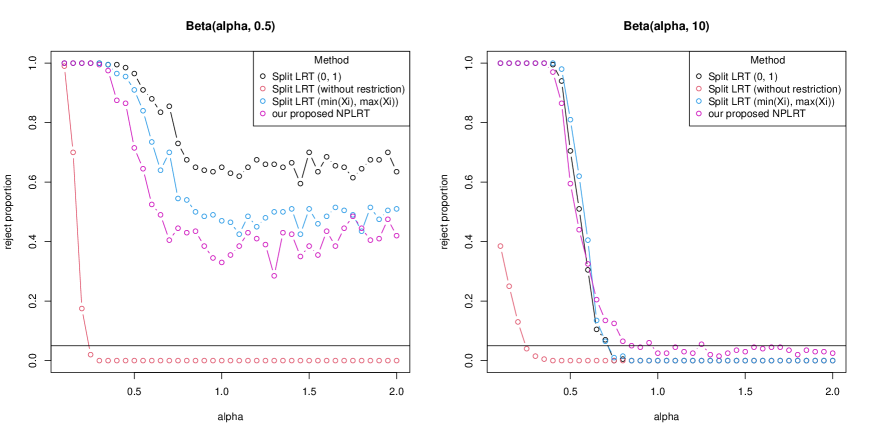
Figure 1: Comparison with the split LRT in [14]. The beta distribution with $\beta=0.5$ is not log-concave for any $\alpha$. The beta distribution with $\beta=10$ is log-concave only when $\alpha\geq 1$. The split LRT performs better when the true density is far from log-concave (see Figure 2). When the true density is closer to log-concave (see Figure 3), our proposed LRT has higher powers.

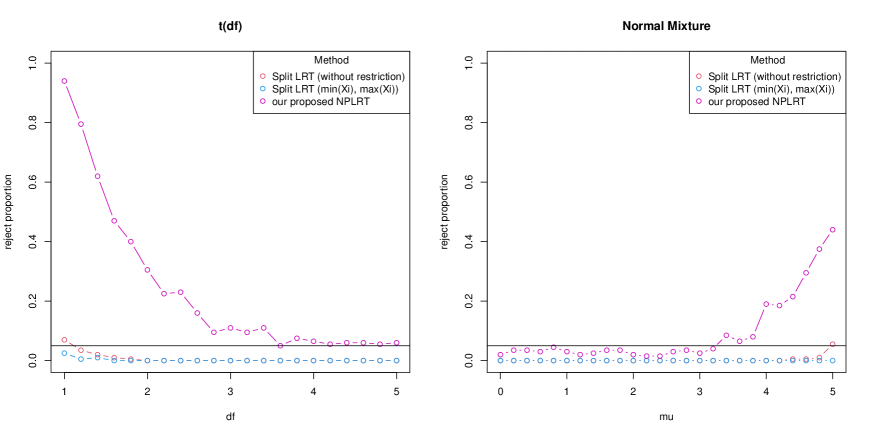
Figure 4: Comparison with the split LRT in [14]. The $t$-distribution with any degrees of freedom is not log-concave. The normal mixture $\frac{1}{2}\phi(x)+\frac{1}{2}\phi(x-\mu)$ is log-concave only when $\mu\leq 2$. Our proposed LRT has a higher power for all the $t$ distributions and normal mixtures when $\mu>2$.

We also compare our NPLRT with the fully nonparametric split LRT in [14]. The specification of the fully nonparametric split LRT requires an additional density estimator and we follow [14] to use a kernel density estimator (KDE). In particular, we follow [14] to use the kde1d function from the kde1d package in R, which allows user to restrict the support of the KDE. We compare the tests when the underlying random samples are from beta distributions, $t$-distributions and mixture of normal distributions. For the beta distributions, we consider three cases of support specification in kde1d: (i) $[0,1$], the true support; (ii) $[\min_{i}X_{i},\max_{i}X_{i}]$, an estimated support; and (iii) without any restriction. As in [14], we only compare the tests with $n=100$ and set the number of subsamples used in the split LRT to be $B=100$, and use $500$ independent replications to determine the rejection proportions. Figure 1 shows the results for the beta distributions. We see that the split LRT has a higher power when the true density is far from being log-concave but our NPLRT has a higher power when the true density is closer to, but not, being log-concave; see Figures 2 and 3 for the shapes of the corresponding log densities. Furthermore, the performance of the split LRT with KDE relies on a good specification of the support. When the support is not provided in kde1d, the powers drop significantly, possibly because of the well-known boundary issue of the KDE. For $t$-distributions and mixture of normals, our NPLRT outperforms the split LRT with KDE in all the scenarios; see Figure 4 for details.

		$n$	LRTA	LRTB	Trace	Split1	Split2	Split3
$H_{0}$	Exp(1)	100	0.05	0.06	0.19	0.00	0.00	0.00
		250	0.05	0.06	0.16	0.00	0.00	0.00
	N(0,1)	100	0.03	0.05	0.02	0.00	0.00	0.00
		250	0.04	0.05	0.01	0.00	0.00	0.00
	U(0,1)	100	0.03	0.05	0.08	0.00	0.00	0.00
		250	0.04	0.06	0.08	0.00	0.00	0.00
$H_{1}$	t(2)	100	0.28	0.28	0.88	0.00	0.00	0.00
		250	0.44	0.42	0.99	0.04	0.00	0.04
	Mix(5)	100	0.44	0.54	0.99	0.05	0.00	0.05
		250	0.82	0.87	1.00	0.99	0.36	0.99

Table 1: LRT_A and LRT_B refer to our LRT using the asymptotic null distribution and bootstrap procedure for finding the critical values, respectively. Trace refers to the test in [7]. Split1, Split2, and Split3 are the split LRT ([14]) by making use of the true support, $(\min_{i}X_{i},\max_{i}X_{i})$ as the support and without support restriction in the KDE. Mix(5) denotes the normal mixture with density $1/2\phi(x)+1/2\phi(x-5)$, where $\phi$ is the standard normal density.

6 Discussion

In this paper, we studied a nonparametric likelihood ratio test for univariate shape-constrained densities. The classes of $k$-monotonicity, complete monotonicity, and log-concavity were studied in detail. A universal asymptotic null distribution is derived and a bootstrap simulation procedure for finding the null distribution is shown to be valid. In the following, we discuss some additional remarks and possible extensions.

First, the NPLRT proposed in this article is not restricted to testing the classes of $k$-monotone, completely monotone, and log-concave densities. It is also valid for testing parametric classes of densities where we usually have $\frac{1}{n}\sum^{n}_{i=1}\log\frac{\hat{f}_{n}(X_{i})}{f_{0}(X_{i})}=O_{P}(n^{-1})$. It can also be applied to other nonparametric class of densities that may not be shape-constrained, for instance, the class of $\alpha$-Holder densities:

$$\mathcal{P}_{\alpha}:=\{f:[0,1]\rightarrow\mathbb{R},|f(x)-f(y)|\leq M|x-y|^{\alpha},x,y\in[0,1]\},$$

where $M>0$ and $\alpha>0$. If $f_{0}$ is bounded from below and $\alpha>1/2$, one can obtain the rate $h(\hat{f}_{n},f_{0})=O_{p}(n^{-\alpha/(2\alpha+1)})$ and $\frac{1}{n}\sum^{n}_{i=1}\log\frac{\hat{f}_{n}(X_{i})}{f_{0}(X_{i})}=O_{p}(n^{-2\alpha/(2\alpha+1)})$; see Example 7.4.6 in [42]. Thus, $S_{1n}=o_{p}(1)$ under the null, therefore the asymptotic null distribution would be valid. On the other hand, when $\alpha<1/2$, [5] showed that the rate of convergence of MLE in Hellinger distance is not better than $(n(\log n))^{-\alpha/2}$. In this case, Theorem 2.1 does not apply because $S_{1n}$ becomes the dominating term under $H_{0}$.

While the likelihood ratio test requires a modification because the MLE for the class of all densities do not exist, such a modification is unnecessary when a smaller class of alternatives is used in which the MLE exists. For instance, suppose we want to test the hypothesis that $H_{0}:f_{0}$ is $2$-monotone versus $H_{1}:f_{0}$ is $1$-monotone. Then, the log-likelihood ratio

$$\Lambda_{n1}:=-\frac{1}{n}\log\frac{\prod^{n}_{i=1}\hat{f}_{n,2}(X_{i})}{\prod^{n}_{i=1}\hat{f}_{n,1}(X_{i})}$$

is well-defined. We can expand $S_{1n}$ as

$$\Lambda_{n1}=\frac{1}{n}\sum^{n}_{i=1}\log\frac{\hat{f}_{n_{1}}(X_{i})}{f_{0}(X_{i})}-\frac{1}{n}\sum^{n}_{i=1}\log\frac{\hat{f}_{n,2}(X_{i})}{f_{0}(X_{i})}.$$

In Theorem 3.3, under some regularity conditions, we already know $\frac{1}{n}\sum^{n}_{i=1}\log\frac{\hat{f}_{n}(X_{i})}{f_{0}(X_{i})}=O_{p}(n^{-2/3})$ and $\frac{1}{n}\sum^{n}_{i=1}\log\frac{\hat{f}_{n,2}(X_{i})}{f_{0}(X_{i})}=O_{p}(n^{-4/5})$. Therefore, to determine the asymptotic distribution of $\Lambda_{n2}$, it suffices to study $\frac{1}{n}\sum^{n}_{i=1}\log\frac{\hat{f}_{n,1}(X_{i})}{f_{0}(X_{i})}$. In Theorem 4.1, we have shown that

$$\frac{1}{\sqrt{n}}\sum^{n}_{i=1}\log\frac{\hat{f}_{n,1}(X_{i})}{f_{0}(X_{i})}=(\mu^{2}_{2,f_{0}}+\kappa_{f_{0}})n^{-1/6}+O_{p}(n^{-1/3+\delta}).$$

A more detailed analysis is needed to establish its asymptotic distribution. However, the limiting distribution will depends on $f_{0}$ and a bootstrap procedure is in general needed to calibrate the test.

A multivariate extension of the current approach may proceed as follows. For simplicity, consider the bivariate case. Let $(X_{1},Y_{1}),\ldots,(X_{n},Y_{n})$ be a random sample from a bivaraite density $f_{0}$. In view of the expansion of $\Lambda_{n}$ in (3), we may generalize the definition for the bivariate case to

$$\Lambda_{n2}:=-\frac{1}{n}\sum^{n}_{i=1}\log\hat{f}_{n}(X_{i},Y_{i})-\frac{1}{n}\sum^{n}_{i=1}\log(X_{(i)}-X_{(i-1)})-\frac{1}{n}\sum^{n}_{i=1}\log(Y_{(i)}-Y_{(i-1)})-\log n^{2},$$

where $X_{(i)}$’s and $Y_{(i)}$’s are the order statistics of $X_{i}$’s and $Y_{i}$’s, respectively. We can then write $\Lambda_{n2}=K_{n2}+R_{n}$, where

$$K_{n2} := -\frac{1}{n}\sum^{n}_{i=1}\log\frac{\hat{f}_{n}(X_{i},Y_{i})}{f_{0}(X_{i},Y_{i})}$$

$$R_{n} := -\frac{1}{n}\sum^{n}_{i=1}\log\frac{f_{0}(X_{i},Y_{i})}{f^{X}_{0}(X_{i})f^{Y}_{0}(Y_{i})}-\frac{1}{n}\sum^{n}_{i=1}\log\frac{f^{X}_{0}(X_{i})(X_{(i)}-X_{(i-1)})}{1/n}$$

$$\quad-\frac{1}{n}\sum^{n}_{i=1}\log\frac{f^{Y}_{0}(Y_{i})(Y_{(i)}-Y_{(i-1)})}{1/n}.$$

Note that $\sqrt{n}(R_{n}-\mu_{0})$ should converge to some limit that depends on the true distribution, where $\mu_{0}$ depends on $f_{0}$. However, unless $X$ and $Y$ are independent, the distribution-freeness of the universal test will be lost. However, a bootstrap procedure is likely to remain valid. If $\sqrt{n}K_{n2}=o_{p}(1)$ as in [28] and [17], then the asymptotic distribution of $\Lambda_{n2}$ will be the same as that of $R_{n}$.

7 Appendix for Section 2

Proof of Equation (2).

First, it suffices to consider $f\in\mathcal{F}_{n}$ with $f(Z_{i})>0$ (otherwise $L_{n}(f)=0$). Let $a_{i}:=f(Z_{i})(Z_{i}-Z_{i-1})$ for $i=1,\ldots,n$. Then $\sum^{n}_{i=1}a_{i}=1$. Using the AM-GM inequality, we have

$$L_{n}(f)=\prod^{n}_{i=1}f(Z_{i})=\frac{\prod^{n}_{i=1}a_{i}}{\prod^{n}_{i=1}(Z_{i}-Z_{i-1})}\leq\frac{(\frac{1}{n}\sum^{n}_{i=1}a_{i})^{n}}{\prod^{n}_{i=1}(Z_{i}-Z_{i-1})}=\frac{1}{n^{n}\prod^{n}_{i=1}(Z_{i}-Z_{i-1})}.$$

Thus, the maximum value of $L_{n}$ is obtained when $a_{1}=\ldots=a_{n}=\frac{1}{n}$. ∎

7.1 Proof of Main Results

Proof of Theorem 2.1.

Because of the expansion in (3), $S_{1n}=o_{p}(1)$, and $S_{3n}=o_{p}(1)$, it remains to show that

$$\sqrt{n}\bigg{(}-\frac{1}{n}\sum^{n}_{i=1}\log\frac{F_{0}(Z_{i})-F_{0}(Z_{i-1})}{1/n}-\gamma\bigg{)}\stackrel{{\scriptstyle d}}{{\rightarrow}}N\bigg{(}0,\frac{\pi^{2}}{6}-1\bigg{)}.$$ (15)

The desired result then follows from Slutsky’s theorem. For (15), first note that

$$(F_{0}(Z_{1}),\ldots,F_{0}(Z_{n}))\stackrel{{\scriptstyle d}}{{=}}(U_{(1)},\ldots,U_{(n)}),$$

where $U_{(i)}$’s are the order statistics from a random sample from Uniform$(0,1)$ with sample size $n$. Then (15) follows from a result in [10] (p.249); see also [40] for more general results. ∎

For completeness, a proof of (15) is given below.

Proof of Equation (15).

Let

$$J_{n}:=-\frac{1}{n}\sum^{n}_{i=1}\log\frac{F_{0}(Z_{i})-F_{0}(Z_{i-1})}{1/n}.$$

Note that $(F_{0}(Z_{1}),\ldots,F_{0}(Z_{n}))$ and $(U_{(1)},\ldots,U_{(n)})$ have the same distribution, where $U_{(i)}$’s are the order statistics from a random sample from Uniform$(0,1)$ with the sample size $n$. Note that

$$(U_{(1)},U_{(2)}-U_{(1)},\ldots,U_{(n)}-U_{(n-1)})\stackrel{{\scriptstyle d}}{{=}}\bigg{(}\frac{E_{1}}{\sum^{n+1}_{h=1}E_{h}},\ldots,\frac{E_{n}}{\sum^{n+1}_{h=1}E_{h}}\bigg{)},$$

where $E_{h}$’s are independent random variables each of which is following the standard exponential distribution with the mean $=1$; see for example, Theorem 2.2 in [11]. Hence,

$$J_{n}\stackrel{{\scriptstyle d}}{{=}}-\frac{1}{n}\sum^{n}_{i=1}\log\bigg{\{}n\bigg{(}\frac{E_{i}}{\sum^{n+1}_{h=1}E_{h}}\bigg{)}\bigg{\}}=-\frac{1}{n}\sum^{n}_{i=1}\log E_{i}+\log\bigg{(}\frac{1}{n}\sum^{n+1}_{h=1}E_{h}\bigg{)}.$$

By the central limit theorem and Taylor’s theorem,

$$\log\bigg{(}\frac{1}{n}\sum^{n+1}_{h=1}E_{h}\bigg{)} = \log\bigg{[}1+\bigg{\{}\frac{1}{n}\sum^{n+1}_{h=1}(E_{h}-1)+\frac{1}{n}\bigg{\}}\bigg{]}=\frac{1}{n}\sum^{n+1}_{h=1}(E_{h}-1)+\frac{1}{n}+O_{p}\left(n^{-1}\right)$$

$$= \frac{1}{n}\sum^{n}_{h=1}(E_{h}-1)+O_{p}\left(n^{-1}\right).$$

Therefore, by the central limit theorem,

$$\sqrt{n}(J_{n}-\gamma)\stackrel{{\scriptstyle d}}{{=}}-\frac{\sqrt{n}}{n}\sum^{n}_{i=1}\bigg{(}(\log E_{i}-E_{i}+1)+\gamma\bigg{)}+O_{p}\left(n^{-1/2}\right)\stackrel{{\scriptstyle d}}{{\rightarrow}}N\bigg{(}0,\frac{\pi^{2}}{6}-1\bigg{)},$$

as each $\log E_{i}-E_{i}+1$ has mean $-\gamma$ and variance $\pi^{2}/6-1$, for $i=1,\ldots,n$. ∎

Proof of Theorem 2.2.

Fix $c\geq 0,\varepsilon>0$ and $\delta>0$. From the conditions that $\lim_{n\rightarrow\infty}\mathbb{P}(S_{1n}>L_{n})=1$ and $S_{3n}=o_{p}(1)$, for all sufficiently large $n$, we have

$$\mathbb{P}_{H_{1}}\bigg{(}\bigg{|}\frac{1}{\sqrt{n}}\sum^{n}_{i=1}\log\frac{f_{0}(Z_{i})(Z_{i}-Z_{i-1})}{F_{0}(Z_{i})-F_{0}(Z_{i-1})}\bigg{|}<\delta\bigg{)}>1-\frac{\varepsilon}{3}$$

and

$$\mathbb{P}_{H_{1}}\bigg{(}-\frac{1}{\sqrt{n}}\sum^{n}_{i=1}\log\frac{\hat{f}_{n}(X_{i})}{f_{0}(X_{i})}>L_{n}\bigg{)}>1-\frac{\varepsilon}{3}.$$

Furthermore, from the asymptotic normality in (15) (note that this holds regardless if $f_{0}\in\mathcal{F}$ or not), there exists $K>0$ such that for all sufficiently large $n$,

$$\mathbb{P}_{H_{1}}\bigg{(}\bigg{|}\sqrt{n}\bigg{(}-\frac{1}{n}\sum^{n}_{i=1}\log\frac{F_{0}(Z_{i})-F_{0}(Z_{i-1})}{1/n}-\gamma\bigg{)}\bigg{|}<K\bigg{)}>1-\frac{\varepsilon}{3}.$$

Hence, in view of (5) and the fact that $L_{n}\uparrow\infty$, for all sufficiently large $n$,

$$1-\varepsilon<\mathbb{P}_{H_{1}}(\sqrt{n}(\Lambda_{n}-\gamma)>-K-\delta+L_{n})\leq\mathbb{P}_{H_{1}}(\sqrt{n}(\Lambda_{n}-\gamma)>c),$$

and the claim follows as desired.

∎

7.2 Proof of Sufficient Conditions for Conditions B1 and B2

To prove Proposition 2.1, we first establish Lemmas 7.1 - 7.3.

Lemma 7.1.

Let $X_{1},\ldots,X_{n}$ be a random sample with the common density $f$ with $Z_{i}$’s being the corresponding order statistics with $Z_{0}:=\tau_{f}$. Suppose that one in list (b) of Proposition 2.1 holds. We have the following statements for some constant $C>0$ which is independent of $n$ but only depends on $f$:

1. Regardless of the value of $\tau_{f}$,

   $$\bigg{|}\sum^{n}_{i=2}\log\frac{f(Z_{i})(Z_{i}-Z_{i-1})}{F(Z_{i})-F(Z_{i-1})}\bigg{|}\leq C+2|\log f(Z_{1})|+2|\log f(Z_{n})|;$$ (16)

2. If $\tau_{f}$ is finite and known so that $f(\tau_{f}+)>0$, then

   $$\bigg{|}\sum^{n}_{i=1}\log\frac{f(Z_{i})(Z_{i}-Z_{i-1})}{F(Z_{i})-F(Z_{i-1})}\bigg{|}\leq C+2|\log f(Z_{n})|;$$ (17)

3. If $\tau_{f}$ is finite and known so that $f(\tau_{f}+)=0$, then

   $$\bigg{|}\sum^{n}_{i=1}\log\frac{f(Z_{i})(Z_{i}-Z_{i-1})}{F(Z_{i})-F(Z_{i-1})}\bigg{|} \leq C+3|\log f(Z_{1})|+2|\log f(Z_{n})|+|\log(Z_{1}-\tau_{f})|$$

   $$\quad+O_{p}(\log n).$$

Proof of Lemma 7.1.

1. 1. Consider the case that Condition (b)(I) in Proposition 2.1 holds. By the mean value theorem, for each $i$, there exists $\tilde{Z}_{i}\in(Z_{i-1},Z_{i})$ such that $F(Z_{i})-F(Z_{i-1})=f(\tilde{Z}_{i})(Z_{i}-Z_{i-1})$. Hence,

      $$\left|\sum^{n}_{i=2}\log\frac{f(Z_{i})(Z_{i}-Z_{i-1})}{F(Z_{i})-F(Z_{i-1})}\right| = \left|\sum^{n}_{i=2}\log\frac{f(Z_{i})}{f(\tilde{Z}_{i})}\right|\leq\left|\sum^{n}_{i=2}\log\frac{f(Z_{i})}{f(Z_{i-1})}\right|$$ (18)

      $$\leq |\log f(Z_{1})|+|\log f(Z_{n})|.$$

      Thus, (16) holds for any $C>0$.

   2. Consider the case that Condition (b)(II) in Proposition 2.1 holds. By the mean value theorem, for each $i$, there exists $\tilde{Z}_{i}\in(Z_{i-1},Z_{i})$ such that $F(Z_{i})-F(Z_{i-1})=f(\tilde{Z}_{i})(Z_{i}-Z_{i-1})$. Hence,

      $$\left|\sum^{n}_{i=2}\log\frac{f(Z_{i})(Z_{i}-Z_{i-1})}{F(Z_{i})-F(Z_{i-1})}\right|=\left|\sum^{n}_{i=2}\log\frac{f(Z_{i})}{f(\tilde{Z}_{i})}\right|$$ (19)

      $$= \Bigg{|}\sum_{i:Z_{i},\tilde{Z}_{i}\in[K_{1},K_{2}]}\log\frac{f(Z_{i})}{f(\tilde{Z}_{i})}+\sum_{i:Z_{i},\tilde{Z}_{i}<K_{1}}\log\frac{f(Z_{i})}{f(\tilde{Z}_{i})}+\sum_{i:Z_{i},\tilde{Z}_{i}>K_{2}}\log\frac{f(Z_{i})}{f(\tilde{Z}_{i})}$$

      $$\quad+\sum_{i:\tilde{Z}_{i}<K_{1}<Z_{i}}\log\frac{f(Z_{i})}{f(\tilde{Z}_{i})}+\sum_{i:\tilde{Z}_{i}<K_{2}<Z_{i}}\log\frac{f(Z_{i})}{f(\tilde{Z}_{i})}\Bigg{|}.$$

      For the first term on the RHS of (19),

      $$\Bigg{|}\sum_{i:Z_{i},\tilde{Z}_{i}\in[K_{1},K_{2}]}\log\frac{f(Z_{i})}{f(\tilde{Z}_{i})}\Bigg{|}\leq\sum_{i:Z_{i},\tilde{Z}_{i}\in[K_{1},K_{2}]}L(Z_{i}-\tilde{Z}_{i})\leq L(K_{2}-K_{1}).$$

      For the second term in the RHS of (19), if $f$ is increasing on $(-\tau_{f},K_{1}]$ , then

      $$0<\sum_{i:Z_{i},\tilde{Z}_{i}<K_{1}}\log\frac{f(Z_{i})}{f(\tilde{Z}_{i})}<\sum_{i:Z_{i},\tilde{Z}_{i}<K_{1}}\log\frac{f(Z_{i})}{f(Z_{i-1})}\leq\log f(K_{1})-\log f(Z_{1}).$$

      If $f$ is decreasing on $(-\tau_{f},K_{1}]$, then

      $$\log f(K_{1})-\log f(Z_{1})<\sum_{i:Z_{i},\tilde{Z}_{i}<K_{1}}\log\frac{f(Z_{i})}{f(Z_{i-1})}<\sum_{i:Z_{i},\tilde{Z}_{i}<K_{1}}\log\frac{f(Z_{i})}{f(\tilde{Z}_{i})}<0.$$

      Hence,

      $$\left|\sum_{i:Z_{i},\tilde{Z}_{i}<K_{1}}\log\frac{f(Z_{i})}{f(\tilde{Z}_{i})}\right|\leq|\log f(K_{1})|+|\log f(Z_{1})|.$$

      Similarly, for the third term in the RHS of (19),

      $$\left|\sum_{i:Z_{i},\tilde{Z}_{i}>K_{2}}\log\frac{f(Z_{i})}{f(\tilde{Z}_{i})}\right|\leq|\log f(K_{2})|+|\log f(Z_{n})|.$$

      Let $K^{*}_{1}$ be the index such that $\tilde{Z}_{K^{*}_{1}}<K_{1}<Z_{K^{*}_{1}}$. For the fourth term on the RHS of (19), we have

      $$\Bigg{|}\sum_{i:\tilde{Z}_{i}<K_{1}<Z_{i}}\log\frac{f(Z_{i})}{f(\tilde{Z}_{i})}\Bigg{|} = |\log f(Z_{K^{*}_{1}})-\log f(K_{1})+\log f(K_{1})-\log f(\tilde{Z}_{K^{*}_{1}})|$$

      $$\leq L(K_{2}-K_{1})+|\log f(K_{1})|+|\log f(Z_{1})|.$$

      Of course, when there is no such $i$ such that $\tilde{Z}_{i}<K_{1}<Z_{i}$, the above upper bound is still valid as the LHS is simply $0$. Similarly, for the fifth term in the RHS of (19), we have

      $$\bigg{|}\sum_{i:\tilde{Z}_{i}<K_{2}<Z_{i}}\log\frac{f(Z_{i})}{f(\tilde{Z}_{i})}\bigg{|}\leq L(K_{2}-K_{1})+|\log f(K_{2})|+|\log f(Z_{n})|.$$

      To conclude, (16) holds for any $C\geq 3L(K_{2}-K_{1})+2|\log f(K_{1})|+2|\log f(K_{2})|$.

2. 1. Consider the case that Condition (b)(I) in Proposition 2.1 holds. Similar to (i) (a), we now have

      $$\left|\sum^{n}_{i=1}\log\frac{f(Z_{i})(Z_{i}-Z_{i-1})}{F(Z_{i})-F(Z_{i-1})}\right| = \left|\sum^{n}_{i=1}\log\frac{f(Z_{i})}{f(\tilde{Z}_{i})}\right|\leq\left|\sum^{n}_{i=1}\log\frac{f(Z_{i})}{f(Z_{i-1})}\right|$$ (20)

      $$\leq |\log f(\tau_{f}+)|+|\log f(Z_{n})|.$$

      Thus, (17) holds for any $C\geq|\log f(\tau_{f}+)|$.

   2. Consider the case that Condition (b)(II) in Proposition 2.1 holds. The proof is similar to (i) (b) except that we now have

      $$\left|\sum_{i\geq 1:Z_{i},\tilde{Z}_{i}<K_{1}}\log\frac{f(Z_{i})}{f(\tilde{Z}_{i})}\right|\leq|\log f(K_{1})|+|\log f(\tau_{l}+)|.$$

      Hence, we can take $C\geq 3L(K_{2}-K_{1})+2|\log f(K_{1})|+2|\log f(K_{2})|+|\log f(\tau_{f}+)|$.

3. Since $f(\tau_{f}+)=0$, we cannot use the bound as in the proof of (ii). Instead, we write

   $$\sum^{n}_{i=1}\log\frac{f(Z_{i})(Z_{i}-Z_{i-1})}{F(Z_{i})-F(Z_{i-1})}=\sum^{n}_{i=2}\log\frac{f(Z_{i})(Z_{i}-Z_{i-1})}{F(Z_{i})-F(Z_{i-1})}+\log\frac{f(Z_{1})(Z_{1}-\tau_{f})}{F(Z_{1})}.$$

   Regardless of which Condition (b)(I)-(II) in Proposition 2.1 $f$ satisfies, using the result in (i), we have

   $$\bigg{|}\sum^{n}_{i=1}\log\frac{f(Z_{i})(Z_{i}-Z_{i-1})}{F(Z_{i})-F(Z_{i-1})}\bigg{|} \leq C+3|\log f(Z_{1})|+2|\log f(Z_{n})|+|\log(Z_{1}-\tau_{l})|$$

   $$\quad+|\log F(Z_{1})|.$$

   Note that $|\log F(Z_{1})|=O_{p}(\log n)$; indeed, we have

   $$\mathbb{P}(|\log F(Z_{1})|\leq x) = \mathbb{P}(\log U_{(1)}\geq-x)=\mathbb{P}(U_{(1)}\geq e^{-x})=\{\mathbb{P}(U_{1}\geq e^{-x})\}^{n}$$

   $$= (1-e^{-x})^{n},$$

   where $U_{1},\ldots,U_{n}$ are i.i.d. standard uniform random variables on $[0,1]$ with $U_{(1)}:=\min_{i=1,\ldots,n}U_{i}$. By taking $x=2\log n$, we have

   $$\lim_{n\rightarrow\infty}\mathbb{P}\bigg{(}|\log F(Z_{1})|\leq 2\log n\bigg{)}=1.$$

∎

The following lemma provides sufficient conditions for deriving the orders of

$$\frac{1}{n}\sum^{n}_{i=1}\log f(X_{i}),\log f(Z_{1})\text{ and }\log f(Z_{n}).$$

Lemma 7.2.

Let $X_{1},X_{2},\ldots$ be a sequence of random variables that are identically distributed with a common density $f$ but not necessarily independent of each other.

1. Suppose that $\int_{\mathbb{R}}f(x)^{1-\alpha}dx<\infty$ for some $\alpha>0$. Then

   $$\mathbb{P}\bigg{(}\limsup_{n\rightarrow\infty}\max_{i=1,\ldots,n}[-\{\log f(X_{i})\}(\log n)^{-1}]\leq\frac{2}{\alpha}\bigg{)}=1.$$ (21)

2. Suppose that $\int_{\mathbb{R}}f(x)^{1+\alpha}dx<\infty$ for some $\alpha>0$. Then

   $$\mathbb{P}\bigg{(}\limsup_{n\rightarrow\infty}\max_{i=1,\ldots,n}[\{\log f(X_{i})\}(\log n)^{-1}]\leq\frac{2}{\alpha}\bigg{)}=1.$$ (22)

Proof of Lemma 7.2.

We only prove (21) while (22) could be proven similarly and we omit it. First, observe that

$$\mathbb{E}[f(X_{1})^{-\alpha}]=\int_{\mathbb{R}}f(x)^{1-\alpha}dx<\infty.$$

By Markov’s inequality, for any $m>1$,

$$\mathbb{P}(f(X_{n})^{-\alpha}>n^{m})\leq\frac{\mathbb{E}(f(X_{n})^{-\alpha})}{n^{m}}=\frac{\mathbb{E}(f(X_{1})^{-\alpha})}{n^{m}}.$$

Hence,

$$\sum^{\infty}_{n=1}\mathbb{P}(f(X_{n})^{-\alpha}>n^{m})\leq\mathbb{E}(f(X_{1})^{-\alpha})\sum^{\infty}_{n=1}\frac{1}{n^{m}}<\infty.$$

By the first Borel-Cantelli lemma, with the probability one, there exists an integer $N_{1}$ such that for all $n\geq N_{1}$,

$$f(X_{n})^{-\alpha}\leq n^{m}.$$

There also exists another integer $N_{2}\geq N_{1}$ such that for all $i=1,\ldots,N_{2}$, $f(X_{i})^{-\alpha}\leq N^{m}_{2}$. In other words, for all $n\geq N_{2}$ and $i\leq n$, $f(X_{i})^{-\alpha}\leq n^{m}$. Hence, with probability one,

$$\limsup_{n\rightarrow\infty}\max_{i=1,\ldots,n}[-\{\log f(X_{i})\}(\log n)^{-1}]\leq\frac{m}{\alpha}$$

and (21) follows by taking $m=2$.

∎

Lemma 7.3.

Let $X_{1},X_{2},\ldots$ be a sequence of random variables that are identically distributed with a common density $f$ but not necessarily independent of each other. Suppose that $\tau_{f}$ is finite. If $\int^{\infty}_{\tau_{f}}(x-\tau_{f})^{-\beta}f(x)dx<\infty$ for some $\beta>0$, then $\log(Z_{1}-\tau_{f})=O_{p}(\log n)$.

Proof of Lemma 7.3.

By Markov’s inequality,

$$\mathbb{P}((X_{n}-\tau_{f})^{-\beta}>n^{2})\leq\frac{\mathbb{E}((X_{n}-\tau_{f})^{-\beta})}{n^{2}}.$$

Hence,

$$\sum^{\infty}_{n=1}\mathbb{P}((X_{n}-\tau_{f})^{-\beta}>n^{2})\leq\mathbb{E}((X_{1}-\tau_{f})^{-\beta})\sum^{\infty}_{n=1}\frac{1}{n^{2}}<\infty.$$

By the first Borel-Cantelli lemma, with probability one, there exists $N_{1}$ such that for all $n\geq N_{1}$,

$$(X_{n}-\tau_{f})^{-\beta}\leq n^{2}.$$

There also exists another integer $N_{2}\geq N_{1}$ such that for all $i=1,\ldots,N_{2}$, $(X_{i}-\tau_{f})^{-\beta}\leq N^{2}_{2}$. In other words, for all $n\geq N_{2}$, and $i\leq n$, $(X_{i}-\tau_{f})^{-\beta}\leq n^{2}$. Thus, with the probability one,

$$\limsup_{n\rightarrow\infty}\{-\log(Z_{1}-\tau_{f})(\log n)^{-1}\}\leq 2/\beta.$$

This implies that $\log(Z_{1}-\tau_{f})=O_{p}(\log n)$. ∎

Proof of Proposition 2.1.

First, when (a) holds, regardless of the value of $\tau_{f}$, we have

$$\frac{1}{n}\sum^{n}_{i=1}\log f(X_{i})\leq\max_{i=1,\ldots,n}\log f(X_{i})\text{ and }-\frac{1}{n}\sum^{n}_{i=1}\log f(X_{i})\leq\max_{i=1,\ldots,n}\{-\log f(X_{i})\}.$$

Therefore, by Lemma 7.2, we have with the probability one,

$$\limsup_{n\rightarrow\infty}\bigg{|}\frac{1}{n}\sum^{n}_{i=1}\log f(X_{i})\bigg{|}(\log n)^{-1}\leq\frac{2}{\alpha}.$$

This implies that $\frac{1}{n}\sum^{n}_{i=1}\log f(X_{i})=O_{p}(\log n)$. Similarly, note that

$$\log f(Z_{1})\leq\max_{i=1,\ldots,n}f(X_{i})\text{ and }-\log f(Z_{1})\leq\max_{i=1,\ldots,n}\{-\log f(X_{i})\}.$$

By Lemma 7.2 again, we have $\log f(Z_{1})=O_{p}(\log n)$. The same argument also lead to $\log f(Z_{n})=O_{p}(\log n)$.

1. From the above results, the first two terms in $S^{\prime}_{3n}$ are $O_{p}((\log n)/\sqrt{n})$. As one in list (b) holds, by Lemma 7.1 (i) together with $\log f(Z_{1})=O_{p}(\log n)$ and $\log f(Z_{n})=O_{p}(\log n)$, the last term in $S^{\prime}_{3n}$ is also $O_{p}((\log n)/\sqrt{n})$.

2. When one in list (b) and (c)(I) hold, $S_{3n}=O_{p}((\log n)/\sqrt{n})$ in view of Lemma 7.1 (ii) together with $\log f(Z_{n})=O_{p}(\log n)$. When one in list (b) and (c)(II) hold, $S_{3n}=O_{p}((\log n)/\sqrt{n})$ in view of Lemma 7.1 (iii), Lemma 7.3 together with $\log f(Z_{1})=O_{p}(\log n)$ and $\log f(Z_{n})=O_{p}(\log n)$.

∎

Proof of Corollary 2.1.

We shall show that the conditions in Proposition 2.1 are satisfied so that the result follows. First, a log-concave density must be unimodal. It is either monotone over the support, or there exists $K_{1}>\tau_{f}$ and $K_{2}<\sigma_{f}$ such that $f_{0}$ is monotone on $(\tau_{f},K_{1}]$ and $[K_{2},\sigma_{f})$. Furthermore, because $\log f_{0}$ is concave, $\log f_{0}$ is Lipschitz continuous on $[K_{1},K_{2}]$. To show $\int_{\mathbb{R}}f_{0}(x)^{1\pm\alpha}dx<\infty$ for some $\alpha>0$, simply note that log-concave density has an exponential tail (see Lemma 1 in [8]), that is, there exist $a>0$ and $b\in\mathbb{R}$ such that $f_{0}(x)\leq e^{-a|x|+b}$ for all $x$. Finally, if $f_{0}(\tau_{f}+)=0$, then for some $\delta>0$, $\int^{\infty}_{\tau_{f}}(x-\tau_{f})^{-\beta}f_{0}(x)\leq\int^{\tau_{f}+\delta}_{\tau_{f}}(x-\tau_{f})^{-\beta}e^{b}dx+\int^{\infty}_{\tau_{f}+\delta}(x-\tau_{f})^{-\beta}e^{-a|x|+b}dx<\infty$, for any reasonably small $\beta(<1)$. ∎

8 Appendix for Section 3

8.1 $k$-monotone Densities

To prove Lemmas 3.1 and 3.2, we first recall that the MLE $\hat{f}_{n,k}$ is of the form

$$\hat{f}_{n,k}(x)=\sum^{m}_{j=1}\hat{w}_{j}\frac{k(\hat{a}_{j}-x)^{k-1}_{+}}{\hat{a}^{k}_{j}},$$ (23)

where $m\in\mathbb{Z}^{+}$, and $\{\hat{w}_{1},\ldots,\hat{w}_{m}\}$ and $\{\hat{a}_{1},\ldots,\hat{a}_{m}\}$ are respectively the family of weights and support points of the maximizing mixing distribution corresponding to $\hat{f}_{n,k}$, and $a_{+}$ denotes $\max(a,0)$ for any $a\in\mathbb{R}$; see Lemma 2 in [3]. Without loss of generality, we can assume that $\hat{a}_{1}\leq\ldots\leq\hat{a}_{m}$. The likelihood function at $\hat{f}_{n,k}$ is

$$L_{n}(\hat{f}_{n,k})=\prod^{n}_{i=1}\bigg{\{}\sum^{m}_{j=1}\hat{w}_{j}\frac{k(\hat{a}_{j}-X_{i})^{k-1}_{+}}{\hat{a}^{k}_{j}}\bigg{\}}.$$

Proof of Lemma 3.1.

We first show that $\hat{f}_{n,k}(0+)=O_{p}(1)$ if $f_{0}$ is bounded from above. Proposition 6 in [18] shows that when $f_{0}\in\mathcal{F}_{k}^{B}([0,A])$, we have $\hat{f}_{n,k}(0+)=O_{p}(1)$. A closer inspection on their proof reveals that the main step is to make use of the characterization of the MLE, which does not rely on the boundedness of the support of $f_{0}$. Hence, the same proof remains valid in this case.

Now, we shall show that, in general, $\hat{f}_{n,k}(0+)\leq kZ^{-1}_{1}$. For $k=1$, $\hat{f}_{n,1}(0)Z_{1}=\int^{Z_{1}}_{0}\hat{f}_{n,k}(x)dx\leq\int^{\infty}_{0}\hat{f}_{n}(x)dx=1$. Therefore, $\hat{f}_{n}(0)\leq Z^{-1}_{1}$. For $k\geq 2$, we make use of the form in (23) and claim that $\hat{a}_{1}>Z_{1}$. To see that, fix the values of $\hat{a}_{2},\ldots,\hat{a}_{m}$ and $\hat{w}_{1},\ldots,\hat{w}_{m}$, if $\hat{a}_{1}\leq Z_{1}$, then $(\hat{a}_{1}-X_{i})^{k-1}_{+}=0$ for all $i$ while if $\hat{a}_{1}>Z_{1}$, $(\hat{a}-X_{i})_{+}^{k-1}>0$ for some $i$. Hence, the maximum value of $L_{n}$ must be obtained when $\hat{a}_{1}>Z_{1}$. Finally, from the proof of Proposition 6 in [18], we have

$$\hat{f}_{n,k}(0)\leq\frac{k\mathbb{F}_{n}(\hat{a}_{1})}{\hat{a}_{1}}\leq\frac{k}{Z_{1}}.$$

∎

Proof of Lemma 3.2.

For $k=1$, it is well-known that $\sigma_{\hat{f}_{n,1}}=Z_{n}$. In the rest of this proof, we assume that $k\geq 2$. In view of (23), $\hat{a}_{m}=\sigma_{\hat{f}_{n,k}}$. For fixed $\hat{a}_{1},\ldots,\hat{a}_{m-1}$ and $\hat{w}_{1},\ldots,\hat{w}_{m}$, we investigate how the change of $\hat{a}_{m}$ affects the value of the likelihood. By the definition of the MLE, we know that $\hat{a}_{m}>Z_{n}$ since $k\geq 2$ (see also Remark 2 in [3]). Therefore, for each $i$, we shall consider the term

$$\hat{w}_{m}\frac{k(\hat{a}_{m}-X_{i})^{k-1}_{+}}{\hat{a}^{k}_{m}}.$$ (24)

Consider the function $g_{i}(y)=\frac{(y-X_{i})^{k-1}}{y^{k}}$ for $y>X_{i}$. Then,

$$g^{\prime}_{i}(y)=\frac{(y-X_{i})^{k-2}}{y^{k+1}}(kX_{i}-y)\text{ for }y>X_{i},$$

with which we can see that $g_{i}$ increases and then decreases in $y$, and attains its maximum at $kX_{i}$. Therefore, if $\hat{a}_{m}>kZ_{n}$, the term in (24) becomes smaller for all $i=1,\ldots,n$ if $\hat{a}_{m}$ is set at a larger value. This shows that the optimality can be ensured only if $\hat{a}_{m}\leq kZ_{n}$. ∎

Proof of Theorem 3.3.

We shall only prove (i). The other cases can be proven similarly. Fix $k\in\mathbb{N}$. For simplicity, we write $\hat{f}_{n}$ instead of $\hat{f}_{n,k}$. From the proof of Lemma 4.1 and Lemma 4.2 in [42], we have

$$0 \leq -\frac{1}{4}K_{n,k}\leq\frac{1}{2}\int\log\frac{\hat{f}_{n}+f_{0}}{2f_{0}}d(\mathbb{F}_{n}-F_{0})-h^{2}\left(\frac{\hat{f}_{n}+f_{0}}{2},f_{0}\right)$$

$$\leq \frac{1}{2}\int\log\frac{\hat{f}_{n}+f_{0}}{2f_{0}}d(\mathbb{F}_{n}-F_{0})-\frac{1}{16}h^{2}\left(\hat{f}_{n},f_{0}\right).$$

Let $m_{f}(t):=\log\frac{f(t)+f_{0}(t)}{2}$. Fix $M>0$. Let $\delta_{n}:=n^{-\frac{k}{2k+1}}|\log(a_{n}b_{n})|^{\frac{1}{2(2k+1)}}$. Then, we have

$$\mathbb{P}\left(-\frac{\sqrt{n}}{2}K_{n,k}\geq\sqrt{n}2^{2M}\delta^{2}_{n}\right)$$

$$\leq \mathbb{P}\left(\mathbb{G}_{n}(m_{\hat{f}_{n}})-\frac{\sqrt{n}}{8}h^{2}(\hat{f}_{n},f_{0})\geq\sqrt{n}2^{2M}\delta^{2}_{n},kZ^{-1}_{1}\leq a_{n},kZ_{n}\leq b_{n}\right)$$

$$\quad+\mathbb{P}(kZ^{-1}_{1}>a_{n})+\mathbb{P}(kZ_{n}>b_{n}),$$

where the last two terms in the last display go to $0$ as $n$ goes to infinity by assumptions on $a_{n}$ and $b_{n}$. Using the peeling device, we obtain

$$A_{n} := \mathbb{P}\left(\mathbb{G}_{n}(m_{\hat{f}_{n}})-\frac{\sqrt{n}}{8}h^{2}(\hat{f}_{n},f_{0})\geq\sqrt{n}2^{2M}\delta^{2}_{n},kZ^{-1}_{1}\leq a_{n},kZ_{n}\leq b_{n}\right)$$

$$\leq \sum^{S_{n}}_{s=0}\mathbb{P}\left(\sup_{f\in\mathcal{F}^{a_{n}}_{k}([0,b_{n}]):2^{M+s}\delta_{n}\leq h(f,f_{0})<2^{M+s+1}\delta_{n}}\left(\mathbb{G}_{n}(m_{f})-\frac{\sqrt{n}}{8}h^{2}(f,f_{0})\right)\geq\sqrt{n}2^{2M}\delta^{2}_{n}\right)$$

$$\quad+\mathbb{P}\left(\sup_{f\in\mathcal{F}^{a_{n}}_{k}([0,b_{n}]):h(f,f_{0})<2^{M}\delta_{n}}\left(\mathbb{G}_{n}(m_{f})-\frac{\sqrt{n}}{8}h^{2}(f,f_{0})\right)\geq\sqrt{n}2^{2M}\delta^{2}_{n}\right)$$

$$\leq \sum^{S_{n}}_{s=0}\mathbb{P}\left(\sup_{f\in\mathcal{F}^{a_{n}}_{k}([0,b_{n}]):2^{M+s}\delta_{n}\leq h(f,f_{0})<2^{M+s+1}\delta_{n}}\mathbb{G}_{n}(m_{f})\geq\sqrt{n}2^{2M}(2^{2s}+1)\delta^{2}_{n}\right)$$

$$\quad+\mathbb{P}\left(\sup_{f\in\mathcal{F}^{a_{n}}_{k}([0,b_{n}]):h(f,f_{0})<2^{M}\delta_{n}}\mathbb{G}_{n}(m_{f})\geq\sqrt{n}2^{2M}\delta^{2}_{n}\right)$$

$$\leq \sum^{S_{n}}_{s=0}\mathbb{P}\left(\sup_{f\in\mathcal{F}^{a_{n}}_{k}([0,b_{n}]):h(f,f_{0})<2^{M+s+1}\delta_{n}}\mathbb{G}_{n}(m_{f})\geq\sqrt{n}2^{2M}2^{2s}\delta^{2}_{n}\right)$$

$$\quad+\mathbb{P}\left(\sup_{f\in\mathcal{F}^{a_{n}}_{k}([0,b_{n}]):h(f,f_{0})<2^{M}\delta_{n}}\mathbb{G}_{n}(m_{f})\geq\sqrt{n}2^{2M}\delta^{2}_{n}\right)$$

where $S_{n}:=\min\{s:2^{M+s+1}\delta_{n}\geq 1\}$. Define

$$\mathcal{M}_{n,\delta}:=\left\{m_{f}:f\in\mathcal{F}^{a_{n}}_{k}([0,b_{n}]),h(f,f_{0})<\delta\right\}.$$

By Markov’s inequality,

$$A_{n} \leq \sum^{S_{n}}_{s=0}\frac{\mathbb{E}||\mathbb{G}_{n}||_{\mathcal{M}_{n,2^{M+s+1}\delta_{n}}}}{\sqrt{n}2^{2M}2^{2s}\delta^{2}_{n}}+\frac{\mathbb{E}||\mathbb{G}_{n}||_{\mathcal{M}_{n,2^{M}\delta_{n}}}}{\sqrt{n}2^{2M}\delta^{2}_{n}},$$

where $\mathbb{E}||\mathbb{G}_{n}||_{\mathcal{M}_{n,\delta}}:=\sup_{f\in\mathcal{M}_{n,\delta}}\mathbb{E}|\mathbb{G}_{n}(f)|$. By Theorem 3.4.4 in [43],

$$\mathbb{E}||\mathbb{G}_{n}||_{\mathcal{M}_{n,\delta}}\lesssim\tilde{J}_{[\cdot]}(\delta,\mathcal{F}^{a_{n}}_{k}([0,b_{n}]),h)\left(1+\frac{\tilde{J}_{[\cdot]}(\delta,\mathcal{F}^{a_{n}}_{k}([0,b_{n}]),h)}{\delta^{2}\sqrt{n}}\right).$$

From (7), we have

$$\log N_{[\cdot]}(\delta,\mathcal{F}^{a_{n}}_{k}([0,b_{n}]),h)\leq C_{k}|\log(a_{n}b_{n})|^{\frac{1}{2k}}\delta^{-\frac{1}{k}}.$$

A direct calculation gives

$$\tilde{J}_{[\cdot]}\left(\delta,\mathcal{F}_{k}^{a_{n}}([0,b_{n}]),h\right)\lesssim C_{k}^{1/2}|\log(a_{n}b_{n})|^{\frac{1}{4k}}\frac{\delta^{1-\frac{1}{2k}}}{1-\frac{1}{2k}}\lesssim|\log(a_{n}b_{n})|^{\frac{1}{4k}}\delta^{1-\frac{1}{2k}}$$ (25)

for all large enough $n$ as $C_{k}$ only depends on $k$. Define

$$\xi_{n}(\delta):=|\log(a_{n}b_{n})|^{\frac{1}{4k}}\delta^{1-\frac{1}{2k}}\left(1+\frac{|\log(a_{n}b_{n})|^{\frac{1}{4k}}\delta^{1-\frac{1}{2k}}}{\delta^{2}\sqrt{n}}\right).$$

Note that $\xi_{n}(\delta)/\delta$ is decreasing in $\delta$ for any fixed $n$. Thus, for any $j>0$,

$$\frac{\xi_{n}(2^{j}\delta_{n})}{\delta^{2}_{n}}\leq\frac{2^{j}\xi_{n}(\delta_{n})}{\delta^{2}_{n}}=2^{j+1}\sqrt{n}.$$

Hence,

$$A_{n} \lesssim \sum^{S_{n}}_{s=0}\frac{\xi_{n}(2^{M+s+1}\delta_{n})}{\sqrt{n}2^{2M}2^{2s}\delta^{2}_{n}}+\frac{\xi_{n}(2^{M}\delta_{n})}{\sqrt{n}2^{2M}\delta^{2}_{n}}\leq\sum^{\infty}_{s=0}\frac{2^{M+s+2}\sqrt{n}}{\sqrt{n}2^{2M}2^{2s}}+\frac{2^{M+1}\sqrt{n}}{\sqrt{n}2^{2M}}=\frac{10}{2^{M}},$$

which goes to $0$ as $M$ goes to $\infty$. ∎

Proof of Corollary 3.1.

We shall apply Theorem 2.1 by verifying $S_{1n}=o_{p}(1)$ and $S_{3n}=o_{p}(1)$ (when $\tau_{f}$ is known) or $S^{\prime}_{3n}=o_{p}(1)$ (when $\tau_{f}$ is unknown). First, as $a_{n}b_{n}=o\left(\exp\left(n^{\frac{2k-1}{2}}\right)\right)$, $S_{1n}=o_{p}(1)$ as a result of Theorem 3.3. As $\int^{\infty}_{0}f_{0}(x)^{1\pm\alpha}dx<\infty$ for some $\alpha>0$ and $f_{0}$ is decreasing, $S_{3n}=o_{p}(1)$ also holds by Proposition 2.1 (ii), and therefore

$$\sqrt{n}(\Lambda_{n}-\gamma)\stackrel{{\scriptstyle d}}{{\rightarrow}}N(0,\pi^{2}/6-1),\quad\text{as }n\rightarrow\infty,$$

by Theorem 2.1. Similarly, by Proposition 2.1 (i), $S^{\prime}_{3n}=o_{p}(1)$ also holds and therefore

$$\sqrt{n}(\Lambda^{\prime}_{n}-\gamma)\stackrel{{\scriptstyle d}}{{\rightarrow}}N(0,\pi^{2}/6-1),\quad\text{as }n\rightarrow\infty,$$

as in Theorem 2.1; see also the remark following Theorem 2.2. ∎

Proof of Theorem 3.4.

Let $\varepsilon:=\inf_{f\in\mathcal{F}_{k}}h(f,f_{0})>0$. Also let $c_{j}$, $j=1,\ldots,4$, be the positive constants in Theorem 1 in [46]. First, note that

$$\mathbb{P}\bigg{(}\prod^{n}_{i=1}\frac{\hat{f}_{n,k}(X_{i})}{f_{0}(X_{i})}\geq e^{-c_{1}n\varepsilon^{2}}\bigg{)}$$

$$\leq \mathbb{P}\bigg{(}\prod^{n}_{i=1}\frac{\hat{f}_{n,k}(X_{i})}{f_{0}(X_{i})}\geq e^{-c_{1}n\varepsilon^{2}},\hat{f}_{n,k}\in\mathcal{F}^{a_{n}}_{k}[0,b_{n}]\bigg{)}+\mathbb{P}(\hat{f}_{n,k}\notin\mathcal{F}^{a_{n}}_{k}[0,b_{n}])$$

$$\leq \mathbb{P}\bigg{(}\sup_{f\in\mathcal{F}^{a_{n}}_{k}[0,b_{n}]}\prod^{n}_{i=1}\frac{f(X_{i})}{f_{0}(X_{i})}\geq e^{-c_{1}n\varepsilon^{2}}\bigg{)}+\mathbb{P}(\hat{f}_{n,k}\notin\mathcal{F}^{a_{n}}_{k}[0,b_{n}]).$$

To verify (3.1) in [46], we have, using Theorem 3 in [18],

$$\int^{\sqrt{2}\varepsilon}_{\frac{\varepsilon^{2}}{2^{8}}}\sqrt{\log N_{[\cdot]}\bigg{(}\frac{u}{c_{3}},\mathcal{F}^{a_{n}}_{k}([0,b_{n}]),h\bigg{)}}du \leq \int^{\sqrt{2}\varepsilon}_{0}C^{\frac{1}{2}}_{k}|\log(a_{n}b_{n})|^{\frac{1}{4k}}\bigg{(}\frac{u}{c_{3}}\bigg{)}^{-\frac{1}{2k}}du$$

$$\leq C^{\frac{1}{2}}_{k}c_{3}^{\frac{1}{2k}}2^{\frac{1}{2}-\frac{1}{4k}}\varepsilon^{1-\frac{1}{2k}}|\log(a_{n}b_{n})|^{\frac{1}{4k}}.$$

As $a_{n}b_{n}=o(\exp(n^{2k}))$, the right hand side of the last inequality is smaller than $c_{4}n^{1/2}\varepsilon^{2}$ for all large enough $n$. Therefore, by Theorem 1 in [46], for all large enough $n$,

$$\mathbb{P}\bigg{(}\sup_{f\in\mathcal{F}^{a_{n}}_{k}[0,b_{n}]}\prod^{n}_{i=1}\frac{f(X_{i})}{f_{0}(X_{i})}\geq e^{-c_{1}n\varepsilon^{2}}\bigg{)}\leq 4\exp(-c_{2}n\varepsilon^{2}).$$

Hence,

$$\limsup_{n\rightarrow\infty}\mathbb{P}\bigg{(}\prod^{n}_{i=1}\frac{\hat{f}_{n,k}(X_{i})}{f_{0}(X_{i})}\geq e^{-c_{1}n\varepsilon^{2}}\bigg{)} \leq \limsup_{n\rightarrow\infty}4\exp(-c_{2}n\varepsilon^{2})+\limsup_{n\rightarrow\infty}\mathbb{P}(\hat{f}_{n,k}\notin\mathcal{F}^{a_{n}}_{k}([0,b_{n}]))$$

$$= \limsup_{n\rightarrow\infty}\mathbb{P}(\hat{f}_{n,k}\notin\mathcal{F}^{a_{n}}_{k}([0,b_{n}]))=0,$$

as $\hat{f}_{n,k}\in\mathcal{F}^{a_{n}}_{k}([0,b_{n}])$ with a probability going to $1$. Finally, this implies that

$$\lim_{n\rightarrow\infty}\mathbb{P}\bigg{(}\frac{1}{n}\sum^{n}_{i=1}\log\frac{f_{0}(X_{i})}{\hat{f}_{n,k}(X_{i})}>c_{1}\varepsilon^{2}\bigg{)}=\lim_{n\rightarrow\infty}\mathbb{P}\bigg{(}\prod^{n}_{i=1}\frac{\hat{f}_{n,k}(X_{i})}{f_{0}(X_{i})}<e^{-c_{1}n\varepsilon^{2}}\bigg{)}=1.$$

∎

Proof of Corollary 3.2.

First, by Theorem 3.4, there exists $L_{n}\uparrow\infty$ such that $\lim_{n\rightarrow\infty}\mathbb{P}(S_{1n}>L_{n})=1$.

1. By Proposition 2.1 (ii), $S_{3n}=o_{p}(1)$. Therefore, by Theorem 2.2, the NPLRT using $\Lambda_{n}$ is consistent.

2. By Proposition 2.1 (i), $S_{3n}^{\prime}=o_{p}(1)$. Therefore, the NPLRT using $\Lambda_{n}^{\prime}$ is consistent as in (i); see also the remark following Theorem 2.2.

∎

8.2 Completely Monotone Densities

Proof of Lemma 3.5.

For simplicity, we write $\hat{f}_{n}$ instead of $\hat{f}_{n,\infty}$. First, from [27], we know that the MLE is of the form

$$\hat{f}_{n}(t)=\sum^{r_{n}}_{i=1}\hat{\lambda}_{i}\hat{p}_{i}e^{-\hat{\lambda}_{i}t},$$

for some $r_{n}\leq n$, $\sum^{r_{n}}_{i=1}\hat{p}_{i}=1$ and $\hat{\lambda}_{i}\in[Z_{n}^{-1},Z_{1}^{-1}]$ for each $i=1,\ldots,r_{n}$. Without loss of generality, we simply assume that $\hat{\lambda}_{1}\leq\ldots\leq\hat{\lambda}_{r_{n}}$. We shall first obtain an upper bound of $\hat{f}_{n}$ for a large $t$. Note that

$$\hat{f}_{n}(t)\leq\sum^{r_{n}}_{i=1}\hat{p}_{i}\max_{j=1,\ldots,r_{n}}\hat{\lambda}_{j}e^{-\hat{\lambda}_{j}t}=\max_{j=1,\ldots,r_{n}}\hat{\lambda}_{j}e^{-\hat{\lambda}_{j}t},$$

as $\sum^{r_{n}}_{i=1}\hat{p}_{i}=1$. For any fixed $t$, the function $\lambda\mapsto\lambda e^{-\lambda t}$ is unimodal and achieves maximum when $\lambda=1/t$. Thus, if $t>Z_{n}$ so that $1/t<1/Z_{n}\leq\hat{\lambda}_{1}$, we have

$$\hat{f}_{n}(t)\leq\hat{\lambda}_{1}e^{-\hat{\lambda}_{1}t}\leq\frac{1}{Z_{n}}e^{-\frac{t}{Z_{n}}}.$$

Since $f_{0}$ has an unbounded support, $Z_{n}\stackrel{{\scriptstyle a.s.}}{{\rightarrow}}\infty$. Thus, with a probability approaching to $1$, we have $c_{2n}\geq Z^{1+\beta}_{n}>Z_{n}$ and for all $t>c_{2n}$,

$$\hat{f}_{n}(t)\leq\frac{1}{Z_{n}}e^{-\frac{t}{Z_{n}}}\leq\frac{1}{t^{2}}\quad\text{ as }n\rightarrow\infty.$$ (26)

We shall also obtain a rough upper bound for $\hat{f}_{n}(0)$. Observe that

$$\hat{f}_{n}(0)=\sum^{r_{n}}_{i=1}\hat{\lambda}_{i}\hat{p}_{i}\leq\sum^{r_{n}}_{i=1}\hat{p}_{i}\max_{j=1,\ldots,r_{n}}\hat{\lambda}_{j}\leq\max_{j=1,\ldots,r_{n}}\hat{\lambda}_{j}\leq Z^{-1}_{1}.$$

To obtain a rate of convergence of $\hat{f}_{n}$, we shall find an upper bound for the bracketing entropy of a class of functions where the MLE will be in with a probability approaching to $1$. To this end, write

$$\hat{f}_{n}(t)=\hat{f}_{n}(t)I(t\leq c_{2n})+\hat{f}_{n}(t)I(t>c_{2n}).$$

Define

$$\tilde{\mathcal{F}}_{n}:=\tilde{\mathcal{F}}^{c_{1n}}_{1}([0,c_{2n}])+\mathcal{G}_{n},$$

where

$$\tilde{\mathcal{F}}^{c_{1n}}_{1}([0,c_{2n}]):=\left\{f:[0,c_{2n}]\rightarrow\mathbb{R}^{+}:\text{$f$ is decreasing},\int^{c_{2n}}_{0}f(x)dx\leq 1,f(0)\leq c_{1n}\right\}.$$

and

$$\mathcal{G}_{n}:=\left\{f:(c_{2n},\infty)\rightarrow[0,1]:\text{$f$ is decreasing, }f(t)\leq 1/t^{2}\right\}.$$

Because of (10), $\lim_{n\rightarrow\infty}\mathbb{P}(\hat{f}_{n}(t)I(t\leq c_{2n})\in\tilde{\mathcal{F}}^{c_{1n}}_{1}([0,c_{2n}])=1$. In view of (26), we have $\lim_{n\rightarrow\infty}\mathbb{P}(\hat{f}_{n}(t)I(t>c_{2n})\in\mathcal{G}_{n})=1$. Therefore,

$$\lim_{n\rightarrow\infty}\mathbb{P}(\hat{f}_{n}\in\tilde{\mathcal{F}}_{n})=1.$$ (27)

We shall now show that $\tilde{\mathcal{F}}_{n}$ has a finite bracketing entropy with respect to Hellinger distance. First, from the proof of Theorem 3 in [18], we know the result of that theorem is also valid for $\tilde{\mathcal{F}}^{c_{1n}}_{1}([0,c_{2n}])$, where for any function $f$ in this class such that $\int^{c_{2n}}_{0}f(x)dx\leq 1$ rather than just $\int^{c_{2n}}_{0}f(x)dx=1$. Thus,

$$\log N_{[\cdot]}(\varepsilon,\tilde{\mathcal{F}}^{c_{1n}}_{1}([0,c_{2n}]),h)\leq C|\log(c_{1n}c_{2n})|^{1/2}\varepsilon^{-1},$$ (28)

where $C$ is a universal constant. Then, note that if $f\in\mathcal{G}_{n}$, then $f^{1/2}\in\mathcal{G}^{1/2}_{n}$, where

$$\mathcal{G}^{1/2}_{n}:=\left\{f:(c_{2n},\infty)\rightarrow[0,1]:\text{$f$ is decreasing, }f(t)\leq 1/t\right\}.$$

As $\int^{\infty}_{c_{2n}}1/x^{2(1-\gamma)}dx<\infty$ for some $\gamma\in(0,1)$, we can apply the idea of Lemma 7.10 in [42] to obtain that

$$\log N_{[\cdot]}(\varepsilon,\mathcal{G}^{1/2}_{n},||\cdot||_{2})\leq A\varepsilon^{-1},$$ (29)

where $A$ is a universal constant and $||\cdot||_{2}$ is the $L^{2}$-norm with respect to the Lebesgue measure on $[0,\infty)$. Now, simply note that

$$\log N_{[\cdot]}(\varepsilon,\mathcal{G}^{1/2}_{n},||\cdot||_{2})=\log N_{[\cdot]}(\varepsilon,\mathcal{G}_{n},h).$$ (30)

Combining (28) to (30), we obtain that

$$\log N_{[\cdot]}(\varepsilon,\tilde{\mathcal{F}}_{n},h)\leq\{C|\log(c_{1n}c_{2n})|^{1/2}+A\}\varepsilon^{-1}\lesssim|\log(c_{1n}c_{2n})|^{1/2}\varepsilon^{-1},$$ (31)

for all large $n$. With (27) and (31), we can obtain (12) as in the proof of Theorem 3.3 and we omit the details. ∎

The proof of Corollary 3.3 is similar to that of Corollary 3.1 for $k$-monotone densities and is therefore omitted. The proofs of Theorem 3.6 and Corollary 3.4 are similar to those of Theorem 3.4 and Corollary 3.2 for $k$-monotone densities and are therefore omitted.

8.3 Log-concave Densities

Proof of Theorem 3.7.

The proof is similar to the one in Theorem 3.4, where we apply the large deviation inequality in Theorem 1 in [46]. To this end, it suffices to verify (3.1) in [46] and our claim then follows as a result. Without loss of generality, assume that the interval $[-1,1]$ is strictly contained in the support of $f_{0}$. Because $\int_{\mathbb{R}}|x|f_{0}(x)dx<\infty$, by Lemma 3 in [9], $\hat{f}_{n,lc}\in\mathcal{F}^{M}_{lc}$ for some $M>0$ with a probability approaching to $1$ as $n\rightarrow\infty$. By Theorem 3.1 in [12], $\log N_{[\cdot]}(u/c_{3},\mathcal{F}^{M}_{lc},h)\precsim u^{-1/2}$. Hence,

$$\int^{\sqrt{2}\varepsilon}_{\frac{\varepsilon^{2}}{2^{8}}}\sqrt{\log N_{[\cdot]}\bigg{(}\frac{u}{c_{3}},\mathcal{F}^{M}_{lc},h\bigg{)}}du\precsim\int^{\sqrt{2}{\varepsilon}}_{0}u^{-1/4}du\precsim\varepsilon^{3/4}.$$

Thus, the right hand side of the last inequality is smaller than $c_{4}n^{1/2}\varepsilon^{2}$ for all large enough $n$, and so (3.1) in [46] is satisfied. ∎

Proof of Corollary 3.6.

First, by Theorem 3.7, there exists $L_{n}\uparrow\infty$ such that $\lim_{n\rightarrow\infty}\mathbb{P}(S_{1n}>L_{n})=1$.

1. By Proposition 2.1 (ii), $S_{3n}=o_{p}(1)$. Therefore, by Theorem 2.2, the NPLRT using $\Lambda_{n}$ is consistent.

2. By Proposition 2.1 (i), $S_{3n}^{\prime}=o_{p}(1)$. Therefore, the NPLRT using $\Lambda_{n}^{\prime}$ is consistent as in (i); see also the remark following Theorem 2.2.

∎

9 Appendix for Section 4

9.1 Proof of Theorem 4.1

For the sake of simplicity, we write $\hat{f}_{n}$ for $\hat{f}_{n,1}$ in this section. Recall that $\hat{\mathbb{F}}_{n}$ denotes the least concave majorant of the empirical distribution function $\mathbb{F}_{n}$. To prove Theorem 4.1, we write

$$\frac{1}{\sqrt{n}}\sum^{n}_{i=1}\log\frac{\hat{f}_{n}(X_{i})}{f_{0}(X_{i})} = \sqrt{n}\int_{0}^{1}\log\frac{\hat{f}_{n}(t)}{f_{0}(t)}\,d\hat{\mathbb{F}}_{n}(t)+\sqrt{n}\int_{0}^{1}\log\frac{\hat{f}_{n}(t)}{f_{0}(t)}\,d\{\mathbb{F}_{n}(t)-\hat{\mathbb{F}}_{n}(t)\}$$

$$=: A_{n}+B_{n}.$$

Here, $A_{n}$ can be viewed as the Kullback–Leibler divergence of $f_{0}$ from $\hat{f}_{n}$ and so $A_{n}$ is nonnegative by a simple application of Jensen’s inequality. The following Lemma 9.1 will demonstrate that $A_{n}$ is asymptotically equivalent to a weighted $L_{2}$-error between $\hat{f}_{n}$ and $f_{0}$, which is asymptotic normally distributed by a generalization of Theorem 1.1 in [30]; see Lemma 9.1. Lemma 9.2 will show that $B_{n}$ is also nonnegative and asymptotically equivalent to a weighted $L_{1}$-norm between $\hat{\mathbb{F}}_{n}$ and $\mathbb{F}_{n}$, which is also asymptotic normally distributed by Theorem 2.1 in [31].

Lemma 9.1.

Under the conditions in Theorem 4.1, we have

$$\sqrt{n}\int_{0}^{1}\log\frac{\hat{f}_{n}(t)}{f_{0}(t)}\,d\hat{\mathbb{F}}_{n}(t)=\sqrt{n}\int_{0}^{1}\frac{|\hat{f}_{n}(t)-f_{0}(t)|^{2}}{2f_{0}(t)}\,dt+O_{p}(n^{-1/3+\delta}),$$

for any $\delta>0$.

Lemma 9.2.

Under the conditions in Theorem 4.1, we have

$$\sqrt{n}\int_{0}^{1}\log\frac{\hat{f}_{n}(t)}{f_{0}(t)}\,d\{\mathbb{F}_{n}(t)-\hat{\mathbb{F}}_{n}(t)\}=\sqrt{n}\int_{0}^{1}\{\hat{\mathbb{F}}_{n}(t)-\mathbb{F}_{n}(t)\}\frac{|f_{0}^{\prime}(t)|}{f_{0}(t)}\,dt.$$

In addition,

$$\sqrt{n}\int_{0}^{1}\{\hat{\mathbb{F}}_{n}(t)-\mathbb{F}_{n}(t)\}\frac{|f_{0}^{\prime}(t)|}{f_{0}(t)}\,dt=\kappa_{f_{0}}n^{-1/6}+O_{p}(n^{-1/3}).$$

Remark.

Since $\hat{\mathbb{F}}_{n}$ is the least concave majorant of $\mathbb{F}_{n}$, $\hat{\mathbb{F}}_{n}\geq\mathbb{F}_{n}$. Thus, $\hat{\mathbb{F}}_{n}(t)-\mathbb{F}_{n}(t)=|\hat{\mathbb{F}}_{n}(t)-\mathbb{F}_{n}(t)|$ and so the term $\int^{1}_{0}\{\hat{\mathbb{F}}_{n}(t)-\mathbb{F}_{n}(t)\}|f^{\prime}_{0}(t)|/f_{0}(t)dt$ is a weighted $L_{1}$-norm of the difference between $\hat{\mathbb{F}}_{n}$ and $\mathbb{F}_{n}$.

We first provide Lemmas 9.3 - 9.5 that are used in the proof of Lemma 9.1.

Lemma 9.3.

Suppose that $f_{0}$ is a decreasing density with support on $[0,1]$ and $0<f_{0}(1)\leq f_{0}(0)<\infty$. Then, $1/\hat{f}_{n}(\hat{Z}_{n})=O_{p}(1)$. In other words, for any $\epsilon>0$, there exists $\delta>0$ such that for all sufficiently large $n$,

$$\mathbb{P}(\hat{f}_{n}(Z_{n})>\delta)>1-\epsilon.$$

Proof of Lemma 9.3.

From page 326-328 of [36], we know that

$$\hat{f}_{n}(Z_{n})=\min_{0\leq i\leq n-1}\frac{n-i}{n(Z_{n}-Z_{i})}.$$

Then

$$1/\hat{f}_{n}(Z_{n})=\max_{0\leq i\leq n-1}\frac{n(Z_{n}-Z_{i})}{n-i}=\max_{h=1,\ldots,n}\frac{n(Z_{n}-Z_{n-h})}{h}=O_{p}(1),$$

by Corollary 5.2 (i) in [6]. ∎

Lemma 9.4.

Under the conditions in Theorem 4.1, we have

$$~{}\sqrt{n}\int_{0}^{1}|\hat{f}_{n}(t)-f_{0}(t)|^{3}\,dt=O_{p}(n^{-1/3+\delta})$$

for any $\delta>0$.

Proof of Lemma 9.4.

For any $0<\delta^{\prime}<2.5$, we can bound this third-degree moment term by

$$~{}\int_{0}^{1}|\hat{f}_{n}(t)-f_{0}(t)|^{3}\,dt= ~{}\int_{0}^{1}\left|\hat{f}_{n}(t)-f_{0}(t)\right|^{2.5-\delta^{\prime}}\left|\hat{f}_{n}(t)-f_{0}(t)\right|^{0.5+\delta^{\prime}}\,dt$$

$$\leq ~{}[2\max\{f_{0}(0),\hat{f}_{n}(0+)\}]^{0.5+\delta^{\prime}}\int_{0}^{1}\left|\hat{f}_{n}(t)-f_{0}(t)\right|^{2.5-\delta^{\prime}}\,dt,$$

where $[2\max\{f_{0}(0),\hat{f}_{n}(0+)\}]^{0.5+\delta^{\prime}}=O_{p}(1)$. Theorem 1.1 in [30] with $k=2.5-\delta^{\prime}$ implies that

$$n^{1/6}\left[n^{1/3}\left\{\int_{0}^{1}\left|\hat{f}_{n}(t)-f_{0}(t)\right|^{2.5-\delta^{\prime}}\,dt\right\}^{1/(2.5-\delta^{\prime})}-\mu_{2.5-\delta^{\prime}}\right]=O_{p}(1),$$

for some finite constant $\mu_{2.5-\delta^{\prime}}$. By straightforward algebra, we have

$$\left\{\int_{0}^{1}\left|\hat{f}_{n}(t)-f_{0}(t)\right|^{2.5-\delta^{\prime}}\,dt\right\}^{1/(2.5-\delta^{\prime})}=O_{p}(n^{-1/2})+\mu_{2.5-\delta^{\prime}}n^{-1/3}=O_{p}(n^{-1/3})$$

and so

$$\int_{0}^{1}\left|\hat{f}_{n}(t)-f_{0}(t)\right|^{2.5-\delta^{\prime}}=O_{p}(n^{-5/6+\delta}),$$

where $\delta=\delta^{\prime}/3$ and the result in the lemma follows.

∎

It is indicated in Remark 1.1 in [30] that one may obtain the asymptotic normality of the following weighted version of the $L_{k}$-error of $\hat{f}_{n}$:

$$n^{1/6}\left\{n^{k/3}\int_{0}^{1}\frac{|\hat{f}_{n}(t)-f_{0}(t)|^{k}}{2f_{0}(t)}\,dt-\mu_{k,f_{0}}^{k}\right\},$$

for some $\mu_{k,f_{0}}>0$. We state such claim formally in Lemma 9.5 and omit the proof.

Lemma 9.5 (Modified version of Theorem 1.1 in [30]).

Under the conditions in Theorem 4.1, we have, for $1\leq k<2.5$,

$$n^{1/6}\left\{n^{k/3}\int_{0}^{1}\frac{|\hat{f}_{n}(t)-f_{0}(t)|^{k}}{2f_{0}(t)}\,dt-\mu_{k,f_{0}}^{k}\right\}$$

converges in distribution to a zero-mean normal random variable with a finite variance as $n\to\infty$, where

$$\mu_{k,f_{0}}:=\bigg{\{}\mathbb{E}|V(0)|^{k}\int^{1}_{0}2^{\frac{2k}{3}-1}f_{0}(t)^{\frac{k}{3}-1}|f^{\prime}_{0}(t)|^{\frac{k}{3}}dt\bigg{\}}^{\frac{1}{k}},$$

with $V(\cdot)$ defined in Theorem 4.1.

Proof of Lemma 9.1.

Using Taylor’s expansion, for some $f_{n}^{*}(t)$ lying between $f_{0}(t)$ and $\hat{f}_{n}(t)$, we have

$$\sqrt{n}\int_{0}^{1}\log\frac{\hat{f}_{n}(t)}{f_{0}(t)}\hat{f}_{n}(t)\,dt = \sqrt{n}\int_{0}^{1}\frac{\hat{f}_{n}(t)-f_{0}(t)}{f_{0}(t)}\hat{f}_{n}(t)\,dt-\sqrt{n}\int_{0}^{1}\frac{\{\hat{f}_{n}(t)-f_{0}(t)\}^{2}}{2f_{0}^{2}(t)}\hat{f}_{n}(t)\,dt$$

$$+\sqrt{n}\int_{0}^{1}\frac{\{\hat{f}_{n}(t)-f_{0}(t)\}^{3}}{3\{f_{n}^{*}(t)\}^{3}}\hat{f}_{n}(t)\,dt,$$

$$=: A_{n1}+A_{n2}+A_{n3}.$$

Interestingly, at the first glance, $A_{n1}$ and $A_{n2}$ do not share the same rate of convergence. However, they are equally important for the Kullback–Leibler divergence from $\hat{f}_{n}$ to $f_{0}$. In the following, we shall show that both $A_{n1}$ and $A_{n2}$ are related to a weighted $L_{2}$-error between $\hat{f}_{n}$ and $f_{0}$ asymptotically. For $A_{n3}$, it is relatively small and comparatively negligible.

1. For $A_{n1}$, because $\hat{f}_{n}$ and $f_{0}$ are both densities, we have $\int_{0}^{1}\{\hat{f}_{n}(t)-f_{0}(t)\}\,dt=0$. Thus,

   $$A_{n1}= ~{}\sqrt{n}\int_{0}^{1}\frac{\hat{f}_{n}(t)-f_{0}(t)}{f_{0}(t)}\hat{f}_{n}(t)\,dt-\sqrt{n}\int_{0}^{1}\{\hat{f}_{n}(t)-f_{0}(t)\}\frac{f_{0}(t)}{f_{0}(t)}\,dt$$

   $$= ~{}\sqrt{n}\int_{0}^{1}\frac{\{\hat{f}_{n}(t)-f_{0}(t)\}^{2}}{f_{0}(t)}\,dt.$$

2. For $A_{n2}$, we have

   $$A_{n2}= ~{}-\sqrt{n}\int_{0}^{1}\frac{\{\hat{f}_{n}(t)-f_{0}(t)\}^{2}}{2f_{0}(t)}\frac{\hat{f}_{n}(t)}{f_{0}(t)}\,dt$$

   $$= ~{}-\sqrt{n}\int_{0}^{1}\frac{\{\hat{f}_{n}(t)-f_{0}(t)\}^{2}}{2f_{0}(t)}\left\{\frac{f_{0}(t)}{f_{0}(t)}+\frac{\hat{f}_{n}(t)-f_{0}(t)}{f_{0}(t)}\right\}\,dt$$

   $$= ~{}-\sqrt{n}\int_{0}^{1}\frac{\{\hat{f}_{n}(t)-f_{0}(t)\}^{2}}{2f_{0}(t)}\,dt-\sqrt{n}\int_{0}^{1}\frac{\{\hat{f}_{n}(t)-f_{0}(t)\}^{3}}{2\{f_{0}(t)\}^{2}}\,dt.$$

   Under the conditions in Theorem 4.1, we can apply Lemma 9.4 to obtain that the second term in the last displayed equation is of the order $O_{p}(n^{-1/3+\delta})$ because $f_{0}(1)>0$.

3. We aim to show that $A_{n3}=O_{p}(n^{-1/3+\delta})$. Because $\hat{f}_{n}(t)=0$ when $t>Z_{n}$ and, for all $t$, $\hat{f}_{n}(t)\leq\hat{f}_{n}(0+)=O_{p}(1)$, the absolute value of $A_{n3}$ is bounded above by

   $$\sqrt{n}\int_{0}^{Z_{n}}\frac{|\hat{f}_{n}(t)-f_{0}(t)|^{3}}{3\{f_{n}^{*}(t)\}^{3}}\hat{f}_{n}(t)\,dt\leq O_{p}(1)\sqrt{n}\int_{0}^{Z_{n}}\frac{|\hat{f}_{n}(t)-f_{0}(t)|^{3}}{3\{f_{n}^{*}(t)\}^{3}}\,dt.$$

   Although $f_{n}^{*}(t)$ is lying between and $\hat{f}_{n}$ and $f_{0}$, where for all $t,f_{0}(t)\geq f_{0}(1)>0$, it is not guaranteed that $\hat{f}_{n}$ is bounded away from zero as well. By Lemma 9.3, we show that $1/\hat{f}_{n}(1)=O_{p}(1)$. As a result, we have

   $$\sqrt{n}\int_{0}^{Z_{n}}\frac{|\hat{f}_{n}(t)-f_{0}(t)|^{3}}{3\{f_{n}^{*}(t)\}^{3}}\,dt \leq \sqrt{n}\int^{Z_{n}}_{0}\frac{|\hat{f}_{n}(t)-f_{0}(t)|^{3}}{3\min\{\hat{f}_{n}(Z_{n})^{3},f_{0}(1)^{3}\}}dt$$

   $$\leq O_{p}(1)\sqrt{n}\int^{1}_{0}|\hat{f}_{n}(t)-f_{0}(t)|^{3}dt=O_{p}(n^{-1/3+\delta}),$$

   by Lemma 9.4.

Combining (i)-(iii), the claim in the lemma follows. ∎

Proof of Lemma 9.2.

First, from the proof of Lemma 4.2 in [26], we know

$$\int_{0}^{1}\log\hat{f}_{n}(t)\,d\mathbb{F}_{n}(t)=\int_{0}^{1}\log\hat{f}_{n}(t)\,\hat{\mathbb{F}}_{n}(t).$$

Therefore,

$$\int_{0}^{1}\log\frac{\hat{f}_{n}(t)}{f_{0}(t)}\,d\{\mathbb{F}_{n}(t)-\hat{\mathbb{F}}_{n}(t)\}=-\int_{0}^{1}\log f_{0}(t)\,d\{\mathbb{F}_{n}(t)-\hat{\mathbb{F}}_{n}(t)\}.$$ (32)

Also, because $\mathbb{F}_{n}$ and $\hat{\mathbb{F}}_{n}$ are both distribution functions over $[0,1]$, we have

$$\sqrt{n}\int_{0}^{1}\log f_{0}(0)\,d\{\mathbb{F}_{n}(t)-\hat{\mathbb{F}}_{n}(t)\}=0.$$

Thus,

$$-\int_{0}^{1}\log f_{0}(t)\,d\{\mathbb{F}_{n}(t)-\hat{\mathbb{F}}_{n}(t)\} = -\int_{0}^{1}\{\log f_{0}(t)-\log f_{0}(0)\}\,d\{\mathbb{F}_{n}(t)-\hat{\mathbb{F}}_{n}(t)\}$$ (33)

$$= \int_{0}^{1}\int_{0}^{t}\frac{|f_{0}^{\prime}(w)|}{f_{0}(w)}\,dw\,d\{\mathbb{F}_{n}(t)-\hat{\mathbb{F}}_{n}(t)\}$$

$$= \int_{0}^{1}\left[\int_{w}^{1}\,d\{\mathbb{F}_{n}(t)-\hat{\mathbb{F}}_{n}(t)\}\right]\frac{|f_{0}^{\prime}(w)|}{f_{0}(w)}\,dw$$

$$= \int_{0}^{1}\{\hat{\mathbb{F}}_{n}(w)-\mathbb{F}_{n}(w)\}\frac{|f_{0}^{\prime}(w)|}{f_{0}(w)}dw,$$

where the third equality holds by Fubini’s theorem. Under the conditions in Theorem 4.1, we can apply Theorem 2.1 in [31] to obtain that

$$n^{1/6}\left[n^{2/3}\int_{0}^{1}\{\hat{\mathbb{F}}_{n}(w)-\mathbb{F}_{n}(w)\}\frac{|f_{0}^{\prime}(w)|}{f_{0}(w)}dw-\kappa_{f_{0}}\right]$$

converges to a normal distribution with zero mean and a finite variance. The above convergence implies that

$$\int_{0}^{1}\{\hat{\mathbb{F}}_{n}(w)-\mathbb{F}_{n}(w)\}\frac{|f_{0}^{\prime}(w)|}{f_{0}(w)}dw=\kappa_{f_{0}}n^{-1/6}+O_{p}(n^{-1/3}),$$ (34)

where $\kappa_{f_{0}}$ is defined in Theorem 4.1. The claim in the lemma follows in view of (32), (33) and (34). ∎

Proof of Theorem 4.1.

By Lemmas 9.1 and 9.2,

$$\frac{1}{\sqrt{n}}\sum^{n}_{i=1}\log\frac{\hat{f}_{n}(X_{i})}{f_{0}(X_{i})}=-\sqrt{n}\int_{0}^{1}\frac{|\hat{f}_{n}(t)-f_{0}(t)|^{2}}{2f_{0}(t)}\,dt-\kappa_{f_{0}}n^{-1/6}+O_{p}(n^{-1/3+\delta}).$$

It remains to show that

$$\sqrt{n}\int_{0}^{1}\frac{|\hat{f}_{n}(t)-f_{0}(t)|^{2}}{2f_{0}(t)}\,dt=n^{-1/6}\mu_{2,f_{0}}^{2}+O_{p}(n^{-1/3+\delta}),$$

which is implied by Lemma 9.5.

∎

9.2 Convergence under a sequence of underlying distributions

To establish bootstrap consistency in Section 4, we have to consider the MLE under the setting that the samples are generated from a sequence of underlying distributions defined on a probability space $(\Omega,\mathcal{G},\mathbb{P})$. To this end, let $X_{n1},\ldots,X_{nn}$ be a random sample from $f_{n}$, a deterministic sequence of densities. Let $F_{n}$ be the distribution functions of $f_{n}$ and $\mathbb{F}_{nn}$ the empirical distribution from $X_{ni}$’s. Denote the corresponding order statistics of $X_{ni}$’s by $Z_{n1}\leq\ldots\leq Z_{nn}$. The $k$-monotone MLE, completely monotone MLE and log-concave MLE for $f_{n}$ from the sample $X_{ni}$’s are denoted by $\hat{f}_{nn,k}$, $\hat{f}_{nn,\infty}$ and $\hat{f}_{nn,lc}$, respectively. To prepare for the proofs of the bootstrap consistency in Theorems 9.10 - 9.12, we first provide upper bounds for $-\log f_{n}(Z_{n1})$ and $-\log f_{n}(Z_{nn})$ in the following Lemma 9.6, and establish the rates of convergence to $0$ of the respective $\hat{f}_{nn,k}$, $\hat{f}_{nn,\infty}$ and $\hat{f}_{nn,lc}$ in terms of the log-likelihood ratio to $f_{n}$ in Lemmas 9.7 to 9.9 when $f_{n}$ is $k$-monotone, completely monotone and log-concave, respectively. To indicate the dependence of a sample point $\omega$ in the sample space $\Omega$ in different functions, notations such as $Z_{nn}(\omega)$ and $\hat{f}_{nn,k}(\cdot;\omega)$ will also be used.

Lemma 9.6.

Let $f_{n}$ be a sequence of densities with $\tau_{f_{n}}>-\infty$.

1. If $f_{n}$ is unimodal and $\int^{\infty}_{-\infty}f^{1-\alpha}_{n}(x)dx\leq n^{m_{0}}$ for some $\alpha,m_{0}>0$ for all large $n$, then for some constant $C>0$,

   $$\mathbb{P}\left(\limsup_{n\rightarrow\infty}\frac{-\log\min\{f_{n}(Z_{n1}),f_{n}(Z_{nn})\}}{\log n}\leq C\right)=1.$$

2. If $\mathbb{E}((X_{n1}-\tau_{f_{n}})^{-\alpha})\leq n^{m_{0}}$ for some $\alpha,m_{0}>0$ for all large $n$, then for some constant $C>0$,

   $$\mathbb{P}\bigg{(}\limsup_{n\rightarrow\infty}\frac{-\log(Z_{n1}-\tau_{f_{n}})}{\log n}\leq C\bigg{)}=1.$$

Proof of Lemma 9.6.

1. Fix $m>m_{0}+1$. Then

   $$\mathbb{P}(\min\{f_{n}(Z_{n1}),f_{n}(Z_{nn})\}^{-\alpha}>n^{m}) = 1-\mathbb{P}(\min\{f_{n}(Z_{n1}),f_{n}(Z_{nn})\}^{-\alpha}\leq n^{m})$$

   $$= 1-\{\mathbb{P}(f^{-\alpha}_{n}(X_{n1})\leq n^{m})\}^{n}$$

   $$= 1-\{1-\mathbb{P}(f^{-\alpha}_{n}(X_{n1})>n^{m}))\}^{n}$$

   $$\leq 1-\left(1-\frac{\mathbb{E}(f^{-\alpha}_{n}(X_{n1}))}{n^{m}}\right)^{n}$$

   $$\leq 1-\left(1-\frac{n^{m_{0}}}{n^{m}}\right)^{n}$$

   $$\leq \frac{1}{n^{2}},$$

   where the second equality follows as $f_{n}$ is unimodal and the first inequality follows from Markov’s inequality. Hence, $\sum^{\infty}_{n=1}\mathbb{P}(\min\{f_{n}(Z_{n1}),f_{n}(Z_{nn})\}>n^{m})<\infty$. By the first Borel-Cantelli Lemma, with a probability one, for all large enough $n$, $\min\{f_{n}(Z_{n1}),f_{n}(Z_{nn})\}^{-\alpha}\leq n^{m}$ and the claim in the lemma follows with $C=m/\alpha>0$.

2. Fix $m>m_{0}+1$, by Markov’s inequality, we have for all large enough $n$,

   $$\mathbb{P}((Z_{n1}-\tau_{f_{n}})^{-\alpha}>n^{m}) = 1-\{1-\mathbb{P}((X_{n1}-\tau_{f_{n}})^{-\alpha}>n^{m})\}^{n}$$

   $$\leq 1-\bigg{\{}1-\frac{\mathbb{E}((X_{n1}-\tau_{f_{n}})^{-\alpha})}{n^{m}}\bigg{\}}^{n}$$

   $$\leq 1-\bigg{(}1-\frac{n^{m_{0}}}{n^{m}}\bigg{)}^{n}\leq\frac{1}{n^{2}}.$$

   Hence, $\sum^{\infty}_{n=1}\mathbb{P}((Z_{n1}-\tau_{f_{n}})^{-\alpha}>n^{m})<\infty$. By the first Borel-Cantelli Lemma, with the probability one, for all large enough $n$, $(Z_{n1}-\tau_{f_{n}})^{-\alpha}\leq n^{m}$ and the claim in the lemma follows with $C=m/\alpha>0$.

∎

Lemma 9.7 (for $k$-monotone densities).

Let $\{M_{n}\}$ and $\{\tilde{b}_{n}\}$ be sequences that can possibly go to $\infty$. Suppose that $f_{n}\in\mathcal{F}_{k}^{M_{n}}([0,\tilde{b}_{n}])$ for all large enough $n$. Then,

$$\frac{1}{\sqrt{n}}\sum^{n}_{i=1}\log\frac{\hat{f}_{nn,k}(X_{ni})}{f_{n}(X_{ni})}=O_{p}\left(n^{-\frac{2k-1}{2(2k+1)}}|\log(\widetilde{M}_{n}\tilde{b}_{n})|^{\frac{1}{2k+1}}\right),$$

where $\widetilde{M}_{n}$ satisfies $\widetilde{M}_{n}/M_{n}\rightarrow\infty$.

Proof of Theorem 9.7.

First, note that if $f_{n}\in\mathcal{F}_{k}^{M_{n}}([0,\tilde{b}_{n}])$, then $\hat{f}_{nn,k}(0+)=O_{p}(M_{n})$. To see that, following the proof of Proposition 6 in [18], we know that

$$\hat{f}_{nn,k}(0+)\leq k\sup_{t>0}\frac{\mathbb{F}_{nn}(t)}{F_{n}(t)}f_{n}(0+)=O_{p}(M_{n}),$$

since

$$\sup_{t>0}\frac{\mathbb{F}_{nn}(t)}{F_{n}(t)}=\sup_{0<t\leq 1}\frac{\mathbb{G}_{nn}(t)}{t}=O_{p}(1)$$

by Daniels’ theorem (see Theorem 2 on p. 345 in [41]), where

$$\mathbb{G}_{nn}(t):=\frac{1}{n}\sum^{n}_{i=1}I(F_{n}(X_{ni})\leq t).$$

Since $f_{n}\in\mathcal{F}_{k}^{M_{n}}([0,\tilde{b}_{n}])$, $Z_{nn}\leq\tilde{b}_{n}$. By Lemma 3.2, we also know $\sigma_{\hat{f}_{nn}}\leq kZ_{nn}$. Hence, $\sigma_{\hat{f}_{nn}}\leq k\tilde{b}_{n}$. Since $\widetilde{M}_{n}/M_{n}\rightarrow\infty$ by assumption, we then have

$$\lim_{n\rightarrow\infty}\mathbb{P}(\hat{f}_{nn,k}\notin\mathcal{F}^{\widetilde{M}_{n}}_{k}([0,k\tilde{b}_{n}]))=\lim_{n\rightarrow\infty}\mathbb{P}(\hat{f}_{nn,k}(0+)>\widetilde{M}_{n})=0.$$ (35)

Denote

$$K_{nn,k}:=-\frac{1}{n}\sum^{n}_{i=1}\log\frac{\hat{f}_{nn,k}(X_{ni})}{f_{n}(X_{ni})}.$$

Let $\delta_{n}:=n^{-\frac{k}{2k+1}}|\log(\tilde{M}_{n}\tilde{b}_{n})|^{\frac{1}{2(2k+1)}}$ and $m_{f,n}(t):=\log\frac{f(t)+f_{n}(t)}{2}$. Similar to the proof of Theorem 3.3, we have

$$\mathbb{P}\left(-\frac{\sqrt{n}}{2}K_{nn,k}\geq\sqrt{n}2^{2M}\delta^{2}_{n}\right)$$

$$\leq \mathbb{P}\left(\mathbb{G}_{n}(m_{\hat{f}_{nn}},n)-\frac{\sqrt{n}}{8}h^{2}(\hat{f}_{nn},f_{n})\geq\sqrt{n}2^{2M}\delta^{2}_{n},\hat{f}_{nn,k}\in\mathcal{F}^{\widetilde{M}_{n}}_{k}([0,k\tilde{b}_{n}])\right)$$

$$\quad+\mathbb{P}(\hat{f}_{nn,k}\notin\mathcal{F}^{\widetilde{M}_{n}}_{k}([0,k\tilde{b}_{n}])),$$

where the last term on the above display goes to $0$ as $n$ goes to $\infty$ by (35). The rest of the proof is similar to that of Theorem 3.3 and is omitted. ∎

Lemma 9.8 (for completely monotone densities).

Let $f_{n}\in\mathcal{F}_{\infty}$ such that $\lim_{n\rightarrow\infty}\mathbb{P}(Z_{n1}^{-1}>\tilde{c}_{1n})=0$ and $\lim_{n\rightarrow\infty}\mathbb{P}(Z^{1+\beta}_{nn}>\tilde{c}_{2n})=0$ for some $\beta>0$. Then

$$\frac{1}{\sqrt{n}}\sum^{n}_{i=1}\log\frac{\hat{f}_{nn,\infty}(X_{ni})}{f_{n}(X_{ni})}=O_{p}\left(n^{-\frac{1}{6}}|\log(\tilde{c}_{1n}\tilde{c}_{2n})|^{\frac{1}{3}}\right),$$

Proof of Lemma 9.8.

The proof is essentially the same as that of Theorem 3.3 and is therefore omitted. ∎

Lemma 9.9 (for log-concave densities).

Let $f_{n}\in\mathcal{F}_{lc}$ with support $[l_{n},u_{n}]$, where $l_{n}$ and $u_{n}$ are sequences of real numbers that are decreasing and increasing respectively. Suppose that there exists $M>0$ such that $\sup_{n}\sup_{x\in\mathbb{R}}f_{n}(x)\leq M$ and for any compact set $S_{1}\subset(\lim_{n}l_{n},\lim_{n}u_{n})$, there exists $m=m(S_{1})>0$ such that $\liminf_{n}\inf_{x\in S_{1}}f_{n}(x)\geq m$. Furthermore, suppose that there exists $f^{*}\in\mathcal{F}_{lc}$ such that $f^{*}(x)\leq e^{-a_{0}|x|+b_{0}}$, for some $a_{0}>0$ and $b_{0}\in\mathbb{R}$, and for any $a\in(0,a_{0})$,

$$\lim_{n\rightarrow\infty}\int_{\mathbb{R}}e^{a|x|}|f_{n}(x)-f^{*}(x)|dx=0.$$ (36)

Then:

1. There exists a constant $C>0$ such that

   $$\mathbb{P}\left(\limsup_{n\rightarrow\infty}\sup_{x\in\mathbb{R}}\hat{f}_{nn,lc}(x)\leq C\right)=1.$$

2. For any compact set $S_{2}\subset(\lim_{n}l_{n},\lim_{n}u_{n})$, there exists a constant $c=c(S_{2})>0$ such that

   $$\mathbb{P}\left(\liminf_{n\rightarrow\infty}\inf_{x\in S_{2}}\hat{f}_{nn,lc}(x)\geq c\right)=1.$$

3. $$\frac{1}{\sqrt{n}}\sum^{n}_{i=1}\log\frac{\hat{f}_{nn,lc}(X_{ni})}{f_{n}(X_{ni})}=O_{p}(n^{-3/10}),$$

   which is the same as the rate when $f_{n}=f_{0}$ for all $n$, where $f_{0}$ is a fixed log-concave density.

The main idea of the proof of Lemma 9.9 follows from the proof for Lemma 3 in [8]. In our case, we need to consider the lower and upper bounds of the log-concave NPMLE from a random sample from a sequence of log-concave densities instead from a fixed density.

Proof of Lemma 9.9.

1. Let $g(x)=\exp(-|x|+b)$ for $x\in\mathbb{R}$, where $b$ is the normalization constant such that $g$ is a density. First, note that for any $a>0$, $\lim_{x\rightarrow\infty}|x|/e^{a|x|}=0$. Therefore, $\{x:|x|>e^{a|x|}\}$ is a bounded subset of $\mathbb{R}$ and $\sup\{|x|:|x|>e^{a|x|}\}<\infty$. Now, for some $a\in(0,a_{0})$, we have

   $$\int_{\mathbb{R}}|x|f_{n}(x)dx = \int_{\{x:|x|<e^{a|x|}\}}|x|f_{n}(x)dx+\int_{\{x:|x|>e^{a|x|}\}}|x|f_{n}(x)dx$$ (37)

   $$\leq \int_{\mathbb{R}}e^{a|x|}f_{n}(x)dx+\int_{{\{x:|x|>e^{a|x|}\}}}|x|f_{n}(x)dx$$

   $$\leq \int_{\mathbb{R}}e^{a|x|}f_{n}(x)dx+C_{1},$$

   where $C_{1}:=M\sup\{|x|:(\log|x|)/|x|>a\}\lambda({\{x:(\log|x|)/|x|>a\}})$ and $\lambda$ is the Lebesgue measure. Thus,

   $$\int_{\mathbb{R}}f_{n}(x)\log g(x)dx = -\int_{\mathbb{R}}|x|f_{n}(x)dx+b$$

   $$\geq -\int_{\mathbb{R}}e^{a|x|}f_{n}(x)dx-C_{1}+b.$$

   As a consequence of (36), we have

   $$\liminf_{n\rightarrow\infty}\int_{\mathbb{R}}f_{n}\log g\geq-\int_{\mathbb{R}}e^{a|x|}f^{*}(x)dx-C_{1}+b=:q+1,$$ (38)

   say, with $f^{*}$ as specified in the statement of the lemma and $\int_{\mathbb{R}}e^{a|x|}f^{*}(x)dx<\infty$ because $a\in(0,a_{0})$. Now, let $\widetilde{M}:=e^{M_{2}}$ where $M_{2}$ is large enough such that $M_{2}>q+1$ and such that $\int_{D}f_{n}\leq\frac{1}{4}$ whenever $D\subset\mathbb{R}$ such that $\lambda(D)\leq 2^{4}(M_{2}-q)e^{-M_{2}}$. This is possible because $f_{n}\leq M$ for all $n$. Let $f$ be any log-concave density with $\sup_{x\in\mathbb{R}}f(x)=\widetilde{M}$. We claim that, for all sufficiently large $n$, the log-concave density $g$ has larger in value of the log-likelihood. Equivalently, we shall show that

   $$\mathbb{P}\bigg{(}\frac{1}{n}\sum^{n}_{i=1}\log f(X_{ni})>\frac{1}{n}\sum^{n}_{i=1}\log g(X_{ni})\text{ i.o.}\bigg{)}=0,$$ (39)

   where i.o. stands for infinitely often. Observe that

   $$\mathbb{P}\bigg{(}\frac{1}{n}\sum^{n}_{i=1}\log f(X_{ni})>\frac{1}{n}\sum^{n}_{i=1}\log g(X_{ni})\text{ i.o.}\bigg{)}$$

   $$\quad\leq\mathbb{P}\bigg{(}\frac{1}{n}\sum^{n}_{i=1}\log g(X_{ni})<q\text{ i.o.}\bigg{)}+\mathbb{P}\bigg{(}\frac{1}{n}\sum^{n}_{i=1}\log f(X_{ni})>q\text{ i.o.}\bigg{)}.$$ (40)

   Because of (38),

   $$\quad\quad\mathbb{P}\bigg{(}\frac{1}{n}\sum^{n}_{i=1}\log g(X_{ni})<q\text{ i.o.}\bigg{)}\leq\mathbb{P}\bigg{(}\frac{1}{n}\sum^{n}_{i=1}\log g(X_{ni})-\int_{\mathbb{R}}f_{n}\log g<-1\text{ i.o.}\bigg{)}$$ (41)

   We now claim that the right-hand side of (41) is $0$. First, using similar bounds as in (37), it is easy to see that $\sup_{n,i}\mathbb{E}\{\log g(X_{ni})-\int f_{n}\log g\}^{4}<\infty$. For example, to show that $\mathbb{E}[\{\log g(X_{ni})\}^{4}]<\infty$, we have for some $a\in(0,a_{0})$,

   $$\mathbb{E}[\{\log g(X_{ni})\}^{4}]\leq 4\int_{\mathbb{R}}|x|^{4}f_{n}(x)dx+4|b|^{4}$$

   $$\leq 4\int_{\mathbb{R}}e^{a|x|}f_{n}(x)dx+4M\sup\{|x|:|x|^{4}>e^{a|x|}\}\lambda(\{x:|x|^{4}>e^{a|x|}\})+4|b|^{4}.$$

   To see the bound of the last inequality is finite, simply note that by (36), $\lim_{n}\int_{\mathbb{R}}e^{a|x|}f_{n}(x)dx=\int_{\mathbb{R}}e^{a|x|}f^{*}(x)dx<\infty$ for $a\in(0,a_{0})$. Let $\{Y_{ni}\}_{i=1,\ldots,n,n\in\mathbb{N}}$ be a triangular array of scalar random variables $Y_{ni}:=\log g(X_{ni})-\int_{\mathbb{R}}f_{n}\log g$. Then, the row $Y_{n1},\ldots,Y_{nn}$ is a collection of independent random variables with the mean $0$ and $\sup_{i=1,\ldots,n,n}\mathbb{E}(Y_{ni}^{4})<\infty$. Hence, by a strong law of large numbers for triangular arrays,

   $$\frac{1}{n}\sum^{n}_{i=1}\log g(X_{ni})-\int_{\mathbb{R}}f_{n}\log g=\frac{1}{n}\sum^{n}_{i=1}Y_{ni}\stackrel{{\scriptstyle a.s.}}{{\longrightarrow}}0$$

   and so the right-hand side of (41) is $0$. The proof that shows the second term on the right-hand side of (40) equals $0$ is similar to the corresponding proof in Lemma 3(a) in [9] (p.262) with $X_{i}$ replaced by $X_{ni}$, $f_{0}$ replaced by $f_{n}$ and the fact that Hoeffding’s inequality is valid for each $n$, and is therefore omitted.

2. Let $S$ be a compact subset of the interval $(\lim_{n}l_{n},\lim_{n}u_{n})$ and $\delta>0$ be small enough that $S^{\delta}:=\{x\in\mathbb{R}:\text{dist}(x,S)\leq\delta\}\subset(\lim_{n}l_{n},\lim_{n}u_{n})$. Let $f$ be any log-concave density on $\mathbb{R}$. We claim that if $c:=2\inf_{x\in S}f(x)$ is sufficiently small but positive, then $f$ cannot be the NPMLE for any large $n$ with the probability one, that is, (39) holds. Indeed, by Lemma 9.9 (a), we can assume that $\sup_{x\in\mathbb{R}}f(x)\leq C$. If $B\subset\mathbb{R}$ contains a ball of radius $\delta/2$ centered at a point in $S^{\delta/2}$, say $B_{\delta/2}(x_{0})$, where $B_{\delta/2}(x_{0})$ is the closed ball of radius $\delta$ centered at $x_{0}$, for some $x_{0}\in S^{\delta/2}$, then

   $$\liminf_{n}\int_{B}f_{n} \geq \liminf_{n}\int_{B_{\delta/2}(x_{0})}f_{n}\geq\liminf_{n}\inf_{x\in S^{\delta/2}}\int_{B_{\delta/2}(x)}f_{n}$$

   $$\geq \delta\liminf_{n}\inf_{x\in S^{\delta}}f_{n}=:p>0.$$

   Recall the density $g$ defined in (a) and the constant $q$ defined in (38); suppose that $c\in(0,C]$ is small enough such that

   $$\frac{p}{2}\log c+\left(1-\frac{p}{2}\right)\log C\leq q.$$ (42)

   Denote $B:=\{x\in S^{\delta}:f(x)\leq c\}$. Then, $B$ contains a ball of radius $\delta/2$ centered at a point in $S^{\delta/2}$, so $\liminf_{n}\int_{B}f_{n}\geq p$. Then

   $$\mathbb{P}\bigg{(}\frac{1}{n}\sum^{n}_{i=1}\log f(X_{ni})>q\bigg{)}\leq\mathbb{P}\bigg{(}\frac{1}{n}\sum^{n}_{i=1}I\{X_{ni}\in B\}\leq\frac{p}{2}\bigg{)}\leq e^{-np^{2}/2},$$

   by (42) and Hoeffding’s inequality. By the first Borel-Cantelli lemma,

   $$\mathbb{P}\bigg{(}\frac{1}{n}\sum^{n}_{i=1}\log f(X_{ni})>q\text{ i.o.}\bigg{)}=0.$$

   Finally, arguing as in the proof of Lemma 9.9 (a) above (see (40) and (41)), we have (39).

3. Without loss of generality, we can assume that $[-1,1]$ is strictly inside $(\lim l_{n},\lim u_{n})$. By part (a) and (b) in this lemma, we have with a probability going to $1$ that $\hat{f}_{nn,lc}\in\mathcal{F}^{M}_{lc}$ for some finite $M>0$, where $\mathcal{F}^{M}_{lc}$ is defined in (9.9). With the above result and the result from Theorem 3.1 in [12] that $\log N_{[\cdot]}(\varepsilon,\mathcal{F}^{M}_{lc},h)\precsim\varepsilon^{-1/2}$, the proof of the claim of the rate of convergence to $0$ in this part is similar to that for the $k$-monotone case and is therefore omitted.

∎

9.3 Proofs of Theorem 4.2, Theorems 9.10 to 9.12

Proof of Theorem 4.2.

Let $\mathcal{X}_{n}=\{X_{1},\ldots,X_{n}\}$. To prove (14) is equivalent to show that every subsequence $\{n_{k}\}$ of $\{n\}$ has a further subsequence $\{n_{k_{l}}\}$ along which (14) holds almost surely instead of in probability. Similar to $\Lambda_{n}$, we can write $\Lambda^{*}_{n}$ as

$$\Lambda^{*}_{n} = -\frac{1}{n}\sum^{n}_{i=1}\log\frac{\hat{f}_{n}^{*}(X^{*}_{ni})}{\tilde{f}_{n}(X^{*}_{ni})}-\frac{1}{n}\sum^{n}_{i=1}\log\frac{\tilde{f}_{n}(Z_{ni}^{*})(Z^{*}_{ni}-Z^{*}_{n,i-1})}{\tilde{F}_{n}(Z_{ni}^{*})-\tilde{F}_{n}(Z^{*}_{n,i-1})}$$

$$\quad-\frac{1}{n}\sum^{n}_{i=1}\log\frac{\tilde{F}_{n}(Z_{ni}^{*})-\tilde{F}_{n}(Z^{*}_{n,i-1})}{1/n},$$

$$=: \Lambda^{*}_{n1}+\Lambda^{*}_{n2}+\Lambda^{*}_{n3}.$$

Clearly, $\Lambda^{*}_{n3}$ is distribution-free because $(\tilde{F}_{n}(Z_{n1}^{*}),\ldots,\tilde{F}_{n}(Z_{nl}^{*}))\stackrel{{\scriptstyle d}}{{=}}(U_{(n1)},\ldots,U_{(nn)})$, where $U_{ni}$’s are a random sample from the standard uniform distribution. Thus, for the entire sequence $\{n\}$, for almost all $\omega\in\Omega$, $\sqrt{n}(\Lambda^{*}_{n3}-\gamma)\stackrel{{\scriptstyle d}}{{\rightarrow}}N(0,\pi^{2}/6-1)$ conditional on $\mathcal{X}_{n}(\omega)$ as in the proof of Theorem 2.1.

By conditions (i) and (ii), every subsequence $\{n_{k}\}$ of $\{n\}$ has a further subsequence $\{n_{k_{l}}\}$ along which $\Lambda^{*}_{n_{k_{l}}1}=o_{\tilde{\mathbb{P}}^{*}(\omega)}\left(n_{k_{l}}^{-1/2}\right)$ and $\Lambda^{*}_{n_{k_{l}}2}=o_{\tilde{\mathbb{P}}^{*}(\omega)}\left(n_{k_{l}}^{-1/2}\right)$ for almost all $\omega\in\Omega$. Hence, along that subsequence $\{n_{k_{l}}\}$, for almost all $\omega\in\Omega$, we have $\sqrt{n_{k_{l}}}(\Lambda^{*}_{n_{k_{l}}}-\gamma)\stackrel{{\scriptstyle d}}{{\rightarrow}}N(0,\pi^{2}/6-1)$ conditional on $\mathcal{X}_{n_{k_{l}}}(\omega)$. The result then follows as $N(0,\pi^{2}/6-1)$ is a continuous random variable. ∎

Theorem 9.10 (Bootstrap Consistency for $k$-monotone Densities).

Fix $k\in\mathbb{N}$. Suppose $f_{0}$ is a density that may not be bounded from above or have a bounded support. Without loss of generality, assume that $\tau_{f_{0}}=0$. Suppose that $Z_{1}^{-1}=o_{p}(n^{m_{0}})$ and $Z_{n}=o_{p}(n^{m_{0}})$ for some $m_{0}>0$. Regardless of whether $f_{0}$ is $k$-monotone or not,

$$\sup_{x\in\mathbb{R}}|\mathbb{P}^{*}(\sqrt{n}(\Lambda^{*}_{n}-\gamma)\leq x)-\mathbb{P}(N(0,\pi^{2}/6-1)\leq x)|\stackrel{{\scriptstyle\mathbb{P}}}{{\rightarrow}}0,$$ (43)

where $\tilde{f}_{n}$ in the bootstrap procedure is the $k$-monotone MLE $\hat{f}_{n,k}$.

Proof of Theorem 9.10.

In view of Theorem 4.2, it suffices to verify conditions (i) and (ii) in Theorem 4.2. Since $Z^{-1}_{1}=o_{p}(n^{m_{0}})$ and $Z_{n}=o_{p}(n^{m_{0}})$, we can choose $M_{n}=n^{m_{0}}$, $\tilde{b}_{n}=n^{m_{0}}$ and $\widetilde{M}_{n}=n^{2m_{0}}$. Recall that by Lemma 3.1 and 3.2, we have $\hat{f}_{n,k}(0+)\leq kZ^{-1}_{1}$ and $\sigma_{\hat{f}_{n}}\leq kZ_{n}$. Thus,

$$\mathbb{P}(\hat{f}_{n,k}\notin\mathcal{F}^{M_{n}}_{k}([0,\tilde{b}_{n}])) \leq \mathbb{P}(\hat{f}_{n,k}(0+)>M_{n})+\mathbb{P}(\hat{f}_{n}(\tilde{b}_{n})>0)$$

$$\leq \mathbb{P}(kZ^{-1}_{1}>M_{n})+\mathbb{P}(kZ_{n}>\tilde{b}_{n})\rightarrow 0,$$

as $n$ goes to $\infty$ by assumptions. This implies that $I(\hat{f}_{n,k}\notin\mathcal{F}^{M_{n}}_{k}([0,\tilde{b}_{n}]))\stackrel{{\scriptstyle\mathbb{P}}}{{\rightarrow}}0$. The last result together with the assumption that $Z_{n}=o_{p}(n^{m_{0}})$ imply that for any subsequence $\{n_{k}\}$ of $\{n\}$, there exists a further subsequence $\{n_{k_{l}}\}$ and $\Omega_{0}$ such that $\mathbb{P}(\Omega_{0})=1$ and for all $\omega\in\Omega_{0}$, $\hat{f}_{n_{k_{l}},k}(\cdot;\omega)\in\mathcal{F}^{M_{n_{k_{l}}}}_{k}([0,\tilde{b}_{n_{k_{l}}}])$ and $Z_{n_{k_{l}}}(\omega)/{n_{k_{l}}}^{m_{0}}\leq 1$ for all large enough $l$. Therefore, Lemma 9.7 imply that condition (i) is satisfied as

$$n^{-\frac{2k-1}{2(2k+1)}}|\log(\widetilde{M}_{n}\tilde{b}_{n})|^{\frac{1}{2k+1}}=o(1).$$

In the following, the dependence on $\omega$ is not always written explicitly for the sake of notational simplicity. To verify condition (ii), by Taylor’s theorem, for some $\widetilde{Z}^{*}_{n_{k_{l}},i}$ between $Z^{*}_{n_{k_{l}},i}$ and $Z^{*}_{n_{k_{l}},i-1}$

$$\bigg{|}\sum^{n_{k_{l}}}_{i=1}\log\frac{\hat{f}_{n_{k_{l}},k}(Z_{n_{k_{l}},i}^{*})(Z^{*}_{n_{k_{l}},i}-Z^{*}_{n_{k_{l}},i-1})}{\hat{F}_{n_{k_{l}},k}(Z_{n_{k_{l}},i}^{*})-\hat{F}_{n_{k_{l}},k}(Z_{n_{k_{l}},i-1}^{*})}\bigg{|}=\bigg{|}\sum^{n_{k_{l}}}_{i=1}\log\frac{\hat{f}_{n_{k_{l}},k}(Z^{*}_{n_{k_{l}},i})}{\hat{f}_{n_{k_{l}},k}(\widetilde{Z}^{*}_{n_{k_{l}},i})}\bigg{|}.$$

By the monotonicity of $\hat{f}_{n_{k_{l}},k}$,

$$A_{n} := \bigg{|}\sum^{n_{k_{l}}}_{i=1}\log\frac{\hat{f}_{n_{k_{l}},k}(Z^{*}_{n_{k_{l}},i})}{\hat{f}_{n_{k_{l}},k}(\widetilde{Z}^{*}_{n_{k_{l}},i})}\bigg{|}\leq\bigg{|}\sum^{n_{k_{l}}}_{i=1}\{\log\hat{f}_{n_{k_{l}},k}(Z^{*}_{n_{k_{l}},i})-\log\hat{f}_{n_{k_{l}},k}(Z^{*}_{n_{k_{l}},i-1})\}\bigg{|}$$

$$= \log\hat{f}_{n_{k_{l}},k}(0)-\log\hat{f}_{n_{k_{l}},k}(Z^{*}_{n_{k_{l}},n_{k_{l}}}).$$

We now apply Lemma 9.6(a) with $f_{n_{k_{l}}}=\hat{f}_{n_{k_{l}},k}$. Note that $\int^{\infty}_{0}\hat{f}^{1-\alpha}_{n_{k_{l}},k}(x)dx\leq k\hat{f}_{n_{k_{l}}}^{1-\alpha}(0)Z_{n_{k_{l}}}\leq kM^{1-\alpha}_{n_{k_{l}}}\tilde{b}_{n_{k_{l}}}=kn^{m_{0}(1-\alpha)+m_{0}}\leq n^{m_{0}(1-\alpha)+m_{0}+1}$ for some $\alpha\in(0,1)$ and for all large $n$. Therefore, $A_{n}=o_{\mathbb{P}^{*}_{\omega}}(\log n)$ and condition (ii) is satisfied.

∎

Theorem 9.11 (Bootstrap Consistency for Completely Monotone Densities).

Suppose $f_{0}$ is a density that may not be bounded from above or have a bounded support. Without loss of generality, assume that $\tau_{f_{0}}=0$. Suppose that $Z_{1}^{-1}=o_{p}(n^{m_{0}})$ and $Z_{n}=o_{p}(n^{m_{0}})$ for some $m_{0}>0$. Regardless of whether $f_{0}$ is completely monotone or not,

$$\sup_{x\in\mathbb{R}}|\mathbb{P}^{*}(\sqrt{n}(\Lambda^{*}_{n}-\gamma)\leq x)-\mathbb{P}(N(0,\pi^{2}/6-1)\leq x)|\stackrel{{\scriptstyle\mathbb{P}}}{{\rightarrow}}0,$$ (44)

where $\tilde{f}_{n}$ in the bootstrap procedure is the completely monotone MLE $\hat{f}_{n,\infty}$.

Proof of Theorem 9.11.

Since $Z^{-1}_{1}=o_{p}(n^{m_{0}})$ and $Z_{n}=o_{p}(n^{m_{0}})$, for any subsequence $\{n_{k}\}$ of $\{n\}$, there exists a further subsequence $\{n_{k_{l}}\}$ and $\Omega_{0}$ such that $\mathbb{P}(\Omega_{0})=1$ and for all $\omega\in\Omega_{0}$, $Z^{-1}_{1}(\omega)/n^{m_{0}}_{k_{l}}\rightarrow 0$ and $Z_{n_{k_{l}}}(\omega)/n^{m_{0}}_{k_{l}}\rightarrow 0$. Now, note that the distribution function of the completely monotone MLE $\hat{F}_{n,\infty}(t)=1-\sum^{r_{n}}_{i=1}\hat{p}_{i}e^{-\hat{\lambda}_{i}t}$. Thus,

$$1-e^{-\frac{t}{Z_{n}}}\leq 1-\max_{i=1,\ldots,r_{n}}e^{-\hat{\lambda}_{i}t}\leq\hat{F}_{n}(t)\leq 1-\min_{i=1,\ldots,r_{n}}e^{-\hat{\lambda}_{i}t}\leq 1-e^{-\frac{t}{Z_{1}}}.$$

Hence, we have

$$\mathbb{P}^{*}_{\omega}(\{Z^{*}_{n_{k_{l}},1}\}^{-1}>t) = 1-\mathbb{P}^{*}_{\omega}(\{Z^{*}_{n_{k_{l}}1}\}^{-1}\leq t)$$

$$= 1-\{\mathbb{P}^{*}_{\omega}(\{X^{*}_{n_{k_{l}},1}\}^{-1}\leq t)\}^{n_{k_{l}}}$$

$$= 1-\left\{\mathbb{P}^{*}_{\omega}\left(X^{*}_{n_{k_{l}},1}>\frac{1}{t}\right)\right\}^{n_{k_{l}}}$$

$$= 1-\{1-\hat{F}_{n_{k_{l}}}(1/t;\omega)\}^{n_{k_{l}}}$$

$$\leq 1-e^{-\frac{n_{k_{l}}}{Z_{1}(\omega)t}}$$

and

$$\mathbb{P}^{*}_{\omega}(Z^{*}_{n_{k_{l}},n_{k_{l}}}>t)=1-\{\mathbb{P}^{*}_{\omega}(X^{*}_{n_{k_{l}},1}\leq t)\}^{n_{k_{l}}}\leq 1-\left(1-e^{-\frac{t}{Z_{n_{k_{l}}}(\omega)}}\right)^{n_{k_{l}}}.$$

Therefore, as $l$ goes to infinity,

$$\mathbb{P}^{*}_{\omega}(\{Z^{*}_{n_{k_{l}},1}\}^{-1}>n^{m_{0}+1}_{k_{l}})\leq 1-e^{-\frac{Z^{-1}_{1}(\omega)}{n^{m_{0}}_{k_{l}}}}\rightarrow 0$$

and

$$\mathbb{P}^{*}_{\omega}(Z^{*}_{n_{k_{l}},n_{k_{l}}}>n^{m_{0}+1}_{k_{l}})\leq 1-\left(1-\exp\left\{-\frac{n^{m_{0}}_{k_{l}}}{Z_{n_{k_{l}}}(\omega)}n_{k_{l}}\right\}\right)^{n_{k_{l}}}\rightarrow 1-e^{0}=0.$$

We now apply Lemma 9.8 with $f_{n_{k_{l}}}=\hat{f}_{n_{k_{l}},\infty}(\cdot;\omega)$, $\tilde{c}_{1n_{k_{l}}}=n^{m_{0}+1}_{k_{l}}$ and $\tilde{c}_{2n_{k_{l}}}=n^{\frac{m_{0}+1}{1+\beta}}_{k_{l}}$. Therefore, condition (i) in Theorem 4.2 is satisfied.

To verify condition (ii) in Theorem 4.2, similar to the $k$-monotone case, it suffices to show that

$$\log\hat{f}_{n_{k_{l}},\infty}(0)-\log\hat{f}_{n_{k_{l}},\infty}(Z^{*}_{n_{k_{l}},n_{k_{l}}})=o_{\mathbb{P}^{*}_{\omega}}(n^{1/2}_{k_{l}})$$ (45)

The term $\log\hat{f}_{n_{k_{l}},\infty}(0)$ is bounded above by $\log Z^{-1}_{n_{k_{l}}}(\omega)\leq\log n^{m_{0}}_{k_{l}}$ for all large $l$. To apply Lemma 9.6, note that for all large $l$, $\hat{f}_{n_{k_{l}},\infty}(x)\leq 1/x^{2}$ for all $x\geq Z^{1+\beta}_{n_{k_{l}}}(\omega)$ (see the proof of Theorem 3.3). Hence, for all large $l$,

$$\int^{\infty}_{0}\hat{f}^{1-\alpha}_{n_{k_{l}},\infty}(x;\omega)dx = \int^{Z^{1+\beta}_{n_{k_{l}}}(\omega)}_{0}\hat{f}^{1-\alpha}_{n_{k_{l}},\infty}(x;\omega)dx+\int^{\infty}_{Z^{1+\beta}(\omega)_{n_{k_{l}}}}\hat{f}^{1-\alpha}_{n_{k_{l}},\infty}(x;\omega)dx$$

$$\leq Z^{-(1-\alpha)}_{1}(\omega)Z^{1+\beta}_{n_{k_{l}}}(\omega)+\int^{\infty}_{Z^{1+\beta}_{n_{k_{l}}}(\omega)}\frac{1}{x^{2}}dx$$

$$\leq n_{k_{l}}^{m_{0}(1-\alpha)+m_{0}(1+\beta)}+\frac{1}{Z^{1+\beta}_{n_{k_{l}}}(\omega)}$$

$$\leq n_{k_{l}}^{m_{0}(1-\alpha)+m_{0}(1+\beta)+1},$$

as $Z^{1+\beta}_{n_{k_{l}}}(\omega)>1$ for all large $l$. Therefore, we can apply Lemma 9.6(a) and (45) is satisfied. ∎

Theorem 9.12 (Bootstrap Consistency for Log-concave Densities).

Regardless of whether $f_{0}$ is log-concave or not, suppose that $\int_{\mathbb{R}}|x|f_{0}(x)dx<\infty$, We have

$$\sup_{x\in\mathbb{R}}|\mathbb{P}^{*}(\sqrt{n}(\Lambda^{*}_{n}-\gamma)\leq x)-\mathbb{P}(N(0,\pi^{2}/6-1)\leq x)|\stackrel{{\scriptstyle\mathbb{P}}}{{\rightarrow}}0,$$ (46)

where $\tilde{f}_{n}$ in the bootstrap procedure is the log-concave MLE $\hat{f}_{n}$.

Proof of Theorem 9.12.

In view of Theorem 4.2, it suffices to verify conditions (i) and (ii) in Theorem 4.2. First, note that the support of $\hat{f}_{n,lc}$ is $[Z_{1},Z_{n}]$. We now claim that $Z_{n}-Z_{1}=o_{p}(n^{2})$. Indeed, note that $|Z_{n}-Z_{1}|\leq|Z_{n}|+|Z_{1}|\leq 2\max_{i=1,\ldots,n}|X_{i}|$ and for any $\delta>0$,

$$\mathbb{P}\left(\max_{i=1,\ldots,n}|X_{i}|>\delta n^{2}\right)=1-\{1-\mathbb{P}(|X_{1}|>\delta n^{2})\}^{n}\leq 1-\left\{1-\frac{\mathbb{E}(|X_{1}|)}{\delta n^{2}}\right\}^{n}\rightarrow 0,$$

as $n\rightarrow\infty$, where the inequality follows from Markov’s inequality. Hence, $Z_{n}-Z_{1}=o_{p}(n^{2})$, which then implies that for any subsequence $\{n_{k}\}$ of $\{n\}$, there exists a further subsequence $\{n_{k_{l}}\}$ and $\Omega_{0}$ such that $\mathbb{P}(\Omega_{0})=1$ and for any $\omega\in\Omega_{0}$, $\{Z_{n_{k_{l}}}(\omega)-Z_{1}(\omega)\}/n^{2}_{k_{l}}=o(n^{2}_{k_{l}})$. Now, fix a $\omega\in\Omega_{0}$. Because $\int_{\mathbb{R}}|x|f_{0}(x)dx<\infty$, Lemma 3 and Theorem 4 in [9] imply that $\hat{f}_{n,lc}(\cdot;\omega)$ satisfies all the conditions in Lemma 9.9 for all large enough $n$ (where without loss of generality, we assume that the sets with probability one from Lemma 3 and Theorem 4 in [9] contain $\Omega_{0}$). Hence, Lemma 9.9(c) implies that condition (i) is satisfied.

In the following, the dependence on $\omega$ is not always written explicitly for the sake of notational simplicity. To verify condition (ii), by Taylor’s theorem, for some $\widetilde{Z}^{*}_{n_{k_{l}},i}$ between $Z^{*}_{n_{k_{l}},i}$ and $Z^{*}_{n_{k_{l}},i-1}$,

$$\left|\sum^{n_{k_{l}}}_{i=1}\log\frac{\hat{f}_{n_{k_{l}},lc}(Z_{n_{k_{l}},i}^{*})(Z^{*}_{n_{k_{l}},i}-Z^{*}_{n_{k_{l}},i-1})}{\hat{F}_{n_{k_{l}},lc}(Z_{n_{k_{l}},i}^{*})-\hat{F}_{n_{k_{l}},lc}(Z_{n_{k_{l}},i-1}^{*})}\right|$$ (47)

$$\stackrel{{\scriptstyle d}}{{=}} \left|\log\hat{f}_{n_{k_{l}},lc}(Z^{*}_{n_{k_{l}},1})+\log(Z^{*}_{n_{k_{l}},1}-Z_{n_{k_{l}},1})-\log(U_{(n_{k_{l}},1)})+\sum^{n_{k_{l}}}_{i=2}\log\frac{\hat{f}_{n_{k_{l}},lc}(Z^{*}_{n_{k_{l}},i})}{\hat{f}_{n_{k_{l}},lc}(\widetilde{Z}^{*}_{n_{k_{l}},i})}\right|$$

$$\leq |\log\hat{f}_{n_{k_{l}},lc}(Z^{*}_{n_{k_{l}},1})|+|\log(Z^{*}_{n_{k_{l}},1}-Z_{n_{k_{l}},1})|+|\log(U_{(n_{k_{l}},1)})|+\left|\sum^{n_{k_{l}}}_{i=2}\log\frac{\hat{f}_{n_{k_{l}},lc}(Z^{*}_{n_{k_{l}},i})}{\hat{f}_{n_{k_{l}},lc}(\widetilde{Z}^{*}_{n_{k_{l}},i})}\right|,$$

where $U_{(n_{k_{l}},1)}$ is the minimum order statistic of a random sample of standard uniform random variables of size $n_{k_{l}}$. Since $\hat{f}_{n_{k_{l}},lc}$ is log-concave, it is unimodal. Let $s_{n_{k_{l}}}$ denote the mode of $\hat{f}_{n_{k_{l}},lc}$. Then, we have

$$\left|\sum^{n_{k_{l}}}_{i=2}\log\frac{\hat{f}_{n_{k_{l}},lc}(Z^{*}_{n_{k_{l}},i})}{\hat{f}_{n_{k_{l}},lc}(\tilde{Z}^{*}_{n_{k_{l}},i})}\right|$$

$$= \Bigg{|}\sum_{i:Z^{*}_{n_{k_{l}},i}\leq s_{n_{k_{l}}}}\log\frac{\hat{f}_{n_{k_{l}},lc}(Z^{*}_{n_{k_{l}},i})}{\hat{f}_{n_{k_{l}},lc}(\tilde{Z}^{*}_{n_{k_{l}},i})}+\sum_{i:\tilde{Z}^{*}_{n_{k_{l}},i}\leq s_{n_{k_{l}}}\leq Z^{*}_{n_{k_{l}},i}}\log\frac{\hat{f}_{n_{k_{l}},lc}(Z^{*}_{n_{k_{l}},i})}{\hat{f}_{n_{k_{l}},lc}(\tilde{Z}^{*}_{n_{k_{l}},i})}$$

$$\quad+\sum_{i:s_{n_{k_{l}}}\leq\tilde{Z}^{*}_{n_{k_{l}},i}}\log\frac{\hat{f}_{n_{k_{l}},lc}(Z^{*}_{n_{k_{l}},i})}{\hat{f}_{n_{k_{l}},lc}(\tilde{Z}^{*}_{n_{k_{l}},i})}\Bigg{|}$$

$$\leq 2\{\log\hat{f}_{n_{k_{l}},lc}(s_{n_{k_{l}}})-\log\hat{f}_{n_{k_{l}},lc}(Z^{*}_{n_{k_{l}},1})\}+2\{\log\hat{f}_{n_{k_{l}},lc}(s_{n_{k_{l}}})-\log\hat{f}_{n_{k_{l}},lc}(Z^{*}_{n_{k_{l}},n_{k_{l}}})\}$$

$$\leq 4\log\hat{f}_{n_{k_{l}},lc}(s_{n_{k_{l}}})-4\log\min\{\hat{f}_{n_{k_{l}},lc}(Z^{*}_{n_{k_{l}},1}),\hat{f}_{n_{k_{l}},lc}(Z^{*}_{n_{k_{l}},n_{k_{l}}})\}.$$

Note that for all large $n$, by Lemma 9.9(a), $\hat{f}_{n_{k_{l}},lc}\leq C$ for some constant $C$. We now verify the condition in Lemma 9.6(a):

$$\int^{\infty}_{-\infty}\hat{f}_{n_{k_{l}},lc}(x)dx\leq C(\sigma_{\hat{f}_{n_{k_{l}}}}-\tau_{\hat{f}_{n_{k_{l}}}})=C(Z_{n_{k_{l}}}(\omega)-Z_{1}(\omega))=o(n^{2}_{k_{l}}).$$

Applying Lemma 9.6(a), we have

$$\left|\sum^{n_{k_{l}}}_{i=2}\log\frac{\hat{f}_{n_{k_{l}},lc}(Z^{*}_{n_{k_{l}},i})}{\hat{f}_{n_{k_{l}},lc}(\tilde{Z}^{*}_{n_{k_{l}},i})}\right|=O_{\mathbb{P}^{*}_{\omega}}(\log n_{k_{l}}).$$

Similarly, $|\log\hat{f}_{n_{k_{l}},lc}(Z^{*}_{n_{k_{l}},1})|=O_{\mathbb{P}^{*}_{\omega}}(\log n_{k_{l}})$. As

$$\mathbb{E}^{*}_{\omega}\{(X_{n_{k_{l}},1}-\tau_{\hat{f}_{n_{k_{l}}}})^{-\alpha}\}\leq C\int^{Z_{n_{k_{l}}}(\omega)}_{Z_{1}(\omega)}(x-\tau_{\hat{f}_{n_{k_{l}}}})^{-\alpha}dx=\frac{C}{1-\alpha}(Z_{n_{k_{l}}}(\omega)-Z_{1}(\omega))^{1-\alpha}=o(n^{2(1-\alpha)}_{k_{l}}),$$

$|\log(Z^{*}_{n_{k_{l}},1}-Z_{n_{k_{l}},1})|=O_{\mathbb{P}^{*}_{\omega}}(\log n_{k_{l}})$ by Lemma 9.6(b). Finally, simply note that $|\log U_{(n_{k_{l}},1)}|=O_{{\mathbb{P}}^{*}(\omega)}(\log n_{k_{l}})$. Therefore, condition (ii) is satisfied.

∎

10 Details of Simulation Results

Notation	Density
Exp($\lambda$)	$\lambda e^{-\lambda x}I(x>0)$
Beta($\alpha$, $\beta$)	$\frac{x^{\alpha-1}(1-x)^{\beta-1}}{B(\alpha,\beta)}I(0<x<1)$
Unif($a,b$)	$\frac{1}{b-a}I(a<x<b)$
Gamma($\alpha$, $\beta$)	$\frac{\beta^{\alpha}}{\Gamma(\alpha)}x^{\alpha-1}e^{-\beta x}I(x>0)$
Laplace($\lambda$)	$\frac{1}{2\lambda}e^{-|x|/\lambda}I(x\in\mathbb{R})$
Normal($\mu,\sigma$)	$\frac{1}{\sigma\sqrt{2\pi}}e^{-\frac{1}{2}\left(\frac{x-\mu}{\sigma}\right)^{2}}I(x\in\mathbb{R})$
Lognormal($\mu$, $\sigma$)	$\frac{1}{x\sigma\sqrt{2\pi}}\exp\left(-\frac{(\ln x-\mu)^{2}}{2\sigma^{2}}\right)I(x\in\mathbb{R})$
Pareto($\alpha$)	$\alpha x^{-\alpha-1}I(x>1)$
t($\nu$)	$\frac{\Gamma\left(\frac{\nu+1}{2}\right)}{\sqrt{\nu\pi}\Gamma\left(\frac{\nu}{2}\right)}\left(1+\frac{x^{2}}{\nu}\right)^{-\frac{\nu+1}{2}}I(x\in\mathbb{R})$
MixExp$(K,p,\lambda)$	$\sum^{K}_{k=1}p_{k}\lambda_{k}e^{-\lambda_{k}x}$
HalfNormal($\sigma$)	$\frac{2}{\sigma\sqrt{2\pi}}e^{-\frac{1}{2}\left(\frac{x}{\sigma}\right)^{2}}I(x>0)$
Halft($\nu$)	$\frac{2\Gamma\left(\frac{\nu+1}{2}\right)}{\sqrt{\nu\pi}\Gamma\left(\frac{\nu}{2}\right)}\left(1+\frac{x^{2}}{\nu}\right)^{-\frac{\nu+1}{2}}I(x>0)$

Table 2: Notations of the distributions and their densities.

Using Asymptotic Null Distribution
		$n=100$	$n=250$	$n=500$	$n=1000$	$n=2000$
$H_{0}$	Exp$(1)$	0.0035	0.0042	0.0048	0.0053	0.0065
	Exp$(2)$	0.0038	0.0041	0.0044	0.0053	0.0062
	Beta$(1,1.5)$	0.0120	0.0138	0.0148	0.0164	0.0182
	Beta$(1,2)$	0.0087	0.0095	0.0105	0.0119	0.0140
	Beta$(1,3)$	0.0058	0.0072	0.0076	0.0089	0.0109
	Unif$(0,1)$	0.0285	0.0337	0.0354	0.0384	0.0396
$H_{1}$	Beta$(2,1)$	0.6596	0.9587	0.9995	1.0000	1.0000
	Gamma$(4,5)$	0.2280	0.5949	0.9130	0.9981	1.0000
Using bootstrap procedure with samples drawn from MLE
		$n=100$	$n=250$	$n=500$	$n=1000$	$n=2000$
$H_{0}$	Exp$(1)$	0.0378	0.0412	0.0371	0.0397	0.0424
	Exp$(2)$	0.0428	0.0404	0.0387	0.0428	0.0427
	Beta$(1,1.5)$	0.0512	0.0513	0.0512	0.0471	0.0448
	Beta$(1,2)$	0.0474	0.0484	0.0456	0.0479	0.0429
	Beta$(1,3)$	0.0450	0.0479	0.0481	0.0492	0.0459
	Unif$(0,1)$	0.0677	0.0646	0.0654	0.0591	0.0576
$H_{1}$	Beta$(2,1)$	0.7590	0.9752	0.9994	1.0000	1.0000
	Gamma$(4,5)$	0.4388	0.7915	0.9719	0.9996	1.0000

Table 3: Rejection proportions of the NPLRT for the monotone case

Using Asymptotic Null Distribution
		$n=100$	$n=250$	$n=500$	$n=1000$	$n=2000$
H0	Exp(1)	0.0477	0.0457	0.0426	0.0436	0.0425
	Exp(2)	0.0437	0.0434	0.0395	0.0419	0.0401
	Beta(1, 2)	0.0655	0.0608	0.0560	0.0564	0.0552
	Beta(1, 3)	0.0536	0.0528	0.0502	0.0474	0.0472
H1	Beta(1, 1.5)	0.1127	0.1285	0.1635	0.2176	0.3303
	Beta(2, 1)	0.9998	1.0000	1.0000	1.0000	1.0000
	Gamma(4, 5)	0.7480	0.9821	1.0000	1.0000	1.0000
	Unif(0, 1)	0.4754	0.7762	0.9595	0.9989	1.0000
Using bootstrap procedure with samples drawn from MLE
$H_{0}$	Exp$(1)$	0.0480	0.0490	0.0550	0.0500	0.0560
	Exp$(2)$	0.0490	0.0460	0.0510	0.0470	0.0500
	Beta$(1,2)$	0.0430	0.0470	0.0600	0.0600	0.0500
	Beta$(1,3)$	0.0500	0.0530	0.0560	0.0560	0.0610
$H_{1}$	Beta$(1,1.5)$	0.0780	0.1170	0.1540	0.2280	0.3290
	Beta$(2,1)$	1.0000	1.0000	1.0000	1.0000	1.0000
	Gamma$(4,5)$	0.7290	0.9830	0.9990	1.0000	1.0000
	Unif$(0,1)$	0.4200	0.7480	0.9350	0.9990	1.0000

Table 4: Rejection proportions of the NPLRT for the $k$-monotone case when $k=2$

Using Asymptotic Null Distribution
		$n=100$	$n=250$	$n=500$	$n=1000$	$n=2000$
$H_{0}$	Exp$(1)$	0.0592	0.0567	0.0535	0.0558	0.0498
	Exp$(2)$	0.0568	0.0548	0.0527	0.0537	0.0483
	Beta$(1,3)$	0.0737	0.0710	0.0670	0.0583	0.0577
$H_{1}$	Beta$(1,2)$	0.1103	0.1260	0.1615	0.2123	0.3003
	Beta$(1,1.5)$	0.2322	0.3687	0.5459	0.7833	0.9637
	Beta$(2,1)$	1.0000	1.0000	1.0000	1.0000	1.0000
	Gamma$(4,5)$	0.8931	0.9979	1.0000	1.0000	1.0000
	Unif$(0,1)$	0.7291	0.9706	0.9997	1.0000	1.0000
Using bootstrap procedure with samples drawn from MLE
$H_{0}$	Exp$(1)$	0.0480	0.0490	0.0560	0.0540	0.0420
	Exp$(2)$	0.0500	0.0570	0.0480	0.0570	0.0580
	Beta$(1,3)$	0.0620	0.0590	0.0510	0.0510	0.0520
$H_{1}$	Beta$(1,2)$	0.0850	0.1220	0.1470	0.1650	0.2630
	Beta1$(1,1.5)$	0.1840	0.3300	0.5200	0.7500	0.9490
	Beta$(2,1)$	1.0000	1.0000	1.0000	1.0000	1.0000
	Gamma$(4,5)$	0.8610	0.9950	1.0000	1.0000	1.0000
	Unif$(0,1)$	0.6700	0.9630	1.0000	1.0000	1.0000

Table 5: Rejection proportions of the NPLRT for the $k$-monotone case when $k=3$

Using Asymptotic Null Distribution
		$n=100$	$n=250$	$n=500$	$n=1000$	$n=2000$
$H_{0}$	Exp(1)	0.089	0.084	0.069	0.059	0.059
	MixExp$(2,p_{1},\lambda_{1})$	0.069	0.082	0.070	0.068	0.058
	MixExp$(3,p_{2},\lambda_{2})$	0.076	0.063	0.086	0.056	0.059
$H_{1}$	Gamma(2,1)	0.477	0.756	0.945	0.999	1.000
	Unif$(0,1)$	0.976	1.000	1.000	1.000	1.000
	HalfNormal$(1)$	0.235	0.316	0.479	0.653	0.882
	Halft$(20)$	0.204	0.251	0.335	0.494	0.690
	Halft$(5)$	0.132	0.119	0.136	0.174	0.222
Using bootstrap procedure with samples drawn from MLE
$H_{0}$	Exp(1)	0.071	0.040	0.051	0.050	0.049
	MixExp$(2,p_{1},\lambda_{1})$	0.049	0.043	0.055	0.053	0.052
	MixExp$(3,p_{2},\lambda_{2})$	0.042	0.055	0.057	0.050	0.047
$H_{1}$	Gamma(2,1)	0.352	0.686	0.920	0.994	1.000
	Unif$(0,1)$	0.949	1.000	1.000	1.000	1.000
	HalfNormal$(1)$	0.151	0.237	0.382	0.590	0.846
	Halft$(20)$	0.093	0.130	0.162	0.277	0.426
	Halft$(5)$	0.085	0.091	0.091	0.167	0.196

Table 6: Rejection proportions of the NPLRT for the completely monotone case, where $p_{1}=(0.3,0.7),\lambda_{1}=(1,5),p_{2}=(0.3,0.3,0.4),\lambda_{2}=(1,5,10)$.

Using Asymptotic Null Distribution
		$n=100$	$n=250$	$n=500$	$n=1000$	$n=2000$
$H_{0}$	Exp$(1)$	0.0621	0.0608	0.0593	0.0562	0.0558
	Laplace$(1)$	0.0595	0.0623	0.0640	0.0622	0.0593
	Normal$(0,1)$	0.0311	0.0364	0.0391	0.0413	0.0417
	Normal$(0,2)$	0.0314	0.0375	0.0383	0.0401	0.0433
	Unif$(0,1)$	0.0323	0.0362	0.0394	0.0413	0.0439
$H_{1}$	Pareto$(1)$	0.9865	1.0000	1.0000	1.0000	1.0000
	Pareto$(2)$	0.6023	0.8496	0.9697	0.9990	1.0000
	Lognormal$(0,1)$	0.1270	0.1937	0.2870	0.4382	0.6619
	Lognormal$(0,2)$	0.9988	1.0000	1.0000	1.0000	1.0000
	Gamma$(0.5,1)$	0.8630	0.9853	0.9998	1.0000	1.0000
	t$(2)$	0.2893	0.4418	0.6049	0.7972	0.9488
Using bootstrap procedure with samples drawn from MLE
$H_{0}$	Exp$(1)$	0.0851	0.0720	0.0603	0.0634	0.0653
	Laplace$(1)$	0.0712	0.0657	0.0631	0.0614	0.0513
	Normal$(0,1)$	0.0529	0.0526	0.0513	0.0507	0.0538
	Normal$(0,2)$	0.0551	0.0538	0.0512	0.0499	0.0511
	Unif$(0,1)$	0.0733	0.0658	0.0594	0.0571	0.0560
$H_{1}$	Pareto$(1)$	0.9853	1.0000	1.0000	1.0000	1.0000
	Pareto$(2)$	0.6086	0.8405	0.9675	0.9987	1.0000
	Lognormal$(0,1)$	0.1865	0.2466	0.3364	0.4904	0.6959
	Lognormal$(0,2)$	0.9988	1.0000	1.0000	1.0000	1.0000
	Gamma$(0.5,1)$	0.8555	0.9859	0.9997	1.0000	1.0000
	t$(2)$	0.2869	0.4253	0.5798	0.7772	0.9430

Table 7: Rejection proportions of the NPLRT for the log-concave case

		$n=100$	$n=250$	$n=500$	$n=1000$	$n=2000$
$H_{0}$	Exp$(1)$	0.1885	0.1645	0.1410	0.1219	0.1145
	Laplace$(1)$	0.3239	0.2908	0.2501	0.2258	0.2052
	Normal$(0,1)$	0.0130	0.0119	0.0084	0.0069	0.0054
	Normal$(0,2)$	0.0122	0.0121	0.0080	0.0051	0.0055
	Unif$(0,1)$	0.0759	0.0730	0.0763	0.0759	0.0751
$H_{1}$	Pareto$(1)$	1.0000	1.0000	1.0000	1.0000	1.0000
	Pareto$(2)$	0.9912	1.0000	1.0000	1.0000	1.0000
	Lognormal$(0,1)$	0.8324	0.9820	0.9990	1.0000	1.0000
	Lognormal$(0,1)$	1.0000	1.0000	1.0000	1.0000	1.0000
	Gamma$(0.5,1)$	0.9929	1.0000	1.0000	1.0000	1.0000
	t$(2)$	0.8747	0.9869	0.9992	1.0000	1.0000

Table 8: Rejection proportions of the trace test in [7]

Figure 2: The log-density of Beta($\alpha,0.5$) with different $\alpha$.

Figure 3: The log-density of Beta($\alpha,10$) with different $\alpha$.

References

- [1] Fadoua Balabdaoui, Hanna Jankowski, Marios Pavlides, Arseni Seregin, and Jon Wellner. On the grenander estimator at zero. Statistica Sinica, 21(2):873, 2011.
- [2] Fadoua Balabdaoui, Kaspar Rufibach, and Jon A Wellner. Limit distribution theory for maximum likelihood estimation of a log-concave density. Annals of statistics, 37(3):1299, 2009.
- [3] Fadoua Balabdaoui and Jon A Wellner. Estimation of ak-monotone density: characterizations, consistency and minimax lower bounds. Statistica Neerlandica, 64(1):45–70, 2010.
- [4] Fadoua Balabdaoui, Jon A Wellner, et al. Estimation of a k-monotone density: limit distribution theory and the spline connection. The Annals of Statistics, 35(6):2536–2564, 2007.
- [5] Lucien Birgé and Pascal Massart. Rates of convergence for minimum contrast estimators. Probability Theory and Related Fields, 97(1):113–150, 1993.
- [6] Kwun Chuen Gary Chan, Hok Kan Ling, Tony Sit, Sheung Chi Phillip Yam, et al. Estimation of a monotone density in -sample biased sampling models. The Annals of Statistics, 46(5):2125–2152, 2018.
- [7] Yining Chen and Richard J Samworth. Smoothed log-concave maximum likelihood estimation with applications. Statistica Sinica, pages 1373–1398, 2013.
- [8] Madeleine Cule, Richard Samworth, et al. Theoretical properties of the log-concave maximum likelihood estimator of a multidimensional density. Electronic Journal of Statistics, 4:254–270, 2010.
- [9] Madeleine Cule, Richard Samworth, and Michael Stewart. Maximum likelihood estimation of a multi-dimensional log-concave density. Journal of the Royal Statistical Society: Series B (Statistical Methodology), 72(5):545–607, 2010.
- [10] DA Darling. On a class of problems related to the random division of an interval. The Annals of Mathematical Statistics, pages 239–253, 1953.
- [11] L Devroye. Non-Uniform Random Variate Generation. Springer-Verlag, New York, 1986.
- [12] Charles R Doss and Jon A Wellner. Global rates of convergence of the mles of log-concave and s-concave densities. Annals of statistics, 44(3):954, 2016.
- [13] Lutz Dümbgen, Kaspar Rufibach, et al. Maximum likelihood estimation of a log-concave density and its distribution function: Basic properties and uniform consistency. Bernoulli, 15(1):40–68, 2009.
- [14] Robin Dunn, Larry Wasserman, and Aaditya Ramdas. Universal inference meets random projections: a scalable test for log-concavity. arXiv preprint arXiv:2111.09254, 2021.
- [15] Cécile Durot and Laurence Reboul. Goodness-of-fit test for monotone functions. Scandinavian Journal of Statistics, 37(3):422–441, 2010.
- [16] Willliam Feller. An introduction to probability theory and its applications, vol 2. John Wiley & Sons, 1971.
- [17] Oliver Y Feng, Adityanand Guntuboyina, Arlene KH Kim, and Richard J Samworth. Adaptation in multivariate log-concave density estimation. The Annals of Statistics, 49(1):129–153, 2021.
- [18] FuChang Gao and Jon A Wellner. On the rate of convergence of the maximum likelihood estimator of a k-monotone density. Science in China Series A: Mathematics, 52(7):1525–1538, 2009.
- [19] Ulf Grenander. On the theory of mortality measurement: part ii. Scandinavian Actuarial Journal, 1956(2):125–153, 1956.
- [20] P. Groeneboom. Estimating a monotone density. Proceedings of the Berkeley Conference in Honor of Jerzy Neyman and Jack Kiefer, Vol. II (Berkeley, Calif., 1983), pages 539–555. Wadsworth, Belmont, CA., 1985.
- [21] Piet Groeneboom and Geurt Jongbloed. Isotonic l2-projection test for local monotonicity of a hazard. Journal of Statistical Planning and Inference, 142(7):1644–1658, 2012.
- [22] Piet Groeneboom and Geurt Jongbloed. Nonparametric estimation under shape constraints, volume 38. Cambridge University Press, 2014.
- [23] Piet Groeneboom, Geurt Jongbloed, and Jon A Wellner. The support reduction algorithm for computing non-parametric function estimates in mixture models. Scandinavian Journal of Statistics, 35(3):385–399, 2008.
- [24] Piet Groeneboom, Geurt Jongbloed, Jon A Wellner, et al. Estimation of a convex function: characterizations and asymptotic theory. The Annals of Statistics, 29(6):1653–1698, 2001.
- [25] Peter Hall, Ingrid Van Keilegom, et al. Testing for monotone increasing hazard rate. The Annals of Statistics, 33(3):1109–1137, 2005.
- [26] H. Jankowski. Convergence of linear functionals of the grenander estimator under misspecification. Annals of Statistics, 42:625–653, 2014.
- [27] Nicholas P Jewell. Mixtures of exponential distributions. The annals of statistics, pages 479–484, 1982.
- [28] Arlene KH Kim and Richard J Samworth. Global rates of convergence in log-concave density estimation. The Annals of Statistics, 44(6):2756–2779, 2016.
- [29] Michael R Kosorok. Bootstrapping the grenander estimator. In Beyond parametrics in interdisciplinary research: Festschrift in honor of Professor Pranab K. Sen, pages 282–292. Institute of Mathematical Statistics, 2008.
- [30] V. N. Kulikov and H. P. Lopuhaä. Asymptotic normality of the -error of the grenander estimator. Annals of Statistics, 33:2228–2255, 2005.
- [31] V. N. Kulikov and H. P. Lopuhaä. Distribution of global measures of deviation between the empirical distribution function and its concave majorant. Journal of Theoretical Probability, 21:356–377, 2008.
- [32] Yu Liu and Yong Wang. A fast algorithm for univariate log-concave density estimation. Australian & New Zealand Journal of Statistics, 60(2):258–275, 2018.
- [33] V. Patilea. Convex models, mle and misspecification. Annals of Statistics, 29:94–123, 2001.
- [34] Frank Proschan and Ronald Pyke. Tests for monotone failure rate. Fifth Berkley Symposium, 3:293–313, 1967.
- [35] BLS Prakasa Rao. Estimation of a unimodal density. Sankhyā: The Indian Journal of Statistics, Series A, pages 23–36, 1969.
- [36] Tim Robertson. Order restricted statistical inference. Wiley Series in Probability and Statistics, 1988.
- [37] Richard J Samworth et al. Recent progress in log-concave density estimation. Statistical Science, 33(4):493–509, 2018.
- [38] Adrien Saumard and Jon A Wellner. Log-concavity and strong log-concavity: a review. Statistics surveys, 8:45, 2014.
- [39] Bodhisattva Sen, Moulinath Banerjee, Michael Woodroofe, et al. Inconsistency of bootstrap: The grenander estimator. The Annals of Statistics, 38(4):1953–1977, 2010.
- [40] Yongzhao Shao and Marjorie G Hahn. Limit theorems for the logarithm of sample spacings. Statistics & probability letters, 24(2):121–132, 1995.
- [41] Galen R Shorack and Jon A Wellner. Empirical processes with applications to statistics, volume 59. Siam, 2009.
- [42] Sara van de Geer. Empirical Processes in M-estimation, volume 6. Cambridge university press, 2000.
- [43] Aad W van der Vaart and Jon A Wellner. Weak convergence. In Weak convergence and empirical processes, pages 16–28. Springer, 1996.
- [44] Guenther Walther et al. Inference and modeling with log-concave distributions. Statistical Science, 24(3):319–327, 2009.
- [45] Larry Wasserman, Aaditya Ramdas, and Sivaraman Balakrishnan. Universal inference. Proceedings of the National Academy of Sciences, 117(29):16880–16890, 2020.
- [46] Wing Hung Wong and Xiaotong Shen. Probability inequalities for likelihood ratios and convergence rates of sieve mles. The Annals of Statistics, 23(2):339–362, 1995.