Race for Quantum Advantage using Random Circuit Sampling

Abstract

Random circuit sampling, the task to sample bit strings from a random unitary operator, has been performed to demonstrate quantum advantage on the Sycamore quantum processor with 53 qubits and on the Zuchongzhi quantum processor with 56 and 61 qubits. Recently, it has been claimed that classical computers using tensor network simulation could catch on current noisy quantum processors for random circuit sampling. While the linear cross entropy benchmark fidelity is used to certify all these claims, it may not capture in detail statistical properties of outputs. Here, we compare the bit strings sampled from classical computers using tensor network simulation by Pan et al. [Phys. Rev. Lett. 129, 090502 (2022)] and by Kalachev et al. [arXiv:2112.15083 (2021)] and from the Sycamore and Zuchongzhi quantum processors. It is shown that all Kalachev et al.’s samples pass the NIST random number tests. The heat maps of bit strings show that Pan et al.’s and Kalachev et al.’s samples are quite different from the Sycamore or Zuzhongzhi samples. The analysis with the Marchenko-Pastur distribution and the Wasssertein distances demonstrates that Kalachev et al.’s samples are statistically close to the Sycamore samples than Pan et al.’s while the three datasets have similar values of the linear cross entropy fidelity. Our finding implies that further study is needed to certify or beat the claims of quantum advantage for random circuit sampling.

I Introduction

The outperformance of quantum computers over classical computers for some computational tasks, called quantum advantage or quantum supremacy, is one of main subjects of quantum computing research [1, 2, 3]. Random quantum circuit sampling [4, 5, 6] and Boson sampling [7, 8] are considered good computational tasks for demonstrating quantum advantage with current noisy quantum computers. In 2019, the Google team claimed the achievement of quantum advantage for random circuit sampling [9]. The Google Sycamore quantum processor with 53 qubits took 200 seconds to sample ten millions of bit strings from a random quantum circuit while a supercomputer at that time was estimated to take 10,000 years using the Schrödinger-Feynman algorithm to simulate the random quantum circuits [9]. Subsequently, the USTC team implemented random circuit sampling on the Zuchongzhi quantum processor with 56 and 61 qubits [10, 11]. Also, quantum advantage for Boson sampling with optical qubits has been reported [12, 13].

On the opposite side, to close the quantum advantage gap, the tensor network simulation of random quantum circuits has been performed on classical computers [14, 15, 16, 17, 18, 19, 20]. For example, Kalachev et al. [17] reported that a tensor-contraction algorithm on a graphic processing unit took 14 days to sample millions of bit-string from the same random circuit that was implemented on the Sycamore processor with 53 qubits and 20 cycles. Similarly, Pan et al. [19, 20] showed that graphic processing units using a tensor network took 1 day to sample millions of bit-strings from the same random quantum circuit performed on the Sycamore processor with 53 qubits and 20 cycles. Thus, it is claimed that classical computers could catch up the current noisy quantum processors [21].

All of above arguments on quantum advantage for random circuit sampling on quantum or classical processors are based on the two metrics: computational time and the linear cross-entropy benchmark fidelity (linear XEB). The first metric is just run time to accomplish a computational task and may be a primary measure to compare the performance of computers. The second metric is employed to ensure that the output of noisy quantum processors is close to an ideal result. The linear XEB is zero if bit-strings are sampled from a classical uniform probability distribution. While a non-zero value of the linear XEB was used to support the claims of quantum advantage for random circuit sampling, the liner XEB has some limitations in addition to the intrinsic scalability issue [6]. The linear XEB could be spoofed without fully simulating a random quantum circuit [22, 23]. Our previous works [24, 25] demonstrated that the linear XEB cannot capture the statistical properties of samples in the sense that the Sycamore bit-strings are statistically different from the Zuchongzhi bit-strings while both processors show similar linear XEB values as a function of the number of qubits or the number of cycles.

While the benchmark and certification of quantum processors are important to ensure the faithful calculation with a quantum processor, they are not fully explored [26]. To validate the claim of quantum advantage and to verify quantum circuits, it would be better to compare directly the statistics of outcomes generated by quantum or classical processors. Quantum advantage regime means the verification with classical processors is very inefficient In this paper, we compare bit strings sampled from the random circuits on the Sycamore processor [27] and those calculated from tensor network simulation of the Sycamore random circuit on classical computers by Kalachev et al. [28] and Pan et al.’ [29]. The paper is organized as follows. In Sec. II, we will perform the NIST random number tests on bit strings and plot the heat maps of bit strings. Also, we will calculate the Marchenko-Pastur distances and the Wasserstein distances between bit strings. These statistical analysis will show the samples from classical simulation are quite different from the samples from the Sycamore quantum processor. In Sec. III, we will summarize our results and discuss the recent claim that quantum advantage for random circuit sampling is faded by classical computers.

II Sampling from Random Circuits

II.1 Random Quantum Circuit Sampling

Let us start with a brief summary of random quantum circuit sampling. The task of random quantum circuit sampling is to sample $n$-bit strings, $x\equiv a_{1}a_{2}\cdots a_{n}$, with $a_{i}=0,1$ and $i=1,\dots,n$ from a probability $p(x)=|\bra{x}U\ket{0^{\otimes n}}|^{2}$ defined by a random unitary operator $U$. Here, $\ket{x}=\ket{a_{1}a_{2}\cdots a_{n}}$ stands for a computational basis of $n$-qubits and $\ket{0^{\otimes n}}=\ket{00\cdots 0}$ for an initial state. In an ideal situation, a random unitary operator $U$ is sampled uniformly and randomly from the unitary group $\mathbb{U}(N)$ with $N=2^{n}$. A unique probability measure that is invariant under group multiplication is known the Haar measure. A set of random unitary matrices drawn from $\mathbb{U}(N)$ according to the Haar measure is called the circular unitary ensemble, which was introduced by Dyson [30].

A random unitary matrix with respect to the Haar measure can be drawn using the Euler angle method [31, 32, 33] or the QR decomposition algorithm [34]. Hurwitz [31] showed that a unitary matrix can be constructed through the parameterization of $N^{2}$ elements with Euler angles. A random unitary matrix $U$ can be generated through the QR decomposition of a matrix $Z$ with complex normal random entries, $Z=QR$ where $Q$ is a unitary matrix and $R$ is a upper-triangle matrix. Then, $U=Q\Lambda$ is a Haar-measure random unitary where $\Lambda$ is the diagonal matrix with diagonal entries $\Lambda_{ii}=R_{ii}/|R_{ii}|$ and $R_{ii}$ are the diagonal entries of the upper triangle matrix $R$ [34].

Emerson et al. [35] proposed the implementation of pseudo-random unitary operators on a quantum computer by applying single-qubit gates for each qubits and the simultaneous Ising interaction for all qubits. The Google and USTC experiments implemented a pseudo-random unitary operator that is composed of $m$ cycles of the sequence of $n$ single-qubit gates selected randomly from $\{\sqrt{X},\sqrt{Y},\sqrt{W}\}$ and fixed two-qubit gates for according to tiling patterns.

A random unitary operator $U$ transforms the initial state $\ket{0^{\otimes n}}$ into a random quantum state

$$\ket{\psi}=U\ket{0^{\otimes n}}=\sum_{x=0}^{2^{n}-1}\sqrt{p_{x}}\,e^{i\theta_{x}}\ket{x}\,,$$ (1)

where $p_{x}=p(x)$. It is known that the probability distribution $Pr$ of $p_{x}$ with $x=0,\dots,2^{n}-1$ is given by $Pr(p)=(N-1)(1-p)^{N-2}$ with $N=2^{n}$, the eigenvector distribution of the circular unitary ensemble [30]. For $N\gg 1$, it becomes $Pr(p)\approx N\exp(-Np)$ and is known as the $\chi^{2}$ distribution with 2 degrees of freedom, or the exponential distribution [36, 37, 38]. The output of random circuit sampling is a set of $M$ bit-strings, ${\cal D}=\{x_{1},x_{2},\dots,x_{M}\}$, generated by $M$ measurements of $\ket{\psi}$ in computational basis. Note that a current quantum processor could generate only a bit-strings $x$, but not an amplitude $\sqrt{p_{x}}\,e^{i\theta_{x}}$, while a classical computer could calculate both quantities. The phases $\theta_{x}$ are distributed uniformly in the range $[-\pi,\pi]$.

Today quantum processors are noisy and imperfect so the output of quantum computation could be deviated from an ideal solution. It is important to verify whether quantum computation is performed faithfully [26]. Gilchrist et al. [39] suggested a golden standard for measures of the distance between ideal and noisy quantum processors. For sampling computation where the task is to sample outcomes $x$ from an ideal probability distribution $p(x)$, Gilchrist et al. proposed the the Kolmogorov distance $D(p,q)\equiv\sum_{x}|p(x)-q(x)|/2$ and the Bhattacharya overlap $F(p,q)\equiv\sum_{x}\sqrt{p(x)q(x)}$ where $p(x)$ is an ideal distribution and $q(x)$ is a real probability distribution generated by a quantum processor. On the other hand, Arute et al. introduced the linear XEB

$$F_{\rm XEB}=\frac{2^{n}}{M}\sum_{i=1}^{M}p_{\rm ideal}(x_{i})-1\,,$$ (2)

where the set of bit strings, ${\cal D}=\{x_{1},x_{2},\dots,x_{M}\}$, is the measurement outcomes of a noisy quantum processor and $p_{\rm ideal}(x)=|\bra{x}U\ket{0}^{\otimes n}|^{2}$ is an ideal probability of a quantum circuit $U$. For a classical uniform random distribution $p_{\rm ideal}=1/2^{n}$, the linear XEB becomes zero. Basically, the linear XEB is derived from the cross entropy between the ideal distribution $p_{\rm ideal}(x)$ and the real distribution $p_{\rm real}(x)$ or the Kullback-Leibler divergence. However, the Kullback-Leibler divergence is not a true metric because it is not symmetric and does not satisfy the triangular inequality.

One of the main challenges in calculating the linear XEB or the Kolmogorov distance is how to obtain the ideal probability distribution $p_{\rm ideal}(x)$ or the real probability distribution $p_{\rm real}(x)$. For sampling calculation, a quantum computer produces bit-strings rather than $p(x)$. In quantum advantage regime, a classical computer is hard or inefficient to calculate $p(x)$ from quantum simulation. Also, it is impossible to estimate the empirical probability distribution from the measurement data of a quantum processor since the number of measurements $M$ is much less than $2^{n}$. In the Google experiment with the Sycamore quantum processor, the number of measurements, $M$, are order of $10^{7}$ but the dimension of the Hilbert space of 53 qubits is $2^{53}\sim 9\times 10^{15}$. Thus, to verify the performance of quantum computers in quantum advantage regime, it would be better to compare directly two data sets, ${\cal D}_{1}=\{x_{1},x_{2},\dots,x_{M}\}$ and ${\cal D}_{2}=\{y_{1},y_{2},\dots,y_{M}\}$ without calculating the probability distributions $p(x)$ or $q(x)$. For example, since classical uniform random bit strings give rise to zero of the linear XEB, they could be one reference point.

II.2 Statistics of Samples of Random Circuits

II.2.1 Datasets of random circuit sampling

We compare the 4 datasets of bit strings sampled from the Sycamore random circuits. The first is the Google dataset used in quantum supremacy experiments with the Sycamore quantum processor [27]. In order to compare with other dataset, only sub-dataset for 53 qubits and cycle $m=12,14,16,18,20$ are considered. Each data file is identified using five parameters: $n$ is the number of qubits, $m$ the number of cycles $s$ seed for the pseudo-random number generator, $e$number of elided gates, and $p$ sequence of coupler activation patterns. For example, measurement-n53-m20-s0-e0-pABCDCDAB.txt stand for the measurement data file for 53 qubits, 20 cycles and ABCDCDAB activation pattern.

The second dataset is Kalachev et al.’s [17]. They produced one million bit-strings for the Sycamore random circuit up to 20 cycles using the multi-tensor contraction algorithms and a modified frugal rejection sampling method. To produce $k$ bit-strings, they first calculated $2k$ random batches and then selected $k$ bit-strings out of $2k$ batches using the frugal rejection sampling. We obtained Kalachev et al.’s data from [28]. The data set is composed of 5 text files of one million bit strings for the Sycamore random circuit with $m=12,14,16,18$, and $20$ cycles (for example, samples-m20-f0-002.txt). For cycle $m=12,14,16,18$, the target fidelity is 0.02 and for $m=20$, the target fidelity is 0.02. Also, one text file for spoofing the linear XEB (spoofing-m20.txt) is provided.

The third dataset is generated by Pan et al [29] using the tensor network simulation. However, only the spoofing dataset with about one million bit strings, samples-metropolis.txt, is available. Finally, we prepare the file of bit strings sampled from a classical uniform random distribution (n50-classical.txt). Note that the Zuchongzhi data for $n=53$ qubit are not available  [10] so we compare only the Sycamore dataset with Kalachev et al.’s data and Pan et al. data.

II.2.2 NIST random number tests.

If one take a close look at bit strings sampled from a random quantum circuit, bit 0 and 1 seem to appear randomly. Note that we are focusing on randomness of bits of a sample, not bit-strings. As discussed, the probability of finding a bit string $x$ is given by $p(x)=|\bra{x}U\ket{0^{\otimes n}}|^{2}$ and is not uniformly random. So some bit-strings are sampled more likely. While it is not clear whether a random circuit produces bit 0 or 1 uniformly at random, our previous studies [24, 25] showed that some of the Zuchongzhi samples pass the NIST random number tests [40]. Recently, Shi et al. [41] demonstrated a possibility of using the Boson sampling method to generate true random bits. They showed that bit-strings generated from the Boson sampling on optical qubits pass the NIST random number tests while more simple ways of generating true quantum random numbers exist [42]. Here, we perform the NIST random number tests [40, 43] on bit strings sampled form the Sycamore random circuit using tensor network simulation: Kalachev et al.’s five samples and Panet al.’s spoofing sample. As expected, Pan et al’s spoofing sample does not pass the NIST random number tests because first several bits of 56-bit strings are fixed to zeros or ones. We find that all five samples of Kalachev et al. pass the NIST random number tests. The details of the NIST random number tests for the six samples are shown in Supplemental Material [44]. However, we leave an open question whether bits of bit-strings sampled from a random circuit should be uniformly at random.

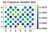
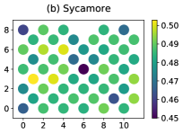
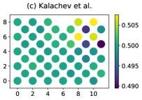
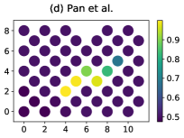
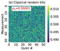
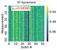
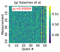
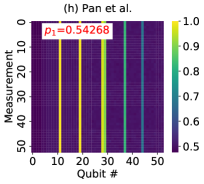
Figure 1: (First row) For 2-dimensional arrays of the Sycamore quantum processor with 53 qubits, the averages of finding outcome 1 of each qubit over one million measurements are plotted for (a) the classical random bit strings, (b) the Sycamore sample (measurement-n53-m20-s0-e0-pABCDCDAB.txt), (c) Kalachev et al. sample (samples-m20-f0-002.txt), and (d) Pan sample (sample-metropolis.txt). (Second row) The heat maps are plotted for (e) classical random bits (f) the Sycamore sample, (f) Kalachev et al.’s sample, (g) Pan et al.’s sample. The average of finding bit 1 over the sample is denoted by $p_{1}$.

II.2.3 Heat maps of bit strings.

A heat map is a good way of visualizing the statistical properties of outcomes of each qubits. The averages of outcomes at each qubit arranged in the 2-dimensional array of the Sycamore processor are plotted for the classical random bits in Fig. 1 (a), the Sycamore sample in Fig. 1 (b), the Kalachev sample in Fig. 1 (c), and the Pan et al.’s sample in Fig. 1 (d), Kalachev et al.’s sample and Pan et al.’s sample, both of which were obtained using the tensor network simulation, look like only that a random quantum circuit acts on only some parts of 53 qubits. Especially, Pan et al’s spoofing sample is quite different from the other three samples. As the animations in Supplemental Material show [44], for Pan et al’ spoofing sample, some qubits are turned always off (and turned on later).

To see the statistical difference among samples in detail, we slice a $10^{6}\times 53$ bit array, ${\cal D}=(x_{1},x_{2},\dots,x_{M})^{t}$, into $53\times 53$ square arrays $\{A^{(i)}\}$ with $i=1,\dots,L$ and $L\equiv{\rm int}(M/53)$. The heat maps of the averages of $A^{(i)}$, $(1/L)\sum_{i}A^{(i)}$, for the classical random bit sample, the Sycamore sample, the Kalachev et al.’ sample, and the Pan et al.’s sample are plotted in Figs. 1 (e), (f), (g), and (h), respectively. The heat map of the classical random bits has no stripe patterns as expected. The heat map of Pan et al. sample exhibits also the stripe patterns, but is quite different from those of the Sycamore sample of Kalachev et al.’s. It is interesting to see the heat map of Kalachev et al’s samples, Fig. 1 (f) shows stripe patterns similar to that of the Sycamore sample, Fig. 1 (e) while the former passes the NIST random number tests. One may expect that bit strings which pass the NIST random number tests would do not show any patterns. However, Kalachev et al’s samples here and Zuchongzhi samples in our previous work [25] may break a common belief on random bit or random numbers.

We count the number of outcome $1$ of a sample composed of one million bit-strings, denoted by $p_{1}$. As shown in Figs. 1 (e), (f), (g) and (h), the averages of finding outcome 1 are estimated as $p_{1}=0.50001$ for the classical random bit sample, $p_{1}=0.48360$ for the Sycamore sample, $p_{1}=0.50004$ for Kalachev et al’s sample, and $p_{1}=0.545000$ for Pan et al’s sample. Note that the averages of finding outcome 1 for Zuchongzhi samples are almost 0.5. the Sycamore samples have $p_{1}$ less than 0.5 because of the readout errors [45].

II.2.4 Marchenko-Pastur distances and Wasserstein distances

One expects that two classical processors will produce the same output or statistically similar outputs. Like that, two quantum processors implement similar quantum gates will produce similar outcomes [46]. Suppose a unitary operator $V$ of an ideal processor is approximate to a unitary operators $U$ of a real processor. The error between $U$ and $V$ is defined by $E(U,V)\equiv\max_{\ket{\psi}}||(U-V)\ket{\psi}||$. If the difference in two gates is small, then measurement statistics of $U\ket{\psi}$ is approximated by $V\ket{\psi}$. This is written as the inequality [46]

$$|p_{U}-p_{V}|\leq 2E(U,V)\,.$$ (3)

If the error $E(U,V)$ is small, the difference in probabilities between measurement outcomes, $p_{U}$ and $p_{V}$, is also small.

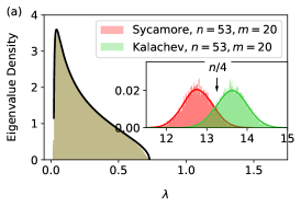
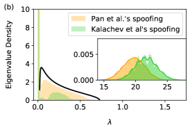
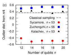
Figure 2: (a) Marchenko-Pastur distribution of eigenvalues of $(1/k)X^{t}\cdot X$, Eq. (5), for the Sycamore sample with $n=53$ and $m=20$ (red color) and for the Kalachev et al.’s sample with $n=53$ and $m=20$ (orange color). The inset shows the outlier peaks around $n/4$. (b) Marchenko-Pastur distribution of eigenvalues of $(1/k)X^{t}\cdot X$ for Pan et al.’s spoofing sample (samples-metropolis.txt) and Kalachev et al.’s spoofing sample (spoofing-m20.txt). The inset shows the outliers. (c) Marchenko-Pastur distances (outlier distances from $n/4$) as a function of the number of cycles $m$ for the Sycamore samples and Kalachev et al.’s samples with $n=53$ qubits, and for the Zuchongzhi samples with $n=56$.

If two processors, no matter processor are quantum or classical, implement the similar unitary operators for random circuit sampling, statistical distances between probabilities should be close to each other. In practice, the two probability distributions, $p_{U}(x)$ and $p_{V}(y)$, may be unknown or unavailable, but only outcomes ${\cal D}_{U}=\{x_{1},x_{2},\dots,x_{M}\}$ and ${\cal D}_{V}=\{y_{1},y_{2},\dots,y_{M}\}$ sampled from $p_{U}(x)$ and $p_{V}(y)$ are available. Thus one needs to calculate the statistical distances between two samples, ${\cal D}_{U}$ and ${\cal D}_{V}$. To this end, we employ the Marchenko-Pastur distances and the Wasserstein distances between samples.

The linear XEB, Eq. (2) is zero if bit strings are sampled from classical uniform random bits and a sample generated from a random circuit would be different. Random matrix theory, here the Marchenko-Pastur distribution of random matrices [47], could be helpful in capturing this difference. An $M\times n$ binary array ${\cal D}=(x_{1},x_{2},\dots,,x_{M})^{t}$ is sliced into into the collection of $k\times n$ rectangular random matrices $X$. Here we set $k=2n$. If all entries of $X$ are independent and identically binary random variables $\{0,1\}$, then one has the mean $\mu_{X}=1/2$ and the variance $\sigma_{X}^{2}=1/4$. We calculate the distribution of eigenvalues of square matrices $(1/k)X^{t}\cdot X$ as shown in Fig. 2. The eigenvalue distribution of $X$ is composed of the two parts: the bulk distribution is the Marchenko-Pastur distribution corresponding to random noise and the outlier represents the signal [24, 25]. The random matrices $X$ can be written as $Y=2X-J$ where $J$ of all entries 1, and $Y$ has the zero mean $\mu_{Y}=0$ and the variance $\sigma^{2}_{Y}=1$. The square random matrix $X$ can be expressed as

$$\frac{1}{k}X^{t}\cdot X=\frac{1}{4k}\left(Y^{t}\cdot Y+X^{t}\cdot J+X^{t}\cdot Z+J^{t}\cdot J\right)\,,$$ (4)

Here, the eigenvalue distribution of the first term in Eq. (4) is given by the Marchenko-Pastur distribution [47]

$$\rho(\lambda)=\frac{1}{2\pi\sigma^{2}\gamma}\frac{\sqrt{(\lambda_{+}-\lambda)(\lambda-\lambda_{-})}}{\lambda}\,,$$ (5)

where $\gamma=n/k$ is the rectangular ratio and $\lambda_{\pm}=\sigma^{2}(1\pm\sqrt{\gamma})^{2}$ are the upper and lower bounds. For $k=2n$, one has $\gamma=1/2$ and $\lambda_{+}=1+\sqrt{1/2}$. The eigenvalues of the last term $(1/4k)J^{t}\cdot J$ are 0 and $n/4$. This is the location of the outlier. We call the Marchenko-Pastur distance the distance of the peak position of the outlier of a sample from $n/4$.

Fig. 2 (a) plots the Marchenko-Pastur distribution of eigenvalues of the ensemble of $(1/2n){X^{t}\cdot X}$ for the Sycamore sample (measurement-53-m20-s0-e0-pABCDCDAB.txt) and the Kalachev et al.’s sample (samples-m20-f0-002.txt). The majority of the eigenvalues follow the Marchenko-Pastur distribution given by Eq. (5). The inset of Fig. 2 (a) shows the outliers of the distribution of eigenvalues around $n/4$, here $53/4=13.25$ for $n=53$ qubits. The distance of the peak of the outliers from $n/4$ is called the Marchenko-Pastur distance which is used to measure how a sample is deviated from classical random bit strings. Fig 2 (b) plots the Marchenko-Pastur distribution for Pan et al.’s spoofing sample (samples-metropolis.txt) and Kalachev et al. spoofing file (spoofing-m20.txt). As expected, the eigenvalue distributions of both spoofing samples are quite different from those of the Sycamore samples or those of Kalachev et al.’s samples. There is the big peak at eigenvalue zero, $\lambda=0$. Also, the outliers are far away from $n/4$.

Fig. 2 (c) plot the Marchenko-Pastur distance of samples from $n/4$ as a function of the number of cycles $m=12,14,16,18,$ and $20$. As shown in Fig. 2 (b), the Marchenko-Pastur distances of Kalachev et al.’s samples are very close to that of the classical random bit strings, approximately 0.36. The closeness of Kalachev et al.’s samples to the classical random bit strings are consistent with the fact that Kalachev et al.’s samples pass the NIST random number tests discussed above. We could not calculate the Marchenko-Pastur distribution for Pan et al.’s sample because

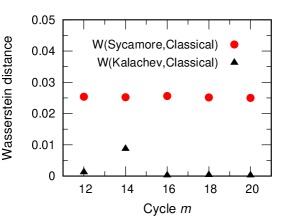
Figure 3: Wasserstein-distances of the Sycamore samples qubits with $n=53$ and the Kalachev et al.’s samples with $n=53$ from the classical random bit sample.

In order to support the analysis above using the Marchenko-Pastur distances between samples, we calculate the Wasserstein distances for samples [48]. In contrast to the Kullback-Leibler divergence, the Wasserstein distance is a metric on probability distributions. It is symmetric and satisfies the triangular inequality. The $\alpha$-Wasserstein distance between two probability distribution $p(x)$ and $q(y)$ is given by [48]

$$W(p,q)=\left(\inf_{\pi\in\Gamma(p,q)}\int_{\mathbb{R}\times\mathbb{R}}|x-y|^{\alpha}\,d\pi(x,y)\right)^{1/\alpha}\,,$$ (6)

where $\Gamma(p,q)$ is the set of joint distributions $\pi(x,y)$ whose marginals are $p(x)$ and $q(y)$. If $p(x)$ is the empirical distribution of a dataset $D_{1}=\{x_{1},x_{2},\dots,x_{M}\}$ and $q(y)$ is the empirical distribution of a dataset $D_{2}=\{y_{1},y_{2},\dots,y_{M}\}$, then $\alpha$-Wasserstein distance is written as

$$W_{\alpha}(p,q)=\left(\sum_{i=1}^{M}|x_{(i)}-y_{(i)}|^{\alpha}\right)^{1/\alpha}\,,$$ (7)

where $x_{(k)}$ denotes the order statistic of rank $k$, i.e., $k$-th smallest value in the dataset ${\cal D}_{1}$. Here, we calculate the first Wasserstein distance for the datasets of random circuit sampling using the python optimal transport library [49]. To this end, each bit string $x$ is converted to a value in range $[0,1]$ by dividing it by $1/2^{n}$. Also, we consider only 1 million bit strings. Fig. 3 plots the Wasserstein distances of samples from the classical random bit strings as a function of the number of cycles $m$. It is shown that the Wasserstein distances between Kalachev et al.’s samples and the classical random bit strings are very close. This result is consistent with the analysis with the Marchenko-Pastur distance. The Wasserstein distances of Pan et al’s spoofing sample from the classical random sample, the Sycamore sample, Kalachev et al.’s spoofing sample are about 0.0234, 0.01390, and 0.3275, respectively.

III Conclusion

In summary, we have investigated the statistical properties of bit-strings sampled from random circuits on the Sycamore quantum processor and obtained using the tensor network simulation on classical processors. We considered Kalachev et al.’s samples [17, 18, 28] and Pan et al.’s spoofing sample [19, 20, 29], and compared them with the Sycamore dataset [27] and the classical random bit strings. We found that Kalachev et al.’s samples pass the NIST random number tests while they have stripe patterns of the heat maps. The heat maps of the two spoofing samples were shown to be quite different from those of the Sycamore samples. Since some parts of bit-strings of the spoofing samples are fixed to zeros or ones, the outcomes of the spoofing samples look like that a random circuit applied only a few qubits. So one can easily distinguish them from the Sycamore samples while the linear XEB values of the spoofing samples are greater than zeros. Using the Marchenko-Pastur distribution of eigenvalues of the samples and the Wasserstein distances between the samples show that Kalachev et al.’s sample is close to classical random bit strings and the spoofing samples are far away from the classical samples or from the Sycamore samples.

Google’s 2019 experiment on random circuit sampling [9] was a landmark in quantum computing and has been much attraction as well as intense debates [50]. The tensor network simulation on quantum circuits has been proven to be effective compared the Schrödinger-Feynman simulation and could catch up with current noisy quantum processors [17, 18, 19, 20, 21]. All claims are based on two metrics: computational time and the linear XEB. While the linear XEB may serve as a good measure to verify quantum advantage, its limitation has been pointed out [22, 17, 20]. Other measures could be used to verify quantum computation for sampling [39]. For example, the random matrix analysis or the Wasserstein distances  [24, 25] would tell us other aspects of outcomes of random circuit sampling. As more results from quantum processors and advanced simulation on classical processors become available, a comparative study could deepen our understanding of quantum advantage. Our results raise a question about the claim that quantum advantage for random circuit sampling is faded by classical computers [20, 21].