Approximation by Power Series of Functions

Abstract

Derivative-matching approximations are constructed as power series built from functions. The method assumes the knowledge of special values of the Bell polynomials of the second kind, for which we refer to the literature. The presented ideas may have applications in numerical mathematics.

Introduction

Given a function $f$ and a point of expansion $x_{0}$, it is customary to say that the Taylor polynomial (TP) of degree one, two, three,… is the best linear, quadratic, cubic,… approximation of $f$ at $x_{0}$. In this sense we present here several new approximations $\mathcal{A}_{i}^{f}$ of $f$ such that

$$\frac{d^{n}}{dx^{n}}f\left(x\right)|_{x=0}=\frac{d^{n}}{dx^{n}}\mathcal{A}_{i}^{f}\left(x\right)|_{x=0},\quad n\in\mathbb{N}_{0},$$ (1)

where, without loss of generality, we assume that the expansion is done at $x_{0}=0$ (shift to an arbitrary point $x_{0}$ is achieved by shifting the argument). We denote the equality (1) by $f\approx\mathcal{A}_{i}^{f}$.

1 Power series built from functions

We build $\mathcal{A}_{i}^{f}$ as a power series of some properly chosen function $g$ following the construction from Sec. 4.1.2 of [1]. We propose

$$\mathcal{A}_{i}^{f}\left(x\right)=\sum_{n=0}^{\infty}a_{n}\left[g\left(x\right)\right]^{n}\approx f(x)\text{ with }\;g\left(0\right)=0\text{ and }g^{\prime}\left(0\right)\neq 0.$$ (2)

The existence of a non-zero derivative at zero implies $g$ can be inverted on some neighborhood of zero $x\equiv g^{-1}\left(y\right)$. We have

$$f\left[g^{-1}\left(y\right)\right]\approx\sum_{n=0}^{\infty}a_{n}y^{n},$$ (3)

i.e. the expansion coefficients $a_{n}$ are given by the power expansion coefficients of $f\left(g^{-1}\right)$

$$a_{n}=\frac{1}{n!}\frac{d^{n}}{dx^{n}}f\left(g^{-1}\left(x\right)\right)|_{x=0}.$$ (4)

This can be written in terms of the Faà di Bruno’s formula, where the Bell polynomials of the second kind $B_{n,k}$ appear

$$a_{n}=\frac{1}{n!}\sum_{k=0}^{n}d_{k}^{f}B_{n,k}(d_{1}^{g^{-1}},d_{2}^{g^{-1}},\ldots,d_{n-k+1}^{g^{-1}});\quad d_{n}^{h}\equiv\frac{d^{n}}{dx^{n}}h\left(x\right)|_{x=0}.$$ (5)

In [1] only few expansions were presented, here we systematically review the existing formulas for special values of the Bell polynomials [2, 3, 4] and propose a larger number of them.

To keep the text brief, we organize our results as a list where only the necessary information is summarized. We define

$$(-1)!! =1,\qquad 0^{0}=1,\qquad\left\langle\alpha\right\rangle_{n}=\prod_{k=0}^{n-1}\left(\alpha-k\right)\text{ //falling factorial,}$$

$$W\left(x\right) \rightarrow\text{principal branch of the Lambert W function,}$$

$$\left\llbracket\begin{array}[]{c}n\\ m\end{array}\right\rrbracket =\frac{1}{m!}\sum_{k=0}^{m}\left(-1\right)^{k}\binom{m}{k}\left(m-k\right)^{n},$$

(Stirling numbers of the second kind)

$$\left[\begin{array}[]{c}n\\ m\end{array}\right] =\sum_{j=0}^{n-m}\left(-1\right)^{j}\binom{n-1+j}{n-m+j}\binom{2n-m}{n-m-j}\left\llbracket\begin{array}[]{c}n-m+j\\ j\end{array}\right\rrbracket.$$

(Stirling numbers of the first kind)

When needed, we extend the definition of $g$ (or $g^{-1}$) to zero by its limit value

$$g(0)=\lim_{x\rightarrow 0^{(\pm)}}g\left(x\right),$$

and note it with $\doteq$. The exact version of the limit (left, right, both sides) depends on the context.

2 List of expansions

The expansion is for all cases constructed as

$$\mathcal{A}_{i}^{f}\left(x\right)=f(0)+\sum_{n=1}^{N}\frac{1}{n!}\left[\sum_{k=1}^{n}d_{k}^{f}B_{n,k}(d_{1}^{g^{-1}},d_{2}^{g^{-1}},\ldots,d_{n-k+1}^{g^{-1}})\right]\left[g\left(x\right)\right]^{n},$$ (6)

where we isolate the constant term so as to avoid ambiguities for $n=0$ (such as $0^{0}$) in the formulas which follow. We separate cases where an explicit formula for $g$ is found and those where it is not. In the first scenario we present also the formula for the Belle polynomial values, in the second situation we do this only for short formulas, for the long ones we cite the literature. The displayed constants directly appearing as arguments of the Belle polynomials $B_{n,k}(c_{1},c_{2},c_{3},\ldots)$ give the information about the derivatives of $g^{-1}$ at zero for the case in question, i.e. $c_{i}=d_{i}^{g^{-1}}$.

2.1 Formulas with explicit expression for $g$

• Logarithm-based expansion ($\mathcal{A}_{1}^{f}$)

  $$g\left(x\right) =\ln\left(x+1\right);\quad g^{-1}\left(x\right)=\exp\left(x\right)-1,$$ (7)

  $$B_{n,k}(1,1,1,\ldots)=\left\llbracket\begin{array}[]{c}n\\ k\end{array}\right\rrbracket.$$

• Exponential-based expansion ($\mathcal{A}_{2}^{f}$)

  $$g\left(x\right) =1-e^{-x};\quad g^{-1}\left(x\right)=-\ln\left(1-x\right),$$ (8)

  $$B_{n,k}(0!,1!,2!,\ldots)=\left(-1\right)^{n-k}\left[\begin{array}[]{c}n\\ k\end{array}\right].$$

• Expansion with inverse hyperbolic sine ($\mathcal{A}_{3}^{f}$)

  $$g\left(x\right) =\text{asinh}(x);\quad g^{-1}\left(x\right)=\sinh(x),$$ (9)

  $$B_{n,k}(1,0,1,0,1\ldots)=\frac{1}{2^{k}k!}\sum_{l=0}^{k}\left(-1\right)^{l}\binom{k}{l}\left(k-2l\right)^{n}.$$

• Arcus-sine-based expansion ($\mathcal{A}_{4}^{f}$)

  $$g\left(x\right) =\arcsin(x);\quad g^{-1}\left(x\right)=\sin(x),$$ (10)

  $$B_{n,k}(1,0,-1,0,1\ldots)=\frac{\left(-1\right)^{k}}{2^{k}k!}\cos\left[\frac{\left(n-k\right)\pi}{2}\right]\sum_{q=0}^{k}\left(-1\right)^{q}\binom{k}{q}\left(2q-k\right)^{n}.$$

• Expansion in powers of $\sqrt[\alpha]{x+1}-1$ ($\mathcal{A}_{5}^{f}$)

  $$g\left(x\right) =\sqrt[\alpha]{x+1}-1;\quad g^{-1}\left(x\right)=(1+x)^{\alpha}-1;\quad\alpha\in\mathbb{R}\backslash\left\{0\right\},$$ (11)

  $$B_{n,k}\left(\left\langle\alpha\right\rangle_{1},\left\langle\alpha\right\rangle_{2},\left\langle\alpha\right\rangle_{3},\ldots\right)=\frac{\left(-1\right)^{k}}{k!}\sum_{l=0}^{k}\left(-1\right)^{l}\binom{k}{l}\left\langle\alpha l\right\rangle_{n}.$$

  Notable spacial cases (polynomial and rational) happen for $\alpha=\pm 1/n$, $n\in\mathbb{N}$. For $\alpha=1$ the TP is constructed.

• Square-root-based expansion ($\mathcal{A}_{6}^{f}$)

  $$g\left(x\right) =\sqrt{2x+w^{2}}-w;\quad g^{-1}\left(x\right)=\frac{1}{2}x^{2}+wx;\quad w\in\mathbb{R}\backslash\left\{0\right\},$$ (12)

  $$B_{n,k}\left(w,1,0,0,0,\ldots\right)=\frac{1}{2^{n-k}}\frac{n!}{k!}\binom{k}{n-k}w^{2k-n}.$$

• Polynomial expansion ($\mathcal{A}_{7}^{f}$)

  $$g\left(x\right) =\frac{x^{2}+2\sqrt{\alpha}x}{\beta};\quad g^{-1}\left(x\right)=\sqrt{\alpha+\beta x}-\sqrt{\alpha};\quad\alpha,\beta\in\mathbb{R}\backslash\left\{0\right\},$$ (13)

  $$B_{n,k}\left(d_{1}^{g^{-1}},d_{2}^{g^{-1}},\ldots\right)=\left(-1\right)^{n+k}\frac{\left[2\left(n-k\right)-1\right]!!}{\alpha^{n-k/2}}\left(\frac{\beta}{2}\right)^{n}\binom{2n-k-1}{2\left(n-k\right)},$$

  where

  $$d_{n}^{g^{-1}}=\alpha^{\frac{1}{2}-n}\beta^{n}\prod_{k=1}^{n}\left(k+\frac{1}{2}-n\right).$$

• Expansion with the square root in the denominator ($\mathcal{A}_{8}^{f}$)

  $$g\left(x\right) =1-\frac{1}{\sqrt{x+1}};\quad g^{-1}\left(x\right)=\frac{1}{\left(x-1\right)^{2}}-1,$$ (14)

  $$B_{n,k}(2!,3!,4!,\ldots)=\frac{n!}{k!}\sum_{l=0}^{k}\left(-1\right)^{k-l}\binom{k}{l}\binom{n+2l-1}{n}.$$

• Expansion with fraction including square root ($\mathcal{A}_{9}^{f}$)

  $$g\left(x\right) \doteq\frac{-1+\sqrt{4x^{2}+1}}{2x};\quad g^{-1}\left(x\right)=\frac{x}{1-x^{2}},$$ (15)

  $$B_{n,k}(1!,0,3!,0,5!,0\ldots)=\frac{1+\left(-1\right)^{n+k}}{2}\frac{n!}{k!}\binom{\frac{n+k}{2}-1}{k-1}.$$

• Expansion with the Lambert function ($\mathcal{A}_{10}^{f}$)

  $$g\left(x\right) =W\left[e^{w-1}\left(w+x-1\right)\right]+1-w,\quad w\in\mathbb{R}\backslash\left\{0\right\},$$ (16)

  $$g^{-1}\left(x\right) =\left(w+x-1\right)e^{x}+1-w,$$

  $$B_{n,k}(w,w+1,w+2,\ldots) =$$

  $$\qquad=k^{n-k}\binom{n}{k}\sum_{l=0}^{k}\binom{k}{l} \left[\sum_{q=0}^{n-k}\frac{\left(-1\right)^{q}}{k^{q}}\binom{n-k}{q}\frac{\left\llbracket\begin{array}[]{c}l+q\\ l\end{array}\right\rrbracket}{\binom{l+q}{l}}\right]\left(w-1\right)^{l}.$$

• Second expansion with the Lambert function ($\mathcal{A}_{11}^{f}$)

  $$g\left(x\right) =\frac{W\left[-e^{-(x+1)}(x+1)\right]}{x+1}+1;\quad g^{-1}\left(x\right)\doteq-\frac{\ln\left(1-x\right)}{x}-1,$$ (17)

  $$B_{n,k}\left(\frac{1!}{2},\frac{2!}{3},\frac{3!}{4},\ldots\right)=\frac{(-1)^{n-k}}{k!}\sum_{m=0}^{k}\left(-1\right)^{m}\binom{k}{m}\frac{\left[\begin{array}[]{c}n+m\\ m\end{array}\right]}{\binom{n+m}{m}}.$$

  As readily seen form the argument of the function $W$(which is defined from $-1/e$ to $\infty$), this approximation is valid in the right neighborhood of zero.

• Third expansion with the Lambert function ($\mathcal{A}_{12}^{f}$)

  $$g\left(x\right) =-\frac{W\left(-\frac{\exp\left(-\frac{1}{1+x}\right)}{1+x}\right)+xW\left(-\frac{\exp\left(-\frac{1}{1+x}\right)}{1+x}\right)+1}{1+x},$$ (18)

  $$g^{-1}\left(x\right) \doteq\frac{e^{x}-1}{x}-1,$$

  $$B_{n,k}\left(\frac{1}{2},\frac{1}{3},\frac{1}{4},\ldots\right)=\frac{n!}{\left(n+k\right)!}\sum_{l=0}^{k}\left(-1\right)^{k-l}\binom{n+k}{k-l}\left\llbracket\begin{array}[]{c}n+l\\ l\end{array}\right\rrbracket.$$

  As readily seen form the argument of the function $W$, this approximation is valid in the left neighborhood of zero.

• Powers of sine ($\mathcal{A}_{13}^{f}$)

  $$g\left(x\right) =\sin\left(x\right),$$ (19)

  $$g^{-1}\left(x\right) =\arcsin\left(x\right),$$

  $$B_{n,k}\left(1,0,1,0,9,0,225,0,\ldots,\left[\left(n-k-3\right)!!\right]^{2},0,\left[\left(n-k-1\right)!!\right]^{2}\right)=$$

  $$=\delta_{\left(n-k\right)\%2,0}\left(-1\right)^{\frac{n-k}{2}}2^{n-k}\sum_{l=0}^{n-k}\binom{k+l-1}{k-1}\left[\begin{array}[]{c}n-1\\ k+l-1\end{array}\right]\left(\frac{n-2}{2}\right)^{l},$$

  where $\delta$ is the Kronecker delta and $\%$ is the modulo operation. This expansion has large similarities with [5] and represents Fourier series whose standard form can be get by applying trigonometric power formulas to $\left[\sin\left(x\right)\right]^{n}$ terms.

2.2 Formulas without explicit expression for $g$

With the function $g^{-1}$ known, one can use numerical or approximation methods to get $g$ in the proximity of zero.

• Case one
  

  $$g^{-1}\left(x\right)=(w-1+e^{x})x;\quad w\neq 0,$$ (20)

  $$B_{n,k}(w,2,3,4,\ldots)=\binom{n}{k}\sum_{r=0}^{k}\binom{k}{r}\left(k-r\right)^{n-k}\left(w-1\right)^{r}.$$

• Case two
  

  $$g^{-1}(x)=e^{x}(x-2)-x+2,$$ (21)

  $$B_{n,k}(-2,0,1,2,3,\ldots) =\sum_{r=0}^{n}r!\binom{n}{r}\binom{k}{r}\left(-2\right)^{k-r}\left\llbracket\begin{array}[]{c}n-r\\ k\end{array}\right\rrbracket.$$

• Case three
  

  $$g^{-1}(x)=\left(2e^{x}-x^{2}-2x-2\right)/\left(2x^{2}\right).$$ (22)

  The formula for $B_{n,k}(\frac{1}{2.3},\frac{1}{3.4},\ldots)$ is shown in Eq. (2.1) of [2].

• Case four
  

  $$g^{-1}(x)=\left(6xe^{x}-12e^{x}-x^{3}+6x+12\right)/\left(6x^{3}\right).$$ (23)

  The formula for $B_{n,k}(\frac{1}{3.4},\frac{1}{4.5},\ldots)$ is shown in Theorem 2.7 of [2].

• Case five
  

  $$g^{-1}(x)=\alpha+(\alpha+a_{1}-1)x+\frac{1}{2}(\alpha+a_{2}-2)x^{2}+(x-\alpha)e^{x};\quad a_{1}\neq 0.$$ (24)

  The formula for $B_{n,k}(a_{1},a_{2},3-\alpha,4-\alpha,5-\alpha,\ldots)$ is shown in Eq. (3.1) of [2]. The function $g$ can be expressed in terms of the Lambert $W$ for $a_{1}=1-\alpha$ and $a_{2}=2-\alpha$, which however corresponds to Eq. (16) from the previous section.

• Case six
  

  $$g^{-1}(x)\doteq-\frac{\left[\arccos\left(x+1\right)\right]^{2}}{2x}-1.$$ (25)

  The formula for $B_{n,k}\left(-\frac{2}{12},\frac{4}{45},-\frac{6}{70},\ldots,2\frac{(2n-2k+2)!!}{(2n-2k+4)!}Q(2,2n-2k+2)\right)$ together with the definition of $Q$ is shown in Eqs. (5.1) and (2.3) of [3].

3 Discussion and remarks

Plots

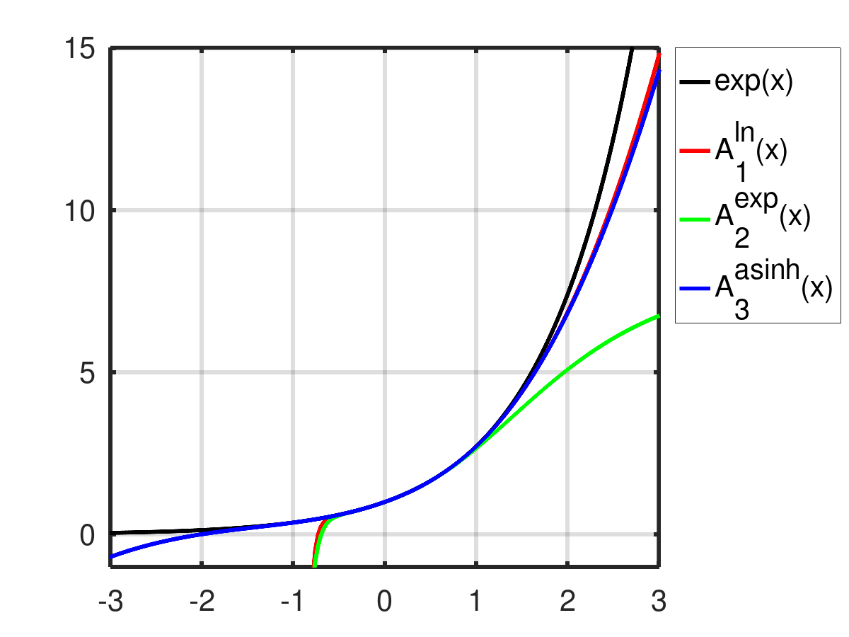
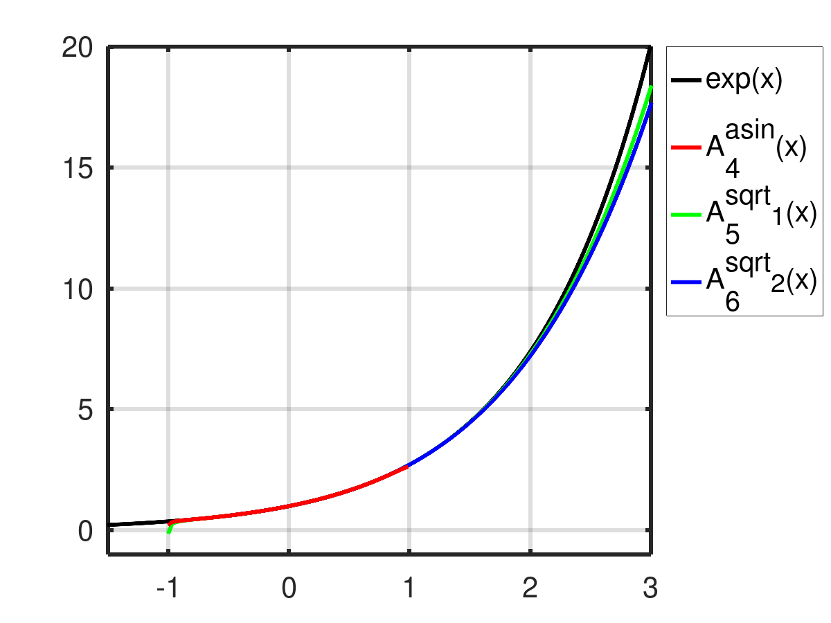
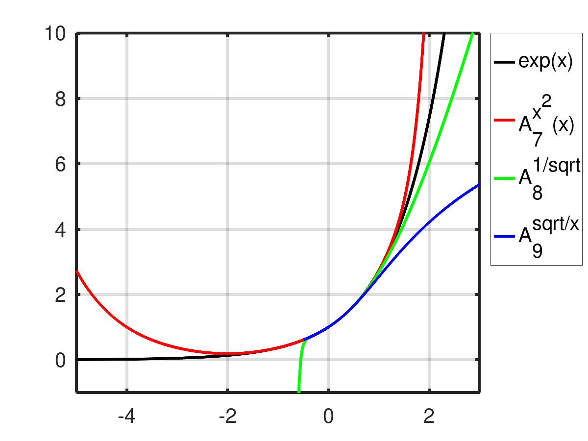
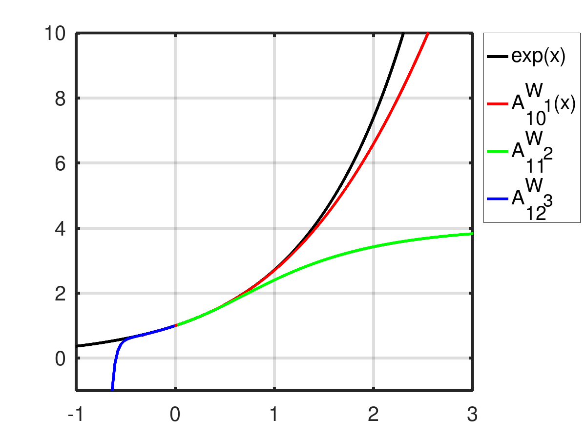
Figure 2: The $\exp\left(x\right)$ function approximated by series (6) with 8 terms and with various $g$ from Sec. 2.1.

In Figs. (2)-(5), situated at the end of this text, we provide plots where four elementary functions $\exp\left(x\right)$, $\sin\left(x\right)$, $x^{2}$ and $\ln\left(x+1\right)$ are approximated with expansions based on Eqs. (7)-(19), the value and first seven derivatives are matched. For the sake of comparison we also include the TP. The numbering subscript of approximations $\text{A}_{\text{no.}}$ in the legend respects the order in which the $g$ functions are presented in the Sec. 2.1 and the superscript attempts to mimic the function form of $g$ so as to remind the reader about it. The parametric expressions (11),(12),(13) and (16) are show with parameters $\alpha=2$, $w=1$, $\left(\alpha=4,\beta=3\right)$ and $w=1$, respectively. Some lines in the graphs are overlaid, the reason is mostly the fact that the approximation is exact.

Convergence

Convergence properties can be easily addressed since the substitution as expressed by the Eq. (3) does not influence the point-wise behavior. So, considering

$$f\left(x\right)=f\left[g^{-1}\left(y\right)\right]\approx\sum_{n=0}^{\infty}a_{n}y^{n},$$

one applies the standard convergence criteria known from the usual power series to the coefficient sequence $\{a_{n}\}$ and determines the radius of convergence $R$ for the variable $y$

$$\left|y\right|<R\Rightarrow\sum_{n=0}^{\infty}a_{n}y^{n}\text{ converges}.$$

Then for all $x\in U$, $U=\{x\in\mathbb{R}:\left|g\left(x\right)\right|<R\}$, the series $\sum_{n=0}^{\infty}a_{n}\left[g\left(x\right)\right]^{n}$converges.

The convergence to the approximated function can also be treated in this way, for simplicity we assume that we work on an interval $\mathcal{I}$ containing zero where $g$ can be inverted. Writing an equality which includes the reminder term

$$f\left[g^{-1}\left(y\right)\right]=\sum_{n=0}^{M}a_{n}y^{n}+R_{M}\left(y\right),$$

one can apply the standard criteria known from the Taylor series to see whether, in a point-wise way, the reminder vanishes with $M\rightarrow\infty$ at some $y_{0}$. If $W$ is the set of all points such that

$$y\in W\Rightarrow\sum_{n=0}^{\infty}a_{n}y^{n}=f\left[g^{-1}\left(y\right)\right],$$

then for all $x\in\mathbb{\mathcal{I}}$ such that $g\left(x\right)\in W$ one has $f\left(x\right)=\sum_{n=0}^{\infty}a_{n}\left[g\left(x\right)\right]^{n}.$

The most difficult part is presumably the application of the standard criteria to $\{a_{n}\}$, since the expression (5) is rather complicated (may contain several nested sums).

The convergence criteria can be in a straightforward way extended to the complex analysis.

Polynomial approximations

One observes that pure polynomial approximations are in the list: the parametric expression (11) with $\alpha=1/k,\>k\in\mathbb{N}^{+}$ and the expression (13). It is interesting to realize, that these expansions in general do not exactly approximate polynomials with the same number of terms. Since the polynomial coefficients are in the one-to-one correspondence with the derivatives $d_{k}^{f}$, the two approximations contain the TP as their lower terms up to $x^{N}$. In addition, they also contain higher order terms which imply the deviations from the approximated function if the latter is a polynomial of the degree $N$.

Further, expansions (11) and (12) with shifted arguments $\mathcal{A}_{5}^{f}\left(x-1\right)$ and $\mathcal{A}_{6}^{f}\left(x-\omega^{2}/2\right)$ allow to build expressions where the integer and/or fractional powers of $x$ appear. They represent fractional order polynomials which have already been introduced in the literature and in a special case are written as

$$F\left(x\right)=\sum_{n=0}^{N}c_{k}\left(x^{\alpha}\right)^{n},\quad\alpha>0,$$ (26)

see e.g. Eq. (4) in [6] or Eq. (11) in [7].

Applications

The applications may result from better approximation properties than what is provided by the TPs. This however depends on the approximated function, yet some claims are evident, e.g. there are cases where an approximation proposed here converges beyond the radius of the convergence of the Taylor series. Indeed, the function $\ln\left(x+1\right)$, when expanded at zero, can be approximated by the TPs on the interval $\left(-1,1\right)$ only. By (7) it is approximated on the whole definition interval exactly and with one term.

To be more fair, we compare the expansion in powers of $g$ from Eq. (14) with the TP inside its radius of convergence, i.e. we numerically investigate the approximation of $\ln\left(x+1\right)$ at $x=0.5$. We define $\varDelta_{f}=\left|\ln\left(1.5\right)-f(1.5)\right|$ and we get ($N$ is the number of terms in the series, see (6))

$N$	3	7	10	20
$\varDelta_{\mathcal{A}_{8}^{f}}\approx$	$6.65\times 10^{-4}$	$3.84\times 10^{-7}$	$1.74\times 10^{-9}$	$3.33\times 10^{-16}$
$\varDelta_{TP}\approx$	$1.12\times 10^{-2}$	$3.38\times 10^{-4}$	$3.05\times 10^{-5}$	$1.53\times 10^{-8}$

The first few cutoff series for both cases indicate a significant difference in the rate of convergence in favor of the expansion $\mathcal{A}_{8}^{f}$.

An important disadvantage for an eventual implementation of the series (7)-(19) on a computer might be the time necessary for computing $g\left(x\right)$ from $x$. To speed up the evaluation of (2) the Horner’s method is to be used. More importantly, a couple of expansions from Sec. 2.1 are based on the square root, which is for several common architectures implemented as a basic arithmetic operation included into the instruction set of the processor (often labeled fsqrt, see [8] for x86, [9] for ARM ). This means it can be evaluated very rapidly which, in combination with possible better convergence properties, can be a reason for implementing new algorithms to compute values of some functions.

In this spirit, one potentially interesting application is the computation of the $m$th root, which is (usually) not a basic instruction of a processor. Our preliminary tests indicate that $\sqrt[m]{x+1}$ can be for $-1<x$, $1<m\in\mathbb{R}$ computed by the series based on the expansion in powers of (11), $\alpha=2$,

• with a significantly higher rate of convergence than have the Taylor series (within its convergence domain) and

• on a significantly larger interval (i.e. beyond its convergence domain).

Such behavior was observed for all $1<M$ we tested. An example with the fifth root is shown in Fig. 1. Further investigations need to be done to confirm our claims on a more rigorous basis.

Figure 1: The function $\sqrt[5]{x+1}$ approximated by the series $\mathcal{A}_{5}$ built from the powers of $\left[\sqrt{x+1}-1\right]$ and by the TP, in both cases with 8 terms.

4 Summary, conclusion, outlook

In this text we presented a number of presumably new expansions built as powers series constructed from functions, we addressed and clarified the question of their point-wise convergence and mentioned some advantages they may have in comparison with the Taylor polynomials. These advantages can represent the reason for their application potential in numerical evaluation of some functions, the issue however requires more detailed investigation in the future.

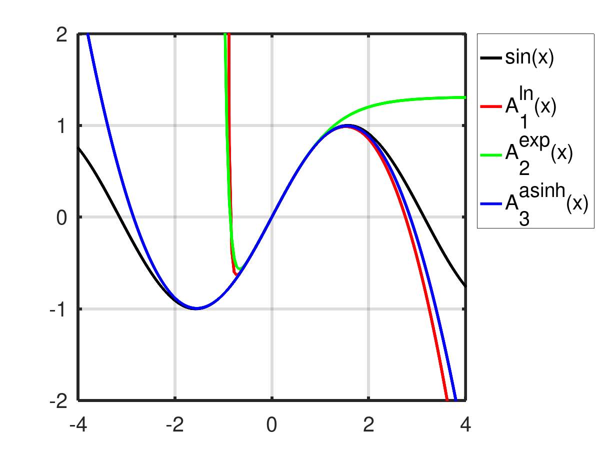
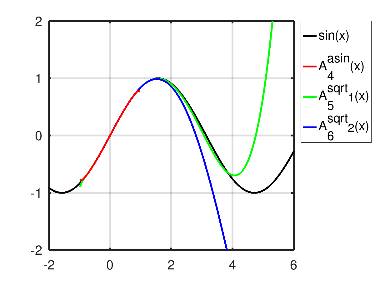
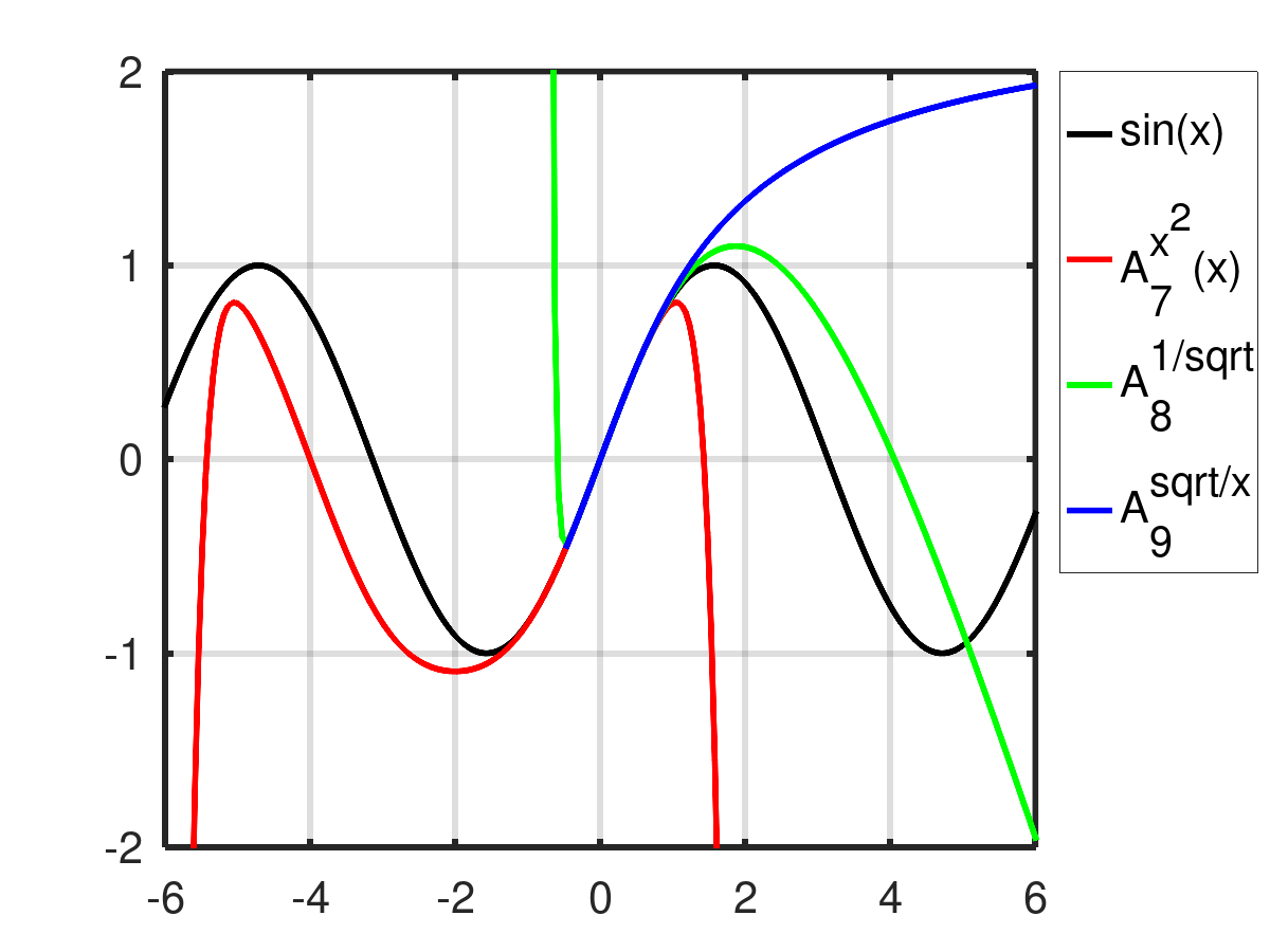
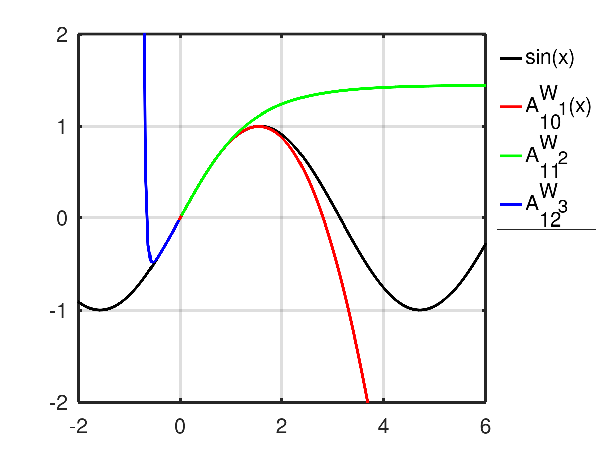
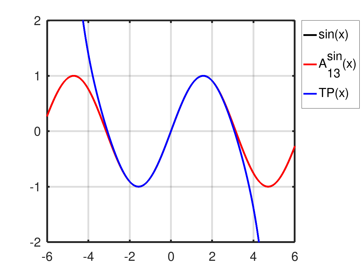
Figure 3: The $\sin\left(x\right)$ function approximated by series (6) with 8 terms and with various $g$ from Sec. 2.1.

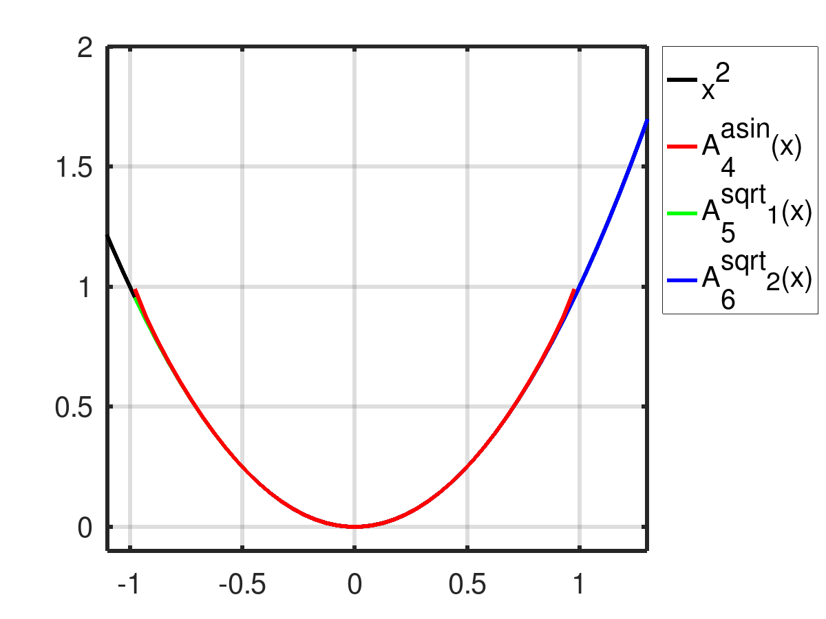
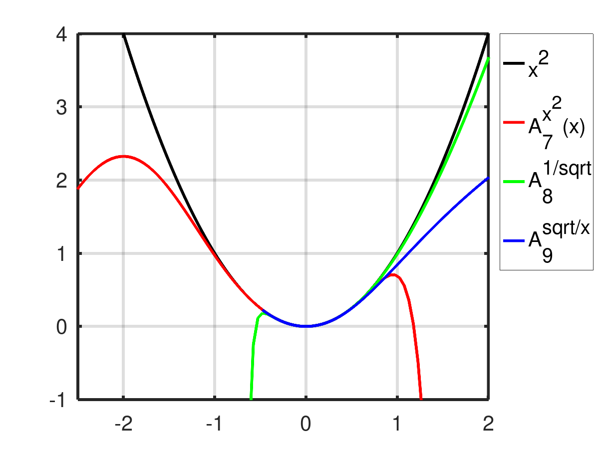
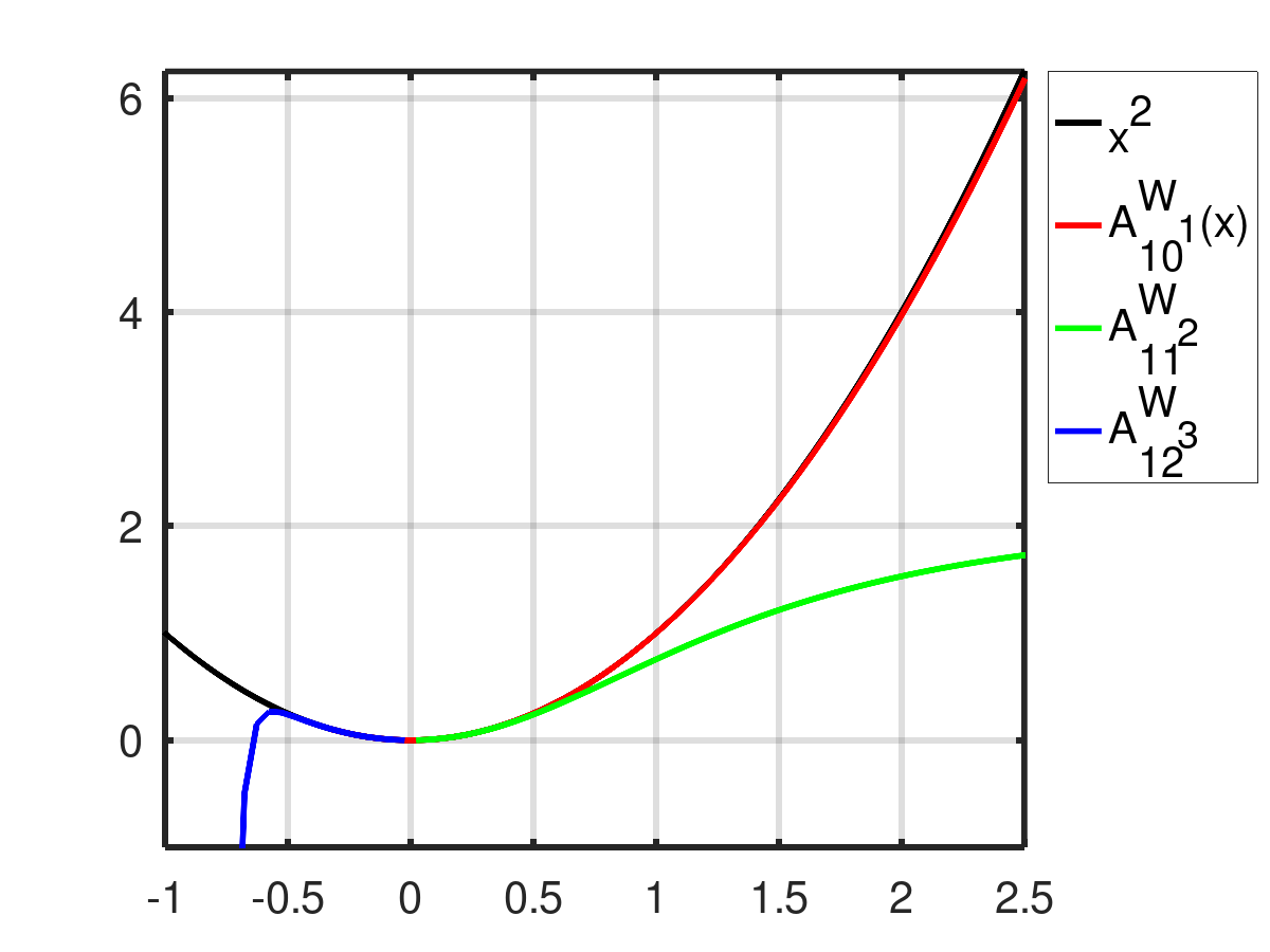
Figure 4: The $x^{2}$ function approximated by series (6) with 8 terms and with various $g$ from Sec. 2.1.

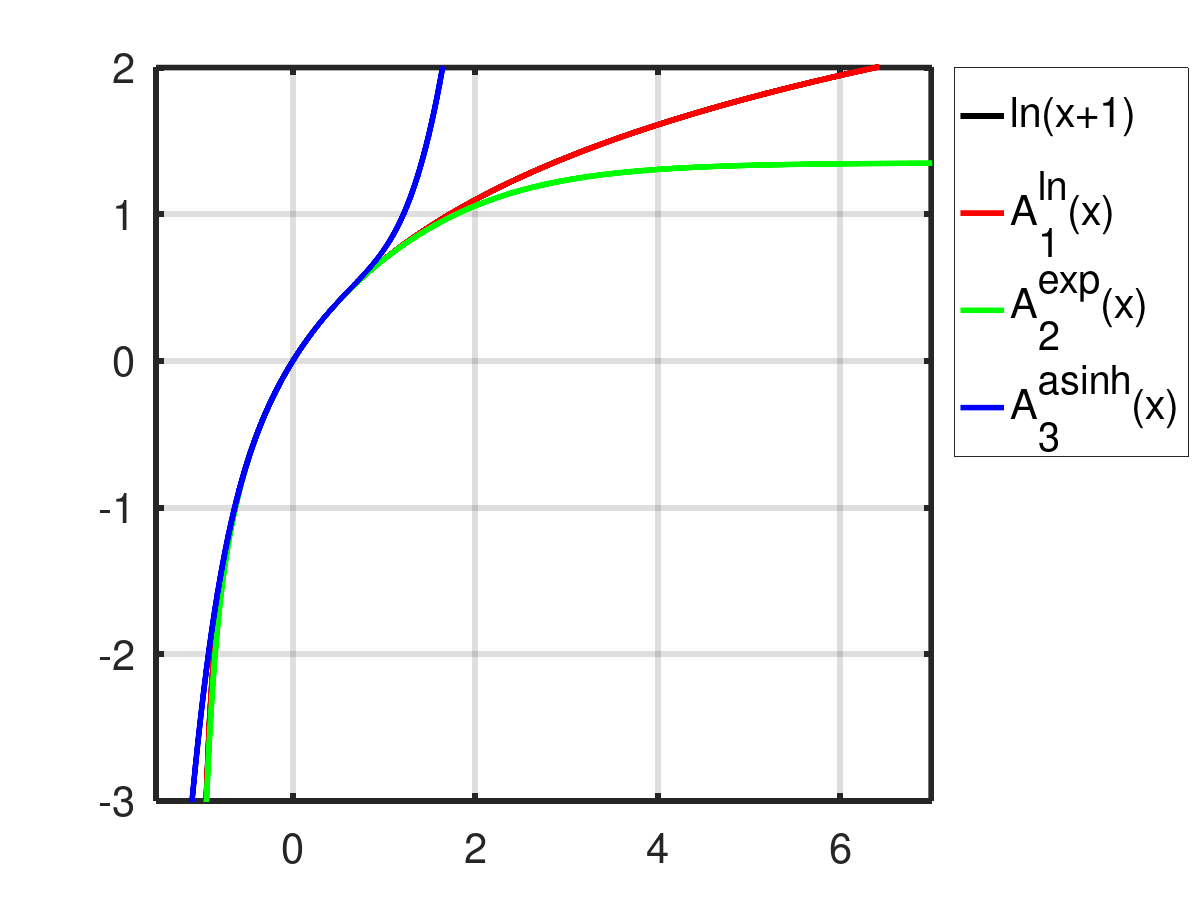
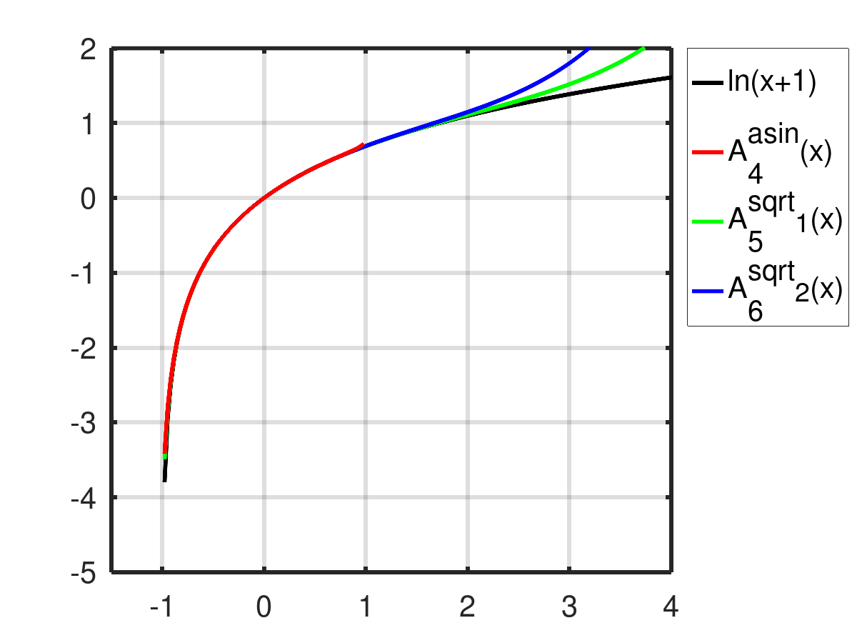
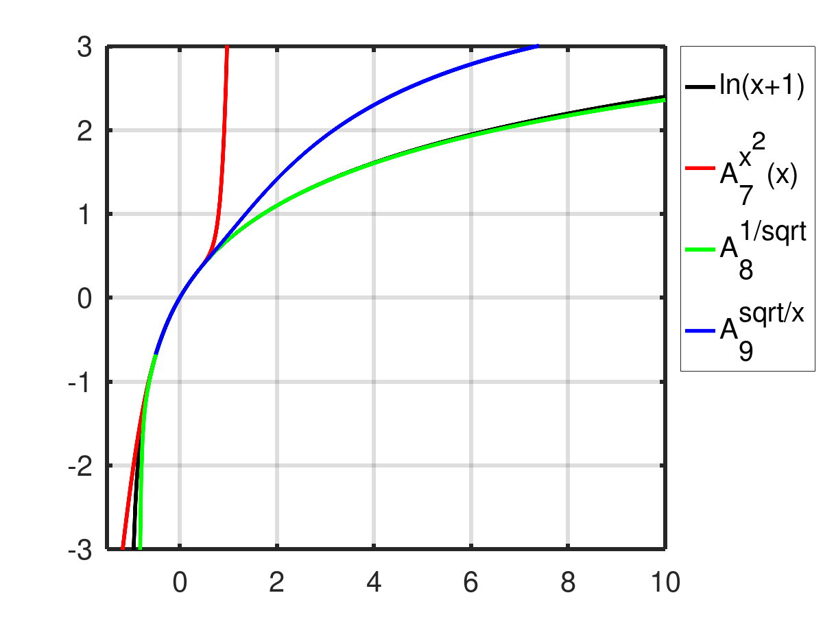
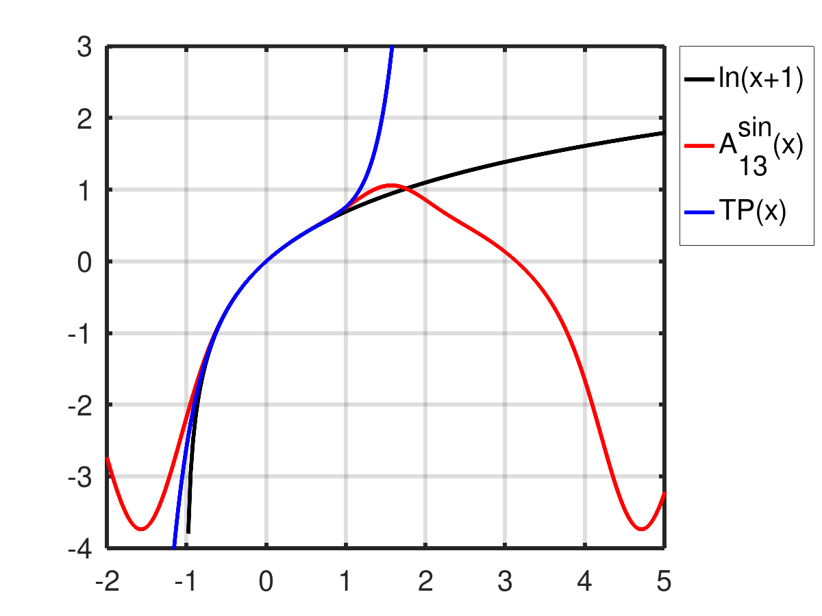
Figure 5: The $\ln\left(x+1\right)$ function approximated by series (6) with 8 terms and with various $g$ from Sec. 2.1.

References

• [1] LiptajΒ A. General approach to function approximation. β€”β€…2022. β€”β€…https://arxiv.org/abs/2201.07983.
• [2] Special values of the bell polynomials of the second kind for some sequences and functionsΒ / FengΒ Qi, Da-WeiΒ Niu, DongkyuΒ Lim, Yong-HongΒ YaoΒ // Journal of Mathematical Analysis and Applications. β€”β€…2020. β€”β€…Vol. 491, no.Β 2. β€”β€…P.Β 124382. β€”β€…Access mode: https://www.sciencedirect.com/science/article/pii/S0022247X20305448.
• [3] QiΒ F. Taylor’s series expansions for real powers of two functions containing squares of inverse cosine function, closed-form formula for specific partial bell polynomials, and series representations for real powers of piΒ // Demonstratio Mathematica. β€”β€…2022. β€”β€…Vol.Β 55, no.Β 1. β€”β€…P.Β 710–736. β€”β€…Access mode: https://doi.org/10.1515/dema-2022-0157.
• [4] QiΒ F. Explicit formulas for partial bell polynomials, maclaurin’s series expansions of real powers of inverse (hyperbolic) cosine and sine, and series representations of powers of pi. β€”β€…2021. β€”β€…10. β€”β€…https://doi.org/10.21203/rs.3.rs-959177/v3.
• [5] Central factorial numbers; their main properties and some applications.Β / P.Β L.Β Butzer, K.Β Schmidt, E.L.Β Stark, L.Β VogtΒ // Numerical Functional Analysis and Optimization. β€”β€…1989. β€”β€…Vol.Β 10, no. 5-6. β€”β€…P.Β 419–488. β€”β€…Access mode: https://doi.org/10.1080/01630568908816313.
• [6] Routh table test for stability of commensurate fractional degree polynomials and their commensurate fractional order systemsΒ / Sheng-GuoΒ Wang, ShuilianΒ Liang, LiangΒ Ma, KaiΒ xiangΒ PengΒ // Control Theory and Technology. β€”β€…2019. β€”β€…Vol.Β 17. β€”β€…P.Β 297–306.
• [7] MikolajΒ B. Stability analysis of linear continuous-time fractional systems of commensurate orderΒ // Journal of Automation, Mobile Robotics & Intelligent Systems. β€”β€…2009. β€”β€…Vol.Β 3, no.Β 1. β€”β€…P.Β 12–17.
• [8] Intel CorporationⓇ. Intel 64 and ia-32 architectures software developer’s manual combined, volumes:1, 2a, 2b, 2c, 2d, 3a, 3b, 3c, 3d and 4. β€”β€…2022. β€”β€…April. β€”β€…Access mode: https://software.intel.com/en-us/download/intel-64-and-ia-32-architectures-sdm-combined-volumes-1-2a-2b-2c-2d-3a-3b-3c-3d-and-4.
• [9] Arm Limited. Armβ“‘ compiler, version 6.6, armasm user guide. β€”β€…2020. β€”β€…Access mode: https://developer.arm.com/documentation/dui0801/latest/.
Refer to caption
Refer to caption
Refer to caption
Refer to caption
Refer to caption