Lempel-Ziv Networks

Abstract

Sequence processing has long been a central area of machine learning research. Recurrent neural nets have been successful in processing sequences for a number of tasks; however, they are known to be both ineffective and computationally expensive when applied to very long sequences. Compression-based methods have demonstrated more robustness when processing such sequences — in particular, an approach pairing the Lempel-Ziv Jaccard Distance (LZJD) with the k-Nearest Neighbor algorithm has shown promise on long sequence problems (up to $T=200,000,000$ steps) involving malware classification. Unfortunately, use of LZJD is limited to discrete domains. To extend the benefits of LZJD to a continuous domain, we investigate the effectiveness of a deep-learning analog of the algorithm, the Lempel-Ziv Network. While we achieve successful proof of concept, we are unable to improve meaningfully on the performance of a standard LSTM across a variety of datasets and sequence processing tasks. In addition to presenting this negative result, our work highlights the problem of sub-par baseline tuning in newer research areas.

1 Introduction

Sequence processing has been an important focus of the machine learning community for decades. Due to the ubiquity of sequential data, there is a need for effective algorithms to process this data for a diverse set of tasks, including classification and time series analysis. Recurrent architectures such as long short-term memory (LSTM) [1] have been successful in processing sequences for a number of such tasks in recent years [2]. A known issue of recurrent networks, however, is that they tend to be both ineffective [3] and computationally expensive [4] when applied to very long sequences.These challenges have hindered efforts to learn long-term dependencies over sequential data with recurrent neural nets (RNNs).

Compression-based methods have demonstrated more robustness in tackling the issues associated with long sequences. The Lempel-Ziv Jaccard Distance (LZJD)  [5, 6, 7, 8] takes the Lempel-Ziv compression of sequences before applying the Jaccard distance to the compressions. An approach pairing LZJD with the k-Nearest Neighbor algorithm has been shown to be both more accurate and orders of magnitude faster than previous techniques for malware classification from byte sequences. However, LZJD is limited by the fact that it is only applicable in a discrete domain; moreover LZJD is unable to learn about or exploit the existence of similar compressions since it recognizes only exact matches. This is not ideal for use in areas such as malware classification, where the underlying data is continually evolving.

We explore the effectiveness of a deep-learning analog of LZJD, the Lempel-Ziv Network, at extending LZJD’s benefits to the continuous domain. Despite establishing successful proof of concept, we fail to consistently improve on the performance of a traditional LSTM over a collection of datasets and sequence processing tasks.

The rest of the paper is organized as follows. In Section 2, we review LZ compression and various types of associative memories. In Section 3, the novel Lempel-Ziv based recurrent layer is delineated. Experimental details and results are presented in Section 4. Finally, we conclude in Section 5.

2 Background

LZ compression

Table 1: LZ compression on two sequences.

Sequence	Compression
aabbaba	{a, ab, b, aba}
aabbba	{a, ab, b, ba}

Lempel-Ziv Jaccard Distance (LZJD) [5] uses Lempel-Ziv (LZ) compression to condense long sequences into a compact representation consisting of a set of unique subsequences. LZ compression works by keeping an external memory that store unique subsequences of the input sequence. To determine which subsequences are placed into the external memory, we traverse the input sequence with a sliding window. If the subsequence currently selected by the sliding window is already stored in the external memory, then we increment the “end” index of the window and keep the “start” index fixed, increasing the size of our window until the subsequence it identifies is not present in the external memory. Once such a sequence is found, we insert it into the external memory and move the “start” index of our sliding window to the current “end” index. We repeat this process to locate and insert successive unique subsequences into the external memory until we have covered the length of the input sequence.

This explication of LZ compression also reveals some of its weaknesses. Let $A,B,C$ be subsequences present in an external memory arising from LZ compression of a sequence. Let $A=\{1.29,7.89,0.11\}$, $B=\{1.28,7.91,0.10\}$, and $C=\{5.01,2.63,2.17\}$. It is clear that $A$ and $B$ are very similar to each other, and both are substantially different from $C$. Yet the LZ compression algorithm is unable to express this nuance and treats all three subsequences as being equally dissimilar, and so we end up with two nearly identical subsequences, $A$ and $B$, in our external memory. We hope that by combining the insights of LZJD with the functionality of an RNN, we can give LZ compression the flexibility to handle similar subsequences while maintaining its effectiveness as a tool for finding compact representations of long sequences.

Associative memories

We require an associative memory to perform two essential functions - we must be able to insert new items into the memory, and we must be able to query the memory for information about items it already contains. This enables an associative memory to mimic the function of LZJD’s external memory. By first querying the memory for information about prospective inputs, we can be sure to input only items (i.e. subsequences or their representations) that have not been previously inserted. Here we review the three types of associative memories with which we experimented in our LZ Layer.

Hopfield Networks [9] are among the best known associative memories. Designed to store and retrieve patterns, in response to a query $q$ Hopfield networks will return the pattern in memory most similar to $q$, or an average of similar patterns. In [10], Ramsauer et al. develop a modern Hopfield network for continuous states, with exponential storage capacity. Because patterns can be retrieved from memory in one update step, this Hopfield network is ideal for use in deep learning architectures. We utilize a static version of their Hopfield layer to perform the insert and query functions of associative memory.

Vector Symbolic Architectures (VSA) use high-dimensional vectors to imitate symbolic processing. VSAs are typically equipped with three crucial operations - a bundling operation, a binding operation, and an unbinding operation [11]. The bundling operation takes in two input vectors and outputs a third vector similar to both inputs, and is denoted by a simple addition sign. The binding operation $\mathfrak{B}$ is used to pair two vectors together, while the unbinding operation $\mathfrak{B}^{+}$ undoes this pairing. For example, by assigning concepts such as “Age” and values such as “30” to high-dimensional vectors, we could set $\textrm{John}=\mathfrak{B}(\textrm{Age},30).$ Then, using the unbinding function, we could perform a lookup, resulting in $\mathfrak{B}^{+}(\textrm{John},\textrm{Age})=30.$ By combining binding and bundling, we can create more complex representations, such as $\textrm{Jane}=\mathfrak{B}(\textrm{Age},25)+\mathfrak{B}(\textrm{Weight},120).$ However, the accuracy of the unbinding operation decreases as the number of terms bundled together increases. Maximizing this accuracy as bundle size increases is a key consideration in the choice of binding operation.

With a few additional specifications, a VSA can act as an associative memory. First, we fix a “tag” vector. Then, we bind every vector we want to insert into the associative memory to the tag vector. Our memory then becomes the bundling of all the (vector, tag) pairs. To add a new vector $v$ to the memory, we simply bundle again: $\textrm{memory}_{new}=\textrm{memory}_{old}+\mathfrak{B}(v,\textrm{tag}).$ To query the memory for a vector $q$, we compute $\mathfrak{B}^{+}(\textrm{memory},q)=\widehat{\textrm{tag}}.$ If $\widehat{\textrm{tag}}\approx\textrm{tag}$, we conclude that $q$ is stored in the associative memory. On the contrary, if $\widehat{\textrm{tag}}\not\approx\textrm{tag}$, we can assume $q$ is not in the associative memory.

In this paper, we construct associative memories using a VSA. For the bundling operation, we use simple element-wise addition. For the binding and unbinding operations, we experimented with the two different paradigms discussed in the remainder of this section.

Vector-Derived Transformation Binding (VTB) defines the binding operation $\mathfrak{B}$ as follows: for $d$ a perfect square, $d^{\prime}=d^{1/2}$, we have $\mathfrak{B}:\mathbb{R}^{d}\times\mathbb{R}^{d}\rightarrow\mathbb{R}^{d}$ where $\mathfrak{B}(x,y)=V_{y}x=\begin{bmatrix}V_{y}^{\prime}&0\\ 0&\ddots\end{bmatrix}x$ and Equation 1.

$$V_{y}^{\prime}=d^{1/4}\begin{bmatrix}y_{1}&y_{2}&\cdots&y_{d^{\prime}}\\ y_{1+d^{\prime}}&y_{2+d^{\prime}}&\cdots&y_{2d^{\prime}}\\ \vdots&\vdots&\ddots&\vdots\\ y_{1+(d-d^{\prime})}&y_{2+(d-d^{\prime})}&\cdots&y_{d}\end{bmatrix}$$ (1)

The unbinding operation, the approximate inverse of $\mathfrak{B}$, is specified by $\mathfrak{B}^{+}(x,y)=V_{y}^{\top}x$. In [12], Gosmann and Eliasmith found VTB to be an improvement over traditional binding operations such as circular convolution, as the associated unbinding operation retained a higher accuracy even when many terms were bound together. Additionally, with VTB, increased bindings had less effect on the vector norm, making VTB more suited for use in neural networks.

Holographic Reduced Representation (HRR) provides an alternative way of implementing symbolic AI. Our HRR associative memory works very similarly to its VTB counterpart - only the binding operation is changed.

HRR was first introduced by in [13]. Circular convolution and fast Fourier transforms were used to define a binding operation $\mathrel{\leavevmode\hbox to7.9pt{\vbox to7.9pt{\text{[drawing]}}}}$, where $s=a\mathrel{\leavevmode\hbox to7.9pt{\vbox to7.9pt{\text{[drawing]}}}}b=\mathcal{F}^{-1}(\mathcal{F}(a)\odot\mathcal{F}(b)).$ By defining an identity function $\mathcal{F}(a^{+})\mathcal{F}(a)=1$, an inverse $a^{+}$ for $a$ is established, where $a^{+}~{}=~{}\mathcal{F}^{-1}\Big{(}\frac{1}{\mathcal{F}(a)}\Big{)}.$ Then, unbinding proceeds as follows: $s\mathrel{\leavevmode\hbox to7.9pt{\vbox to7.9pt{\text{[drawing]}}}}a^{+}\approx b.$

This HRR, however, has some considerable limitations. First, the inverse $a^{+}$ is numerically unstable, necessitating the use of a pseudo-inverse, differing by the reciprocal of the complex magnitude, in its place. Additionally, once more than ten bound pairs are bundled together, the accuracy of the unbinding operation, used for querying in the context of associative memories, is severely diminished. These concerns are mitigated in work done by [14, 15]; [14] defines a new complex unit magnitude projection which, when applied to each input of the binding operation before binding takes place, allows for accurate unbinding with up to 100$\times$ more bound vectors. Furthermore, by ensuring that all the vectors used in the HRR are unitary, the projection guarantees that the true inverse is equivalent to the numerically stable and computationally cheaper pseudo-inverse, eliminating one source of error and providing major speed-ups during implementation. We make use of this improved HRR in building our HRR Associative Memory.

3 The Lempel-Ziv Layer

Figure 1: Diagram of a Lempel-Ziv layer.

The LZ layer (see Figure 1) begins with a standard RNN Cell, which takes in the hidden state from the previous time step ($h_{t-1}$) and the input for the current time step ($x_{t}$) and outputs a new preliminary hidden state ($\hat{h}_{t}$). In a traditional RNN, we might stop here, and just consider $\hat{h}_{t}$ to be $h_{t}$, the hidden state which is passed along as input when the next item in the sequence is processed by the RNN. However, in the LZ layer, we want to perform the LZ digest-creating behavior on this preliminary hidden state $\hat{h}_{t}$, as the hidden state is the neural representation of the subsequence of data that the traditional LZ compression algorithm would analyze.

Thus, we query the associative memory to ask if we have seen $\hat{h}_{t}$ before. The query returns a reconstructed vector $\hat{r}$, which we compare to a vector $r$ — the tag vector if using a VTB or HRR associative memory, or $\hat{h}_{t}$ itself if using a Hopfield associative memory. The closer $\hat{r}$ is to $r$, the more similar $\hat{h}_{t}$ is to something already stored in memory. We pass $\hat{r}$ and $r$ into a learnable bilinear layer, combined with a sigmoid activation function and a Bernoulli layer, to determine if $\hat{h}_{t}$ is sufficiently dissimilar to anything we have seen before, i.e., if $\hat{r}$ is sufficiently far from $r$, to insert $\hat{h}_{t}$ into the associative memory as a new value. We refer to this bilinear-sigmoid-Bernoulli combination as a novelty score, and it returns $p=1$ if it judges $\hat{h}_{t}$ to be new enough to insert, and $p=0$ otherwise.  Because the novelty score is learnable, we theorize that it will allow our LZ Layer to treat similar, though not identical, subsequence representations differently than it treats vastly different subsequences, avoiding the problem with traditional LZ compression described in Section 2. Once $p$ is computed, $p*\hat{h}_{t}$ is inserted into the associative memory. This is the neural equivalent of inserting unseen subsequences into the external memory during LZ compression.

As the last step of the neural layer, we set $h_{t}~{}=~{}(1~{}-~{}p)~{}*~{}\hat{h}_{t}$. Setting $h_{t}$ determines the length of the subsequence to consider next for insertion into the associative memory, which in traditional LZ compression is done by adjusting the boundaries of the sliding window that passes over the input sequence. If we have just inserted $\hat{h}_{t}$ into the associative memory ($p=1$), that is an indication that we have identified a unique subsequence of the input. Thus, when looking for the next unique subsequence, we do not wish to consider any of the previous data points in the time series. In LZ compression, we set the starting index of the sliding window to the current endpoint. In the neural model, this corresponds to clearing out the hidden state, and setting $h_{t}=0$, effectively erasing any knowledge of prior steps in the sequence. However, if we have not inserted $\hat{h}_{t}$ (i.e. $p=0$), that means our current subsequence is not unique, so we would like to extend the subsequence by one time-step and evaluate its novelty again. In that case, we do not reset $h_{t}$, and let $h_{t}=\hat{h}_{t}$. Once we determine $h_{t}$, we are ready to process the next step in the time series. After processing the entire sequence, we can return a list of all the $\hat{h}_{t}$’s, with a corresponding mask of $p$’s indicating which $\hat{h}_{t}$’s were significant enough to input into the associative memory. We can also return the associative memory itself, which will give a different representation of this same information.

4 Experiments and results

Addition problem

Table 2: Sample input for the addition problem: the desired output is 0.56+0.49=1.05.

0.33	0.56	0.78	0.21	0.49	0.83
0	1	0	0	1	0

We began by testing our LZ layer, implemented in PyTorch, on the addition problem, a classic example used to assess RNN performance. The input to the addition problem is two sequences of equal length. The first sequence contains real numbers between zero and one, uniformly sampled. The second sequence, considered an indicator sequence, is all zeroes except for two randomly chosen entries, one in the first half of the sequence and one in the second half of the sequence, which are ones. The desired output of the RNN is the sum of the two entries in the first sequence that are selected by the indicator sequence (see Table 2). RNNs are evaluated against a baseline model which predicts a sum of 1, regardless of the input sequence; this model has an expected mean squared error (MSE) of 0.167. Our setup of the addition problem mirrored as best as possible that of [16].

First, we present results from an LZ Layer with a Hopfield Network Associative Memory and LSTM RNN cell (LZHOP). For a sequence length of 200, we set a hidden size of 128 and a batch size of 256. For a sequence length of 400 we keep the same hidden size, but decrease the batch size to 50 due to memory constraints. For all experiments, we use the RMSProp optimizer with a learning rate of $10^{-3}$ and a decay rate of 0.9, and our model contains only one LZ Layer. We include results from a traditional LSTM, trained with the same parameters, as a point of comparison. In Figure 2, we see that the LZHOP Layer reaches final error rates comparable to those of an LSTM, and can be trained in fewer epochs. This speed advantage over an LSTM grows as the sequence length increases (see Appendix A).

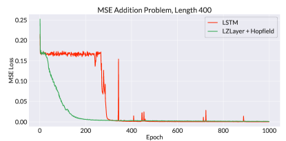
Figure 2: Addition problem results — LZ Layer with Hopfield Associative Memory.

Although the initial results from the LZHOP Layer were very promising, this model was not scalable to longer sequence lengths because the Hopfield Network associative memory had quadratic run-time behavior. We next turned our attention to associative models requiring less computational overhead, with the hope that they would replicate the improvements achieved in the LZHOP Layer. We began with the LZ Layer with a VTB Associative Memory and LSTM RNN cell (LZVTB). In each experiment, we use a batch size of 50, with a hidden size of 256, as the VTB memory requires that the hidden size be a perfect square. Again, we use an RMSProp optimizer with a learning rate of $10^{-3}$ and a decay rate of 0.9 and compare our results to a traditional LSTM with the same parameters. In Figure 3, we see that the LZVTB Layer also reaches error rates comparable to those of an LSTM, and is still able to train in fewer epochs. However, there are occasional dramatic spikes in the loss, indicating undesirable unstable behavior in the model. We believe this behavior occurred because not every vector inserted into the VTB Associative Memory was orthogonal.

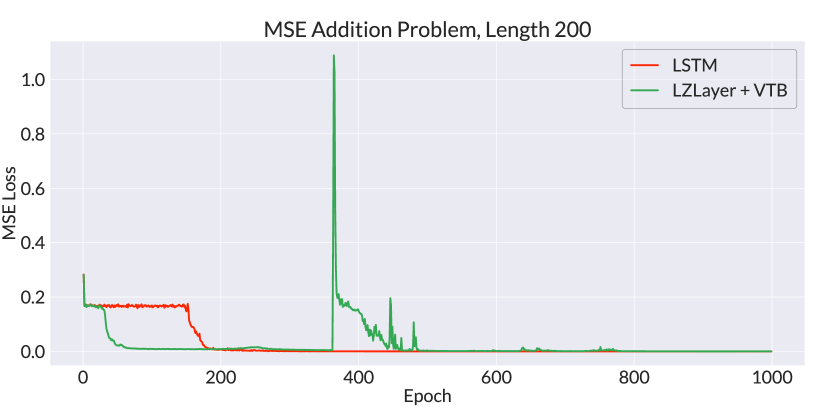
Figure 3: Addition problem results — LZ Layer with VTB Associative Memory

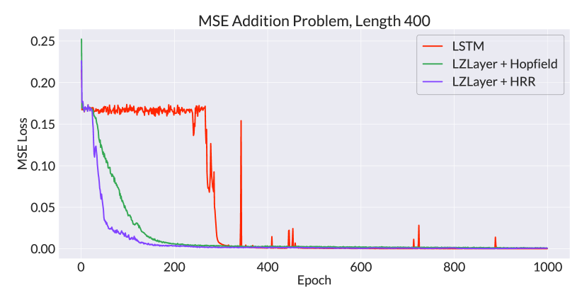
Figure 4: Addition problem results — LZ Layer with HRR Associative Memory

To address some of the stability issues with the VTB Associative Memory, we turned to a new, HRR-based associative memory. We used the same parameters as in the LZHOP experiments, to enable easy comparison of the results, and found that an LZ Layer with an HRR Associative Memory and LSTM RNN cell (LZHRR) was able to replicate the stability of the LZHOP model while being less computationally expensive and requiring less memory. In addition to approaching comparable error rates, the LZHRR model also required fewer epochs to train than the LZHOP model (see Figure 4). This evidence persuaded us that the LZHRR model would be a viable approach to many sequence processing problems.

UCR Time Series Archive

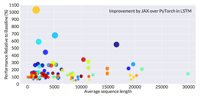
(a) LSTM

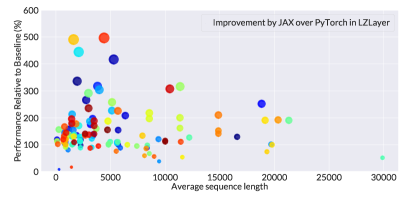
(b) LZLayer

Figure 9: Accuracy improvement from JAX over PyTorch implementation in both LSTM (a) and LZLayer (b). Points above 100% indicate datasets on which the implementation in JAX outperformed the implementation in PyTorch. The accuracy of the LSTM is improved in $69.53\%$ of the datasets and the accuracy of the LZ Layer is improved in $79.68\%$ of the datasets. The size of the circle is proportional to the amount of improvement.

The UCR Time Series Archive [17] is a collection of 128 datasets for time series classification problems created to ameliorate the phenomenon of cherry-picking datasets that yield good results in ML research. We trained an LZHRR model, along with an LSTM baseline model, on every single dataset in the UCR Archive, and the full results are shown in Table 3 in Appendix A. For both the LZ Layer and the LSTM, we chose a hidden size of 256. The models were trained using the Adam optimizer with a learning rate of $10^{-3}$ for 500 epochs. For the LZ Layer, we additionally tested the performance with various bias $b$ initializations over the Bilinear layer, where $b\in\{0,1,-1\}$. Figure LABEL:fig:improve_bias shows the differences in accuracy between the LZ Layer and the LSTM on the UCR datasets. Overall, the LZ Layer outperforms a traditional LSTM in $46.88\%$ of the datasets, but there are instances in which it significantly underperforms the LSTM. Moreover, to run the UCR trials, we implemented our LZ Layer and LSTM in both PyTorch and JAX, the deep learning library from Google. Implementation in JAX dramatically improved the performance of both models in terms of computational time and accuracy. The accuracy improvement is shown in Figure 9 in Appendix A — LSTM accuracy is improved on 69.53% of datasets, and LZ Layer accuracy is improved on 79.68% of datasets.

PS-MNIST

Permuted Sequential MNIST (PS-MNIST) [18] is another benchmark for comparing recurrent networks, in which the $784$ pixels of the MNIST images are presented sequentially to an RNN following the application of a fixed permutation. We tested the LZHRR layer on the PS-MNIST dataset and compared its performance to that of an LSTM and the Shuffle RNN (SRNN) from [16]. All the recurrent networks were trained with a hidden size of 256 and a batch size of 64. The models were optimized using the Adam optimizer with a learning rate of $10^{-4}$ for 300 epochs. Figure 5 shows the accuracy curve on the test set of all three models. The performance of LZLayer on PS-MNIST is better than SRNN and close to LSTM.

5 Conclusions

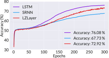
Figure 5: Accuracy curve of the LZLayer, LSTM, and SRNN on the test set of PS-MNIST.

This paper proposes a novel RNN for processing long sequences, where we pair a traditional LSTM cell with an associative memory to mimic the process of LZ compression. We experimented with Hopfield Network, VTB, and HRR associative memories and ultimately settled on HRR as providing the best combination of stability, speed, and memory usage. After running our LZHRR layer on all 128 datasets of the UCR Time Series Archive, we found that the LZ network generally underperforms a traditional LSTM, regardless of sequence length. We hypothesize that this is because the HRR process is too noisy to replicate the function of the external memory in LZ compression faithfully. However, more robust associative memories come with an additional set of runtime and memory challenges, as hinted at by our experiments with Hopfield associative memories.

To improve the speed of the LZ Layer, we transitioned its code from PyTorch to JAX. To facilitate a fair comparison, we did the same for the LSTM baselines, which had been developed in PyTorch by other researchers in this area. We were surprised to find that our re-implementation improved both the runtime and the accuracy of the original baseline models. While our baselines where selected from respectable, published work [16], our results highlight that using baselines naively from prior works can lead our evaluations and conclusions astray. We hypothesize that this may be in part due to the niceness of the research area, as fewer people have spent time tuning these baselines to ensure robust performance. This mimics problems recently seen in other areas of ML reproducibility, where we have observed that improving the baselines mitigates any benefits of the new technique, resulting in “false discoveries” [19, 20, 21, 22] and increasing the effort required to replicate results [23, 24].

Appendix A Supplemental Results

A.1 Addition problem

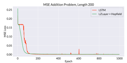
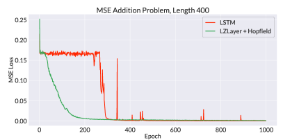
Figure 6: Addition problem results — LZ Layer with Hopfield Associative Memory.

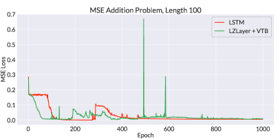
Figure 7: Addition problem results — LZ Layer with VTB Associative Memory.

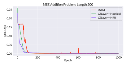
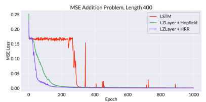
Figure 8: Addition problem results — LZ Layer with HRR Associative Memory.

A.2 UCR Time Series Archive

Table 3: UCR Dataset

Dataset	LSTM	LZLayer $b=0$	LZLayer $b=1$	LZLayer $b=-1$	Dataset	LSTM	LZLayer $b=0$	LZLayer $b=1$	LZLayer $b=-1$
ACSF1	55.0	44.0	43.0	51.0	Adiac	72.38	64.45	51.92	70.08
AllGestureWiimoteX	41.0	41.43	40.14	40.71	AllGestureWiimoteY	53.29	53.29	50.14	52.57
AllGestureWiimoteZ	44.57	41.71	38.57	43.57	ArrowHead	78.86	80.57	81.14	83.43
Beef	90.0	83.33	83.33	83.33	BeetleFly	85.0	85.0	90.0	85.0
BirdChicken	70.0	70.0	70.0	70.0	BME	79.33	81.33	81.33	80.0
Car	85.0	83.33	78.33	81.67	CBF	87.44	88.44	87.89	87.78
Chinatown	97.38	97.38	97.67	97.08	ChlorineConcentration	83.33	74.74	66.72	80.26
CinCECGTorso	81.96	83.12	82.25	83.48	Coffee	100.0	100.0	100.0	100.0
Computers	58.4	57.2	56.8	56.8	CricketX	56.15	53.85	47.44	55.38
CricketY	60.26	57.18	56.15	59.23	CricketZ	58.21	55.13	50.77	56.92
Crop	72.1	4.17	69.71	73.16	DiatomSizeReduction	95.75	95.42	95.75	96.41
DistalPhalanxOutlineAgeGroup	73.38	70.5	71.94	70.5	DistalPhalanxOutlineCorrect	71.38	73.55	73.91	72.83
DistalPhalanxTW	64.75	65.47	66.19	69.06	DodgerLoopDay	56.25	62.5	61.25	55.0
DodgerLoopGame	83.33	84.06	84.78	84.78	DodgerLoopWeekend	98.55	98.55	98.55	97.1
Earthquakes	67.63	66.19	66.91	64.75	ECG200	90.0	90.0	89.0	90.0
ECG5000	93.2	93.16	92.82	93.13	ECGFiveDays	96.05	96.05	96.52	96.17
ElectricDevices	49.7	54.69	53.56	53.4	EOGHorizontalSignal	43.37	40.06	37.29	43.65
EOGVerticalSignal	27.07	8.29	25.41	8.29	EthanolLevel	68.6	25.2	25.2	25.2
FaceAll	81.83	79.23	78.82	80.83	FaceFour	84.09	86.36	85.23	85.23
FacesUCR	79.85	79.37	79.07	80.2	FiftyWords	70.99	66.15	62.42	69.89
Fish	85.14	86.86	87.43	86.29	FordA	78.94	74.17	74.32	72.88
FordB	70.62	68.4	68.77	64.2	FreezerRegularTrain	93.19	93.16	92.98	93.16
FreezerSmallTrain	69.58	68.74	68.6	68.67	Fungi	85.48	86.02	85.48	85.48
GestureMidAirD1	53.08	54.62	53.08	55.38	GestureMidAirD2	52.31	53.85	55.38	54.62
GestureMidAirD3	24.62	19.23	15.38	19.23	GesturePebbleZ1	85.47	84.3	86.05	84.88
GesturePebbleZ2	75.95	72.78	72.78	72.78	GunPoint	94.67	94.0	94.0	94.0
GunPointAgeSpan	94.3	89.24	87.97	90.82	GunPointMaleVersusFemale	99.68	99.37	99.05	99.05
GunPointOldVersusYoung	100.0	100.0	100.0	100.0	Ham	66.67	67.62	66.67	67.62
HandOutlines	91.89	35.95	35.95	35.95	Haptics	43.51	42.86	41.56	44.81
Herring	64.06	65.62	59.38	62.5	HouseTwenty	73.11	72.27	72.27	73.95
InlineSkate	34.55	33.64	29.82	34.73	InsectEPGRegularTrain	100.0	100.0	100.0	100.0
InsectEPGSmallTrain	100.0	100.0	99.6	100.0	InsectWingbeatSound	63.08	63.43	62.93	62.93
ItalyPowerDemand	95.53	96.4	97.08	95.72	LargeKitchenAppliances	43.2	43.2	42.93	42.4
Lightning2	67.21	68.85	70.49	67.21	Lightning7	64.38	65.75	64.38	63.01
Mallat	92.71	92.2	92.71	92.03	Meat	91.67	81.67	65.0	90.0
MedicalImages	70.66	71.32	68.55	70.39	MelbournePedestrian	92.78	90.45	88.56	91.84
MiddlePhalanxOutlineAgeGroup	52.6	55.84	61.04	58.44	MiddlePhalanxOutlineCorrect	76.29	81.44	78.69	80.41
MiddlePhalanxTW	53.25	56.49	54.55	50.65	MixedShapesRegularTrain	90.68	88.21	88.74	88.91
MixedShapesSmallTrain	84.0	84.16	83.22	84.54	MoteStrain	85.46	86.42	86.9	87.06
NonInvasiveFetalECGThorax1	92.77	90.94	87.18	90.64	NonInvasiveFetalECGThorax2	92.72	90.64	87.33	92.52
OliveOil	76.67	40.0	40.0	56.67	OSULeaf	53.72	51.24	53.72	52.07
PhalangesOutlinesCorrect	79.14	75.99	75.29	78.32	Phoneme	10.07	9.97	8.97	10.02
PickupGestureWiimoteZ	68.0	68.0	66.0	62.0	PigAirwayPressure	10.1	10.1	10.1	8.17
PigArtPressure	21.63	20.19	22.12	21.15	PigCVP	11.06	11.06	11.54	12.02
PLAID	44.13	43.58	41.53	44.69	Plane	98.1	98.1	96.19	98.1
PowerCons	100.0	100.0	100.0	100.0	ProximalPhalanxOutlineAgeGroup	80.49	85.37	83.9	82.93
ProximalPhalanxOutlineCorrect	85.22	81.44	81.79	82.47	ProximalPhalanxTW	80.0	81.95	79.02	80.0
RefrigerationDevices	38.93	35.2	36.27	38.67	Rock	60.0	50.0	44.0	54.0
ScreenType	38.4	39.73	42.93	38.13	SemgHandGenderCh2	90.17	90.17	90.17	88.67
SemgHandMovementCh2	67.56	58.67	62.22	67.33	SemgHandSubjectCh2	89.33	86.44	87.11	88.44
ShakeGestureWiimoteZ	56.0	64.0	54.0	60.0	ShapeletSim	49.44	47.78	50.0	56.11
ShapesAll	75.0	73.0	68.5	72.83	SmallKitchenAppliances	37.07	35.73	38.13	37.33
SmoothSubspace	90.0	89.33	88.0	89.33	SonyAIBORobotSurface1	72.55	71.71	71.05	71.55
SonyAIBORobotSurface2	82.9	82.69	82.79	82.9	StarLightCurves	91.68	93.19	90.0	92.98
Strawberry	96.22	96.49	35.68	95.95	SwedishLeaf	84.96	7.36	81.76	82.72
Symbols	87.04	86.33	86.33	86.33	SyntheticControl	92.0	90.0	89.33	91.0
ToeSegmentation1	58.77	59.65	59.65	61.4	ToeSegmentation2	76.92	77.69	76.15	76.92
Trace	77.0	77.0	64.0	77.0	TwoLeadECG	90.43	84.64	82.18	85.34
TwoPatterns	92.48	91.73	90.42	92.38	UMD	92.36	94.44	95.14	94.44
UWaveGestureLibraryAll	95.42	94.78	94.03	95.06	UWaveGestureLibraryX	76.35	74.4	72.84	74.96
UWaveGestureLibraryY	69.1	67.11	65.69	68.43	UWaveGestureLibraryZ	69.71	66.78	66.08	67.53
Wafer	99.61	99.56	99.56	99.56	Wine	75.93	70.37	48.15	72.22
WordSynonyms	58.46	59.09	55.96	59.09	Worms	51.95	49.35	42.86	51.95
WormsTwoClass	59.74	63.64	61.04	66.23	Yoga	84.87	83.7	83.87	85.1

A.3 JAX v PyTorch

A.4 Memory copy problem

The LZHRR layer, implemented in PyTorch, was also tested on the memory copy problem. Though the results were not particularly revealing, we include them here in the appendix for completeness.

The copy problem tests an RNN’s ability to memorize the first $N$ items in a long sequence. As input, the RNN receives a sequence of $N$ significant items, drawn from a fixed set $M$ of symbols, followed by $T-1$ “blank” inputs, a special delimiter symbol, and $N$ more blank items. The desired output is $N+T$ blank symbols, followed by the $N$ original significant items (see Table 4). We compare to a baseline model which outputs a constant sequence after it sees the delimiter symbol; this base solution has a cross-entropy of $\frac{N\ln M}{T+2N}$.

In conjunction with [16], we chose parameters of $N=10$, $M=8$, a batch size of 20, and a hidden size of 128. We tested $T=100,200,300,500,1000,$ and $2000$, training each model for 1000 epochs. Again, we use the RMSProp optimizer with a learning rate of $10^{-3}$ and a decay rate of 0.9, and a model with only one LZ Layer. We also include results from a traditional LSTM, trained with the same parameters, for an additional point of comparison.

For every choice of $T$, the LSTM outperformed the LZ Layer. However, as the sequence length increased, the gap between the performance of the LZ Layer and that of the LSTM shrunk. Interestingly, this was not due to LSTM performance deteriorating as the sequences lengthened but rather because the LZ Layer improved significantly.

Table 4: Sample input and output for the copy problem with $N=5$, $M=3$, $T=10$. $\star$ denotes a special delimiter symbol; in practice, it can be a digit not used in the memorization sequence.

1

2

3

2

1

0

0

0

0

0

0

0

0

0

$\star$

0

0

0

0

0

0

0

0

0

0

0

0

0

0

0

0

0

0

0

0

1

2

3

2

1

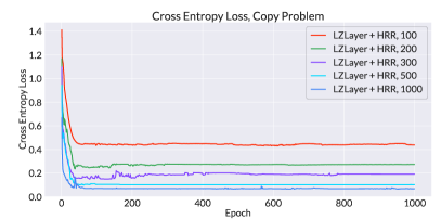
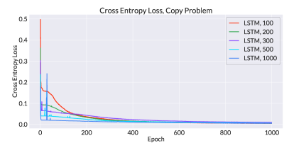
Figure 10: Cross entropy losses on the memory copy problem with varying sequence lengths for an LZ Layer with HRR Associative Memory (left) and an LSTM (right).

References

- Hochreiter and Schmidhuber [1997] S. Hochreiter and J. Schmidhuber, “Long Short-Term Memory,” Neural Computation, vol. 9, no. 8, pp. 1735–1780, 11 1997. [Online]. Available: http://www.mitpressjournals.org/doi/abs/10.1162/neco.1997.9.8.1735
- Yu et al. [2019] Y. Yu, X. Si, C. Hu, and J. Zhang, “A review of recurrent neural networks: Lstm cells and network architectures,” Neural Computation, vol. 31, no. 7, pp. 1235–1270, 2019.
- Trinh et al. [2018] T. Trinh, A. Dai, T. Luong, and Q. Le, “Learning longer-term dependencies in rnns with auxiliary losses,” in International Conference on Machine Learning. PMLR, 2018, pp. 4965–4974.
- Lipton et al. [2015] Z. C. Lipton, J. Berkowitz, and C. Elkan, “A critical review of recurrent neural networks for sequence learning,” arXiv preprint arXiv:1506.00019, 2015.
- Raff and Nicholas [2017] E. Raff and C. Nicholas, “An Alternative to NCD for Large Sequences, Lempel-Ziv Jaccard Distance,” in KDD, 2017, pp. 1007–1015. [Online]. Available: http://dl.acm.org/citation.cfm?doid=3097983.3098111
- Raff and Nicholas [2018] E. Raff and C. K. Nicholas, “Lempel-ziv jaccard distance, an effective alternative to ssdeep and sdhash,” Digital Investigation, Feb 2018.
- [7] J. Aurelio, E. Raff, and C. Nicholas, “Pylzjd: An easy to use tool for machine learning,” in Proceedings of the 18th Python in Science Conference. [Online]. Available: http://conference.scipy.org/proceedings/scipy2019/pylzjd.html
- [8] “Malware classification and class imbalance via stochastic hashed lzjd,” in Proceedings of the 10th ACM Workshop on Artificial Intelligence and Security.
- Hopfield [1982] J. J. Hopfield, “Neural networks and physical systems with emergent collective computational abilities,” Proceedings of the National Academy of Sciences, vol. 79, no. 8, pp. 2554–2558, 1982.
- Ramsauer et al. [2020] H. Ramsauer, B. Schäfl, J. Lehner, P. Seidl, M. Widrich, T. Adler, L. Gruber, M. Holzleitner, M. Pavlović, G. K. Sandve et al., “Hopfield networks is all you need,” arXiv preprint arXiv:2008.02217, 2020.
- Schlegel et al. [2020] K. Schlegel, P. Neubert, and P. Protzel, “A comparison of vector symbolic architectures,” arXiv preprint arXiv:2001.11797, 2020.
- Gosmann and Eliasmith [2019] J. Gosmann and C. Eliasmith, “Vector-derived transformation binding: an improved binding operation for deep symbol-like processing in neural networks,” Neural Computation, vol. 31, no. 5, pp. 849–869, 2019.
- Plate [1995] T. A. Plate, “Holographic reduced representations,” IEEE Transactions on Neural Networks, vol. 6, no. 3, pp. 623–641, 1995.
- Ganesan et al. [2021] A. Ganesan, H. Gao, S. Gandhi, E. Raff, T. Oates, J. Holt, and M. McLean, “Learning with holographic reduced representations,” in Advances in Neural Information Processing Systems, A. Beygelzimer, Y. Dauphin, P. Liang, and J. W. Vaughan, Eds., 2021. [Online]. Available: https://openreview.net/forum?id=RX6PrcpXP-
- Alam et al. [2022] M. M. Alam, E. Raff, T. Oates, and J. Holt, “Deploying Convolutional Networks on Untrusted Platforms Using 2D Holographic Reduced Representations,” in International Conference on Machine Learning, 2022. [Online]. Available: http://arxiv.org/abs/2206.05893
- Rotman and Wolf [2020] M. Rotman and L. Wolf, “Shuffling recurrent neural networks,” arXiv preprint arXiv:2007.07324, 2020.
- Dau et al. [2018] H. A. Dau, E. Keogh, K. Kamgar, C.-C. M. Yeh, Y. Zhu, S. Gharghabi, C. A. Ratanamahatana, Yanping, B. Hu, N. Begum, A. Bagnall, A. Mueen, G. Batista, and Hexagon-ML, “The ucr time series classification archive,” October 2018, https://www.cs.ucr.edu/~eamonn/time_series_data_2018/.
- Le et al. [2015] Q. V. Le, N. Jaitly, and G. E. Hinton, “A simple way to initialize recurrent networks of rectified linear units,” arXiv preprint arXiv:1504.00941, 2015.
- Musgrave et al. [2020] K. Musgrave, S. Belongie, and S.-N. Lim, “A Metric Learning Reality Check,” in ECCV, 2020. [Online]. Available: http://arxiv.org/abs/2003.08505
- Blalock et al. [2020] D. Blalock, J. J. Gonzalez Ortiz, J. Frankle, and J. Guttag, “What is the State of Neural Network Pruning?” in Proceedings of Machine Learning and Systems 2020, 2020, pp. 129–146.
- Dacrema et al. [2019] M. F. Dacrema, P. Cremonesi, and D. Jannach, “Are we really making much progress? A Worrying Analysis of Recent Neural Recommendation Approaches,” in Proceedings of the 13th ACM Conference on Recommender Systems - RecSys ’19. New York, New York, USA: ACM Press, 2019, pp. 101–109. [Online]. Available: http://dl.acm.org/citation.cfm?doid=3298689.3347058
- Bouthillier et al. [2021] X. Bouthillier, P. Delaunay, M. Bronzi, A. Trofimov, B. Nichyporuk, J. Szeto, N. Sepah, E. Raff, K. Madan, V. Voleti, S. E. Kahou, V. Michalski, D. Serdyuk, T. Arbel, C. Pal, G. Varoquaux, and P. Vincent, “Accounting for Variance in Machine Learning Benchmarks,” in Machine Learning and Systems (MLSys), 2021. [Online]. Available: http://arxiv.org/abs/2103.03098
- Raff [2021] E. Raff, “Research Reproducibility as a Survival Analysis,” in The Thirty-Fifth AAAI Conference on Artificial Intelligence, 2021. [Online]. Available: http://arxiv.org/abs/2012.09932
- Raff and Farris [2022] E. Raff and A. L. Farris, “A Siren Song of Open Source Reproducibility,” in ML Evaluation Standards Workshop at ICLR 2022, 2022. [Online]. Available: https://arxiv.org/abs/2204.04372