Deterministic generation of qudit photonic graph states from quantum emitters

Abstract

We propose and analyze deterministic protocols to generate qudit photonic graph states from quantum emitters. We exemplify our approach by constructing protocols to generate absolutely maximally entangled states and logical states of quantum error correcting codes. Some of these protocols make use of time-delayed feedback, while others do not. These results significantly broaden the range of multi-photon entangled states that can be produced deterministically from quantum emitters.

I Introduction

Entanglement is a uniquely quantum property that plays an important role in almost all aspects of quantum information science, including quantum computing Horodecki et al. [2009], quantum error correction Scott [2004], Calderbank et al. [1998], quantum sensing Degen et al. [2017], and quantum networks Cirac et al. [1997], Kimble [2008], Hillery et al. [1999]. Many of these applications require generating large multi-photon entangled resource states upfront, especially in the context of measurement- or fusion-based quantum computing Raussendorf and Briegel [2001a], Bartolucci et al. [2021], Omkar et al. [2022] and quantum communication Gisin and Thew [2007], Azuma et al. [2015], Zwerger et al. [2016], Muralidharan et al. [2016].

However, creating entangled states of many photons is challenging because photons do not interact directly. Standard ways of circumventing this issue make use of either nonlinear media Guerreiro et al. [2014] or quantum interference and measurement Knill and Milburn [2001], Kok et al. [2007]; the former approach is made challenging by low coupling efficiencies, while the latter is intrinsically probabilistic. Approaches that rely on interfering photons are usually based on linear optics and post-selection Knill and Milburn [2001], Kok et al. [2007], and consequently the success probability decreases exponentially with the number of photons Knill and Milburn [2001], Bodiya and Duan [2006]. Despite a number of conceptual and technological advances, the probabilistic nature of this approach continues to severely limit the size of multi-photon entangled states constructed in this way Gao et al. [2010], Li et al. [2020].

An alternative approach is to use coupled, controllable quantum emitters with suitable level structures to deterministically generate multi-photon entanglement Schön et al. [2005], Lindner and Rudolph [2009a], Economou et al. [2010a]. There now exist several explicit protocols for creating entangled states of many photonic qubits, either by using entangling gates between emitters and transferring entanglement to the photons in the photon emission stage Economou et al. [2010a], Buterakos et al. [2017], Russo et al. [2019a], Gimeno-Segovia et al. [2019a], Hilaire et al. [2021], Liu et al. [2022], Li et al. [2022], or by (re)interfering photons with emitters to create entanglement beyond that potentially generated through the emission process Wiseman and Milburn [2009], Pichler et al. [2017], Zhan and Sun [2020], Shi and Waks [2021a]. Proof-of-principle experimental demonstrations of such deterministic protocols have been performed in both the optical and microwave domains Schwartz et al. [2016], Besse et al. [2020], Thomas et al. [2022], Coste et al. [2022].

To date, the vast majority of theoretical and experimental efforts towards the deterministic generation of multi-photon entangled states have focused on photonic qubits. These are based on using either polarization, spatial path, or time bin as the logical encoding. However, photons can naturally encode not only qubits but also multi-dimensional qudit states, for example by using more than two spatial paths or time bins. This can allow for novel approaches to quantum computing, communication, sensing, and error correction in which quantum information is stored in a more compact way Kues et al. [2017], Erhard et al. [2020], Wang et al. [2020]. Such states can in particular provide benefits in quantum networks and repeaters Muralidharan et al. [2018], Zheng et al. [2022]. Although there have been recent experimental demonstrations of entangled qudit state creation, these have been limited thus far to two photons Kues et al. [2017], Reimer et al. [2019]. An outstanding question is whether multi-photon entangled qudit states can be generated deterministically from a small number of quantum emitters.

In this paper, we propose and evaluate deterministic methods to generate multi-photon qudit graph states from multi-level quantum emitters. We present several different explicit protocols that can produce various states either using a single emitter together with time-delayed feedback, or using multiple coupled quantum emitters. While our approach is quite general, here we focus on constructing highly entangled multipartite states called absolutely maximally entangled (AME) states. These states are defined by the property that they maximize the entanglement entropy for any bipartition Helwig et al. [2012], Helwig and Cui [2013], and they have applications in quantum error correcting codes (QECCs) and secret sharing Scott [2004], Helwig et al. [2012], Helwig and Cui [2013], Raissi et al. [2018], Goyeneche et al. [2018], Raissi et al. [2020], Raissi [2020], Raissi et al. [2021]. In addition, we present protocols for constructing logical states of QECCs whose code spaces are spanned by AME states of qutrits.

The paper is organized as follows. We begin with a brief review of qudit graph states and describe the basic operations needed to create them from quantum emitters (Sec. II). In Sec. III, we describe how to produce photonic qudits from quantum emitters and illustrate our basic approach to multi-qudit-state generation by presenting a protocol to create one-dimensional qudit graph states. In Sec. IV, we present protocols for generating various AME states. Finally, in Sec. V, we show how to generate an explicit example of a QECC whose codewords are all AME states of qutrits. We conclude in Sec. VII.

II Background: qudits and graph states

In this work, we focus on the generation of an important class of entangled states called graph states Hein et al. [2006]. Graph states are pure quantum states that are defined based on a graph $G=(V,\Gamma)$, which is composed of a set $V$ of $n$ vertices (each qudit is represented by a vertex), and a set of edges specified by the adjacency matrix $\Gamma$. $\Gamma$ is an $n\times n$ symmetric matrix such that $\Gamma_{i,j}=0$ if vertices $i$ and $j$ are not connected and $\Gamma_{i,j}>0$ otherwise Van den Nest et al. [2004], Hein et al. [2004, 2006], Bahramgiri and Beigi [2006]. These states have many applications in measurement-based quantum computing Raussendorf and Briegel [2001b], Bartolucci et al. [2021], quantum networks Azuma et al. [2015], Zwerger et al. [2016], Muralidharan et al. [2016], and QECCs Gottesman [1997, 2009].

There are differences between qubit and qudit graph states. For the qubit case, the graph state is defined by initializing all qubits in the $+1$ eigenstate of the $X$ Pauli matrix, i.e., the state $|+\rangle=|0\rangle+|1\rangle$ (here and in the following we will not always explicitly normalize states for the sake of a more compact notation), and then applying controlled-$Z$ ($CZ$) gates on all pairs of qubits connected by an edge. In the case of qubits, the adjacency matrix $\Gamma$ contains two different elements: $\Gamma_{i,j}=0$ whenever two vertices $i$ and $j$ are not connected, and $\Gamma_{i,j}=1$ otherwise. Most of the existing protocols for creating multi-photon entangled states have focused on the generation of multi-qubit graph states Lindner and Rudolph [2009a], Economou et al. [2010a], Buterakos et al. [2017], Russo et al. [2019a], Gimeno-Segovia et al. [2019a], Hilaire et al. [2021], Liu et al. [2022], Li et al. [2022], Pichler et al. [2017], Zhan and Sun [2020], Shi and Waks [2021a].

To define qudit graph states, we first introduce generalized Pauli operators acting on qudits with $q$ levels Bahramgiri and Beigi [2006]. The Pauli operators $X$ and $Z$ act on the eigenstates of $Z$ as follows:

$$X|i\rangle =|i+1\mod q\rangle,$$ (1)

$$Z|i\rangle =\omega^{i}\,|i\rangle\,.$$ (2)

These operators are unitary and traceless, and they satisfy the condition $ZX=\omega XZ$, where $\omega=\operatorname{\mathrm{e}}^{\operatorname{\mathrm{i}}2\pi/q}$ is a $q$-th root of unity. Each of the Pauli matrices has $q$ eigenvalues and eigenvectors. The powers of $X$ and $Z$ applied to basis states give

$$X^{\alpha}|i\rangle =|i+\alpha\mod q\rangle,$$ (3)

$$Z^{\beta}|i\rangle =\omega^{i\beta}\,|i\rangle\,,$$ (4)

and $X^{q}=Z^{q}=\mathbbm{1}$. Similar to the case of qubits, we can define controlled-$Z^{\beta}$ ($CZ^{\beta}$) gates as

$$CZ^{\beta}|i,j\rangle=\omega^{\beta\,ij}|i,j\rangle,\qquad\forall\beta\in\{1,\dots,q-1\}\ .$$ (5)

The special case of $q=2$ in the above corresponds to qubits.

One other operator that is essential to studying qudit graph states is the Hadamard gate. The Hadamard gate $H$ is a matrix that maps the $Z$-eigenbasis into the $X$-eigenbasis. For qubits, we have $H|0\rangle=|+\rangle$, and $H|1\rangle=|-\rangle$, where $|-\rangle$ is the $-1$ eigenvector of the $X$ Pauli operator. There is also a useful identity involving the Hadamard and the Pauli matrices $X$ and $Z$: $HXH=Z$.

Similarly to the qubit case, we can define the qudit Hadamard operator $H$ such that $H|i\rangle=|X_{i}\rangle$, where $|X_{i}\rangle$ is an eigenstate of $X$. In general, we can write

$$H|i\rangle=\sum_{j=0}^{q-1}\omega^{ij}|j\rangle=|X_{i}\rangle\qquad\forall i\in\{0,1,...,q-1\}\ .$$ (6)

The relationship between the Hadamard and the Pauli operators $X^{\alpha}$ and $Z^{\alpha}$ in the case of qudits takes the form

$$HX^{\alpha}H^{\dagger}=Z^{\alpha},$$ (7)

where $H^{\dagger}$ is the inverse of $H$:

$$H^{\dagger}|i\rangle=\sum_{j=0}^{q-1}\omega^{(q-1)ij}|j\rangle=|X_{q-i\!\!\!\!\mod q}\rangle,\quad i=0,...,q-1$$ (8)

Also note that $H^{\dagger}$ acts on the $X$-eigenbasis as $H^{\dagger}|X_{i}\rangle=|i\rangle$.

To understand how we can use these ingredients to define qudit graph states, we present an explicit example involving qutrits. A qutrit is realized by a 3-level quantum system ($q=3$), where we denote the $Z$-eigenstates by $|0\rangle$, $|1\rangle$, and $|2\rangle$. The $X$-eigenstates then are

$$|X_{0}\rangle =|0\rangle+|1\rangle+|2\rangle,$$ (9)

$$|X_{1}\rangle =|0\rangle+\omega|1\rangle+\omega^{2}|2\rangle,$$ (10)

$$|X_{2}\rangle =|0\rangle+\omega^{2}|1\rangle+\omega|2\rangle\ ,$$ (11)

where $\omega=e^{\operatorname{\mathrm{i}}2\pi/3}$. The $X$ operator couples levels as follows: $X|i\rangle=|i+1\mod 3\rangle$ and $X^{2}|i\rangle=|i+2\mod 3\rangle$. The $Z$ and $Z^{2}$ operators add different phase factors to each basis state, i.e., $Z|i\rangle=\omega^{i}|i\rangle$ and $Z^{2}|i\rangle=\omega^{2i}|i\rangle$, while $X^{3}=\mathbbm{1}$ and $Z^{3}=\mathbbm{1}$.

In order to obtain qutrit graph states, we first initialize all qutrits in state $|X_{0}\rangle$. For each edge, we can consider two possible gates on the corresponding qutrits: $CZ$ and $CZ^{2}$, which are defined such that

$$CZ|i,j\rangle =\omega^{ij}|i,j\rangle,$$ (12)

$$CZ^{2}|i,j\rangle =\omega^{2\,ij}|i,j\rangle,$$ (13)

where $i,j\in\{0,1,2\}$. Therefore, the adjacency matrix $\Gamma$ contains three different elements, $\Gamma_{i,j}=0$ when the two vertices $i$ and $j$ are not connected, $\Gamma_{i,j}=1$ when they are connected via $CZ$, and $\Gamma_{i,j}=2$ when they are connected via $CZ^{2}$.

III Emitting photonic qudits and linear graph states

In addition to qudit operations, another key ingredient we need to generate qudit photonic graph states is a “pumping” operation that produces photonic qudits from quantum emitters. In this section, we explain how such operations can be realized in systems containing multi-level emitters with the appropriate level structure and selection rules. Later on in Sec. VI, we give explicit examples of such systems, which include color centers in solids and trapped ions. In the present section, we also illustrate how photon pumping, together with qudit operations on emitters and photons, can be used to deterministically create entanglement between photonic qudits.

As a warm-up example illustrating how this works, in this section we present protocols for generating one-dimensional (1D) qudit graph states using a single quantum emitter with an appropriate level structure. This example is closely related to Ref. Lindner and Rudolph [2009b], which showed how to produce a qubit 1D graph state from an emitter comprised of a single electron spin in an optically active quantum dot. That work introduced a protocol in which each photon emission is preceded by a Hadamard gate. Repeating the basic sequence of Hadamard gate followed by optical pumping/photon emission $n$ times results in a $n$-qubit linear graph state. Because each photon emission can be viewed as a $CNOT$ gate acting on the emitter and emitted photon, this operation together with the Hadamard gates effectively generates the requisite $CZ$ gate between neighboring photonic qubits.

Although the original proposal of Ref. Lindner and Rudolph [2009b] focused on using photon polarization as the qubit degree of freedom, it is important to note that one can also generate a linear graph state based on time-bin qubits by using circularly (rather than linearly) polarized light to pump the emitter and by including a few additional operations during each cycle of the protocol Lee et al. [2019]. In this protocol, only one of the emitter ground states, say $|0\rangle_{\text{e}}$, can be optically excited by the pump, so that an initial superposition state $|0\rangle_{\text{e}}+|1\rangle_{\text{e}}$ becomes $|0\rangle_{\text{e}}|0\rangle_{\text{p}}+|1\rangle_{\text{e}}|\text{vac}\rangle$ after the first photon emission, where $|0\rangle_{\text{p}}$ corresponds to a photon in the first time bin, while $|\text{vac}\rangle$ represents the vacuum. If we then apply an $X$ gate on the emitter and perform a second optical pumping operation, we obtain $|1\rangle_{\text{e}}|0\rangle_{\text{p}}+|0\rangle_{\text{e}}|1\rangle_{\text{p}}$, where $|1\rangle_{\text{p}}$ corresponds to a photon in the second time bin.

The above protocol for time-bin qubits naturally extends to time-bin qudits with local dimension $q$, provided we have at our disposal a quantum emitter with $q$ energy levels comprising the ground state manifold, one of which is optically coupled to an excited state. As in the qubit case, upon emission these photonic time-bin qudits will be entangled with the emitter. In general, the cyclic transitions commonly used for optical readout of various qudit systems can be used to optically pump photonic time-bin qudits with $q$ levels through a straightforward generalization of the pumping procedure described above for qubits. For example, consider a three-level quantum emitter with states $|0\rangle_{\text{e}}$, $|1\rangle_{\text{e}}$, $|2\rangle_{\text{e}}$. By starting from an initial equal superposition state $|0\rangle_{\text{e}}+|1\rangle_{\text{e}}+|2\rangle_{\text{e}}$ and interspersing three such pumping/emission events by gate operations that rotate the three different emitter ground states into one another, one can obtain the state $|0\rangle_{\text{e}}|0\rangle_{\text{p}}+|1\rangle_{\text{e}}|1\rangle_{\text{p}}+|2\rangle_{\text{e}}|2\rangle_{\text{p}}$, where $|0\rangle_{\text{p}}$, $|1\rangle_{\text{p}}$, $|2\rangle_{\text{p}}$ are three different photonic time-bin states. We denote this net photon-pumping operation by

$${\cal P}_{\mathrm{pump}}(|0\rangle_{\text{e}}+|1\rangle_{\text{e}}+|2\rangle_{\text{e}})=|0\rangle_{\text{e}}|0\rangle_{\text{p}}+|1\rangle_{\text{e}}|1\rangle_{\text{p}}+|2\rangle_{\text{e}}|2\rangle_{\text{p}}.$$ (14)

This operation (and its natural generalization to $q$ time bins) is a central ingredient in the protocols that follow.

Focusing on the qutrit case for concreteness, we now show how to produce linear graph states using Eq. (14). In addition to this photon-pumping operation, we also need to use the qutrit Hadamard operator $H$ in order to obtain the desired entanglement structure in the final multi-photon state. Unlike in the qubit case, in the case of qutrits there are multiple types of linear graph states, depending on whether we use $CZ$ or $CZ^{2}$ for each edge. For example, two different linear graph states of three qutrits are shown in Fig. 1, where we use single edges to denote $CZ$ and double edges to denote $CZ^{2}$. We can of course also have graph states that contain both types of edges.

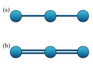
Figure 1: One-dimensional linear graph states of three qutrits. (a) A linear graph state in which both edges correspond to $CZ$ gates. (b) A linear graph state in which both edges correspond to $CZ^{2}$ gates.

With these ingredients in hand, our proposal for generating 1D linear photonic qutrit graph states comprised of only $CZ$ edges (as in Fig. 1(a)) from a quantum emitter with three ground levels is as follows:

• Prepare the emitter in the state $|0\rangle_{\text{e}}$.

• Perform a Hadamard gate $H$, Eq. (6), to produce the state $|X_{0}\rangle=|0\rangle_{\text{e}}+|1\rangle_{\text{e}}+|2\rangle_{\text{e}}$.

• Generate a time-bin encoded photon with a photon-pumping operation ${\cal P}_{\mathrm{pump}}$, Eq. (14), to obtain the state $\sum_{i=0}^{2}|i\rangle_{\text{e}}|i\rangle_{\text{p}_{1}}=|0\rangle_{\text{e}}|0\rangle_{\text{p}_{1}}+|1\rangle_{\text{e}}|1\rangle_{\text{p}_{1}}+|2\rangle_{\text{e}}|2\rangle_{\text{p}_{1}}$.

• Perform an $H$ gate on the emitter to obtain $\sum_{i,j=0}^{2}\omega^{ij}|j\rangle_{\text{e}}|i\rangle_{\text{p}_{1}}=|X_{0}\rangle_{\text{e}}|0\rangle_{\text{p}_{1}}+|X_{1}\rangle_{\text{e}}|1\rangle_{\text{p}_{1}}+|X_{2}\rangle_{\text{e}}|2\rangle_{\text{p}_{1}}$.

• Repeat steps 3 and 4 two more times to produce the state $\sum_{i,j,k,l=0}^{2}\omega^{ij}\omega^{jk}\omega^{kl}\,|l\rangle_{\text{e}}|k\rangle_{\text{p}_{3}}|j\rangle_{\text{p}_{2}}|i\rangle_{\text{p}_{1}}.$

• Measure the emitter in the $Z$ basis to decouple it from the photons. If the measurement outcome is 0, we obtain the photonic state $\sum_{i,j,k=0}^{2}\omega^{ij}\omega^{jk}\,|k\rangle_{\text{p}_{3}}|j\rangle_{\text{p}_{2}}|i\rangle_{\text{p}_{1}}$, and if the outcome is 1 (or 2), then performing a $Z^{2}$ (or $Z$) gate on photon 3 yields the same photonic state.

The final state is a 3-qutrit linear photonic graph state in which each edge corresponds to a $CZ$ operator, as in Fig. 1(a). By repeating steps 3 and 4 a total of $n$ times, one can produce a linear graph state of $n$ photonic qutrits.

How can we produce a state like that shown in Fig. 1(b)? In this state, each edge now corresponds to a $CZ^{2}$ gate. This state can be generated using a very similar protocol as the one above, except that we replace all but the first Hadamard gate by $H^{\dagger}$ gates:

• Prepare the emitter in the state $|0\rangle_{\text{e}}$.

• Perform a Hadamard gate $H$, Eq. (6), to produce the state $|X_{0}\rangle=|0\rangle_{\text{e}}+|1\rangle_{\text{e}}+|2\rangle_{\text{e}}$.

• Generate a time-bin encoded photon with a photon-pumping operation ${\cal P}_{\mathrm{pump}}$, Eq. (14), to obtain the state $\sum_{i=0}^{2}|i\rangle_{\text{e}}|i\rangle_{\text{p}_{1}}=|0\rangle_{\text{e}}|0\rangle_{\text{p}_{1}}+|1\rangle_{\text{e}}|1\rangle_{\text{p}_{1}}+|2\rangle_{\text{e}}|2\rangle_{\text{p}_{1}}$.

• Perform an $H^{\dagger}$ gate, Eq. (8), on the emitter to obtain $\sum_{i,j=0}^{2}\omega^{2ij}|j\rangle_{\text{e}}|i\rangle_{\text{p}_{1}}=|X_{0}\rangle_{\text{e}}|0\rangle_{\text{p}_{1}}+|X_{2}\rangle_{\text{e}}|1\rangle_{\text{p}_{1}}+|X_{1}\rangle_{\text{e}}|2\rangle_{\text{p}_{1}}$.

• Repeat steps 3 and 4 two more times to produce the state $\sum_{i,j,k,l=0}^{2}\omega^{2ij}\omega^{2jk}\omega^{2kl}\,|l\rangle_{\text{e}}|k\rangle_{\text{p}_{3}}|j\rangle_{\text{p}_{2}}|i\rangle_{\text{p}_{1}}$.

• Measure the emitter in the $Z$ basis to decouple it from the photons. If the measurement outcome is 0, we obtain the photonic state $\sum_{i,j,k=0}^{2}\omega^{2ij}\omega^{2jk}\,|k\rangle_{\text{e}}|j\rangle_{\text{p}_{2}}|i\rangle_{\text{p}_{1}}$, and if the outcome is 1 (or 2), then performing a $Z$ ($Z^{2}$) gate on photon 3 yields the same photonic state.

The final state in step 6 is a 3-photonic-qutrit linear graph state with $CZ^{2}$ edges, as in Fig. 1(b). Here also, repeating steps 3 and 4 a total of $n$ times yields an $n$-photon linear graph state with the same structure. Both of the above protocols can be straightforwardly generalized to the case of $q$-state photonic time-bin graph states generated from $q$-level quantum emitters.

IV AME state generation

Absolutely maximally entangled (AME) states, also referred to in some works as maximally multipartite entangled states Facchi [2009], Goyeneche et al. [2015], Raissi and Karimipour [2017], are pure $n$-qudit quantum states with local dimension $q$ such that every reduced density matrix on at most half the system size is maximally mixed. For example, the Bell state $|\phi^{+}\rangle=|00\rangle+|11\rangle$ and the GHZ state $|GHZ\rangle=|0000\rangle+|1111\rangle$ are both AME states because the reduced density matrices on each half of the system are completely mixed. More formally, an $\mathrm{AME}(n,q)$ state is a $n$-qudit pure state in $\operatorname{\mathcal{H}}(n,q)\coloneqq\mathbb{C}_{q}^{\otimes n}$ iff

$$\rho_{S}=\operatorname{\mathrm{Tr}}_{S^{c}}|\psi\rangle\langle\psi|\propto\mathbbm{1}\qquad\forall S\subset\{1,\ldots,n\},|S|\leq\left\lfloor n/2\right\rfloor\ ,$$

where $S^{c}$ denotes the complementary set of $S$. We denote an AME state by $|\mathrm{AME}(n,q)\rangle$. In this section, we describe how one can generate some of these states from quantum emitters.

IV.1 Generating AME states of $4$ qutrits

While it is known that AME states of $4$ qubits do not exist Scott [2004], Rains [1999], such states can exist for $q>2$ Helwig [2013], Raissi et al. [2018]. For example, in the case of 4 qutrits ($q=3$), the corresponding AME state can be written explicitly as Helwig [2013]:

$$|\mathrm{AME}(4,3)\rangle=\sum_{i,j=0}^{2}|i,j,i+j,i+2j\rangle\ .$$ (15)

This state is equivalent to the graph state representation shown in Fig. 2 Helwig [2013].

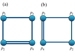
Figure 2: AME state of $4$ qutrits. (a) The graph that represents an $\mathrm{AME}(4,3)$ state. (b) A graph representing a state that is the same as the one in (a) up to a rearrangement of the qutrits.

In what follows, we present two protocols for generating this state from two quantum emitters, each of which has three ground levels, one of which is optically coupled to an excited state via a cyclic transition. The two protocols produce two states that are the same up to a swapping of two photonic qutrits. The gates we use in the first method (Fig. 2 (a)) are $CZ$ (Eq. (12)), $H$ (Eq. (6)), and $H^{\dagger}$ (Eq. (8)), and the gates we use in the second method (Fig. 2 (b)) are $CZ$ (Eq. (12)), $H$ (Eq. (6)), and $CZ^{2}$ (Eq. (13)). In both protocols, we make use of entangling operations between the emitters, in the spirit of Refs. Economou et al. [2010b], Buterakos et al. [2017], Russo et al. [2019b], Gimeno-Segovia et al. [2019b], Michaels et al. [2021], Hilaire et al. [2021], Li et al. [2022].

Here is the first method of generating an AME state of $4$ qutrits:

• Prepare the two emitters in the state $|0\rangle_{\text{e}_{1}}|0\rangle_{\text{e}_{2}}$.

• Perform a Hadamard gate $H$, Eq. (6), on each emitter to obtain the state $|X_{0}\rangle_{\text{e}_{1}}|X_{0}\rangle_{\text{e}_{2}}=\sum_{i,j=0}^{2}|i\rangle_{\text{e}_{1}}|j\rangle_{\text{e}_{2}}$.

• Perform a $CZ$ gate, Eq. (12), on the two emitters to obtain $\sum_{i,j=0}^{2}\omega^{ij}\ |i\rangle_{\text{e}_{1}}|j\rangle_{\text{e}_{2}}$.

• Perform photon-pumping operations ${\cal P}_{\mathrm{pump}}$, Eq. (14), on each emitter to produce time-bin encoded photons, yielding the state $\sum_{i,j=0}^{2}\omega^{ij}\ |i\rangle_{\text{e}_{1}}|i\rangle_{\text{p}_{1}}|j\rangle_{\text{e}_{2}}|j\rangle_{\text{p}_{2}}$.

• Perform an $H$ gate, Eq. (6), on the first emitter and an $H^{\dagger}$ gate, Eq. (8), on the second emitter to obtain $\sum_{i,j=0}^{2}\omega^{ij}|X_{i}\rangle_{\text{e}_{1}}|i\rangle_{\text{p}_{1}}|X_{2j\!\!\!\mod 3}\rangle_{\text{e}_{2}}|j\rangle_{\text{p}_{2}}=\sum_{i,j,k,l=0}^{2}\omega^{ij}\omega^{ik}\omega^{2jl}\ |k\rangle_{\text{e}_{1}}|i\rangle_{\text{p}_{1}}|l\rangle_{\text{e}_{2}}|j\rangle_{\text{p}_{2}}$.

• Perform a $CZ$ gate on the two emitters to produce the state $\sum_{i,j,k,l=0}^{2}\omega^{ij}\omega^{ik}\omega^{2jl}\omega^{kl}\ |k\rangle_{\text{e}_{1}}|i\rangle_{\text{p}_{1}}|l\rangle_{\text{e}_{2}}|j\rangle_{\text{p}_{2}}$.

• Perform photon-pumping operations ${\cal P}_{\mathrm{pump}}$ on each emitter to produce two more time-bin encoded photons, yielding the state $\sum_{i,j,k,l=0}^{2}\omega^{ij}\omega^{ik}\omega^{2jl}\omega^{kl}\ |k\rangle_{\text{e}_{1}}|k\rangle_{\text{p}_{3}}|i\rangle_{\text{p}_{1}}|l\rangle_{\text{e}_{2}}|l\rangle_{\text{p}_{4}}|j\rangle_{\text{p}_{2}}$.

• Perform an $H$ gate on each emitter and then measure each emitter in the $Z$ basis. Perform the local gates $Z_{\text{p}_{3}}^{2o_{1}}Z_{\text{p}_{4}}^{2o_{2}}$ on photons 3 and 4, where $o_{1}$ and $o_{2}$ are the measurement outcomes for emitters 1 and 2, respectively, to finally arrive at the state $\sum_{i,j,k,l=0}^{2}\omega^{ij}\omega^{ik}\omega^{2jl}\omega^{kl}\ |k\rangle_{\text{p}_{3}}|i\rangle_{\text{p}_{1}}|l\rangle_{\text{p}_{4}}|j\rangle_{\text{p}_{2}}$.

The final state in step 8 is the state $|\mathrm{AME}(4,3)\rangle$ shown in Fig. 2(a). This state is equivalent to Eq. (15); it can be obtained from that equation by applying Hadamard gates to the third and fourth qudits and by relabeling qutrits.

To produce the state shown in Fig. 2(b), we propose the following slightly modified protocol. The first 4 steps remain the same as above, but steps 5-8 are different:

• Perform a Hadamard gate $H$, Eq. (6), on each emitter to obtain the state $\sum_{i,j=0}^{2}\omega^{ij}\ |X_{i}\rangle_{\text{e}_{1}}|i\rangle_{\text{p}_{1}}|X_{j}\rangle_{\text{e}_{2}}|j\rangle_{\text{p}_{2}}=\sum_{i,j,k,l=0}^{2}\omega^{ij}\omega^{ik}\omega^{jl}\ |k\rangle_{\text{e}_{1}}|i\rangle_{\text{p}_{1}}|l\rangle_{\text{e}_{2}}|j\rangle_{\text{p}_{2}}$.

• Perform $CZ^{2}$, Eq. (13), on the two emitters, after which the state is $\sum_{i,j,k,l=0}^{2}\omega^{ij}\omega^{ik}\omega^{jl}\omega^{2kl}\ |k\rangle_{\text{e}_{1}}|i\rangle_{\text{p}_{1}}|l\rangle_{\text{e}_{2}}|j\rangle_{\text{p}_{2}}$.

• Perform photon-pumping operations ${\cal P}_{\mathrm{pump}}$, Eq. (14), on each emitter to produce two more time-bin encoded photons, yielding the state $\sum_{i,j,k,l=0}^{2}\omega^{ij}\omega^{ik}\omega^{jl}\omega^{2kl}\ |k\rangle_{\text{e}_{1}}|k\rangle_{\text{p}_{3}}|i\rangle_{\text{p}_{1}}|l\rangle_{\text{e}_{2}}|l\rangle_{\text{p}_{4}}|j\rangle_{\text{p}_{2}}$.

• Perform an $H$ gate on each emitter and then measure each emitter in the $Z$ basis. Perform the local gates $Z_{\text{p}_{3}}^{2o_{1}}Z_{\text{p}_{4}}^{2o_{2}}$ on photons 3 and 4, where $o_{1}$ and $o_{2}$ are the measurement outcomes for emitters 1 and 2, respectively, to finally arrive at the state $\sum_{i,j,k,l=0}^{2}\omega^{ij}\omega^{ik}\omega^{jl}\omega^{2kl}\ |k\rangle_{\text{p}_{3}}|i\rangle_{\text{p}_{1}}|l\rangle_{\text{p}_{4}}|j\rangle_{\text{p}_{2}}$.

The final state in step 8 is the state shown in Fig. 2(b). We see that we have the freedom to choose between performing a $CZ^{2}$ gate on the emitters or performing an $H^{\dagger}$ (instead of $H$) gate on one emitter followed by a $CZ$ gate on the two emitters. Note also that larger ladder-type qudit graph states with arbitrary combinations of $CZ$ and $CZ^{2}$ edges can be produced by repeating steps 3-6 in the above protocols.

IV.2 Generating AME states of $5$ qudits

AME states of $5$ qubits were shown to exist in Ref. Laflamme et al. [1996]. By exploiting a connection to quantum orthogonal arrays, explicit examples of $\mathrm{AME}(5,q)$ states for any local dimension $q\geq 2$ were discovered more recently Goyeneche et al. [2018]:

$$|\mathrm{AME}(5,q)\rangle=\sum_{i,j=0}^{q-1}|i,j,i+j\rangle|\phi_{i,j}\rangle\ ,$$ (16)

where $|\phi_{i,j}\rangle=X^{i}\otimes Z^{j}\sum_{\alpha=0}^{q-1}|\alpha,\alpha\rangle$. One can also show that this state has a graph representation. In particular, if one performs Hadamard gates on the third and fourth qudits, the resulting state is the graph state shown in Fig. 3.

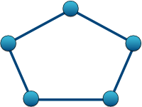
Figure 3: Graph representation of $\mathrm{AME}(5,q)$ states.

In this section we present two general protocols for generating such states that work for all values of the local dimension $q$. The first uses only a single quantum emitter but assumes the capability of re-interfering an emitted photon with the emitter. The second protocol does not require photon-emitter interference, but at the expense of needing two coupled quantum emitters. In both protocols, we assume the emitters have $q$ ground states, one of which can be optically excited to a higher-energy state via a cyclic transition. This allows for a photon-pumping operation analogous to Eq. (14).

We begin by presenting the protocol that requires only one quantum emitter with $q$ ground levels:

• Prepare the emitter in the state $|0\rangle_{\text{e}}$.

• Perform a Hadamard gate $H$, Eq. (6), to produce the state $|X_{0}\rangle=\sum_{i}|i\rangle_{\text{e}}$.

• Perform a photon-pumping operation ${\cal P}_{\mathrm{pump}}$, Eq. (14), to generate a time-bin encoded photon, yielding the state $\sum_{i=0}^{q-1}|i\rangle_{\text{e}}|i\rangle_{\text{p}_{1}}$.

• Perform an $H$ gate on the emitter to get $\sum_{i,j=0}^{q-1}\omega^{ij}\,|j\rangle_{\text{e}}|i\rangle_{\text{p}_{1}}$.

• Repeat steps 3 and 4 three more times to obtain $\sum_{i,j,k,l,m=0}^{q-1}\omega^{ij}\omega^{jk}\omega^{kl}\omega^{lm}\ |m\rangle_{\text{e}}|l\rangle_{\text{p}_{4}}|k\rangle_{\text{p}_{3}}|j\rangle_{\text{p}_{2}}|i\rangle_{\text{p}_{1}}$.

• Interfere the first photon $\text{p}_{1}$ with the emitter to perform a $CZ$ gate between them, yielding

  $$\sum_{i,j,k,l,m}\omega^{ij}\omega^{jk}\omega^{kl}\omega^{lm}\omega^{mi}|m\rangle_{\text{e}}|l\rangle_{\text{p}_{4}}|k\rangle_{\text{p}_{3}}|j\rangle_{\text{p}_{2}}|i\rangle_{\text{p}_{1}}.$$

• Perform a photon-pumping operation ${\cal P}_{\mathrm{pump}}$ followed by an $H$ gate on the emitter to obtain

  $$\sum_{i,j,k,l,m,r}\omega^{ij}\omega^{jk}\omega^{kl}\omega^{lm}\omega^{mi}\omega^{mr}|r\rangle_{\text{e}}|m\rangle_{\text{p}_{5}}|l\rangle_{\text{p}_{4}}|k\rangle_{\text{p}_{3}}|j\rangle_{\text{p}_{2}}|i\rangle_{\text{p}_{1}}.$$

• Measure the emitter in the $Z$ basis and perform $Z_{\text{p}_{5}}^{(q-1)o}$ on photon $\text{p}_{5}$, where $o$ is the measurement outcome. The resulting state is the desired AME state:

  $$\begin{split}&|\mathrm{AME}(5,q)\rangle=\\ &\sum_{i,j,k,l,m}\omega^{ij}\omega^{jk}\omega^{kl}\omega^{lm}\omega^{mi}|m\rangle_{\text{p}_{5}}|l\rangle_{\text{p}_{4}}|k\rangle_{\text{p}_{3}}|j\rangle_{\text{p}_{2}}|i\rangle_{\text{p}_{1}}.\end{split}$$

In the protocol described above, we need to re-interfere one of the emitted photons with the emitter to generate a $CZ$ gate between them. While several works have proposed schemes for doing this in the case photonic qubits Pichler et al. [2017], Zhan and Sun [2020], Wan et al. [2021], Shi and Waks [2021b], the analogous qudit operation may be substantially more challenging. This motivates the development of an alternative protocol that does not require such an operation. Such an alternative is possible if have access to two coupled emitters with $q$ ground levels each; one such protocol works as follows:

• Prepare the two emitters in the state $|0\rangle_{\text{e}_{1}}|0\rangle_{\text{e}_{2}}$.

• Perform a Hadamard gate $H$, Eq. (6), on each emitter, yielding $\sum_{i,j=0}^{q-1}|i\rangle_{\text{e}_{1}}|j\rangle_{\text{e}_{2}}$.

• Perform a $CZ$ gate, Eq. (5), on the two emitters to get $\sum_{i,j=0}^{q-1}\omega^{ij}\ |i\rangle_{\text{e}_{1}}|j\rangle_{\text{e}_{2}}$.

• Perform photon-pumping operations ${\cal P}_{\mathrm{pump}}$, Eq. (14), to each emitter to create two time-bin photonic qudits, yielding $\sum_{i,j=0}^{q-1}\omega^{ij}\ |i\rangle_{\text{e}_{1}}|i\rangle_{\text{p}_{1}}|j\rangle_{\text{e}_{2}}|j\rangle_{\text{p}_{2}}$.

• Perform an $H$ gate on each emitter to get $\sum_{i,j,k,l=0}^{q-1}\omega^{ij}\omega^{ik}\omega^{jl}\ |k\rangle_{\text{e}_{1}}|i\rangle_{\text{p}_{1}}|l\rangle_{\text{e}_{2}}|j\rangle_{\text{p}_{2}}$.

• Perform a photon-pumping operation on the first emitter ($\text{e}_{1}$) to produce another photon: $\sum_{i,j,k,l=0}^{q-1}\omega^{ij}\omega^{ik}\omega^{jl}\ |k\rangle_{\text{e}_{1}}|k\rangle_{\text{p}_{3}}|i\rangle_{\text{p}_{1}}|l\rangle_{\text{e}_{2}}|j\rangle_{\text{p}_{2}}$.

• Perform an $H$ gate on the first emitter ($\text{e}_{1}$) to get $\sum_{i,j,k,l=0}^{q-1}\omega^{ij}\omega^{ik}\omega^{jl}\omega^{km}\ |m\rangle_{\text{e}_{1}}|k\rangle_{\text{p}_{3}}|i\rangle_{\text{p}_{1}}|l\rangle_{\text{e}_{2}}|j\rangle_{\text{p}_{2}}$.

• Perform a $CZ$ gate on the two emitters to get

  $$\sum_{\begin{subarray}{c}i,j,k,\\ l,m=0\end{subarray}}^{q-1}\omega^{ij}\omega^{ik}\omega^{jl}\omega^{km}\omega^{ml}\ |m\rangle_{\text{e}_{1}}|k\rangle_{\text{p}_{3}}|i\rangle_{\text{p}_{1}}|l\rangle_{\text{e}_{2}}|j\rangle_{\text{p}_{2}}.$$

• Perform a photon-pumping operation on each emitter, followed by an $H$ gate on each emitter:

  $$\sum_{\begin{subarray}{c}i,j,k,l\\ m,r,s=0\end{subarray}}^{q-1}\Omega|r\rangle_{\text{e}_{1}}|m\rangle_{\text{p}_{4}}|k\rangle_{\text{p}_{3}}|i\rangle_{\text{p}_{1}}|s\rangle_{\text{e}_{2}}|l\rangle_{\text{p}_{5}}|j\rangle_{\text{p}_{2}},$$

  where $\Omega=\omega^{ij}\omega^{ik}\omega^{jl}\omega^{km}\omega^{ml}\omega^{mr}\omega^{ls}$.

• Measure both emitters in the $Z$ basis and perform $Z_{\text{p}_{4}}^{(q-1)o_{1}}Z_{\text{p}_{5}}^{(q-1)o_{2}}$ on photons $\text{p}_{4}$ and $\text{p}_{5}$, where $o_{1}$ and $o_{2}$ are the measurement outcomes. This yields the desired 5-photon state:

  $$\begin{split}&|\mathrm{AME}(5,q)\rangle=\\ &\sum_{\begin{subarray}{c}i,j,k,\\ l,m=0\end{subarray}}^{q-1}\omega^{ij}\omega^{ik}\omega^{jl}\omega^{km}\omega^{ml}\ |m\rangle_{\text{p}_{5}}|k\rangle_{\text{p}_{3}}|i\rangle_{\text{p}_{1}}|l\rangle_{\text{p}_{4}}|j\rangle_{\text{p}_{2}}.\end{split}$$

IV.3 Generating AME states of $6$ qudits

Next, we consider $\mathrm{AME}(6,q)$ states. The graph representations of two such states are shown in Fig. 4 Helwig [2013], Cervera-Lierta et al. [2019]. Here, we present protocols for generating both of these types of graph states for qudits of arbitrary local dimension $q$. The first protocol utilizes two coupled emitters with $q$ ground levels each and photon-emitter interference to generate graph states of the sort shown in Fig. 4(a). The protocol consists of the following steps:

• Prepare two $q$-level emitters in the state $|0\rangle_{\text{e}_{1}}|0\rangle_{\text{e}_{2}}$.

• Perform a Hadamard gate $H$, Eq. (6), on each emitter to obtain $\sum_{i,j=0}^{q-1}|i\rangle_{\text{e}_{1}}|j\rangle_{\text{e}_{2}}$.

• Perform a $CZ$ gate, Eq. (5), on the two emitters to get $\sum_{i,j=0}^{q-1}\omega^{ij}\ |i\rangle_{\text{e}_{1}}|j\rangle_{\text{e}_{2}}$.

• Perform photon-pumping operations ${\cal P}_{\mathrm{pump}}$, Eq. (14), on each emitter to produce two photons: $\sum_{i,j=0}^{q-1}\omega^{ij}\ |i\rangle_{\text{e}_{1}}|i\rangle_{\text{p}_{1}}|j\rangle_{\text{e}_{2}}|j\rangle_{\text{p}_{2}}$.

• Perform an $H$ gate on each emitter to obtain $\sum_{i,j,k,l=0}^{q-1}\omega^{ij}\omega^{ik}\omega^{jl}\ |k\rangle_{\text{e}_{1}}|i\rangle_{\text{p}_{1}}|l\rangle_{\text{e}_{2}}|j\rangle_{\text{p}_{2}}$.

• Apply two $CZ$ gates, one on the first photon ($\text{p}_{1}$) and the second emitter ($\text{e}_{2}$), and the other on the two emitters, yielding $\sum_{i,j,k,l=0}^{q-1}\omega^{ij}\omega^{ik}\omega^{jl}\omega^{il}\omega^{kl}\ |k\rangle_{\text{e}_{1}}|i\rangle_{\text{p}_{1}}|l\rangle_{\text{e}_{2}}|j\rangle_{\text{p}_{2}}$.

• Perform photon-pumping operations on each emitter to create two more photons: $\sum_{i,j,k,l}\omega^{ij}\omega^{ik}\omega^{jl}\omega^{il}\omega^{kl}\ |k\rangle_{\text{e}_{1}}|k\rangle_{\text{p}_{3}}|i\rangle_{\text{p}_{1}}|l\rangle_{\text{e}_{2}}|l\rangle_{\text{p}_{4}}|j\rangle_{\text{p}_{2}}$.

• Perform an $H$ gate on each emitter to get $\sum_{\begin{subarray}{c}i,j,k,\\ l,m,r\end{subarray}}\Omega\ |m\rangle_{\text{e}_{1}}|k\rangle_{\text{p}_{3}}|i\rangle_{\text{p}_{1}}|r\rangle_{\text{e}_{2}}|l\rangle_{\text{p}_{4}}|j\rangle_{\text{p}_{2}}$, where $\Omega\coloneqq\omega^{ij}\omega^{ik}\omega^{jl}\omega^{il}\omega^{kl}\omega^{km}\omega^{lr}$.

• Perform three $CZ$ gates: One $CZ$ on $\text{p}_{4}$ and $\text{e}_{1}$, the other $CZ$ on $\text{p}_{2}$ and $\text{e}_{2}$, and the third $CZ$ operator on $\text{e}_{1}$ and $\text{e}_{2}$. With this we obtain

  $$\sum_{\begin{subarray}{c}i,j,k,\\ l,m,r=0\end{subarray}}^{q-1}\Omega^{\prime}\ |m\rangle_{\text{e}_{1}}|k\rangle_{\text{p}_{3}}|i\rangle_{\text{p}_{1}}|r\rangle_{\text{e}_{2}}|l\rangle_{\text{p}_{4}}|j\rangle_{\text{p}_{2}},$$

  where $\Omega^{\prime}\coloneqq\omega^{ij}\omega^{ik}\omega^{jl}\omega^{il}\omega^{kl}\omega^{km}\omega^{lr}\omega^{lm}\omega^{jr}\omega^{mr}$.

• Perform a photon-pumping operation on each emitter, followed by an $H$ gate on each emitter. Measure both emitters and perform the gates $Z_{\text{p}_{5}}^{(q-1)o_{1}}Z_{\text{p}_{6}}^{(q-1)o_{2}}$ on the newly generated photons $\text{p}_{5}$ and $\text{p}_{6}$, where $o_{1}$ and $o_{2}$ are the measurement outcomes. The final state is

  $$\begin{split}&|\mathrm{AME}(6,q)\rangle=\\ &\sum_{\begin{subarray}{c}i,j,k,\\ l,m,r=0\end{subarray}}^{q-1}\Omega^{\prime}\ |m\rangle_{\text{p}_{5}}|k\rangle_{\text{p}_{3}}|i\rangle_{\text{p}_{1}}|r\rangle_{\text{p}_{6}}|l\rangle_{\text{p}_{4}}|j\rangle_{\text{p}_{2}},\end{split}$$

  which is the one shown in Fig. 4(a).

We now present a protocol for generating the $\mathrm{AME}(6,q)$ states corresponding to the graph shown in Fig. 4(b). This protocol requires three coupled emitters with $q$ ground levels each but does not need photon-emitter interference:

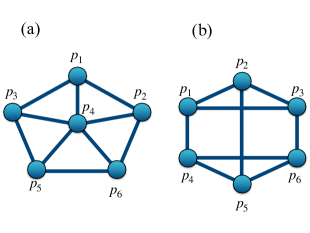
Figure 4: Two types of $\mathrm{AME}(6,q)$ states represented as graphs.

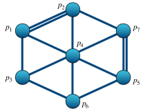
Figure 5: Graph representing the $\mathrm{AME}(7,3)$ state.

• Prepare three emitters in the state $|0\rangle_{\text{e}_{1}}|0\rangle_{\text{e}_{2}}|0\rangle_{\text{e}_{3}}$.

• Perform a Hadamard gate $H$, Eq. (6), on each emitter to obtain $\sum_{i,j,k=0}^{q-1}|i\rangle_{\text{e}_{1}}|j\rangle_{\text{e}_{2}}|k\rangle_{\text{e}_{3}}$.

• Perform three $CZ$ gates on each pair of emitters (i.e., on $\text{e}_{1}$ and $\text{e}_{2}$, on $\text{e}_{2}$ and $\text{e}_{3}$, and on $\text{e}_{1}$ and $\text{e}_{3}$): $\sum_{i,j,k=0}^{q-1}\omega^{ij}\omega^{jk}\omega^{ik}\ |i\rangle_{\text{e}_{1}}|j\rangle_{\text{e}_{2}}|k\rangle_{\text{e}_{3}}$.

• Perform photon-pumping operations ${\cal P}_{\mathrm{pump}}$, Eq. (14), to each emitter to create three photons: $\sum_{i,j,k=0}^{q-1}\omega^{ij}\omega^{jk}\omega^{ik}\ |i\rangle_{\text{e}_{1}}|i\rangle_{\text{p}_{1}}|j\rangle_{\text{e}_{2}}|j\rangle_{\text{p}_{2}}|k\rangle_{\text{e}_{3}}|k\rangle_{\text{p}_{3}}$.

• Perform an $H$ gate on each emitter: $\sum_{i,j,k,l,m,r=0}^{q-1}\Theta\ |l\rangle_{\text{e}_{1}}|i\rangle_{\text{p}_{1}}|m\rangle_{\text{e}_{2}}|j\rangle_{\text{p}_{2}}|r\rangle_{\text{e}_{3}}|k\rangle_{\text{p}_{3}}$, where $\Theta\coloneqq\omega^{ij}\omega^{jk}\omega^{ik}\omega^{il}\omega^{jm}\omega^{kr}$.

• Again perform a $CZ$ gate on each pair of emitters:

  $$\sum_{i,j,k,l,m,r=0}^{q-1}\Theta^{\prime}\ |l\rangle_{\text{e}_{1}}|i\rangle_{\text{p}_{1}}|m\rangle_{\text{e}_{2}}|j\rangle_{\text{p}_{2}}|r\rangle_{\text{e}_{3}}|k\rangle_{\text{p}_{3}},$$

  where $\Theta^{\prime}\coloneqq\omega^{ij}\omega^{jk}\omega^{ik}\omega^{il}\omega^{jm}\omega^{kr}\omega^{lm}\omega^{mr}\omega^{lr}$.

• Perform a photon-pumping operation on each emitter, followed by an $H$ gate on each emitter. Measure all three emitters and perform the gates $Z_{\text{p}_{4}}^{(q-1)o_{1}}Z_{\text{p}_{5}}^{(q-1)o_{2}}Z_{\text{p}_{6}}^{(q-1)o_{3}}$ on the newly generated photons $\text{p}_{4}$, $\text{p}_{5}$, and $\text{p}_{6}$, where $o_{1}$, $o_{2}$, $o_{3}$ are the measurement outcomes. The final state is

  $$\begin{split}&|\mathrm{AME}(6,q)\rangle=\\ &\sum_{i,j,k,l,m,r=0}^{q-1}\Theta^{\prime}\ |l\rangle_{\text{p}_{4}}|i\rangle_{\text{p}_{1}}|m\rangle_{\text{p}_{5}}|j\rangle_{\text{p}_{2}}|r\rangle_{\text{p}_{6}}|k\rangle_{\text{p}_{3}},\end{split}$$

  which is the one shown in Fig. 4(b).

IV.4 Generating AME states of $7$ qutrits

It is known that while AME states of $7$ qubits do not exist Huber et al. [2017], AME states of $7$ qutrits do exist. Through an exhaustive numerical search checking the bipartite entanglement of various graph states, it was found that the graph shown in Fig. 5 corresponds to the $\mathrm{AME}(7,3)$ state Helwig [2013]. In this section, we show how to generate this state. Our protocol uses two quantum emitters with three ground levels each, as well as photon-emitter interference. The protocol is similar to the one presented above for the AME(6,$q$) states depicted in Fig. 4 due to the similarity in graph structure.

• Prepare the two quantum emitters in the state $|0\rangle_{\text{e}_{1}}|0\rangle_{\text{e}_{2}}$.

• Perform a Hadamard gate $H$, Eq. (6), on each emitter: $|X_{0}\rangle_{\text{e}_{1}}|X_{0}\rangle_{\text{e}_{2}}=\sum_{i,j=0}^{2}|i\rangle_{\text{e}_{1}}|j\rangle_{\text{e}_{2}}$.

• Perform $CZ^{2}$, Eq. (13), on the two emitters to get $\sum_{i,j=0}^{2}\omega^{2ij}\ |i\rangle_{\text{e}_{1}}|j\rangle_{\text{e}_{2}}$.

• Perform the photon-pumping operation ${\cal P}_{\mathrm{pump}}$, Eq. (14), on each emitter to create two photons: $\sum_{i,j=0}^{2}\omega^{2ij}\ |i\rangle_{\text{e}_{1}}|i\rangle_{\text{p}_{1}}|j\rangle_{\text{e}_{2}}|j\rangle_{\text{p}_{2}}$.

• Perform an $H$ gate on each emitter: $\sum_{i,j,k,l=0}^{2}\omega^{2ij}\omega^{ik}\omega^{jl}\ |k\rangle_{\text{e}_{1}}|i\rangle_{\text{p}_{1}}|l\rangle_{\text{e}_{2}}|j\rangle_{\text{p}_{2}}$.

• Apply two $CZ$ gates, Eq. (12), one on the first photon ($\text{p}_{1}$) and the second emitter ($\text{e}_{2}$), and the other on the two emitters ($\text{e}_{1}$ and $\text{e}_{2}$), yielding $\sum_{i,j,k,l=0}^{2}\omega^{2ij}\omega^{ik}\omega^{jl}\omega^{il}\omega^{kl}\ |k\rangle_{\text{e}_{1}}|i\rangle_{\text{p}_{1}}|l\rangle_{\text{e}_{2}}|j\rangle_{\text{p}_{2}}$.

• Perform photon-pumping operations on each emitter to create two more photons: $\sum_{\begin{subarray}{c}i,j,\\ k,l\end{subarray}}\omega^{2ij}\omega^{ik}\omega^{jl}\omega^{il}\omega^{kl}\ |k\rangle_{\text{e}_{1}}|k\rangle_{\text{p}_{3}}|i\rangle_{\text{p}_{1}}|l\rangle_{\text{e}_{2}}|l\rangle_{\text{p}_{4}}|j\rangle_{\text{p}_{2}}$.

• Perform an $H$ gate on each emitter: $\sum_{\begin{subarray}{c}i,j,k,\\ l,m,r=0\end{subarray}}^{2}\Xi\ |m\rangle_{\text{e}_{1}}|k\rangle_{\text{p}_{3}}|i\rangle_{\text{p}_{1}}|r\rangle_{\text{e}_{2}}|l\rangle_{\text{p}_{4}}|j\rangle_{\text{p}_{2}}$, where $\Xi\coloneqq\omega^{2ij}\omega^{ik}\omega^{jl}\omega^{il}\omega^{kl}\omega^{km}\omega^{lr}$.

• Perform two $CZ$ gates, one on $\text{p}_{4}$ and $\text{e}_{1}$, the other on $\text{e}_{1}$ and $\text{e}_{2}$, yielding $\sum_{\begin{subarray}{c}i,j,k,\\ l,m,r=0\end{subarray}}^{2}\Xi^{\prime}\ |m\rangle_{\text{e}_{1}}|k\rangle_{\text{p}_{3}}|i\rangle_{\text{p}_{1}}|r\rangle_{\text{e}_{2}}|l\rangle_{\text{p}_{4}}|j\rangle_{\text{p}_{2}}$ where $\Xi^{\prime}\coloneqq\omega^{2ij}\omega^{ik}\omega^{jl}\omega^{il}\omega^{kl}\omega^{km}\omega^{lr}\omega^{lm}\omega^{mr}$.

• Perform a photon-pumping operation on only $\text{e}_{2}$ to create one more photon: $\sum_{\begin{subarray}{c}i,j,k,\\ l,m,r=0\end{subarray}}^{2}\Xi^{\prime}\ |m\rangle_{\text{e}_{1}}|k\rangle_{\text{p}_{3}}|i\rangle_{\text{p}_{1}}|r\rangle_{\text{e}_{2}}|r\rangle_{\text{p}_{5}}|l\rangle_{\text{p}_{4}}|j\rangle_{\text{p}_{2}}$.

• Perform an $H^{\dagger}$ gate, Eq. (8), on $\text{e}_{2}$ to yield $\sum_{\begin{subarray}{c}i,j,k,l\\ m,r,s=0\end{subarray}}^{2}\Xi^{\prime\prime}\ |m\rangle_{\text{e}_{1}}|k\rangle_{\text{p}_{3}}|i\rangle_{\text{p}_{1}}|s\rangle_{\text{e}_{2}}|r\rangle_{\text{p}_{5}}|l\rangle_{\text{p}_{4}}|j\rangle_{\text{p}_{2}}$ where $\Xi^{\prime\prime}\coloneqq\omega^{2ij}\omega^{ik}\omega^{jl}\omega^{il}\omega^{kl}\omega^{km}\omega^{lr}\omega^{lm}\omega^{mr}\omega^{2sr}$.

• Apply two $CZ$ gates, one on the fourth photon ($\text{p}_{4}$) and the second emitter ($\text{e}_{2}$), and the other on $\text{p}_{2}$ and $\text{e}_{2}$:

  $$\sum_{\begin{subarray}{c}i,j,k,l\\ m,r,s=0\end{subarray}}^{2}\tilde{\Xi}\ |m\rangle_{\text{e}_{1}}|k\rangle_{\text{p}_{3}}|i\rangle_{\text{p}_{1}}|s\rangle_{\text{e}_{2}}|r\rangle_{\text{p}_{5}}|l\rangle_{\text{p}_{4}}|j\rangle_{\text{p}_{2}}.$$

  where

  $$\tilde{\Xi}\coloneqq\omega^{2ij}\omega^{ik}\omega^{jl}\omega^{il}\omega^{kl}\omega^{km}\omega^{lr}\omega^{lm}\omega^{mr}\omega^{2sr}\omega^{sl}\omega^{js}.$$

• Perform a photon-pumping operation on each emitter, followed by an $H$ gate on each emitter. Measure both emitters in the $Z$ basis and perform the gates $Z_{\text{p}_{6}}^{(q-1)o_{1}}Z_{\text{p}_{7}}^{(q-1)o_{2}}$ on the newly generated photons, $\text{p}_{6}$ and $\text{p}_{7}$, where $o_{1}$ and $o_{2}$ are the measurement outcomes. The final state is

  $$\begin{split}&|\mathrm{AME}(7,3)\rangle=\\ &\sum_{\begin{subarray}{c}i,j,k,l\\ m,r,s=0\end{subarray}}^{2}\tilde{\Xi}\ |m\rangle_{\text{p}_{6}}|k\rangle_{\text{p}_{3}}|i\rangle_{\text{p}_{1}}|s\rangle_{\text{p}_{7}}|r\rangle_{\text{p}_{5}}|l\rangle_{\text{p}_{4}}|j\rangle_{\text{p}_{2}},\end{split}$$

  which is the state shown in Fig. 5.

Graph	# photons	Local dimension	# emitters	Photon interference required?
	$n\geq 2$	$q\geq 2$	1	no
	$n=4$	$q=3$	2	no
	$n=5$	$q\geq 2$	First method: 1   Second method: 2	yes   no
	$n=6$	$q\geq 2$	2	yes
	$n=6$	$q\geq 2$	3	no
	$n=7$	$q=3$	2	yes

Table 1: Summary of the generation protocols of various multi-photon qudit graph states presented in this work. For each protocol, the corrsponding graph representation of the target state is shown, along with the number of photons it contains, the number $q$ of photonic time-bin states, the number of quantum emitters (with $q$ levels each) needed to produce the state, and whether or not photon-emitter interference is required for the protocol.

A summary of the multi-qudit graph states generation protocols presented so far is given in Table. 1.

V Quantum error correcting codes

It is known that AME states are useful for constructing QECCs Scott [2004], Raissi et al. [2018], Raissi [2020]. In this section, we show how this connection can be exploited to develop protocols for generating multiphoton logical states of QECCs. First, we briefly review the relation between certain QECCs and AME states. A subspace $\mathcal{C}$ spanned by an orthonormal set of states $\{|\psi_{0}\rangle,|\psi_{1}\rangle,\dots,|\psi_{q^{k}-1}\rangle\}$, also called codewords, is a QECC with parameters $[\![n,k,d]\!]_{q}$. This code is a $q^{k}$ dimensional subspace that encodes $k$ logical qudits into $n$ physical qudits, if it obeys the Knill-Laflamme conditions Knill and Laflamme [1997], Gottesman [1997]

$$\forall m,m^{\prime}\in[q^{k}]\colon\ \langle\psi_{m}|E^{\dagger}F|\psi_{m^{\prime}}\rangle=f(E^{\dagger}F)\,\delta_{m,m^{\prime}},$$ (17)

for all errors $E,F$ with $\text{weight}(E^{\dagger}F)\leq d$, where the weight of an operator is defined to be the number of sites on which it acts non-trivially. The parameter $d$ is the distance of the quantum code, which is the minimal number of single-qudit operations that are needed to create a non-zero overlap between any two codewords from the code state space $\mathcal{C}$. A QECC with minimum distance $d$ can correct errors that affect no more than $(d-1)/2$ of the physical qudits. In this section, we show how to generate a $[\![3,1,2]\!]_{3}$ QECC, for which the codewords are all AME states of $3$ qutrits.

First, let us review how to construct the $[\![3,1,2]\!]_{3}$ quantum code (see also Calderbank et al. [1998], Ketkar et al. [2006], Raissi [2020]). It is known that the $\mathrm{AME}(3,3)$ states Alsina and Razavi [2021], Raissi [2020]

$$\begin{split}|\psi_{0}\rangle&=\sum_{j=0}^{2}|j,j,j\rangle,\\ |\psi_{1}\rangle&=M|\psi_{0}\rangle=\sum_{j=0}^{2}|j+1,j,j+2\rangle,\\ |\psi_{2}\rangle&=M^{2}|\psi_{0}\rangle=\sum_{j=0}^{2}|j+2,j,j+1\rangle,\end{split}$$ (18)

are the codewords of the $[\![3,1,2]\!]_{3}$ code. In the above, the operator $M$ is defined as $M=X\otimes\mathbbm{1}\otimes X^{2}$.

In order to construct the corresponding graph states, it helps to first notice that by performing an $H$ gate, Eq. (6), on the first and third qudits, we get

$$|\psi^{\prime}_{0}\rangle=H\otimes\mathbbm{1}\otimes H\,|\psi_{0}\rangle=\sum_{i,j,k=0}^{2}\omega^{kj}\omega^{ij}\ |k,j,i\rangle,$$ (19)

$$|\psi^{\prime}_{1}\rangle=H\otimes\mathbbm{1}\otimes H\,|\psi_{1}\rangle=\sum_{i,j,k=0}^{2}\omega^{(j+1)k}\omega^{(j+2)i}\ |k,j,i\rangle,$$ (20)

$$|\psi^{\prime}_{2}\rangle=H\otimes\mathbbm{1}\otimes H\,|\psi_{2}\rangle=\sum_{i,j,k=0}^{2}\omega^{(j+2)k}\omega^{(j+1)i}\ |k,j,i\rangle\,.$$ (21)

Notice that the state $|\psi^{\prime}_{0}\rangle$ is equivalent to the 3-qutrit graph state shown in Fig. 1(a) and discussed in Sec. III. Thus, we already know how to generate this state, and so it remains to show how to produce $|\psi^{\prime}_{1}\rangle$ and $|\psi^{\prime}_{2}\rangle$ from a 3-level quantum emitter. For this, let us first discuss how to generate $|\psi^{\prime}_{1}\rangle$:

• Prepare the emitter in the state $|2\rangle_{\text{e}}$.

• Perform a Hadamard gate $H$, Eq. (6), to produce the state $|X_{2}\rangle_{\text{e}}=\sum_{i=0}^{2}\omega^{2i}|i\rangle_{\text{e}}=|0\rangle_{\text{e}}+\omega^{2}|1\rangle_{\text{e}}+\omega|2\rangle_{\text{e}}$.

• Generate a time-bin encoded photon with a photon-pumping operation ${\cal P}_{\mathrm{pump}}$, Eq. (14), to obtain the state $\sum_{i=0}^{2}\omega^{2i}|i\rangle_{\text{e}}|i\rangle_{\text{p}_{1}}=|0\rangle_{\text{e}}|0\rangle_{\text{p}_{1}}+\omega^{2}|1\rangle_{\text{e}}|1\rangle_{\text{p}_{1}}+\omega|2\rangle_{\text{e}}|2\rangle_{\text{p}_{1}}$.

• Perform an $H$ gate, Eq. (6), on the emitter to obtain $\sum_{i,j=0}^{2}\omega^{2i}\omega^{ij}|j\rangle_{\text{e}}|i\rangle_{\text{p}_{1}}=|X_{0}\rangle_{\text{e}}|0\rangle_{\text{p}_{1}}+\omega^{2}|X_{1}\rangle_{\text{e}}|1\rangle_{\text{p}_{1}}+\omega|X_{2}\rangle_{\text{e}}|2\rangle_{\text{p}_{1}}$.

• Repeat steps 3 and 4 to produce the state $\sum_{i,j,k=0}^{2}\omega^{2i}\omega^{ij}\omega^{jk}\,|k\rangle_{\text{e}}|j\rangle_{\text{p}_{2}}|i\rangle_{\text{p}_{1}}$.

• Perform a $Z$ gate, Eq. (2), on the emitter to obtain $\sum_{i,j,k=0}^{2}\omega^{2i}\omega^{ij}\omega^{jk}\omega^{k}\,|k\rangle_{\text{e}}|j\rangle_{\text{p}_{2}}|i\rangle_{\text{p}_{1}}$.

• Repeat steps 3 and 4 once more to produce the state $\sum_{i,j,k,l=0}^{2}\omega^{2i}\omega^{ij}\omega^{jk}\omega^{k}\omega^{kl}\,|l\rangle_{\text{e}}|k\rangle_{\text{p}_{3}}|j\rangle_{\text{p}_{2}}|i\rangle_{\text{p}_{1}}$.

• Measure the emitter in the $Z$ basis and perform the gate $Z_{\text{p}_{3}}^{2o}$ on photon $\text{p}_{3}$, where $o$ is the measurement outcome. The resulting state is the desired $|\psi^{\prime}_{1}\rangle$:

  $$|\psi^{\prime}_{1}\rangle=\sum_{i,j,k=0}^{2}\omega^{2i}\omega^{ij}\omega^{jk}\omega^{k}\,|k\rangle_{\text{p}_{3}}|j\rangle_{\text{p}_{2}}|i\rangle_{\text{p}_{1}}\ .$$ (22)

A similar protocol can be used to generate $|\psi^{\prime}_{2}\rangle$:

• Prepare the emitter in the state $|1\rangle_{\text{e}}$.

• Perform a Hadamard gate $H$, Eq. (6), to produce the state $|X_{1}\rangle_{\text{e}}=\sum_{i=0}^{2}\omega^{i}|i\rangle_{\text{e}}=|0\rangle_{\text{e}}+\omega|1\rangle_{\text{e}}+\omega^{2}|2\rangle_{\text{e}}$.

• Generate a time-bin encoded photon with a photon-pumping operation ${\cal P}_{\mathrm{pump}}$, Eq. (14), to obtain the state $\sum_{i=0}^{2}\omega^{i}|i\rangle_{\text{e}}|i\rangle_{\text{p}_{1}}=|0\rangle_{\text{e}}|0\rangle_{\text{p}_{1}}+\omega|1\rangle_{\text{e}}|1\rangle_{\text{p}_{1}}+\omega^{2}|2\rangle_{\text{e}}|2\rangle_{\text{p}_{1}}$.

• Perform an $H$ gate, Eq. (6), on the emitter to obtain $\sum_{i,j=0}^{2}\omega^{i}\omega^{ij}|j\rangle_{\text{e}}|i\rangle_{\text{p}_{1}}=|X_{0}\rangle_{\text{e}}|0\rangle_{\text{p}_{1}}+\omega|X_{1}\rangle_{\text{e}}|1\rangle_{\text{p}_{1}}+\omega^{2}|X_{2}\rangle_{\text{e}}|2\rangle_{\text{p}_{1}}$.

• Repeat steps 3 and 4 to produce the state $\sum_{i,j,k=0}^{2}\omega^{i}\omega^{ij}\omega^{jk}\,|k\rangle_{\text{e}}|j\rangle_{\text{p}_{2}}|i\rangle_{\text{p}_{1}}$.

• Perform a $Z^{2}$ gate, Eq. (4), on the emitter to obtain $\sum_{i,j,k=0}^{2}\omega^{i}\omega^{ij}\omega^{jk}\omega^{2k}\,|k\rangle_{\text{e}}|j\rangle_{\text{p}_{2}}|i\rangle_{\text{p}_{1}}$.

• Repeat steps 3 and 4 once more to produce the state $\sum_{i,j,k,l=0}^{2}\omega^{i}\omega^{ij}\omega^{jk}\omega^{2k}\omega^{kl}\,|l\rangle_{\text{e}}|k\rangle_{\text{p}_{3}}|j\rangle_{\text{p}_{2}}|i\rangle_{\text{p}_{1}}$.

• Measure the emitter in the $Z$ basis and perform the gate $Z_{\text{p}_{3}}^{2o}$ on photon $\text{p}_{3}$, where $o$ is the measurement outcome. The resulting state us the desired $|\psi^{\prime}_{2}\rangle$:

  $$|\psi^{\prime}_{2}\rangle=\sum_{i,j,k=0}^{2}\omega^{i}\omega^{ij}\omega^{jk}\omega^{2k}\,|k\rangle_{\text{p}_{3}}|j\rangle_{\text{p}_{2}}|i\rangle_{\text{p}_{1}}\ .$$ (23)

Similar protocols can be devised to generate the codewords of QECCs associated with any of the AME states discussed in Sec. IV.

VI Physical implementations

Photonic qudit states can be generated from a range of different emitters. On the solid-state side, an example is the well-known NV center in diamond, where among its three ground states, $|0\rangle$ and $|\pm 1\rangle$, state $|0\rangle$ can be reliably pumped to an excited state that subsequently decays back down to $|0\rangle$, emitting a photon Doherty et al. [2013], Wolfowicz et al. [2021]. NV centers can thus be used to generate photonic time-bin qutrits. Since however the NV has a very low probability of emitting into the zero-phonon line, it may be preferable to consider alternative defects. The silicon-carbon divacancy in SiC is another defect that has a triplet ground state, and that generally resembles the electronic structure of NV-diamond, but with improved optical properties and comparably long coherence times Christle et al. [2015]. For local dimension $q=4$, the silicon vacancy could be used instead.

Atomic systems provide even more options for the value of $q$, as they can contain well-resolved hyperfine states. Trapped ions such as $\ce{{}^{40}Ca+}$ Ringbauer et al. [2022] and $\ce{{}^{171}Yb+}$ Timoney et al. [2011], Webster et al. [2013], Aksenov et al. [2022] can serve as multi-level quantum emitters with local dimensions ranging from $q=3$ up to $q=7$ Timoney et al. [2011], Webster et al. [2013], Randall et al. [2015], Senko et al. [2015], Ringbauer et al. [2022], Aksenov et al. [2022]. There has been significant experimental progress in realizing single- and multi-qudit gate operations in chains of such ions Ringbauer et al. [2022], Aksenov et al. [2022]. Few-atom systems in a cavity are another contender for generation of qudit graph states. A recent milestone experiment demonstrated the generation of GHZ and linear cluster states of qubits from a Rb atom Thomas et al. [2022]. While in that experiment the photonic qubit was encoded in the polarization degree of freedom, and therefore only two of the states in the ground state manifold were used explicitly in the protocol, a similar setup could be employed to demonstrate qudit graph-state generation with time-bin encoding and with more levels participating in generation process (up to $q=8$ when both the $F=1$ and the $F=2$ manifolds are used). To create more complex qudit graphs, cavity-mediated interactions between two or more atoms can be leveraged to create qudit CZ-type gates by modifying the protocol for the already demonstrated two-qubit gates in such systems Welte et al. [2018].

VII Conclusions and outlook

In conclusion, we presented explicit protocols for using coupled, controllable quantum emitters to deterministically generate multi-photon entangled states of time-bin qudits. Although our methods are quite general, we focused primarily on the problem of generating highly entangled states known as AME states, which are important for a number applications in quantum networks and quantum error correction. We showed that such states can be produced from a small number of emitters, with or without photon-emitter interference, provided emitters with the appropriate level structure are available. In some cases, we found that one less emitter can be used if photon-emitter interference is available, providing hints at what sort of resource tradeoffs are possible. Potential candidates include defect centers in solids as well as atomic systems. Our results provide a clear path forward toward the efficient generation of complex states of light for quantum information applications and a guide to experimental groups.

Future directions this work opens include addressing the question of what the minimal resources are—in terms of the number of emitters and the circuit depth—for the generation of a target qudit graph. Similar to the formalism developed to answer these questions in the context of qubits Li et al. [2022], one could set up a similar approach for qudits. Another interesting direction would be to design specific qudit gates for various candidate emitters and to quantify the anticipated performance of the protocols. Our protocols could also be combined with new approaches to photonic one-way quantum repeaters based on photonic qudit states Zheng et al. [2022] to build error-correction into that approach.