RNTrajRec: Road Network Enhanced Trajectory Recovery with Spatial-Temporal Transformer (Extended Version)

Abstract

GPS trajectories are the essential foundations for many trajectory-based applications, such as travel time estimation, traffic prediction and trajectory similarity measurement. Most applications require a large number of high sample rate trajectories to achieve a good performance. However, many real-life trajectories are collected with low sample rate due to energy concern or other constraints. We study the task of trajectory recovery in this paper as a means to increase the sample rate of low sample trajectories. Currently, most existing works on trajectory recovery follow a sequence-to-sequence diagram, with an encoder to encode a trajectory and a decoder to recover real GPS points in the trajectory. However, these works ignore the topology of road network and only use grid information or raw GPS points as input. Therefore, the encoder model is not able to capture rich spatial information of the GPS points along the trajectory, making the prediction less accurate and lower spatial consistent. In this paper, we propose a road network enhanced transformer-based framework, namely RNTrajRec, for trajectory recovery. RNTrajRec first uses a graph model, namely GridGNN, to learn the embedding features of each road segment. It next develops a spatial-temporal transformer model, namely GPSFormer, to learn rich spatial and temporal features along with a Sub-Graph Generation module to capture the spatial features for each GPS point in the trajectory. It finally forwards the outputs of encoder model to a multi-task decoder model to recover the missing GPS points. Extensive experiments based on three large-scale real-life trajectory datasets confirm the effectiveness of our approach.

I Introduction

GPS trajectories are the essential foundations of many applications such as travel time estimation [1, 2], traffic prediction [3, 4, 5], trajectory similarity measurement [6, 7, 8, 9, 10] and etc. In order to achieve good performances, most of these applications require a large number of high sample rate trajectories [11], as trajectories of low sample rate lose detailed driving information and increase uncertainty. However, as pointed out in previous works [11, 12], a large number of trajectories generated in real-life have low sample rate, e.g., taxis usually report their GPS locations every $2\sim 6$ minutes to reduce energy consumption [13]. Consequently, it is hard for most existing models developed for the applications mentioned above to utilize these trajectories effectively. In addition, GPS trajectories have to be first mapped to the road network via map matching before being used by many applications. Most existing map matching algorithms are based on Hidden Markov Model (HMM) [14] and its variants, and they can achieve a high accuracy only when the trajectories are sampled in a relatively high rate [15]. Although some existing works aim to increase the accuracy of map matching, including HMM-based methods [16, 17] and learning based methods [15, 12], we have not yet found a good solution to address the issues caused by low-sample trajectories.

Trajectory recovery, that aims to increase the sample rate via recovering the missing points of a given trajectory, enriches low-sample trajectories from a different perspective. We can assume that vehicles are moving with the uniform speeds and insert new points (generated by linear interpolation) between every two consecutive GPS points in the input trajectory [18]. Though easy for implementation, it suffers from poor accuracy. Recently, two learning-based methods have been developed for trajectory recovery, including DHTR [19] and MTrajRec [11]. Both methods follow sequence-to-sequence [20] diagram, with an encoder model to generate the representation of a given trajectory and a decoder model to recover the trajectory point by point. Nevertheless, all existing works still suffer from following two major limitations.

• Most of these existing works ignore the road network structure, making the prediction lack spatial consistency to a certain degree.

• Most of these existing works use a simple encoder model to represent trajectories and hence are unable to fully utilize the rich contextual information of GPS trajectories. For example, MTrajRec only employs a simple gated recurrent unit (GRU) [21] for trajectory representation.

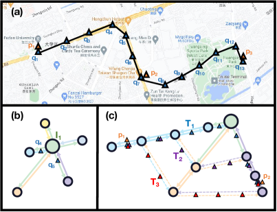
Figure 1: An example of trajectory recovery task and detailed illustration to demonstrate the significance of road network structure.

To facilitate the understanding of the above two limitations, we plot an example in Fig. 1(a). The three orange-colored points labelled as $p_{i}$ ($i\in[1,3]$) form an input trajectory of low sample rate. As observed, the distance between each two consecutive points is relatively long (as there are many missing GPS points between them). The task of trajectory recovery is to recover the missing points and map all the GPS points (including the input points and recovered points) to the road network to generate a high-sample trajectory, e.g., the 13 blue-colored points labelled as $q_{j}$ ($j\in[1,13]$) together with the underlying road segments (represented by black color lines) shown in Fig. 1(a) form an output trajectory.

This task is not trivial. Both the road network structure and context information of the input trajectory are essential to guarantee the high accuracy of the recovered trajectories. Their significance lies in four aspects. i) When two newly generated consecutive points are located at two different road segments, we have to rely on the road network to recover the trajectory. As illustrated in Fig. 1(b), new points $q_{4}$ and $q_{5}$ are near a major intersection $I_{1}$ that has complex topology. It’s impossible to recover the underlying road segments if the road network structure is not considered. Note in Fig. 1(b) and (c), circles represent intersections and lines with arrows stand for directional road segments from one intersection to another. ii) Raw GPS points by nature have errors (e.g., most GPS-enabled smartphones are accurate to within a 4.9 m radius under open sky). As shown in Fig. 1(a), raw GPS points $p_{1}$, $p_{2}$ and $p_{3}$ are not located at any road segments. Consequently, underlying road network provides an effective means to correct the errors as vehicles must move along the road network. iii) Raw points in the input trajectory might be far away from each other, and underlying road network reveals how vehicles can move from a point to another, e.g., we cannot simply use a straight line to connect $p_{1}$ to $p_{2}$ in Fig. 1(a). iv) Two consecutive GPS points in the input trajectory may be located at two different road segments while there are multiple candidate routes available to connect them. For example, we plot three candidate routes from $p_{1}$ to $p_{2}$ in Fig. 1(c), where triangles of the same color form one candidate route. The contextual information of the trajectory provides useful clues when filtering out impossible candidate route(s). For example, the position of $p_{3}$ suggests that the candidate route $T_{3}$ is unlikely to be the one as it requires detour to travel from $p_{2}$ to $p_{3}$. Those familiar with map matching might notice that some aspects discussed above are applicable to map matching too. Map matching could be considered as a sub-step of trajectory recovery, while trajectory recovery is more challenging as it not only maps GPS points to road segments but also recovers missing GPS points that truly capture a vehicle’s movement.

To address the limitations of existing trajectory recovery methods and meanwhile take advantage of end-to-end framework, we propose a novel transformer-based model, namely RNTrajRec, a Road Network enhanced Trajectory Recovery framework with spatial-temporal transformer. To capture the road network structure, RNTrajRec first develops a grid-partitioned road network representation module, namely GridGNN, to learn the hidden-state embedding for each road segment. To capture both the spatial-temporal features and the contextual information of trajectory, RNTrajRec then develops a novel transformer-based model, namely GPSFormer, which first represents each GPS point in a trajectory as a sub-graph road network that surrounds the GPS point through a Sub-Graph Generation module, and then introduces a novel spatial-temporal transformer model to learn rich spatial and temporal patterns of a GPS trajectory. It finally adopts a well-designed decoder proposed in [11] on top of the encoder model to recover the missing GPS points in the trajectory. Overall, our major contributions are summarized below.

• We propose a novel framework, namely RNTrajRec. To the best of our knowledge, RNTrajRec is the first attempt to combine road network representation with GPS trajectory representation for the task of trajectory recovery.

• To consider the road network structure around each GPS point in a given trajectory, we propose a novel spatial-temporal transformer network, namely GPSFormer, which consists of a transformer encoder layer for temporal modeling and a graph transformer model, namely graph refinement layer, for spatial modeling. Meanwhile, a Sub-Graph Generation module is developed to capture the spatial features for each GPS point.

• We propose a novel model for road network representation, namely GridGNN, which seamlessly combines grid-level representation with road network representation.

• We conduct extensive experiments on three real-life datasets to compare RNTrajRec with existing methods. Experimental results demonstrate that RNTrajRec significantly outperforms state-of-the-art solutions.

II Related Work

Spatial-Temporal Transformer. Transformers have achieved great success in many artificial intelligence fields, such as natural language processing [22, 23, 24] and computer vision [25, 26, 27]. Therefore, it has naturally attracted a lot of interest from academia and industry with many variants [28, 29, 30] being proposed. As a result, there is a growing interest in applying transformer architecture for graph representation[31, 32, 33]. However, most of these works solve graph modeling on fixed graph structure, which is not suitable for modeling dynamic graphs with temporal dependency.

Recently, several works have been proposed for dynamic graph modeling with transformer framework to solve pedestrian trajectory prediction[34], dynamic scene graph generation[35], 3D human pose estimation[36], activity recognition[37, 38] and etc. Specifically, Yu et al [34] propose a novel spatio-temporal transformer framework with intra-graph crowd interaction for trajectory prediction. However, the number of pedestrians (i.e. the number of nodes at each timestamp) is quite small and fixed. Cong et al [35] use the same transformer structure for both spatial and temporal modeling with a masked multi-head self-attention layer for temporal modeling. However, the time cost for each layer is $O\left(l^{2}\cdot v^{2}\right)$, with $l$ the length of the sequence and $v$ the averaged number of nodes in each graph structure. Zheng et al [36] use a patch embedding for spatial position embedding and propose a spatial attention network. However, the input and the output have different structures and hence the model is not stackable. Li et al [37] propose a spatial-temporal transformer framework tailored for group activity recognition. Zhang et al [38] propose a spatial-temporal transformer with a directional temporal transformer block to capture the movement patterns of human posture.

In this work, we regard a GPS point as a weighted sub-graph of the road network surrounding the GPS point. Therefore, the graph structures of points along a trajectory could be different from each other. We propose a spatial-temporal transformer network that has the following three advantages. i) Our model is more flexible as it has zero restriction on the number of nodes or edges for each graph. ii) The time cost for each layer is $O\left(l^{2}+l\cdot v\right)$, which is more efficient and scalable. Note that due to the sparseness of road network, a sub-graph of a road network with $v$ road segments only has $O\left(v\right)$ edges connecting these road segments. iii) The input and the output share the same structure, therefore, our model is stackable.

Road Network Representation Learning. Most of the existing works regard road network as a directed graph. Node2vec [39] and DeepWalk [40] are two novel models to model road segments as shallow embeddings. With the rapid development of graph neural network (GNN), many graph convolutional networks (e.g., GCN [41], GraphSage [42], GAT [43] and GIN [44]) are suitable for road network representation. Recently, several works have been proposed specifically for road network representation learning [45, 46, 47]. Among them, STDGNN [45] regards road network as a dual graph structure with a node-wise GCN modeling the features of intersections and an edge-wise GCN modeling the features of road segments, HRNR [46] constructs a three-level neural architecture to learn rich hierarchical features of road network, and Toast [47] proposes a traffic context aware skip-gram module for road network representation and a trajectory-enhanced transformer module for route representation.

In this work, we regard each road segment as a sequence of grids that the road segment passes through and use recurrent neural network to model grid sequence dependency and graph neural network to model graph structure. With this design, our road network representation can capture both nearby neighborhood features and graph topology features.

GPS Trajectory Representation Learning. Learning-based methods for representing GPS trajectory have been studied wildly these years. Among them, T2vec [6], NeuTraj [7], T3S [8], and Traj2SimVec [9] are representative models. T2vec proposes the first deep learning model for trajectory similarity learning with BiLSTM [48] modeling temporal dependency. NeuTraj integrates a spatial-memory network for trajectory encoding and uses distance-weighted rank loss for accurate and effective trajectory representation learning. T3S uses a self-attention based network for structural information representation and a LSTM [48] module for spatial information representation. Traj2SimVec proposes a novel sub-trajectory distance loss and a trajectory point matching loss for robust trajectory similarity computation. However, these works only consider GPS trajectory in Euclidean space but ignore the important road network topology. Recently, Han et al [10] propose a graph-based method along with a novel spatial network based metric similarity computation. However, it mainly focuses on representing point-of-interests (POIs) in road networks. Since POIs are discrete GPS points on road network and GPS points in a trajectory are continuous, it cannot be directly used for GPS trajectory representation learning. To the best of our knowledge, our work is the first attempt to solve GPS trajectory representation learning in spatial networks.

Trajectory Recovery. Recovering low sample trajectory is important for reducing uncertainty [19, 49, 50, 11]. Specifically, DHTR [19] proposes a two-stage solution that first recovers high-sample trajectory followed by a map matching algorithm (i.e. HMM [14]) to recover the real GPS locations. AttnMove [49] designs multiple intra- and inter- trajectory attention mechanisms to capture user-specific long-term and short-term patterns. Bi-STDDP [50] integrates bi-directional spatio-temporal dependence and users’ dynamic preferences to capture complex user-specific patterns. However, both AttnMove and Bi-STDDP use user-specific history trajectories and are designed for recovering missing POI check-in data, which is very different from our setting. MTrajRec [11] proposes an end-to-end solution with a map-constraint decoder model, which significantly outperforms two-stage methods. However, it ignores the important road network structure, leaving rooms for further improving the accuracy. In this paper, we propose a novel GPSFormer module to learn rich spatial and temporal features of trajectories from the road network.

III Preliminary

TABLE I: The Summary of notations

Notation	Definition
$G$	The topology structure of the road network.
$\hat{G}_{\tau}$	The subgraphs structure for the given trajectory $\tau$.
$\hat{G}_{\tau,i}$	The subgraph structure of the $i^{th}$ sample point in the given trajectory $\tau$.
$\Sigma^{grid}$	The grid embedding table.
$\Sigma^{road}$	The road segment embedding table.
$e_{i},\bar{e},\tilde{e},\hat{e}$	A certain road segment in the road network.
$X^{road}$	The representation of the road network.
$\vec{Z}_{\tau}^{(l)}$	The representation for the subgraphs of the given trajectory $\tau$ after $l$ layers of GPSFormer.
$\vec{Z}_{\tau,i}^{(l)}$	The representation for the subgraph of the $i^{th}$ sample in the given trajectory $\tau$ after $l$ layers of GPSFormer.
$\vec{H}_{\tau}^{(l)}$	The input features for the given trajectory $\tau$ to the transformer encoder layer at the $l^{th}$ layer of GPSFormer.
$H_{\tau}^{traj}$	The final representation for every sample point in the given trajectory $\tau$.
$h_{\tau}^{traj}$	The final trajectory-level representation for the given trajectory $\tau$.
$c$	The constraint mask vector defined in the decoder model.
$\mathcal{L}_{id},\mathcal{L}_{rate},\mathcal{L}_{enc}$	The loss functions employed in RNTrajRec.

In this section, we formally introduce the key concepts related to this work and define the task of trajectory recovery. The notations used in this paper are briefly summarized in Table I and fully explained throughout the paper.

Definition 1: (Road Network.) A Road Network is modeled as a directed graph $G=\left(V,E\right)$, where $V$ represents the set of road segments and $E\subseteq V\times V$ captures the connectivity of these road segments, i.e., an edge $\langle e_{i},e_{j}\rangle\in E$ if and only if there exists a direct connection from road segment $e_{i}$ to road segment $e_{j}$.

Definition 2: (Trajectory.) A Trajectory $\tau/\rho$ is defined as a sequence of $l$ tuples, i.e. $\tau/\rho=\langle\left(p_{1},t_{1}\right)$, $\left(p_{2},t_{2}\right)$, $\cdots$, $\left(p_{l},t_{l}\right)\rangle$, where $l$ refers to the length of the trajectory, $p_{i}$ refers to the $i^{th}$ sample point in $\tau$/$\rho$, and $t_{i}$ is the sample time of $p_{i}$ in $\tau$/$\rho$. Note, the time interval between two adjacent sample points in a trajectory (i.e., $t_{i+1}-t_{i}$) defines the sample interval $\epsilon$ of this trajectory.

GPS devices have measurement errors. Throughout the paper, we use terms Raw GPS Trajectory and Map-matched GPS Trajectory to refer to a GPS trajectory (denoted as $\tau$) directly obtained from certain GPS device and that (denoted as $\rho$) after running a map matching algorithm (e.g. HMM [14]) respectively. Note, $p_{i}$ in a raw GPS trajectory $\tau$ records its exact location using latitude and longitude, while $p_{j}$ in a map-matched GPS trajectory $\rho$ captures its location based on the road segment $e_{j}$ that $p_{j}$ is located at and moving ratio $r_{j}\in[0,1)$ that captures the moving distance of $p_{j}$ over the total length of $e_{j}$ (e.g., if $r_{j}=0.5$, the point $p_{j}$ is located at the middle point of road segment $e_{j}$). In addition, a raw GPS trajectory $\tau$ typically does not have a fixed sample interval, and we use the average time interval $\epsilon_{\tau}$ instead. A low-sample trajectory has a long sample interval.

Definition 3: (Map-matched $\epsilon_{\rho}$-Sample Interval Trajectory.) A Map-matched $\epsilon_{\rho}$-Sample Interval Trajectory $\rho$ is a Map-matched GPS Trajectory with a fixed sample interval $\epsilon_{\rho}$, i.e., $\rho=\langle\left(q_{1},t_{1}\right),\left(q_{2},t_{1}+\epsilon_{\rho}\right),\cdots,\left(q_{l_{\rho}},t_{1}+(l_{\rho}-1)\epsilon_{\rho}\right)\rangle$.

Definition 4: (Trajectory Recovery.) Given a low-sample Raw GPS Trajectory $\tau$ with measurement errors (e.g., orange GPS points in Fig. 1(a)), the task of Trajectory Recovery aims to recover the real Map-matched $\epsilon_{\rho}$-Sample Interval Trajectory $\rho$ (e.g., blue GPS points in Fig. 1(a)). Specifically, for each low-sample trajectory, it infers the missing GPS points and maps each GPS point (including the GPS points in the input trajectory $\tau$) onto the road network to obtain the real GPS locations of the moving trajectory. Note that the sample interval $\epsilon_{\rho}$ of the recovered trajectory $\rho$ must be much smaller than that of the given Raw GPS Trajectory $\epsilon_{\tau}$.

IV Methodology

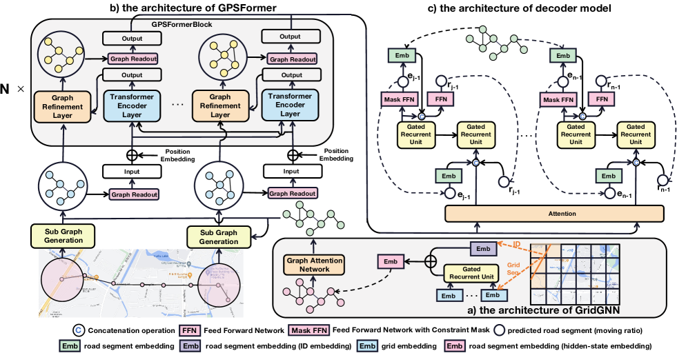
Figure 2: The framework of RNTrajRec. (a) The architecture of GridGNN. For each road segment, a grid GRU cell is used to aggregate the grid sequence followed by a stack of $M$ GAT modules to capture the spatial information. (b) The architecture of GPSFormer. Given a GPS trajectory, GPSFormer first extracts the road network features around each GPS point through the Sub-Graph Generation module. The features along with the sub-graphs are passed through several spatial-temporal transformer layers to learn the spatial and temporal features. (c) The architecture of decoder model. Given the output from the encoder model, an attention module is adopted to compute the similarity between the hidden-state vector of GRU cell and the outputs of encoder model and generate the input hidden-state vectors $a^{(j)}$ for timestamp $j$. A multi-task learning module is proposed that first predicts the target road segment $e_{j}$, followed by a regression task for predicting moving ratio on the predicted road segment, i.e. $r_{j}$. The entire model is trained end-to-end with Adam optimizer.

This section introduces our proposed RNTrajRec, with the overall framework presented in Fig. 2.

IV-A Model Overview

The first component of RNTrajRec is GridGNN, a grid-partitioned road network representation module that learns spatial features for each road segment, as shown in Fig. 2(a). Given a road network $G=\left(V,E\right)$, GridGNN learns rich road network features $X^{road}\in\mathbb{R}^{|V|\times d}$, where $d$ is the hidden size of the model.

The second component of RNTrajRec is GPSFormer, a spatial-temporal transformer based GPS trajectory encoder that encodes raw GPS points $\langle p_{1},p_{2},\cdots,p_{l_{\tau}}\rangle$ in a trajectory $\tau$ into hidden vectors, as shown in Fig. 2(b). To obtain the input of GPSFormer, we first extract the road network features around each GPS point $p_{i}$ through the Sub-Graph Generation module. After the generation process, each GPS point $p_{i}\in\tau$ is represented as a weighted directed sub-graph $\hat{G}_{\tau,i}=\left(V_{\tau,i},E_{\tau,i},W_{\tau,i}\right)$, where $V_{\tau,i}$ captures the road segments selected by the module that surround the GPS point $p_{i}\in\tau$, $E_{\tau,i}$ is the set of edges in the selected sub-graph of the road network, and $W_{\tau,i}$ refers to the set of weights between $p_{i}$ and each selected road segment in the sub-graph. Note that we use $\hat{G}$ instead of $G$ to represent a sub-graph. Each generated sub-graph gathers road network features from $X^{road}$ to form its initial representation, i.e. $\vec{Z}_{\tau,i}^{(0)}\in\mathbb{R}^{|V_{\tau,i}|\times d}$. We further perform weighted mean pooling on graph to get the input representation of the trajectory $\tau$, i.e. $\hat{H}_{\tau}^{(0)}\in\mathbb{R}^{l_{\tau}\times d}$. We then forward a mini-batch of $b$ trajectory features along with the sub-graph structure into $N$ stacked GPSFormerBlock layers, which is a combination of transformer encoder layer for temporal modeling and graph refinement layer, namely GRL, for spatial modeling.

The last component of RNTrajRec is a decoder model, proposed in [11] specifically designed for trajectory recovery task. Given the outputs of a mini-batch of $b$ trajectories from the encoder model, i.e. $\vec{H}^{(N)}\in\mathbb{R}^{b\times l_{\tau}\times d}$, the decoder model first uses an attention module to calculate the similarity between the hidden-state vectors of the Gated Recurrent Unit (GRU)[21] cell (i.e., the query vectors) and the outputs from the encoder model (i.e., the key vectors) to obtain the input hidden vector $a^{(j)}$ at the $j^{th}$ timestamp. Furthermore, a multi-task learning module is proposed specifically for trajectory recovery task that first predicts the target road segment $e_{j}$ and then predicts the corresponding moving ratio $r_{j}$ via a regression task, which will be detailed in Section V.

IV-B Road Network Representation: GridGNN

As stated in Section I, the road network structure is essential for the task of trajectory recovery. GridGNN is proposed to well capture the spatial features of road network. It partitions the road network into $m\times n$ equal-sized grid cells. Accordingly, each road segment can be represented as a sequence of grids that the road segment passes through. Formally speaking, we build a grid embedding table $\Sigma^{grid}\in\mathbb{R}^{m\times n\times d}$ for each grid cell. Similarly, given the road network $G=\left(V,E\right)$, we create a road segment embedding table $\Sigma^{road}\in\mathbb{R}^{|V|\times d}$, where $|V|$ is the total number of road segments in the road network.

For each road segment $e_{i}\in V$, let $S_{i}=\langle\tilde{g}_{i}^{1},\tilde{g}_{i}^{2},...,\tilde{g}_{i}^{\phi_{i}}\rangle$ be a sequence of $\phi_{i}$ grids passed through by $e_{i}$. Since the grid sequence of each road segment has sequential dependencies, we use GRU cell to model the grid-level representation. That is, for each road segment $e_{i}$ and its corresponding grid sequence $S_{i}$, the grid-level hidden-state vector is given by:

$$\begin{array}[]{rl}g_{i}^{(j)}=&\operatorname{lookup}(\tilde{g}_{i}^{j}.x,\tilde{g}_{i}^{j}.y)\\ z_{i}^{(j)}=&\sigma\left(\mathbf{W}_{z}\cdot\left[s_{i}^{(j-1)},g_{i}^{(j)}\right]+\mathbf{b}_{z}\right)\\ r_{i}^{(j)}=&\sigma\left(\mathbf{W}_{r}\cdot\left[s_{i}^{(j-1)},g_{i}^{(j)}\right]+\mathbf{b}_{r}\right)\\ c_{i}^{(j)}=&tanh\left(\mathbf{W}_{c}\cdot\left[r_{i}^{(j)}*s_{i}^{(j-1)},g_{i}^{(j)}\right]+\mathbf{b}_{c}\right)\\ s_{i}^{(j)}=&\left(1-z_{i}^{(j)}\right)*s_{i}^{(j-1)}+z_{i}^{(j)}*c_{i}^{(j)}\\ \end{array}$$ (1)

Here, $j\in\{1,2,\cdots,\phi_{i}\}$, $\operatorname{lookup}\left(i,j\right)$ retrieves the grid embedding of position $\left(i,j\right)$ from the grid embedding table $\Sigma^{grid}$, $\mathbf{W}_{x}$ represents the weight for the gate($x$) neurons, $\mathbf{b}_{x}$ represents the bias for gate($x$), and $\sigma\left(\cdot\right)$ represents the gated function, which is implemented as sigmoid function. The initial embedding for each road segment $r_{i}^{(0)}$ is:

$$r_{i}^{(0)}=\operatorname{ReLU}(s_{i}^{(\phi_{i})}+\sigma_{i}^{road})$$ (2)

Here, $\sigma_{i}^{road}\in\mathbb{R}^{d}$ is the road segment embedding of the $i^{th}$ road segment from $\Sigma^{road}$.

The obtained hidden-state vector $r_{i}^{(0)}$ considers each road segment independently, which does not capture the topology of the road network structure. In order to enhance the representation of road network, we integrate GNN. Specifically, we stack $M$ layers of Graph Attention Network (GAT) module, which uses multi-head attention to efficiently learn the complex graph structure, to obtain final hidden-state vectors $\hat{X}^{road}\in\mathbb{R}^{|V|\times d}$:

$$a_{ij,k}^{(l)}= \frac{\exp\left(\operatorname{LeakyReLU}\left(\overrightarrow{\mathrm{a^{k}}}\left[\mathbf{\widehat{W}}^{k}r_{i}^{(l-1)}\|\mathbf{\widehat{W}}^{k}r_{j}^{(l-1)}\right]\right)\right)}{\sum_{n\in N_{i}}\exp\left(\operatorname{LeakyReLU}\left(\overrightarrow{\mathrm{a^{k}}}\left[\mathbf{\widehat{W}}^{k}r_{i}^{(l-1)}\|\mathbf{\widehat{W}}^{k}r_{n}^{(l-1)}\right]\right)\right)}$$ (3)

$$r_{i}^{(l)}= \|_{k=1}^{h}\operatorname{LeakyReLU}\left(\sum\nolimits_{j\in\mathcal{N}_{i}}a_{ij,k}^{(l)}\mathbf{W}^{k}r_{j}^{(l-1)}\right)\quad\quad\$$ (4)

Here, $l\in\{1,2,\cdots,M\}$. For the $k^{th}$ attention head, $a_{ij,k}^{(l)}$ represents the attention score between road segments $e_{i}$ and $e_{j}$ at the $l^{th}$ layer, $\overrightarrow{\mathrm{a}^{k}}$ are learnable weights to obtain attention scores, $\mathbf{W}^{k}$ and $\mathbf{\widehat{W}}^{k}$ is a learnable weight for feature transformation. $\left[\cdot\|\cdot\right]$ represents the concatenation operation, and $N_{i}$ represents the neighborhood of road segment $e_{i}$ in the road network.

The final road network representation is given by the concatenation of $\hat{X}^{road}=\{r_{i}^{(M)}\}$ for each $e_{i}\in V$ and the static features $f_{s}^{road}\in\mathbb{R}^{|V|\times f_{r}}$ (i.e. length of the road segment, number of in/out-going edges, etc), followed by linear transformation to obtain $d$ dimension vectors $X^{road}$.

IV-C Sub-Graph Generation

Given the representation $X^{road}\in\mathbb{R}^{|V|\times d}$ of the road network, a straight-forward way to obtain the representation of a GPS point is to average over the embeddings of the road segments around the GPS point. However, this approach suffers from the following two problems. a) The influence of the nearby road segments on the given GPS point varies significantly. b) For each GPS point in a trajectory, its surrounding sub-graph structure is important for understanding the movement of the trajectory. Therefore, it is necessary to take the graph structure into consideration.

For a given GPS point $p$, we first locate the road segments within at most $\delta$ meters away from $p$, via R-tree[51] or any other spatial data structure. Note, $\delta$ is a hyper-parameter to control the receptive field of the GPS point. Assume in total $\omega_{p}$ road segments are returned, denoted as $\{e_{p}^{1},e_{p}^{2},\cdots,e_{p}^{\omega_{p}}\}$. We further follow the road network $G=(V,E)$ to connect these $\omega_{p}$ road segments into a sub-graph $\tilde{G}^{p}=\left(V^{p},E^{p}\right)$, where $V^{p}=\{e_{p}^{1},e_{p}^{2},\cdots,e_{p}^{\omega_{p}}\}$ and $E^{p}=(V^{p}\times V^{p})\cap E$.

Following [11], we use the exponential function to model the influence of road segment $e$ on the given GPS point $p$, as defined in Eq. (5). Here, $\operatorname{dist}(e,p)$ represents the distance between the GPS point $p$ and the road segment $e$, i.e. spherical distance between the GPS point $p$ and its projection to the road segment $e$, and $\gamma$ is a hyper-parameter with respect to the road network. To this end, we obtain the weighted sub-graph of a given GPS point, i.e. $\tilde{G}^{p}=\left(V^{p},E^{p},W^{p}\right)$, where $W^{p}$ can be derived by Eq. (5).

$$\omega(e,p) = \exp\left({-\operatorname{dist}^{2}(e,p)}/{\gamma^{2}}\right)$$ (5)

$$g^{p} = {\sum\nolimits_{\hat{e}\in V^{p}}W_{\hat{e}}^{p}*x_{\hat{e}}^{road}}/{\sum\nolimits_{\hat{e}\in V^{p}}W_{\hat{e}}^{p}}$$ (6)

We use mean pooling on graph to get the representation of a given GPS point $p$, as defined in Eq. (6). Here, $x_{\hat{e}}^{road}$ represents the road segment representation of road segment $\hat{e}$ obtained from $X^{road}$ and $W_{\hat{e}}^{p}$ represents the influence of road segment $\hat{e}$ on the GPS point $p$, i.e. $W_{\hat{e}}^{p}=\omega(\hat{e},p)$.

Given a trajectory $\tau=\langle\left(p_{1},t_{1}\right),\left(p_{2},t_{2}\right),\cdots,\left(p_{l_{\tau}},t_{l_{\tau}}\right)\rangle$, its hidden-state vector $H^{traj}_{\tau}\in\mathbb{R}^{{l_{\tau}}\times\left(d+3\right)}$ concatenates the road network empowered GPS representation $g_{\tau}=\langle g^{p_{1}}$,$g^{p_{2}}$, $\cdots$, $g^{p_{l_{\tau}}}\rangle$ $\in\mathbb{R}^{l_{\tau}\times d}$, timestamp sequence $\hat{t}_{\tau}=$ $\langle t_{1}$, $t_{2}$, $\cdots$, $t_{l_{\tau}}\rangle$ $\in\mathbb{R}^{l_{\tau}\times 1}$ and grid index $\hat{g}_{\tau}=$ $\langle(x_{1},y_{1})$, $(x_{2},y_{2})$, $\cdots$, $(x_{l_{\tau}},y_{l_{\tau}})\rangle\in\mathbb{R}^{l_{\tau}\times 2}$, where $(x_{i},y_{i})$ represents the index of the grid that the GPS point $p_{i}$ falls inside. Finally, we map $H^{traj}_{\tau}$ into $d$ dimension vectors $\hat{H}_{\tau}^{(0)}$ through linear transformation.

For the sub-graph input of the given trajectory $\tau$, $\hat{G}_{\tau}=$ $\langle\hat{G}_{\tau,1}$, $\hat{G}_{\tau,2}$, $\cdots,\hat{G}_{\tau,l_{\tau}}\rangle$, where $\hat{G}_{\tau,i}=\tilde{G}^{p_{i}}$ represents the generated weighted sub-graph for GPS point $p_{i}$. The initial graph-level sequence $\vec{Z}_{\tau}^{(0)}=\langle\vec{Z}_{\tau,1}^{(0)},\vec{Z}_{\tau,2}^{(0)},\cdots,\vec{Z}_{\tau,l_{\tau}}^{(0)}\rangle$, where $\vec{Z}_{\tau,i}^{(0)}=\{x_{\hat{e}}^{road}\}$ for every road segment $\hat{e}\in V_{\tau,i}$.

IV-D Graph Refinement Layer (GRL)

As mentioned in Section IV-C, graph structure is significant for representing GPS points in spatial network. To this end, we propose a graph refinement layer (GRL) that is capable of capturing rich spatial features.

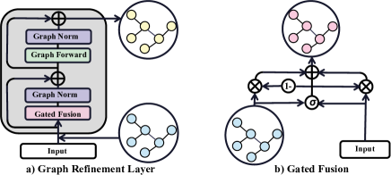
Figure 3: The framework Graph Refinement Layer (GRL) module.

Fig. 3 shows the architecture of the proposed graph refinement layer. Though it is inspired by the encoder of transformer model, there are five major differences between transformer encoder and the newly proposed GRL. a) Transformer encoder captures the temporal features across the sequence, while GRL captures the spatial features and uses the output of transformer encoder to update the local features. b) Transformer encoder only takes hidden vectors as input, while GRL takes both the hidden vectors and graph structures as input. c) Motivated by [33] which demonstrates that batch normalization[52] is more suitable for graph transformer, GRL replaces layer normalization[22] with a newly proposed graph normalization, which can be viewed as an extension of batch normalization for graph representation with temporal dependency, to normalize the hidden vectors. d) GRL replaces multi-head attention in transformer encoder with gated fusion[4] to adaptively fuse the input hidden vectors and the node features in the graph structure. e) GRL further replaces the feed forward in transformer encoder with graph forward to capture the rich spatial features around GPS points.

Assume the output hidden vectors at layer $l$ are $\vec{H}_{\tau}^{(l)}\in\mathbb{R}^{l_{\tau}\times d}$, and the corresponding output graph hidden vectors are $\vec{Z}_{\tau}^{(l)}$, where each sub-graph features $\vec{Z}_{\tau,i}^{(l)}\in\mathbb{R}^{|V_{\tau,i}|\times d}$. Following [22], we employ a residual connection for both gated fusion sub-layer and graph forward sub-layer, followed by graph normalization. That is, the output of each sub-layer is given by $\operatorname{GraphNorm}\left(x+\operatorname{SubLayer}\left(x\right)\right)$, where $\operatorname{SubLayer}$ represents a function that can be either $\operatorname{GatedFusion}$ or $\operatorname{GraphForward}$. $\operatorname{GraphForward}$ is implemented as a stack of $P$ standard GAT modules defined in Eq. (3) and Eq. (4), while $\operatorname{GatedFusion}$ and $\operatorname{GraphNorm}$ are detailed below.

IV-D1 Gated Fusion

The hidden-state vectors from the output of transformer encoder layer, i.e. $\vec{Tr}_{\tau}^{(l)}$, capture rich temporal features of the given trajectory, while the graph structure, i.e. $\hat{G}_{\tau}$, captures rich spatial information of each GPS point in the trajectory. Therefore, it is necessary to design a fusion mechanism to adaptively fuse the spatial and temporal features. Inspired by [4], we propose to use gated fusion to combine the hidden vectors at the $i^{th}$ timestamp, i.e. $tr_{\tau,i}^{(l)}\in\mathbb{R}^{d}$ with the corresponding graph features $\vec{Z}_{\tau,i}^{(l-1)}\in\mathbb{R}^{|V_{\tau,i}|\times d}$:

$$\tilde{Z}_{\tau,i}^{(l)} = z_{\tau,i}^{(l)}\odot\hat{tr}_{\tau,i}^{(l)}+\left(1-z_{\tau,i}^{(l)}\right)\odot\vec{Z}_{\tau,i}^{(l-1)}$$

$$z_{\tau,i}^{(l)} = \sigma\left(\hat{tr}_{\tau,i}^{(l)}\mathbf{W}_{z,1}+\vec{Z}_{\tau,i}^{(l-1)}\mathbf{W}_{z,2}+\mathbf{b}_{z}\right)$$ (7)

Here, $\hat{tr}_{\tau,i}^{(l)}\in\mathbb{R}^{|V_{\tau,i}|\times d}$ repeats $tr_{\tau,i}^{(l)}$ for $|V_{\tau,i}|$ times to ensure that $\hat{tr}_{\tau,i}^{(l)}$ and $\vec{Z}_{\tau,i}^{(l-1)}$ share the same size, $\mathbf{W}_{z,1},\mathbf{W}_{z,2}$ and $\mathbf{b}_{z}$ represent the learnable weights in the module and $\sigma\left(\cdot\right)$ is the gated activation function, which is implemented as a sigmoid activation function.

IV-D2 Graph Norm

Inspired by [33], we replace layer normalization with graph normalization to normalize graph features within a mini-batch. A mini-batch of input graph structures can be represented as $\{\hat{G}_{\tau_{1}},\hat{G}_{\tau_{2}},\cdots,\hat{G}_{\tau_{b}}\}$ with hidden-state graph features $\{\tilde{Z}_{\tau_{1}}^{(l)},\tilde{Z}_{\tau_{2}}^{(l)},\cdots,\tilde{Z}_{\tau_{b}}^{(l)}\}$, which can be the output of either $\operatorname{GatedFusion}$ sub-layer or $\operatorname{GraphForward}$ sub-layer, where $\tilde{Z}_{\tau}^{(l)}=\{\tilde{Z}_{\tau,i}^{(l)}\}$ for each $i\in\{1,2,\cdots,l_{\tau}\}$ and $b$ represents the batch size.

We first perform mean pooling to obtain graph feature for each sub-graph via Eq. (8). Here, $M^{(l)}=\{m_{\tau_{i},j}^{(l)}\}$ for each $i\in\{1,2,\cdots,b\}$ and $j\in\{1,2,\cdots,l_{\tau}\}$. Note that we assume trajectories $\tau$ in a mini-batch share the same length $l_{\tau}$.

$$m_{\tau_{i},j}^{(l)}=\frac{1}{|V_{\tau_{i},j}|}\sum\nolimits_{k=1}^{|V_{\tau_{i},j}|}\tilde{Z}_{\tau_{i},j,k}^{(l)}$$ (8)

We then perform batch normalization on $M^{(l)}\in\mathbb{R}^{b\times l_{\tau}\times d}$ with the features $\{\tilde{Z}_{\tau_{1}}^{(l)},\tilde{Z}_{\tau_{2}}^{(l)},\cdots,\tilde{Z}_{\tau_{b}}^{(l)}\}$ to get the output $\vec{Z}_{\tau}^{(l)}$:

$$\begin{array}[]{rl}\mu_{\mathcal{B}}=&\frac{1}{b\times l_{\tau}}\sum_{i=1}^{b}\sum_{j=1}^{l_{\tau}}M_{\tau_{i},j}^{(l)}\vspace{2ex}\\ \sigma_{\mathcal{B}}=&\frac{1}{\sum_{i=1}^{b}\sum_{j=1}^{l_{\tau}}|V_{\tau_{i},j}|}\sum_{i=1}^{b}\sum_{j=1}^{l_{\tau}}\sum_{k=1}^{|V_{\tau_{i},j}|}\left(\tilde{Z}_{\tau_{i},j,k}-\mu_{\mathcal{B}}\right)^{2}\vspace{2ex}\\ \widetilde{Z}_{\tau}^{(l)}=&\frac{\tilde{Z}_{\tau}^{(l)}-\mu_{\mathcal{B}}}{\sqrt{\sigma_{\mathcal{B}}+\epsilon}}\vspace{2ex}\\ \vec{Z}_{\tau}^{(l)}=&\gamma_{\mathcal{B}}\widetilde{Z}_{\tau}^{(l)}+\beta_{\mathcal{B}}\end{array}$$ (9)

Here, $\gamma_{\mathcal{B}}$ and $\beta_{\mathcal{B}}$ are learnable parameters for scalar transformation and shift transformation in batch normalization respectively, and $\vec{Z}_{\tau}^{(l)}$ is the output of graph normalization.

IV-E Transformer Encoder Layer

Transformer encoder layer contains a multi-head attention sub-layer and a feed forward sub-layer with a residual connection for each of the two sub-layers, followed by layer normalization. That is, the output of each sub-layer is given by $\operatorname{LayerNorm}\left(x+\operatorname{SubLayer}\left(x\right)\right)$, where $\operatorname{SubLayer}$ represents a function that can be either $\operatorname{MultiHead}$ or $\operatorname{FFN}$.

IV-E1 Multi-Head Attention

Given a sequence input $X\in\mathbb{R}^{L\times d}$ with $L$ the length of the sequence, multi-head attention is given by:

$$\operatorname{MultiHead\left(Q,K,V\right)} = Concat\left(head_{1},\cdots,head_{h}\right)W^{O}$$

$$head_{i} = \operatorname{Attention}\left(QW_{i}^{Q},KW_{i}^{K},VW_{i}^{V}\right)$$

$$\operatorname{Attention\left(Q,K,V\right)} = \text{softmax}\left(\frac{QK^{T}}{\sqrt{d}}\right)V$$ (10)

Here, $Q$, $K$ and $V$ refer to the query, the keys and the values for the input $X$ respectively, $W_{i}^{Q}$, $W_{i}^{K}$ and $W_{i}^{V}$ are the learnable parameters of the $i^{th}$ attention head for the query, the keys and the values respectively, $W^{O}$ is a learnable parameter for the output, and $h$ captures the number of attention heads.

IV-E2 Feed Forward

Feed-forward network contains a fully connected network with ReLU activation function:

$$FFN\left(x\right)=\operatorname{ReLU}\left(xW_{1}+b_{1}\right)W_{2}+b_{2}$$ (11)

Here, $W_{1}$ and $W_{2}$ are two learnable weights, and $b_{1}$ and $b_{2}$ are the bias for the layer.

IV-F GPSFormer

GPSFormer first extracts spatial features for each GPS point in the trajectory through the Sub-Graph Generation module introduced in Session IV-C, and then applies $N$ layers of GPSFormerBlock to capture rich trajectory patterns.

Given a mini-batch of $b$ trajectories $\{\tau_{1},\tau_{2},\cdots,\tau_{b}\}$. We first obtain the initial hidden-state vectors are $\widehat{H}_{\tau}^{(0)}=$ $\{\hat{H}_{\tau_{1}}^{(0)}$, $\hat{H}_{\tau_{2}}^{(0)}$, $\cdots$, $\hat{H}_{\tau_{b}}^{(0)}\}$ $\in\mathbb{R}^{b\times l_{\tau}\times d}$, accompanied by the initial graph structure $\widehat{G}_{\tau}=$ $\{\hat{G}_{\tau_{1}}$, $\hat{G}_{\tau_{2}}$, $\cdots,\hat{G}_{\tau_{b}}\}$ and initial graph features $\vec{Z}_{\tau}^{(0)}=$ $\{\vec{Z}_{\tau_{1}}^{(0)}$, $\vec{Z}_{\tau_{2}}^{(0)}$, $\cdots,\vec{Z}_{\tau_{b}}^{(0)}\}$ though the Sub-Graph Generation module.

After that, we first add position embedding[22] to $\widehat{H}_{\tau}^{(0)}$ and obtain the input to the transformer encoder:

$$\vec{H}_{\tau}^{(0)}=\widehat{H}_{\tau}^{(0)}+PE\left(\widehat{H}_{\tau}^{(0)}\right)$$ (12)

Next, we input the hidden-state vectors and graph structures to a stacked of $N$ GPSFormer cells:

$$\begin{array}[]{rl}\vec{Tr}_{\tau}^{(l)}=&\operatorname{TransformerEncoder}\left(\vec{H}_{\tau}^{(l-1)}\right)\\ \vec{Z}_{\tau}^{(l)}=&\operatorname{GraphRefinement}\left(\vec{Tr}_{\tau}^{(l)},\vec{Z}_{\tau}^{(l-1)},\widehat{G}_{\tau}\right)\\ \vec{H}_{\tau}^{(l)}=&\operatorname{GraphReadout}\left(\vec{Z}_{\tau}^{(l)},\widehat{G}_{\tau}\right)\end{array}$$ (13)

Here, $\operatorname{TransformerEncoder}$ and $\operatorname{GraphRefinement}$ stand for the transformer encoder layer and the graph refinement layer introduced in Section IV-E and Section IV-D respectively, and $\operatorname{GraphReadout}$ represents graph mean pooling operation similar to Eq. (8). The final representation for a mini-batch trajectories is $H_{\tau}^{traj}=\vec{H}_{\tau}^{(N)}\in\mathbb{R}^{b\times l_{\tau}\times d}$. Besides, we concatenate the mean pooling of $H_{\tau}^{traj}$ with the environmental contexts $f^{e}_{\tau}\in\mathbb{R}^{b\times f_{t}}$ (e.g. hour of the day, holiday or not, etc), followed by linear transformation to obtain trajectory-level hidden-state vector $\hat{h}_{\tau}^{traj}\in\mathbb{R}^{b\times d}$.

IV-G Decoder Model

Let $H_{\tau}^{traj}$ be the outputs of the encoder model. For simplicity, we denote the representation of a single trajectory as $h^{traj}=\{h_{1},h_{2},\cdots,h_{l_{\tau}}\}$. The decoder model uses a GRU model to predict the road segment and moving ratio for each timestamp in the target trajectory. Assume the hidden-state vector in the GRU model at timestamp $t$ is given by $h_{gru}^{(t)}$ with $h_{gru}^{(0)}=\hat{h}_{\tau}^{traj}$. An attention mechanism is adopted to obtain the input of GRU cell, i.e. $a^{(t)}$:

$$a^{(t)}=\sum\nolimits_{i=1}^{l_{\tau}}\alpha_{i}^{(t)}h_{i}$$

$$\begin{array}[]{rl}\alpha_{i}^{(t)}&=\exp\left(\mu_{i}^{(t)}\right)/\sum_{k=1}^{l_{\tau}}\exp\left(\mu_{k}^{(t)}\right)\vspace{2ex}\\ \mu_{i}^{(t)}&=\mathbf{v}^{T}\cdot\operatorname{tanh}\left(\mathbf{W}_{g}h_{gru}^{(t-1)}+\mathbf{W}_{h}h_{i}\right)\end{array}$$ (14)

Here, $\mathbf{v}\in\mathbb{R}^{d\times 1}$ represents the transformation weight, and $\mathbf{W}_{g}$ and $\mathbf{W}_{h}$ are learnable weights in the attention module.

To this end, the hidden-state vectors of the GRU cell are updated by:

$$h_{gru}^{(j)}=\operatorname{GRU}\left(\left[x^{(j-1)}\|r^{(j-1)}\|a^{(j)}\right]\right)$$ (15)

Here, $j\in\left[1,2,\cdots,l_{\rho}\right]$, $x^{(j-1)}$ and $r^{(j-1)}$ represent the road segment embedding of the predicted road segment and its corresponding moving ratio at the $({j-1})^{th}$ timestamp, and $\operatorname{GRU}$ represents the GRU cell defined in Eq. (1). Finally, $h_{gru}^{(j)}$ is forwarded to a multi-task block to recover the missing trajectory.

V Multi-Task Learning for Trajectory Recovery

Given a mini-batch of $b$ trajectories, we first use the GPSFormer to obtain the trajectory representation for each sample, i.e., $H_{\tau}^{traj}\in\mathbb{R}^{b\times l_{\tau}\times d}$, and then forward the hidden-state vectors to the decoder model to obtain the hidden-state vectors of the GRU cell, i.e., $h_{gru}^{(j)}$. For the task of predicting road segment ID, following [11], we adopt the cross entropy as the loss function:

$$\mathcal{L}_{id}=-\sum\nolimits_{i=1}^{b}\frac{1}{{l_{\rho}}}\sum\nolimits_{j=1}^{{l_{\rho}}}\log\left(P_{\theta_{enc},\theta_{dec}}\left(\tilde{e}_{i}^{(j)}|h_{gru}^{(j)},c_{j}\right)\right)$$

$$P_{\theta_{enc},\theta_{dec}}\left(\tilde{e}_{i}^{(j)}|h_{gru}^{(j)},c_{j}\right)=\frac{\exp\left(h_{gru}^{(j)}\cdot{\mathbf{w}_{i}^{id}}\right)\odot c_{j,\tilde{e}_{i}^{(j)}}}{\sum_{v\in V}\exp\left(h_{gru}^{(j)}\cdot{\mathbf{w}_{v}^{id}}\right)\odot c_{j,v}}$$ (16)

Here, $\mathbf{w}^{id}\in\mathbb{R}^{d\times|V|}$ represents a learnable weight and $P_{\theta_{enc},\theta_{dec}}\left(\tilde{e}_{i}^{(j)}|h_{gru}^{(j)},c_{j}\right)$ represents the probability of predicting road segment $\tilde{e}_{i}^{(j)}$ at the $j^{th}$ timestamp for the $i^{th}$ trajectory in the mini-batch, given the hidden-state vectors $h_{gru}^{(j)}$ and the constraint mask $c_{j}$ as defined in the paragraph below, $\tilde{e}_{i}^{(j)}$ represents the ground truth road segment ID at the $j^{th}$ timestamp for the $i^{th}$ trajectory in the mini-batch, and $\theta_{enc}$ and $\theta_{dec}$ are the learnable parameters in the encoder and decoder model respectively.

Constraint Mask Layer

The goal of the constraint mask layer is to accelerate the convergence of the decoder model and to tackle the difficulties of fine-grained trajectory recovery. Given a raw GPS trajectory $\tau=\langle\left(p_{1},t_{1}\right),\left(p_{2},t_{2}\right),\cdots,\left(p_{l_{\tau}},t_{l_{\tau}}\right)\rangle$ and the target map-matched $\epsilon_{\rho}$-sample interval trajectory $\rho=\langle\left(q_{1},\hat{t}_{1}\right)$, $\left(q_{2},\hat{t}_{2}\right)$, $\cdots,\left(q_{l_{\rho}},\hat{t}_{l_{\rho}}\right)\rangle$, the constraint mask $c_{j}\in\mathbb{R}^{l_{\rho}\times|V|}$ is calculated for each timestamp $\hat{t}_{j}$ in the target trajectory. For $\hat{t}_{j}\in\{t_{1},t_{2},\cdots,t_{l_{\tau}}\}$, the GPS point at timestamp $\hat{t}_{j}$ is given in the input trajectory, i.e. $t_{k}=\hat{t}_{j}$ and $q_{j}=p_{k}$. Accordingly, we set $c_{j,i}=\omega\left(e_{i},p_{k}\right)$ for each road segment $e_{i}$ having its distance to $p_{k}$ within the maximum error of the GPS device (e.g. $100$ meters) and set $c_{j,i}=0$ for other road segments. The function $\omega$ is defined in Eq. (5), except that we use another hyper-parameter $\beta$ to replace $\gamma$. For timestamp $\hat{t}_{j}$ that does not appear in the input trajectory, we set $c_{j,i}=1$ for all road segments $e_{i}\in V$.

Similarly, we adopt the mean square loss for moving ratio prediction task:

$$\mathcal{L}_{rate}=\sum\nolimits_{i=1}^{b}\frac{1}{{l_{\rho}}}\sum\nolimits_{j=1}^{{l_{\rho}}}\left(r_{i}^{(j)}-f\left(\left[x_{i}^{(j)}\|h_{gru}^{(j)}\right],\mathbf{w}_{rate}\right)\right)^{2}$$ (17)

Here, function $f\left(x,y\right)=\sigma\left(x^{T}\cdot y\right)$, $\mathbf{w}_{rate}\in\mathbb{R}^{2*d\times 1}$ represents a learnable weight and $x_{i}^{(j)}$ represents the road segment embedding for the predicted road segment at the $j^{th}$ timestamp of the $i^{th}$ trajectory in the mini-batch, $r_{i}^{(j)}$ represents the ground truth moving ratio for the $i^{th}$ trajectory in the mini-batch at the $j^{th}$ timestamp, and $\sigma$ refers to the sigmoid function.

To further improve the accuracy of RNTrajRec, we propose a graph classification loss with constraint masks. Given the output graph structure from the last graph refinement layer, i.e. $\vec{Z}_{\tau}^{(N)}$, we calculate the graph classification loss as:

$$\mathcal{L}_{enc}=-\sum\nolimits_{i=1}^{b}\frac{1}{l_{\tau}}\sum\nolimits_{j=1}^{l_{\tau}}\log\left(P_{\theta_{enc}}\left(\tilde{e}_{i}^{(j)}|G_{\tau_{i},j},\vec{Z}_{\tau_{i},j}^{(N)}\right)\right)$$

$$P_{\theta_{enc}}\left(\bar{e}|G_{\tau_{i},j},\vec{Z}_{\tau_{i},j}^{(N)}\right)=\frac{\exp\left(\vec{Z}_{\tau_{i},j,\bar{e}}^{(N)^{T}}\cdot\mathbf{w}\right)\odot W_{\tau_{i},j,\bar{e}}}{\sum_{\bar{v}\in V_{\tau_{i},j}}\exp\left(\vec{Z}_{\tau_{i},j,\bar{v}}^{(N)^{T}}\cdot\mathbf{w}\right)\odot W_{\tau_{i},j,\bar{v}}}$$ (18)

Here, $\mathbf{w}\in\mathbb{R}^{d\times 1}$ is a learnable weight, $\vec{Z}_{\tau_{i},j,\bar{e}}^{(N)}$ ($W_{\tau_{i},j,\bar{e}}$) represents the hidden-state vector (constraint weight) for road segment $\bar{e}$ in the sub-graph $\vec{Z}_{\tau_{i},j}^{(N)}$ ($\hat{G}_{\tau_{i},j}$), and $\bar{e}_{i}^{(j)}$ represents the ground truth road segment ID at the $j^{th}$ timestamp for the $i^{th}$ input raw GPS trajectory in the mini-batch.

Eq. (19) defines the total training loss, where $\lambda_{1}$ and $\lambda_{2}$ are hyper-parameters to linearly balance the three loss functions.

$$\mathcal{L}_{total}=\mathcal{L}_{id}+\lambda_{1}\mathcal{L}_{rate}+\lambda_{2}\mathcal{L}_{enc}$$ (19)

VI Experiment

VI-A Experiment Setting

VI-A1 Datasets

Our experiments are based on three real-life trajectory datasets collected from three different cities, namely Shanghai, Chengdu and Porto. Three datasets consist of different number of trajectories collected at various time periods, as listed in Table II. Since trajectory pattern analysis in urban areas is typically more significant, we keep the central urban area in Chengdu and Porto as the training data, with the size of the selected urban area and the number of road segments covered listed in Table II. To demonstrate the scalability of our model, we select a region in Shanghai that includes most suburban areas in addition to the central urban area and hence is much larger than the central urban area, and name this as Shanghai-L dataset. Its size of the selected area and the number of road segments covered are also listed in Table II. Accordingly, we only consider trajectories passing through those selected areas. We want to highlight that considering a central urban area is a common approach used by many existing works [11, 53]. The selected areas, though much smaller than the entire road network, cover most heavy traffics. We use around $150,000$ trajectories in each dataset for training, and split each dataset into training set, validation set and testing set with a splitting ratio of $7:2:1$.

To obtain high-sample map-matched trajectories, we use HMM[14] algorithm on original raw GPS trajectories followed by linear interpolation[18] to obtain map-matched $\epsilon_{\rho}$-sample interval trajectory and use the high-sample trajectories with sample interval in the range of $10\sim 15$ seconds as the ground truth. To obtain low-sample trajectories, we randomly sample trajectory points from high-sample trajectories based on sample interval in the range of $80\sim 192$ seconds. Specifically, for each dataset, we design a trajectory recovery task which uses only $12.5\%$ or $6.25\%$ points of the given trajectory to recover the remaining $87.5\%$ or $93.75\%$ missing points. Therefore, the average sample interval $\epsilon_{\tau}$ of the low-sample input trajectories is $8$ or $16$ times higher than that of the origin high-sample trajectories, i.e., $\epsilon_{\tau}=\epsilon_{\rho}\times$($8$ or $16$).

TABLE II: Statistics of Datasets

Dataset	Shanghai-L	Chengdu	Porto
# Trajectories	2,694,958	8,302,421	999,082
# Road segments in training area	34,986	8,781	12,613
Size of training area ($\operatorname{km}^{2}$)	$23.0\times 30.8$	$8.3\times 8.3$	$6.8\times 7.2$
Average travel time per trajectory (s)	699.57	868.86	783.14
Trajectory collected time	Apr 2015	Nov 2016	Jul 2013-Mar 2014
Trajectory raw sample interval (s)	9.39	3.19	15.01
Sample interval $\epsilon_{\rho}$ after processing (s)	10	12	15

VI-A2 Evaluation Metrics

The task of trajectory recovery is to recover high-sample $\epsilon_{\rho}$-interval trajectories from low-sample raw trajectories. Following [11], we adopt both the accuracy of the road segments recovered and the distance error of location inference to evaluate the performances of different models.

MAE & RMSE. Mean Absolute Error (MAE) and Root Mean Square Error (RMSE) are common performance metrics typically used for regression tasks. Following [11], we adopt road network distance to calculate the distance error between two GPS points. That is, given a predicted map-matched trajectory $\hat{\rho}=\langle\left(\hat{e}_{1},\hat{r}_{1},t_{1}\right),\left(\hat{e}_{2},\hat{r}_{2},t_{2}\right),...,\left(\hat{e}_{l_{\rho}},\hat{r}_{l_{\rho}},t_{l_{\rho}}\right)\rangle$, we derive the location of the GPS point $\hat{p}_{i}$ based on $\hat{e}_{i}$ and $\hat{r}_{i}$; similarly, we can find the ground truth GPS point $p_{i}$ for trajectory $\rho$. Accordingly, $MAE\left(\rho,\hat{\rho}\right)=\frac{1}{l_{\rho}}\sum_{i=1}^{{l_{\rho}}}|\operatorname{dist}\left(p_{i}-\hat{p}_{i}\right)|$, and $RMSE\left(\rho,\hat{\rho}\right)=\sqrt{\frac{1}{{l_{\rho}}}\sum_{i=1}^{l_{\rho}}\left(\operatorname{dist}\left(p_{i}-\hat{p}_{i}\right)\right)^{2}}$.

Recall & Precision & F1 Score. Given a predicted travel path $E_{\hat{\rho}}=\{\hat{e}_{1},\hat{e}_{2},...,\hat{e}_{l_{\rho}}\}$ extracted from a predicted trajectory $\hat{\rho}$ and the ground truth travel path $E_{\rho}=\{e_{1},e_{2},...,e_{l_{\rho}}\}$ extracted from the ground truth trajectory $\rho$, we follow previous work[54, 55, 11] and define $Recall\left(\rho,\hat{\rho}\right)=\frac{|E_{\rho}\cap E_{\hat{\rho}}|}{|E_{\rho}|}$, and $Precision\left(\rho,\hat{\rho}\right)=\frac{|E_{\rho}\cap E_{\hat{\rho}}|}{|E_{\hat{\rho}}|}$. We also adopt F1 score to further evaluate the models, i.e. $F1\left(\rho,\hat{\rho}\right)=\frac{2\times Recall\left(\rho,\hat{\rho}\right)\times Precision\left(\rho,\hat{\rho}\right)}{Recall\left(\rho,\hat{\rho}\right)+Precision\left(\rho,\hat{\rho}\right)}$.

Accuracy. The accuracy between predicted trajectory $\hat{\rho}$ and ground truth trajectory $\rho$ is calculated by $Accuracy\left(\rho,\hat{\rho}\right)=\frac{1}{{l_{\rho}}}\sum_{i=1}^{{l_{\rho}}}\mathbf{1}\{e_{i}=\hat{e}_{i}\}$, which evaluates the model’s ability to match the recovered GPS trajectory to the corresponding road segments.

SR%k. In order to further evaluate the robustness of the models, we create another task, namely elevated road recovery, to evaluate models’ ability to accurately recover trajectories on elevated roads and nearby trunk roads. As mentioned in [56], GPS locations can be inaccurate in densely populated and highly built-up urban areas, making the task of trajectory recovery more challenging and significant. As we foresee the recovered trajectories in those areas contain more errors, we propose to use $SR\%k$ instead of average F1 score that is more sensitive to poor cases. Specifically, given a predicted travel path $E_{\hat{\rho}}$ and ground truth travel path $E_{\rho}$, we choose a sub-trajectory $\widehat{E}_{\rho}$ of length $\hat{l}_{\rho}$ which drives on or near an elevated road along with the predicted sub-trajectory $\widehat{E}_{\hat{\rho}}$. Then, $SR\%k$ calculates the proportion of trajectories with $F1(\widehat{E}_{\rho},\widehat{E}_{\hat{\rho}})$ value exceeding $k$ to evaluate the models’ ability to discriminate complex roads using contextual trajectory information.

VI-A3 Parameter Settings

In our experiments, we implement RNTrajRec and all the baseline models in Python Pytorch[57] framework. We set the size of hidden-state vectors $d$ to $512$ for Chengdu and Porto datasets. Due to memory limitation, we set $d$ to $256$ for Shanghai-L dataset. We use the same size of hidden-state vectors for all the models across datasets. Also, we set the size of grid cell to $50m\times 50m$. For our model, we set both the number of GAT modules in road network representation $M$ and the number of GPSFormer layers $N$ to $2$, and set the number of GAT modules in graph refinement layer $P$ to $1$. Also, we set hyper-parameters $\delta$ and $\gamma$ to $400$ and $30$ meters respectively, set the number of attention heads $h$ in both Eq. (4) and Eq. (10) to $8$ and $\lambda_{1},\lambda_{2}$ in Eq. (19) to $10$ and $0.1$ respectively. The size of $f_{r}$ is set to $11$, i.e. $8$ for level of road segment, $1$ for length of road segment, $1$ for number of in-edges and $1$ for number of out-edges, and that for $f_{l}$ is set to $25$, i.e. $24$ for one-hot vector for hour of the day and $1$ for holiday or not. Following [11], we set hyper-parameter $\beta$ (used to set constraint mask) to $15$ meters. All the models are trained with Adam optimizer[58] for $30$ epochs with batch size $64$ and learning rate $10^{-3}$. All the experiments are conducted on a machine with AMD Ryzen 9 5950X 16 cores CPU and 24GB NVIDIA GeForce RTX 3090 GPU.

VI-A4 Compared models

TABLE III: Performance evaluation for different methods on trajectory recovery task.

Method		Chengdu ($\epsilon_{\tau}=\epsilon_{\rho}*8$)						Chengdu ($\epsilon_{\tau}=\epsilon_{\rho}*16$)
		Recall	Precision	F1 Score	Accuracy	MAE	RMSE	Recall	Precision	F1 Score	Accuracy	MAE	RMSE
Linear + HMM		0.6597	0.6166	0.6351	0.4916	358.24	594.32	0.4821	0.4379	0.4564	0.2858	525.96	760.47
DHTR + HMM		0.6385	0.7149	0.6714	0.5501	252.31	435.17	0.5080	0.6930	0.5821	0.4130	325.14	511.62
End-to-End Methods	t2vec + Decoder	0.7123	0.7870	0.7441	0.5601	194.29	307.22	0.6490	0.7725	0.7013	0.4627	254.29	375.16
	Transformer + Decoder	0.7365	0.8229	0.7742	0.5902	177.13	287.33	0.6091	0.7187	0.6537	0.4258	294.73	420.91
	MTrajRec	0.7565	0.8410	0.7938	0.6081	160.29	261.11	0.6643	0.7957	0.7202	0.4918	231.84	348.55
	T3S + Decoder	0.7535	0.8394	0.7913	0.6092	163.58	263.42	0.6634	0.7838	0.7144	0.4897	234.00	352.35
	GTS + Decoder	0.7514	0.8428	0.7917	0.6105	157.83	254.51	0.6569	0.7900	0.7131	0.4825	231.78	344.21
	NeuTraj + Decoder	0.7608	0.8405	0.7961	0.6152	156.25	254.70	0.6644	0.7979	0.7213	0.4942	227.19	341.03
	RNTrajRec (Ours)	0.7831	0.8812	0.8272	0.6609	132.69	219.20	0.6926	0.8573	0.7632	0.5413	195.91	304.52

Method		Porto ($\epsilon_{\tau}=\epsilon_{\rho}*8$)						Shanghai-L ($\epsilon_{\tau}=\epsilon_{\rho}*16$)
		Recall	Precision	F1 Score	Accuracy	MAE	RMSE	Recall	Precision	F1 Score	Accuracy	MAE	RMSE
Linear + HMM		0.5837	0.5473	0.5629	0.3624	175.00	284.16	0.6055	0.5633	0.5801	0.3825	383.25	555.68
DHTR + HMM		0.5578	0.6837	0.6118	0.4250	104.41	168.83	0.5144	0.6533	0.5696	0.3974	308.72	454.87
End-to-End Methods	t2vec + Decoder	0.6543	0.7546	0.6977	0.4738	124.77	184.57	0.6397	0.7487	0.6831	0.4544	298.35	420.22
	Transformer + Decoder	0.6343	0.7449	0.6816	0.4590	132.70	195.10	0.5850	0.7039	0.6306	0.4160	357.46	496.25
	MTrajRec	0.6449	0.7504	0.6905	0.4656	125.81	184.94	0.6106	0.7372	0.6603	0.4328	327.32	456.40
	T3S + Decoder	0.6392	0.7377	0.6816	0.4551	131.12	191.99	0.6282	0.7408	0.6721	0.4510	303.55	428.35
	GTS + Decoder	0.6474	0.7612	0.6967	0.4761	118.07	173.77	0.6441	0.7809	0.6987	0.4714	276.23	391.74
	NeuTraj + Decoder	0.6544	0.7558	0.6984	0.4808	119.45	176.27	0.6337	0.7472	0.6787	0.4542	293.65	414.59
	RNTrajRec (Ours)	0.6778	0.7950	0.7293	0.5230	97.66	145.87	0.6663	0.8294	0.7332	0.5145	229.74	335.19

To evaluate the effectiveness of RNTrajRec, we implement in total eight baselines. i) Linear [18]+HMM uses linear interpolation to obtain a high-sample trajectory, and then HMM algorithm to obtain a map-matched $\epsilon_{\rho}$-sample interval trajectory. ii) DHTR+HMM replaces Linear with a hybrid Seq2Seq model with kalman filter[59]. iii) t2vec proposes a deep learning network for trajectory similarity learning with a BiLSTM[48] model to capture the temporal dependency of the given trajectory. iv) Transformer[22] learns the representation with temporal dependency. Follow [11], we use grid cell index and time index for each sample point in the trajectory. v) NeuTraj adds a spatial attention memory model to LSTM to capture rich nearby spatial features for trajectory representation. vi) T3S combines a self-attention network with a spatial LSTM model to capture spatial and structural features of trajectories. vii) GTS[10] is the state-of-the-art method for learning trajectory similarity in spatial network which uses POIs as input. To adapt GTS to our problem setting, we regard each intersection in the road network as a POI, and cut every long road segment into segments every $100$ meters and treat each cut point as a POI. Also, we use the embedding vector of the nearest POI to obtain the representation of each GPS point in the trajectory. viii) MTrajRec is the state-of-the-art method for trajectory recovery task.

Remark 1: Traj2SimVec is a novel model for trajectory similarity learning with auxiliary supervision for sub-trajectory. However, its encoder model is simply a RNN-based model, which is similar to t2vec. Since we mainly compare the performance of different models on GPS trajectory representation learning, we do not include this method for comparison.

Remark 2: We refer to A+Decoder as using the encoder model proposed in A and the decoder model proposed in [11] for trajectory recovery task.

VI-B Performance Evaluation

We report the experimental results in Table III. Numbers in bold font indicate the best performers, and numbers underlined represent the best performers among existing baselines without considering our model. As shown, RNTrajRec outperforms all baseline models on all the datasets.

In particular, Linear+HMM performs the worst on all the datasets and its performance drops significantly as the sample interval becomes longer, e.g. the accuracy drops from $0.4916$ to $0.2858$ when the sample interval increases from $96$ seconds to $192$ seconds on Chengdu dataset. We also observe that DHTR+HMM outperforms Linear+HMM, which confirms that linear interpolation is not suitable for recovering low sample GPS trajectories.

Another observation is that NeuTraj and GTS, two models proposed for GPS trajectory learning, outperform MTrajRec when they include a decoder model proposed in [11] on top of their encoder models. This well demonstrates that these two models are able to capture spatio-temporal information in low-sample trajectories.

It is observed that end-to-end methods perform better than two-stage methods. Among existing end-to-end models, we observe that NeuTraj achieves the highest accuracy on Chengdu and Porto datasets, while GTS significantly outperforms NeuTraj on Shanghai-L dataset. We believe that it is due to the complex road network structure in Shanghai-L that leads to the high performance for graph-based method. In addition, our method consistently outperforms all these models with a large margin. To be more specific, as compared with the best baseline, RNTrajRec improves F1 score and accuracy by an average of $4.85\%$ and $8.48\%$ respectively, and reduces MAE and RMSE by an average of $27.42$ and $35.91$ meters respectively for Chengdu dataset; it improves F1 score and accuracy by $4.94\%$ and $9.14\%$ respectively and reduces MAE and RMSE by $46.49$ and $56.55$ meters respectively for Shanghai-L dataset; it improves F1 score and accuracy of the best baseline by $4.42\%$ and $8.78\%$ respectively and reduces MAE and RMSE by $6.75$ and $22.96$ meters respectively on Porto dataset. This clearly proves the effectiveness of RNTrajRec for trajectory recovery, which is mainly contributed by following two reasons. Firstly, RNTrajRec pays attention to the important road network information and road network structure around each GPS point in the trajectory. Secondly, several novel modules are proposed in this paper, such as GridGNN and GPSFormer, that enable the model to learn rich spatial and temporal features of the given trajectory.

VI-C Additional Experiment Results

We conducts additional experiments on two new datasets, namely Shanghai and Chengdu-Few, to evaluate the performance of RNTrajRec in various data distributions.

For Shanghai dataset, we select another area in Shanghai with a total number of $9,298$ road segments, covering an area of $6.4\times 14.4\operatorname{km}^{2}$, and meanwhile keep the other settings (e.g., trajectory sample interval time) of original Shanghai-L dataset. Experiment result shown in Table IV verifies that RNTrajRec still performs the best among all the baseline models.

Because of its design, RNTrajRec might benefit more from a training dataset that contains a large number of trajectories, as compared to other baselines. In order to demonstrate that our model is equally competitive even when the training set contains much fewer trajectories, we construct a new dataset, namely Chengdu-Few, that randomly samples only 20,000 trajectories (roughly 20% of the origin Chengdu dataset) from the original training dataset in Chengdu and meanwhile keep the other settings (e.g., # of road segments and size of the training area) of original Chengdu dataset. In such a setting, our model needs to learn the representation of each road segment along with the representation of each subgraph with limited trajectories.

As reported in Table IV, our method outperforms all the baseline in Chengdu-Few dataset and we believe the reasons lie in the following two aspects. Firstly, when the training set has a limited number of trajectories, many road segments appear only a few times in the training dataset. However, when graph neural network updates a certain road segment, the features of the surrounding road segments are also updated, which offers opportunities for each road segment to learn a good feature representation with limited number of trajectories. Secondly, the input features of each subgraph are obtained from the representation of the road network directly. Therefore, as long as each road segment in the road network has a well-trained feature representation, it’s possible for each subgraph to obtain a good feature representation.

Last but not the least, we find that although our model still achieves the best results on the new Chengdu-Few dataset, the improvement is slightly less significant than that achieved under the original Chengdu dataset, e.g., on Chengdu dataset, our model outperforms the best baseline by 7.42% in accuracy and 5.80% in F1 score; on Chengdu-Few dataset, these two numbers drop to 6.57% in accuracy and 2.75% in F1 score. We think the main reason is that a transformer model typically requires a large amount of training data. Consequently, when the amount of training data is insufficient, the quality of the final representation will be affected (to a certain degree).

TABLE IV: Performance evaluation on additional Shanghai and Chengdu-Few datasets.

Method		Shanghai ($\epsilon_{\tau}=\epsilon_{\rho}*8$)						Chengdu-Few ($\epsilon_{\tau}=\epsilon_{\rho}*8$)
		Recall	Precision	F1 Score	Accuracy	MAE	RMSE	Recall	Precision	F1 Score	Accuracy	MAE	RMSE
Linear + HMM		0.7563	0.7158	0.7329	0.5730	205.82	331.43	0.6597	0.6166	0.6351	0.4916	358.24	594.32
DHTR + HMM		0.6682	0.7728	0.7123	0.5876	160.31	261.17	0.5729	0.6938	0.6243	0.4940	282.52	468.91
End-to-End Methods	t2vec + Decoder	0.6914	0.7155	0.6965	0.5295	184.42	280.36	0.6591	0.7690	0.7055	0.5069	237.70	364.77
	Transformer + Decoder	0.7249	0.7702	0.7404	0.5786	161.03	253.22	0.6542	0.7569	0.6977	0.5051	237.07	364.29
	MTrajRec	0.7417	0.7874	0.7581	0.5924	148.26	232.41	0.7026	0.8083	0.7483	0.5418	206.08	320.35
	T3S + Decoder	0.7581	0.7923	0.7695	0.6009	145.58	231.79	0.6984	0.7964	0.7405	0.5374	207.97	322.31
	GTS + Decoder	0.7525	0.8144	0.7766	0.6172	134.58	212.78	0.6888	0.8074	0.7396	0.5312	207.48	321.80
	NeuTraj + Decoder	0.7588	0.7976	0.7726	0.6058	141.63	223.26	0.6973	0.7912	0.7378	0.5403	211.64	330.74
	RNTrajRec (Ours)	0.7824	0.8735	0.8218	0.6674	112.19	180.96	0.7205	0.8309	0.7689	0.5774	179.74	287.84

VI-D Robustness Study

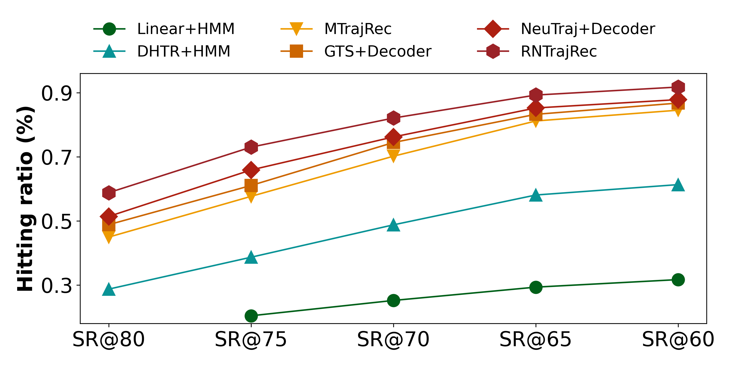
Figure 4: Performance evaluation for different methods on elevated road trajectory task (Chengdu: $\epsilon_{\tau}=\epsilon_{\rho}*8$).

Fig. 4 reports the experimental result for elevated road trajectory task on Chengdu dataset. We design this task to serve two main purposes. First, elevated roads and nearby trunk roads normally experience high traffic volume and their traffic conditions are typically more complicated (e.g., elevated roads are more likely to experience traffic congestion during peak hours). Therefore, evaluating the models’ ability to discover these sophisticated spatio-temporal patterns is significant. Second, the road network structure around the elevated road is more complex than other urban roads. For example, there are usually two-way trunk road segments under the elevated road segments, which brings greater challenges to the recovery of the road segments on these elevated roads.

As shown in Fig. 4, RNTrajRec significantly outperforms all the baseline models. Interestingly, all the learning-based models significantly outperform HMM-based methods (i.e. Linear/DHTR+HMM), which shows the inability of HMM to discover these complex patterns. In addition, our model can achieve a high F1 score ($>0.8$) for $58.8\%$ trajectories, which outperforms the best baseline by $14.4\%$.

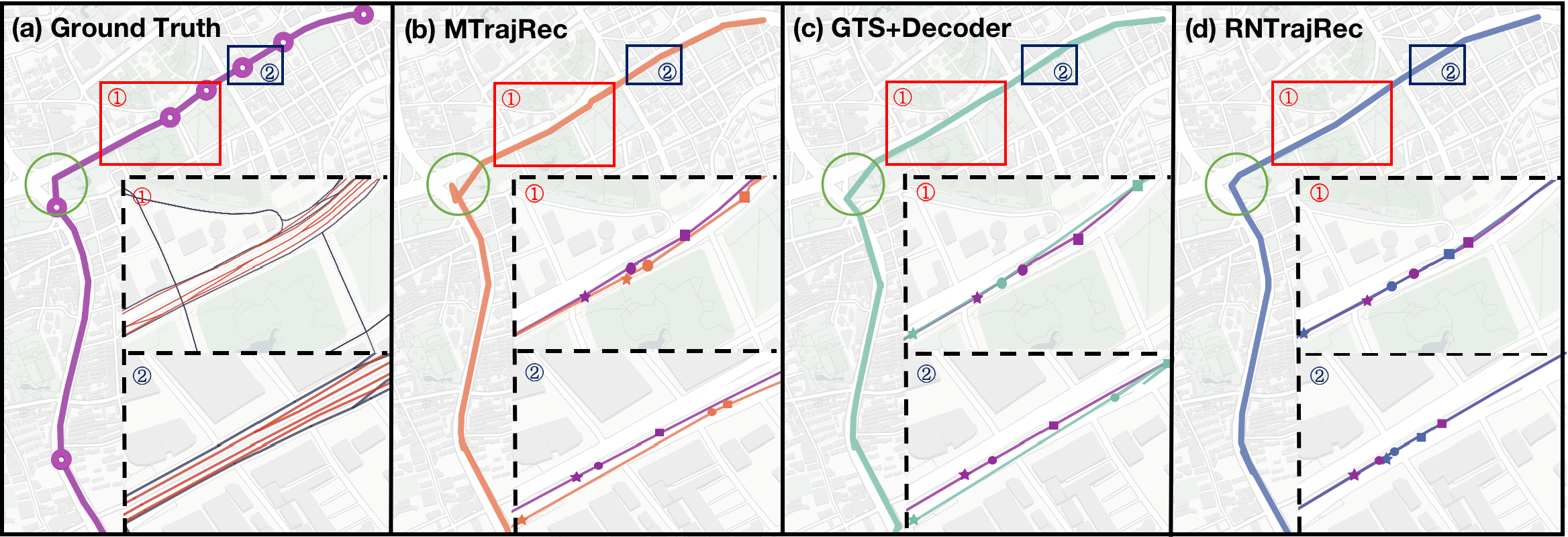
Figure 5: A case study for trajectory recovery. Purple circles in (a) represent the sample points in an input low sample trajectory. The red/black lines in dash-line rectangles of (a) represent the partial elevated/main road segments. The figures in the lower right corner of (b), (c), and (d) plot the detailed recovery results corresponding to the areas inside the red/black rectangles and the marker shapes indicate the sample timestamps (e.g., a purple star and an orange star in the dash-line rectangle labelled ② in (b) represent a point recovered by MTrajRec and the corresponding ground truth point of the same timestamp.)

VI-E Efficiency Study

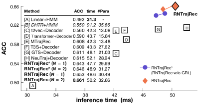
Figure 6: Efficiency study on Chengdu dataset ($\epsilon_{\tau}=\epsilon_{\rho}*8$)

.

In addition to the effectiveness of different methods, we also evaluate their efficiency by considering two different aspects, including inference time that refers to the time required to recover a trajectory during the inference phase and the number of parameters. As shown in Fig. 6, RNTrajRec requires less time during the inference than NeuTraj+Decoder, and comparable time cost against GTS+Decoder when using only one layer of GPSFormer. However, our model significantly outperforms both NeuTraj+Decoder and GTS+Decoder in terms of accuracy even if we set $N=1$. Besides, DHTR+HMM is observed to spend the most time during inference, probably due to the inefficiency of the adopted kalman filter module. Another observation is that Linear+HMM requires the least time during inference, however it suffers from low accuracy for trajectories with low sample rate. In short, RNTrajRec requires $50.2$ microseconds to recover a low-sample trajectory, which is efficient and practical in practice.

Remark: The time spent to obtain the road network representation via GridGNN is excluded from the inference time reported above. This is because the road network representation can be learned in advance as it is independent of the input trajectory used for the inference task.

VI-F Case Study

Fig. 5 visualizes trajectories recovered by different models, where the input trajectory is a low-sample elevated road trajectory. We sample partial underlying road network structures (e.g., elevated road segments represented by red lines and main road segments represented by black lines) in the two dash-line rectangles of Fig. 5(a). As we can observe from the visualization, the road network near the elevated roads is complicated. Purple lines in figures represent the ground truth trajectory and orange, green, blue-colored trajectories represent the trajectory recovered by MTrajRec, GTS+Decoder, and RNTrajRec respectively. We can observe that the trajectory recovered by our model matches the ground truth much better (e.g., the trajectories in the green circles provide one example), as RNTrajRec is able to capture the spatial and temporal patterns of trajectories in a more accurate manner. We further plot snapshots of two sections of restored trajectories (bounded by rectangles labelled ① and ②) by different models in the elevated road using the small pictures in the lower right corner in Fig. 5 (b)-(d), together with three recovered points from each section and their corresponding ground truth as examples. It can be observed that both road sections restored by MTrajRec and those restored by GTS+Decoder deviate from the ground truth, while the road sections restored by our model match the ground truth trajectory perfectly. In addition, we want to highlight that points recovered by the two baseline models lack spatial consistency due to their insufficient use of road network. For example, the orange/green star in Fig. 5 (b/c)-② is a point on the main road, while the next recovered point (i.e., the orange/green circle) is located on the elevated road. Although the two points seem to be located on the same road in our visualization, the shortest path distance between those two points is larger than $2000$ metres, implying that the recovered path between these two points is very different from the ground truth. In other words, the fact that our model can recover more accurate trajectories for elevated roads with complex network topology is significant.

TABLE V: Ablation studies on Chengdu and Porto datasets.

Variants	Chengdu ($\epsilon_{\tau}=\epsilon_{\rho}*8$)						Porto ($\epsilon_{\tau}=\epsilon_{\rho}*8$)
	Recall	Precision	F1 Score	Accuracy	MAE	RMSE	Recall	Precision	F1 Score	Accuracy	MAE	RMSE
w/o GRL	0.7696	0.8773	0.8177	0.6459	144.61	240.22	0.6671	0.7946	0.7227	0.5145	101.51	150.17
w/o GF	0.7725	0.8765	0.8191	0.6439	141.31	234.28	0.6697	0.7926	0.7234	0.5133	102.07	151.04
w/o GAT	0.7821	0.8729	0.8229	0.6292	144.70	237.82	0.6747	0.7962	0.7279	0.5195	98.65	147.98
w/o GN	0.7827	0.8672	0.8200	0.6306	146.56	241.25	0.6729	0.7951	0.7264	0.5171	99.84	148.05
w/o GCL	0.7773	0.8744	0.8209	0.6472	140.59	236.49	0.6683	0.7928	0.7227	0.5119	102.13	152.10
RNTrajRec	0.7831	0.8812	0.8272	0.6609	132.69	219.20	0.6778	0.7950	0.7293	0.5230	97.66	145.87

VI-G Ablation Study

To further prove the effectiveness of the modules proposed in the paper, we create five variants of RNTrajRec. w/o GRL replaces the graph refinement layer (GRL) in GPSFormer with standard transformer layer and ignores the graph structure input, i.e. $\widehat{G}_{\tau}$ and $\vec{Z}_{\tau}^{(0)}$; w/o GF replaces gated fusion discussed in Session IV-D1 with concatenation operation and feed forward network; w/o GN replaces graph normalization discussed in Session IV-D2 with standard layer normalization in transformer encoder; w/o GAT employs feed forward network but not graph attention network in graph refinement layer; w/o GCL removes graph classification (GCL) loss defined in Eq. (V). Experimental results are listed in Table V. We can observe that RNTrajRec consistently outperforms all its variants, which proves the significance of these modules.

As mentioned in Section IV-C, the local surrounding graph structure of GPS points is important for understanding the movement of a trajectory. Therefore, we observe a significant drop in overall performance after removing GRL, especially for Recall and F1 Score. Besides, we observe that RNTrajRec w/o GRL significantly outperforms Transformer+Decoder, with the input to the transformer layer being their only difference. Therefore, we conclude that a well-designed input embedding is significant for complex encoding models like transformer.

GRL is considered the most important component in RNTrajRec, in which graph normalization, gated fusion and graph forward is replaced with layer normalization, multi-head attention and feed forward network in original transformer respectively. In order to better justify the design of these individual modules, we design ablation study to answer the following three questions.

$\bullet$ Q1: Why we use graph normalization to replace layer normalization in graph refinement layer?

$\bullet$ Q2: Why we use graph attention network to replace feed forward network in graph refinement layer?

$\bullet$ Q3: Why we use gate fusion instead of other simple method (say concatenation or MLP) in graph refinement layer?

Q1: Why Graph Normalization? The idea of designing the graph normalization is inspired by [33], in which an experiment has been conducted to demonstrate that batch normalization is more suitable for graph transformers. Therefore, we design a similar normalization strategy for dynamic graph transformer (or spatial-temporal transformer). In addition, we observe that layer normalization ignores other nodes in the same sub-graph, which may cause the normalized features of different nodes in the same sub-graph lack discrimination.

Q2: Why Graph Attention Network? There are two main reasons behind the design of an additional graph attention network in graph refinement layer. First, as mentioned in Session IV-C, each subgraph $\vec{Z}_{\tau,i}^{(0)}$ directly uses the features in the road segments as the input but totally ignores the relationship inside each subgraph. Second, transformer encoder discussed in Session IV-E can effectively aggregate features from the entire trajectory, therefore, the relationship in each subgraph can be refined with the output of transformer encoder.

Q3: Why Gated Fusion? As mentioned in Session IV-D, we adopt gated fusion to adaptively fuse the input hidden vectors and the node features in the graph structure.

Extensive results reported in Table V well verify that the performance of RNTrajRec will degrade if any of the three parts are replaced/removed.

As for GCL, it is mainly to guide the process of trajectory encoding so as to generate more accurate trajectory representation. As shown in Table V, we observe that GCL indeed improves the accuracy of the recovered trajectory.

In addition, we study the effectiveness of different road network representation methods. As shown in Fig. 7(a), we compare GridGNN with three novel graph neural networks (GNNs), namely GCN, GIN and GAT for graph representation. All these models are implemented using standard DGL[60] library. We observe that GridGNN consistently performs the best, which shows the effectiveness of integrating grid information for road network representation. In addition, GAT outperforms GIN and GCN for graph representation, which shows the significance of self-attention mechanism.

VI-H Parameter Analysis

VI-H1 The impact of the number of GPSFormerBlock $N$

The number of GPSFormerBlock $N$ directly influences the complexity of RNTrajRec. To examine its impact, we vary $N$ in RNTrajRec from $1$ to $5$ and report the results in Fig. 7(b). Note, when $N$ is too large, the model will be more prone to overfitting, resulting in a decrease in its performance. We observe from the results that RNTrajRec achieves the highest accuracy when $N=3$. However, considering the efficiency of the model and the usage of GPU memory, we set $N$ to $2$.

VI-H2 The influence of receptive field of GPS point $\delta$

The value of receptive field of GPS point $\delta$ decides the size of the surrounding sub-graph of each GPS point in the trajectory. A larger $\delta$ allows the sub-graph to capture more information of surrounding area with a higher memory cost. In order to study the impact of $\delta$ on RNTrajRec’s performance, we vary $\delta$ from $100$ meters to $800$ meters. As shown in Fig. 7(c), RNTrajRec achieves the highest accuracy when $\delta$ is set to $600$ meters. To balance between the effectiveness and efficiency of the model, we set $\delta$ to $400$ meters.

VI-H3 The influence of hyper-parameter $\gamma$ in Eq. (5)

We vary the hyper-parameter $\gamma$ from $10$ meters to $50$ meters. With the increase of $\gamma$, the initial hidden-state vectors $H_{\tau}^{(0)}$ will pay more attention to the road segments that are closer to the GPS point, while pay less attention to those far away from the GPS point. Because of the uncertainty of GPS errors, the effect of increasing $\gamma$ on the model is also uncertain. As shown in Fig. 7(d), we observe that the performance of the model does not vary much as $\gamma$ changes. We believe the main reason is that GPSFormer can dynamically adjust the weight of each node in the sub-graph for the current GPS point, making the model insensitive to the changes of hyper-parameter $\gamma$.

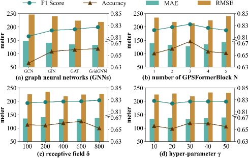
Figure 7: The performance of RNTrajRec on Chengdu dataset ($\epsilon_{\tau}=\epsilon_{\rho}*8$) under different hyper-parameters.

VI-I Discussion

We have explored many different techniques during the design of RNTrajRec. Though most of our attempts are effective, there is one technique that we tried but did not work. When designing the graph refinement layer, ideally the graph transformer network is able to refine not only the graph embedding of each subgraph but also the weight of each node in every subgraph. Specifically, we try to use the refined graph embedding at layer $l$, i.e. $\vec{Z}_{\tau}^{(l)}$, to obtain a new weight for each node by first transforming $\vec{Z}_{\tau}^{(l)}$, followed by either sigmoid function or softmax function. However, we find out that both sigmoid function and softmax function perform worse than a simple approach that does not refine the weight in each subgraph, i.e. directly using mean pooling as discussed in Section IV-D. We believe the main reason behind this failed attempt is that the linear transformation is too simple to learn valuable weights without proper supervision.

VII Conclusion

Trajectory recovery is a significant task for utilizing low-sample trajectories effectively. In this paper, we propose a novel spatial-temporal transformer-based model, namely RNTrajRec, to capture rich spatial and temporal information of the given low-sample trajectory. Specifically, we propose a road network representation module, namely GridGNN and a novel spatial-temporal transformer module, namely GPSFormer for encoding a GPS trajectory. We then forward the hidden-state vectors to a multi-task decoder model to recover the missing GPS points. Also, we propose a graph classification loss with constraint mask to guide the process of trajectory encoding. Extensive experiments on three real-life datasets show the effectiveness and efficiency of the proposed method.

VIII Acknowledgements

This research is supported in part by the National Natural Science Foundation of China under grant 62172107.

References

- [1] H. Zhang, H. Wu, W. Sun, and B. Zheng, “Deeptravel: a neural network based travel time estimation model with auxiliary supervision,” in Proceedings of the 27th International Joint Conference on Artificial Intelligence (IJCAI), 2018, pp. 3655–3661.
- [2] Y. Li, K. Fu, Z. Wang, C. Shahabi, J. Ye, and Y. Liu, “Multi-task representation learning for travel time estimation,” in Proceedings of the 24th ACM SIGKDD International Conference on Knowledge Discovery & Data Mining, 2018, pp. 1695–1704.
- [3] M. Li, P. Tong, M. Li, Z. Jin, J. Huang, and X.-S. Hua, “Traffic flow prediction with vehicle trajectories,” in Proceedings of the 35th AAAI Conference on Artificial Intelligence, vol. 35, no. 1, 2021, pp. 294–302.
- [4] C. Zheng, X. Fan, C. Wang, and J. Qi, “GMAN: A graph multi-attention network for traffic prediction,” in Proceedings of the 34th AAAI Conference on Artificial Intelligence, vol. 34, no. 01, 2020, pp. 1234–1241.
- [5] J. Jin, P. Cheng, L. Chen, X. Lin, and W. Zhang, “Gridtuner: Reinvestigate grid size selection for spatiotemporal prediction models,” in Proceedings of IEEE 38th International Conference on Data Engineering (ICDE). IEEE, 2022, pp. 1193–1205.
- [6] X. Li, K. Zhao, G. Cong, C. S. Jensen, and W. Wei, “Deep representation learning for trajectory similarity computation,” in Proceedings of IEEE 34th International Conference on Data Engineering (ICDE). IEEE, 2018, pp. 617–628.
- [7] D. Yao, G. Cong, C. Zhang, and J. Bi, “Computing trajectory similarity in linear time: A generic seed-guided neural metric learning approach,” in Proceedings of IEEE 35th Iinternational Conference on Data Engineering (ICDE). IEEE, 2019, pp. 1358–1369.
- [8] P. Yang, H. Wang, Y. Zhang, L. Qin, W. Zhang, and X. Lin, “T3S: effective representation learning for trajectory similarity computation,” in Proceedings of IEEE 37th International Conference on Data Engineering (ICDE). IEEE, 2021, pp. 2183–2188.
- [9] H. Zhang, X. Zhang, Q. Jiang, B. Zheng, Z. Sun, W. Sun, and C. Wang, “Trajectory similarity learning with auxiliary supervision and optimal matching,” in Proceedings of the 29th International Joint Conference on Artificial Intelligence (IJCAI), 2020, pp. 3209–3215.
- [10] P. Han, J. Wang, D. Yao, S. Shang, and X. Zhang, “A graph-based approach for trajectory similarity computation in spatial networks,” in Proceedings of the 27th ACM SIGKDD Conference on Knowledge Discovery & Data Mining, 2021, pp. 556–564.
- [11] H. Ren, S. Ruan, Y. Li, J. Bao, C. Meng, R. Li, and Y. Zheng, “MTrajRec: Map-constrained trajectory recovery via seq2seq multi-task learning,” in Proceedings of the 27th ACM SIGKDD Conference on Knowledge Discovery & Data Mining, 2021, pp. 1410–1419.
- [12] K. Zhao, J. Feng, Z. Xu, T. Xia, L. Chen, F. Sun, D. Guo, D. Jin, and Y. Li, “DeepMM: Deep learning based map matching with data augmentation,” in Proceedings of the 27th ACM SIGSPATIAL International Conference on Advances in Geographic Information Systems, 2019, pp. 452–455.
- [13] J. Yuan, Y. Zheng, C. Zhang, X. Xie, and G.-Z. Sun, “An interactive-voting based map matching algorithm,” in Proceedings of the 11th Eleventh International Conference on Mobile Data Management. IEEE, 2010, pp. 43–52.
- [14] P. Newson and J. Krumm, “Hidden markov map matching through noise and sparseness,” in Proceedings of the 17th ACM SIGSPATIAL International Conference on Advances in Geographic Information Systems, 2009, pp. 336–343.
- [15] Y. Lou, C. Zhang, Y. Zheng, X. Xie, W. Wang, and Y. Huang, “Map-matching for low-sampling-rate gps trajectories,” in Proceedings of the 17th ACM SIGSPATIAL International Conference on Advances in Geographic Information Systems, 2009, pp. 352–361.
- [16] G. R. Jagadeesh and T. Srikanthan, “Online map-matching of noisy and sparse location data with hidden markov and route choice models,” IEEE Transactions on Intelligent Transportation Systems, vol. 18, no. 9, pp. 2423–2434, 2017.
- [17] R. Song, W. Lu, W. Sun, Y. Huang, and C. Chen, “Quick map matching using multi-core cpus,” in Proceedings of the 20th International Conference on Advances in Geographic Information Systems, 2012, pp. 605–608.
- [18] S. Hoteit, S. Secci, S. Sobolevsky, C. Ratti, and G. Pujolle, “Estimating human trajectories and hotspots through mobile phone data,” Computer Networks, vol. 64, pp. 296–307, 2014.
- [19] J. Wang, N. Wu, X. Lu, W. X. Zhao, and K. Feng, “Deep trajectory recovery with fine-grained calibration using kalman filter,” IEEE Transactions on Knowledge and Data Engineering, vol. 33, no. 3, pp. 921–934, 2019.
- [20] I. Sutskever, O. Vinyals, and Q. V. Le, “Sequence to sequence learning with neural networks,” Advances in Neural Information Processing Systems, vol. 27, pp. 3104–3112, 2014.
- [21] K. Cho, B. Van Merriënboer, D. Bahdanau, and Y. Bengio, “On the properties of neural machine translation: Encoder-decoder approaches,” arXiv preprint arXiv:1409.1259, 2014.
- [22] A. Vaswani, N. Shazeer, N. Parmar, J. Uszkoreit, L. Jones, A. N. Gomez, Ł. Kaiser, and I. Polosukhin, “Attention is all you need,” Advances in Neural Information Processing Systems, vol. 30, pp. 5998–6008, 2017.
- [23] J. Devlin, M.-W. Chang, K. Lee, and K. Toutanova, “BERT: Pre-training of deep bidirectional transformers for language understanding,” Proceedings of the 2019 Conference of the North American Chapter of the Association for Computational Linguistics: Human Language Technologies, (NAACL-HLT), pp. 4171–4186, 2019.
- [24] X. Liu, Y. Zheng, Z. Du, M. Ding, Y. Qian, Z. Yang, and J. Tang, “GPT understands, too,” arXiv preprint arXiv:2103.10385, 2021.
- [25] N. Carion, F. Massa, G. Synnaeve, N. Usunier, A. Kirillov, and S. Zagoruyko, “End-to-end object detection with transformers,” in Proceedings of the 16th European Conference on Computer Vision, vol. 12346. Springer, 2020, pp. 213–229.
- [26] Z. Liu, Y. Lin, Y. Cao, H. Hu, Y. Wei, Z. Zhang, S. Lin, and B. Guo, “Swin Transformer: Hierarchical vision transformer using shifted windows,” in Proceedings of the IEEE/CVF International Conference on Computer Vision, 2021, pp. 10 012–10 022.
- [27] Y. Fang, B. Liao, X. Wang, J. Fang, J. Qi, R. Wu, J. Niu, and W. Liu, “You only look at one sequence: Rethinking transformer in vision through object detection,” Advances in Neural Information Processing Systems, vol. 34, pp. 26 183–26 197, 2021.
- [28] I. Beltagy, M. E. Peters, and A. Cohan, “Longformer: The long-document transformer,” arXiv preprint arXiv:2004.05150, 2020.
- [29] H. Zhou, S. Zhang, J. Peng, S. Zhang, J. Li, H. Xiong, and W. Zhang, “Informer: Beyond efficient transformer for long sequence time-series forecasting,” in Proceedings of the 35th AAAI Conference on Artificial Intelligence, 2021, pp. 11 106–11 115.
- [30] N. Kitaev, Ł. Kaiser, and A. Levskaya, “Reformer: The efficient transformer,” in Proceedings of the 8th International Conference on Learning Representations (ICLR), 2020.
- [31] S. Yun, M. Jeong, R. Kim, J. Kang, and H. J. Kim, “Graph transformer networks,” Advances in Neural Information Processing Systems, vol. 32, pp. 11 960–11 970, 2019.
- [32] D. Cai and W. Lam, “Graph transformer for graph-to-sequence learning,” in Proceedings of the 34th AAAI Conference on Artificial Intelligence, vol. 34, no. 05, 2020, pp. 7464–7471.
- [33] V. P. Dwivedi and X. Bresson, “A generalization of transformer networks to graphs,” arXiv preprint arXiv:2012.09699, 2020.
- [34] C. Yu, X. Ma, J. Ren, H. Zhao, and S. Yi, “Spatio-temporal graph transformer networks for pedestrian trajectory prediction,” in Proceedings of the 16th European Conference on Computer Vision. Springer, 2020, pp. 507–523.
- [35] Y. Cong, W. Liao, H. Ackermann, B. Rosenhahn, and M. Y. Yang, “Spatial-temporal transformer for dynamic scene graph generation,” in Proceedings of the IEEE/CVF International Conference on Computer Vision, 2021, pp. 16 372–16 382.
- [36] C. Zheng, S. Zhu, M. Mendieta, T. Yang, C. Chen, and Z. Ding, “3d human pose estimation with spatial and temporal transformers,” in Proceedings of the IEEE/CVF International Conference on Computer Vision, 2021, pp. 11 656–11 665.
- [37] S. Li, Q. Cao, L. Liu, K. Yang, S. Liu, J. Hou, and S. Yi, “Groupformer: Group activity recognition with clustered spatial-temporal transformer,” in Proceedings of the IEEE/CVF International Conference on Computer Vision, 2021, pp. 13 668–13 677.
- [38] Y. Zhang, B. Wu, W. Li, L. Duan, and C. Gan, “Stst: Spatial-temporal specialized transformer for skeleton-based action recognition,” in Proceedings of the 29th ACM International Conference on Multimedia, 2021, pp. 3229–3237.
- [39] A. Grover and J. Leskovec, “node2vec: Scalable feature learning for networks,” in Proceedings of the 22nd ACM SIGKDD International Conference on Knowledge Discovery and Data Mining, 2016, pp. 855–864.
- [40] B. Perozzi, R. Al-Rfou, and S. Skiena, “Deepwalk: Online learning of social representations,” in Proceedings of the 20th ACM SIGKDD International Conference on Knowledge Discovery and Data Mining, 2014, pp. 701–710.
- [41] T. N. Kipf and M. Welling, “Semi-supervised classification with graph convolutional networks,” in Proceedings of 5th International Conference on Learning Representations (ICLR), Conference Track Proceedings, 2017.
- [42] W. Hamilton, Z. Ying, and J. Leskovec, “Inductive representation learning on large graphs,” Advances in Neural Information Processing Systems, vol. 30, pp. 1024–1034, 2017.
- [43] P. Veličković, G. Cucurull, A. Casanova, A. Romero, P. Lio, and Y. Bengio, “Graph attention networks,” in Proceedings of 6th International Conference on Learning Representations (ICLR), Conference Track Proceedings, 2018.
- [44] K. Xu, W. Hu, J. Leskovec, and S. Jegelka, “How powerful are graph neural networks?” in Proceedings of 7th International Conference on Learning Representations (ICLR), 2019.
- [45] G. Jin, H. Yan, F. Li, J. Huang, and Y. Li, “Spatio-temporal dual graph neural networks for travel time estimation,” arXiv preprint arXiv:2105.13591, 2021.
- [46] N. Wu, X. W. Zhao, J. Wang, and D. Pan, “Learning effective road network representation with hierarchical graph neural networks,” in Proceedings of the 26th ACM SIGKDD International Conference on Knowledge Discovery & Data Mining, 2020, pp. 6–14.
- [47] Y. Chen, X. Li, G. Cong, Z. Bao, C. Long, Y. Liu, A. K. Chandran, and R. Ellison, “Robust road network representation learning: When traffic patterns meet traveling semantics,” in Proceedings of the 30th ACM International Conference on Information & Knowledge Management, 2021, pp. 211–220.
- [48] S. Hochreiter and J. Schmidhuber, “Long short-term memory,” Neural Computation, vol. 9, no. 8, pp. 1735–1780, 1997.
- [49] T. Xia, Y. Qi, J. Feng, F. Xu, F. Sun, D. Guo, and Y. Li, “AttnMove: History enhanced trajectory recovery via attentional network,” in Proceedings of the 35th AAAI Conference on Artificial Intelligence, vol. 35, no. 5, 2021, pp. 4494–4502.
- [50] D. Xi, F. Zhuang, Y. Liu, J. Gu, H. Xiong, and Q. He, “Modelling of bi-directional spatio-temporal dependence and users’ dynamic preferences for missing poi check-in identification,” in Proceedings of the 33rd AAAI Conference on Artificial Intelligence, vol. 33, no. 01, 2019, pp. 5458–5465.
- [51] A. Guttman, “R-trees: A dynamic index structure for spatial searching,” in Proceedings of ACM SIGMOD International Conference on Management of Data, 1984, pp. 47–57.
- [52] S. Ioffe and C. Szegedy, “Batch Normalization: Accelerating deep network training by reducing internal covariate shift,” in Proceedings of the 32nd International Conference on Machine Learning (ICML). PMLR, 2015, pp. 448–456.
- [53] Z. Fang, Y. Du, X. Zhu, D. Hu, L. Chen, Y. Gao, and C. S. Jensen, “Spatio-temporal trajectory similarity learning in road networks,” in Proceedings of the 28th ACM SIGKDD Conference on Knowledge Discovery and Data Mining, 2022, pp. 347–356.
- [54] G. Cui, J. Luo, and X. Wang, “Personalized travel route recommendation using collaborative filtering based on gps trajectories,” International Journal of Digital Earth, vol. 11, no. 3, pp. 284–307, 2018.
- [55] T. Kurashima, T. Iwata, G. Irie, and K. Fujimura, “Travel route recommendation using geotags in photo sharing sites,” in Proceedings of the 19th ACM International Conference on Information and Knowledge Management, 2010, pp. 579–588.
- [56] D. Iland, A. Irish, U. Madhow, and B. Sandler, “Rethinking gps: Engineering next-gen location at uber,” Retrieved from Uber Engineering: https://eng. uber. com/rethinking-gps, 2018.
- [57] A. Paszke, S. Gross, F. Massa, A. Lerer, J. Bradbury, G. Chanan, T. Killeen, Z. Lin, N. Gimelshein, L. Antiga et al., “Pytorch: An imperative style, high-performance deep learning library,” Advances in Neural Information Processing Systems, vol. 32, pp. 8024–8035, 2019.
- [58] D. P. Kingma and J. Ba, “Adam: A method for stochastic optimization,” arXiv preprint arXiv:1412.6980, 2014.
- [59] R. E. Kalman, “A new approach to linear filtering and prediction problems,” 1960.
- [60] M. Wang, D. Zheng, Z. Ye, Q. Gan, M. Li, X. Song, J. Zhou, C. Ma, L. Yu, Y. Gai et al., “Deep graph library: A graph-centric, highly-performant package for graph neural networks,” arXiv preprint arXiv:1909.01315, 2019.