Abstract

A biological system is a complex network of heterogeneous molecular entities and their interactions contributing to various biological characteristics of the system. However, current biological networks are noisy, sparse, and incomplete, limiting our ability to create a holistic view of the biological system and understand the biological phenomena. Experimental identification of such interactions is both time-consuming and expensive. With the recent advancements in high-throughput data generation and significant improvement in computational power, various computational methods have been developed to predict novel interactions in the noisy network. Recently, deep learning methods such as graph neural networks have shown their effectiveness in modeling graph-structured data and achieved good performance in biomedical interaction prediction. However, graph neural networks-based methods require human expertise and experimentation to design the appropriate complexity of the model and significantly impact the performance of the model. Furthermore, deep graph neural networks face overfitting problems and tend to be poorly calibrated with high confidence on incorrect predictions. To address these challenges, we propose Bayesian model selection for graph convolutional networks to jointly infer the most plausible number of graph convolution layers (depth) warranted by data and perform dropout regularization simultaneously. Experiments on four interaction datasets show that our proposed method achieves accurate and calibrated predictions. Our proposed method enables the graph convolutional networks to dynamically adapt their depths to accommodate an increasing number of interactions.

Introduction

Biomedical interaction networks represent the complex interplay between heterogeneous molecular entities such as genes, proteins, drugs, and diseases within a biological system. The study of interaction networks advances our understanding of system-level understanding of biology [1] and the discovery of biologically significant novel interactions including protein-protein interactions (PPIs) [2], drug-drug interactions (DDIs) [3], drug-target interactions (DTIs) [4] and gene-disease associations (GDIs) [5]. There have been huge technological advancements in high-throughput technologies that have produced an ever-increasing amount of omics data and resulted in the identification of novel interactions. Despite this, current biological networks are noisy, sparse, and incomplete, which limits our ability to study the biological phenomena at the system level.

Various computational methods have been developed to predict novel interactions in biomedical interaction networks. In particular, various network-based approaches have been proposed to exploit already available interactions to predict missing interactions . The higher similarity of network properties between the biological entities is considered as an indication of interaction. Specifically, the Triadic closure principle (TCP) indicates that biological entities with shared neighbors are likely to interact with each other . However, the common neighbor hypothesis fails to identify novel interactions between most protein pairs in PPI prediction. To solve this, L3 heuristic [6] suggests that biological entities linked by multiple paths of length 3 are more likely to have direct links/interactions.

Alternatively, network embedding approaches such as Deepwalk [7], node2vec [8] propose to embed the nodes in the network to a low-dimensional vector representation that preserves the network properties. Deepwalk [7] generates the truncated random walks of length $l$ and defines a context window of size $k$ as a neighborhood for each node. Distributed representation for each node in the network is learned based on random walks. However, Deepwalk relies on the rigid notion of network neighborhood that makes it largely insensitive to the connectivity patterns unique to the network. node2vec defines a flexible notion of node’s network neighborhood by performing a biased random walk by balancing breadth-first and depth-first search in the network. These network embedding methods generate feature representations that maximize the likelihood of preserving the network neighborhood of nodes in a low-dimensional feature space. A classifier is trained on these embeddings to predict the interaction probability. These methods are only limited to the structure of the biological networks and cannot integrate the features of biological nodes.

Recently, deep learning approaches on network datasets have shown great success across various domains such as social networks [9], recommendation systems [10], chemistry [11], citation networks [12]. Specifically, graph convolutional networks (GCNs) have shown great success in biomedical interaction prediction [13, 14]. GCN-based methods follow a message passing mechanism that recursively receives and aggregates information from its neighbors and transform the representation of the biological nodes in the network. $L$ layers of GCN-based models represent $L$ iterations of the neighborhood aggregation scheme such that each node in the biological network captures the network topological information within its $L$-hop neighborhood. A higher-order neighborhood might be informative to provide the model with more topological information, especially for nodes in an incomplete and sparse network. To this end, higher-order GCN models were proposed [14].

Despite the enormous success of GCN models in biomedical interaction prediction, the neural network structure (number of layers and number of neurons in each layer) of GCN models is a critical choice and needs to be carefully set. Most of the recent GCN models such as GCN [15] and GAT [16] define shallow network structures (i.e., 2-layer models) to achieve their best performance. The ability of GCN models with shallow structures is limited and fails to extract information from higher-order neighbors. Although stacking multiple GCN layers and non-linearity enable the model to capture information from higher-order neighbors, such deep GCN models tend to face the over-smoothing problem as the performance of deep models degrades with the increase in the number of layers [15]. In particular, 2-layered GCN and GAT models outperform deep models.

To address the challenge, we propose Bayesian model selection [17] to jointly infer the depth of GCN models warranted by data and perform dropout regularization simultaneously [17]. To enable the number of GCN layers in the encoder to go to infinity in theory, we model the depth of GCN models as a stochastic process by defining the beta process over the number of GCN layers. The beta process induces layer-wise activation probabilities that modulate neuron activations for regularization via a conjugate Bernoulli process. The proposed framework balances the GCN model’s depth and neuron activations and provides well-calibrated predictions.

We evaluate the performance of our inference framework and compare it with GCN-based models for biomedical interaction prediction. We demonstrate that the GCN-based encoder suffers from the over-fitting problem as the depth increases but our model infers the most plausible depth and is quite robust to the overfitting problem. Furthermore, experiments on sparse interaction networks with an increasing number of interactions show that our method achieves superior performance by enabling the structure of the GCN-based encoder to dynamically evolve to accommodate incrementally available information.

In summary, our contributions are as follows:

• We propose a Bayesian model selection to jointly infer the most plausible depth and their neuron activations for encoder warranted by data simultaneously to learn representation for biomedical entities.

• We empirically demonstrate that our inference framework achieves superior performance by dynamically balancing the neural network depth and their neuron activation for the encoder.

• Our method enables the structure of the encoder to dynamically evolve to accommodate the information from an increasing number of interactions.

• We further show that our method is capable of making novel predictions that are validated using up-to-date literature-based database entries.

Materials and methods

Biomedical interaction prediction

A biomedical network is a network with biomedical entities as nodes and their interactions as edges. Formally, a biomedical network can be defined as $\mathcal{G}=(\mathcal{V},\mathcal{E},\mathbf{X})$ where $\mathcal{V}$ denotes the set of nodes representing biomedical entities such as proteins, genes, drugs, diseases and $\mathcal{E}$ represents the set of interaction between these entities. We denote the network $\mathcal{G}$ with an adjacency matrix $\mathbf{A}$ where $A_{ij}$ represents the presence or absence of an edge between nodes. We consider the binary adjacency matrix $A_{ij}\in\{0,1\}^{|\mathcal{V}|\times|\mathcal{V}|}$. In particular, $A_{ij}=1$ represents the existence of an interaction supported by experimental evidence whereas $A_{ij}=0$ represents the absence of interaction.

Biomedical interaction prediction: Given a biomedical interaction network $\mathcal{G}=(\mathcal{V},\mathcal{E},\mathbf{X})$, we aim to learn a model $f$ to predict the probability of interaction $e_{ij}$ between nodes in the network: $\phi:e_{ij}\rightarrow[0,1]$.

Graph convolution-based encoder-decoder framework

In this work, we closely follow the encoder-decoder framework [18] to learn the node representation of biological networks. First, an encoder model maps each node in the biological network into a low-dimensional representation. Next, a decoder model reconstructs the structural information about the biological network from the learned representations.

Formally, an encoder is a function that maps the biological entities $v\in\mathcal{V}$ to low-dimensional vector representation $\mathbf{q}\in\mathbb{R}^{M}$:

$$\text{ENC}:\mathcal{V}\rightarrow\mathbb{R}^{M}$$ (1)

Recently, graph neural network models have been proposed to generate representations of nodes that depend on the structure of the graph and feature information. In particular, the Graph convolution (GC) layer [15] generates representation for nodes in the network by repeatedly aggregating information from immediate neighbors. GC layer can be defined as:

$$\mathbf{H}_{l}=\sigma(\widehat{\mathbf{A}}\mathbf{H}_{l-1}\mathbf{W}_{l})$$ (2)

where $\widehat{\mathbf{A}}$ is a symmetrically normalized adjacency matrix with self-connections $\widehat{\mathbf{A}}=\mathbf{D}^{-\frac{1}{2}}(\mathbf{A}+\mathbf{I}_{|\mathcal{V}|})\mathbf{D}^{-\frac{1}{2}}$. Let $\mathbf{W}_{l}$ is a trainable weight matrix for layer $l$, $\mathbf{H}_{l-1}$ and $\mathbf{H}_{l}$ are the input and output activations respectively. We can then define a GCN model with $L$ layers can be defined as:

$$\mathbf{H}^{(l)}=\begin{cases}\mathbf{X}&\text{if $l=0$}\\ \sigma(\widehat{\mathbf{A}}\mathbf{H}_{l-1}\mathbf{W}_{l})&\text{if $l\in[1,\ldots,L]$}\end{cases}$$ (3)

$\mathbf{H}_{L}\in\mathbb{R}^{|\mathcal{V}|\times M}$ represents the representation for each entity in the network. We denote this representation as $\mathbf{Q}$. $L$ layers of GC layer aggregate the network topological information from $L$-hop neighborhood.

The decoder uses the representation generated by the encoder and reconstructs the structural properties of the biological network. For interaction prediction, a pairwise decoder is defined to predict the relationship or similarity between pairs of nodes:

$$\text{DEC}:\mathbb{R}^{M}\times\mathbb{R}^{M}\rightarrow\mathbb{R}^{+}$$ (4)

Probabilistic model selection for graph convolution-based encoder

In this work, we propose a probabilistic model selection [17] to infer the depth and neurons activations of graph convolutional encoder to learn the representation for each entity in the network. In addition, we employ a bilinear decoder to reconstruct the edges in the interaction network [14]. We adopt the encoder-decoder framework for biomedical interaction prediction [14]. Figure 1 shows the block diagram of the model.

• Encoder: a graph convolution encoder with potentially infinite hidden layers that takes an interaction graph $\mathcal{G}$ and generates representation for each entity in the interaction network. In particular, we propose to model the depth of graph convolution encoder as a stochastic process and jointly perform dropout regularization upon the inferred hidden layers.

• Decoder: a bilinear decoder that takes the representation of two nodes $v_{i}$ and $v_{j}$ and compute the probability $p_{ij}$ of their interaction $e_{ij}$.

We next discuss the details of each component of the proposed framework.

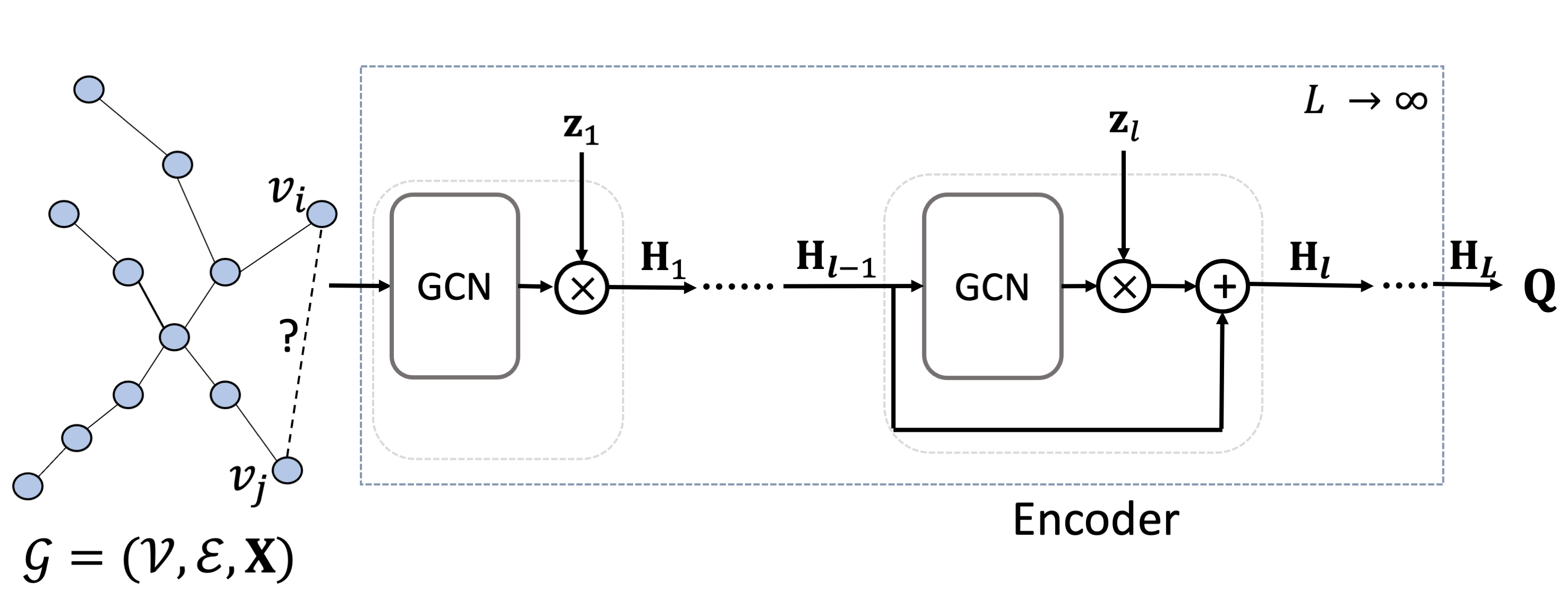
Fig 1: The block diagram of our proposed model with potentially infinite number of hidden layers in encoder. The input to the network is a biomedical interaction network $\mathcal{G}$ with edges $\mathcal{E}$ between entities $\mathcal{V}$ and feature matrix $\mathbf{X}$. The encoder with infinite hidden layers learns the final representation $\mathbf{Q}$. We use the bilinear decoder [14] that takes the representation $(\mathbf{q}_{i},\mathbf{q}_{j})$ for two entities $(v_{i},v_{j})$ and predict the probability $p_{ij}$ of their interaction based on the edge representation $\mathbf{e}_{ij}$.

Graph convolutional encoder with infinite layers

Deep GC encoder faces the issue of overfitting such that 2-layer models perform better than deeper models [15]. The depth ($L$) of the GC encoder is a critical choice and needs to be carefully set. To address this challenge, we propose to model the depth of the encoder as a stochastic process by defining a beta process over the hidden layers [19, 20, 17]. We adopt the stick-breaking construction of the beta-Bernoulli process as:

$$z_{ml}\sim\text{Bernoulli}(\pi_{l}),\quad\pi_{l}=\prod_{j=1}^{l}\nu_{j},\quad\nu_{l}\sim\text{Beta}(\alpha,\beta)$$ (5)

where $\nu_{l}$ are sequentially drawn from beta distribution and $\pi_{l}$ represents the activation probability of layer $l$ that decreases with layer $l$. $z_{ml}$ represents Bernoulli variable with a probability that $z_{ml}=1$ equals to $\pi_{l}$. Specifically, $z_{ml}=1$ indicates that $m$’th neuron in layer $l$ is activated. With beta process over the hidden layers, the GC encoder takes the form:

$$\mathbf{H}_{l}=\sigma(\widehat{\mathbf{A}}\mathbf{H}_{l-1}\mathbf{W}_{l})\bigotimes\mathbf{z}_{l}+\mathbf{H}_{l-1},\quad l\in\{1,2,\ldots\infty\}$$ (6)

where $\mathbf{W}_{l}\in\mathbb{R}^{M\times M}$ is the weight matrix of layer $l$. We regularize the output of layer $l$ by multiplying it elementwisely by a binary vector $\mathbf{z}_{l}$ where its element $z_{ml}\in\{0,1\}$. Figure 1 shows the network structure with binary vector $\mathbf{z}_{l}$ applied to the output of layer $l$ and skip connection.

Bilinear interaction decoder

We adopt bilinear decoder [14] to use representations obtained from the encoder and predict the probability of interactions between biomedical entities. Specifically, we define a bilinear layer that maps the representation of entities $\mathbf{q}_{i}\in\mathbb{R}^{M\times 1}$ and $\mathbf{q}_{j}\in\mathbb{R}^{M\times 1}$ to their edge representation $\mathbf{e}_{ij}\in\mathbb{R}^{d^{*}\times 1}$ as:

$$\mathbf{e}_{ij}=\text{ELU}(\mathbf{q}_{i}\mathbf{W}_{b}\mathbf{q}_{j}+\mathbf{b})$$ (7)

where $\mathbf{e}_{ij}$ denotes the representation of edge between entities $v_{i}$ and $v_{j}$, $\mathbf{W}_{b}\in\mathbb{R}^{d^{*}\times M\times M}$ represents the learnable fusion matrix, and $\mathbf{b}$ denotes the bias of bilinear layer. The probability $p_{ij}$ of interaction between entities $v_{i}$ and $v_{j}$ is obtained by passing the edge representation $\mathbf{e}_{ij}$ through the fully-connected (FC) layer.

$$p_{ij}=\text{sigmoid}(\text{FC}_{2}(\text{ELU}(\text{FC}_{1}(\mathbf{e}_{ij})))$$ (8)

Efficient variational approximation

Given an interaction dataset $D=\{\mathbf{A},\mathbf{X}\}$ with adjacency matrix $\mathbf{A}\in\mathbb{R}^{|\mathcal{V}|\times|\mathcal{V}|}$ and feature matrix $\mathbf{X}$, we aim to reconstruct the edges in the input network. For the problem of classifying the edges, we express the likelihood of the neural network as:

$$p(D|\mathbf{Z},\mathbf{W})=\prod_{n=1}^{N}\text{Bernoulli}(A_{ij}|f(\mathbf{A},\mathbf{X};\mathbf{Z},\mathbf{W}))$$ (9)

where $f(\cdot)$ represents the softmax function, $\mathbf{Z}$ is a binary matrix that represents the network structure for GC encoder whose $l$-th column is $\mathbf{z}_{l}$, and $\mathbf{W}$ denotes the set of weight matrices.

We define a prior over network structure $\mathbf{Z}$ via beta process as

$$p(\mathbf{Z},\mathbf{\nu}|\alpha,\beta) =p(\mathbf{\nu}|\alpha,\beta)p(\mathbf{Z}|\mathbf{\nu})$$

$$=\prod_{l=1}^{\infty}\text{Beta}(\nu_{l}|\alpha,\beta)\text{Bernoulli}(z_{ml}|\pi_{l})$$ (10)

The marginal likelihood obtained by combining beta process prior in Equation Efficient variational approximation and the likelihood in Equation 9 is:

$$p(D|\mathbf{W},L,\alpha,\beta)=\int p(D|\mathbf{W},\mathbf{Z})p(\mathbf{Z},\nu|\alpha,\beta)d\mathbf{Z}d\mathbf{\nu}$$ (11)

The exact computation of marginal likelihood is intractable because of the non-linearity of the neural network and $L\rightarrow\infty$.

We then use a structured stochastic variational inference framework introduced by [21, 22] to approximate the marginal likelihood. The lower bound for log marginal likelihood is:

$$\log p(D|\mathbf{W},L,\alpha,\beta) \geq\mathbb{E}_{q(\mathbf{Z},\nu)]}[\log p(D|\mathbf{W},\mathbf{Z})]-\text{KL}[q(\nu)||p(\nu)]$$

$$-\text{KL}[q(\mathbf{Z}|\nu)||p(\mathbf{Z}|\nu)]$$ (12)

where $q(\nu)$ and $q(\mathbf{Z}|\nu)$ represent variational beta distribution and variational Bernoulli distribution resepectively. Formally, we define $q(\nu)=\text{Beta}(\nu_{k}|a_{k},b_{k})$ with $a_{k}$ and $b_{k}$ as variational parameters. We next define $q(\mathbf{Z}|\nu))=\text{ConcreteBernoulli}(z_{mk}|\pi_{k})$. For variational approximation, we use truncation level $K$ to denote potentially infinite number of layers.

Training algorithm

Our proposed framework leverages biomedical interaction network $\mathbf{A}$ and feature representation of biomedical entities $\mathbf{X}$. For all experiments, we set $\mathbf{X}$ to be one-hot encoding $\mathbf{I}_{|\mathcal{V}|}$. If features are available for biomedical entities, we can initialize $\mathbf{X}$ accordingly. We can also initialize the feature matrix using pre-trained embeddings from other network embedding approaches such as DeepWalk, node2vec.

To compute the expectation in Equation Efficient variational approximation, we make Monte-Carlo estimation with $S$ samples of encoder structure $Z$ (depth of the encoder with layer-wise activation probabilities). The stick-breaking construction of beta-Bernoulli process induces that the probability of being activated in hidden layer $l$ decreases exponentially with $K$. With a large $K$, a small number of hidden layers in the encoder has activated neurons which can be obtained as

$$l^{c}=\text{max}_{l}\{l|\sum_{m=1}^{M}z_{ml}>1\}$$ (13)

where $\sum_{m=1}^{M}z_{ml}$ represents total activation of neurons in layer $l$. We can compute the expectation of log-likelihood based on $S$ samples of encoder structure:

$$\mathbb{E}_{q(Z,v)}[\log p(D|\mathbf{Z},\nu)]=\frac{1}{S}[\log p(D|\mathbf{Z}_{s},\nu)]$$ (14)

We summarize the algorithm to train our proposed framework in Algorithm 1.

Algorithm 1 Training of our proposed method

Input $\{D_{i}\}_{i=1}^{B}$: $B$ mini batches of interaction data
Input $S$: the number of samples of encoder structures $\mathbf{Z}$

1:  for $\text{i}=1,\ldots,B$ do

2:     Draw $S$ samples of encoder structures $\{\mathbf{Z}_{s}\}_{s=1}^{S}$ from $q(\mathbf{Z},\boldsymbol{\nu})$

3:     for $\text{s}=1,\ldots,S$ do

4:        Compute the number of layers $l^{c}$ from $\mathbf{Z}_{s}$ using (13)

5:        Compute $\log p(D_{i}|\mathbf{Z}_{s},\mathbf{W})$ with $l^{c}$ layers

6:     end for

7:     Compute $\mathbb{E}_{q(\mathbf{Z},\boldsymbol{\nu})}[\log p(D_{i}|\mathbf{Z},\mathbf{W})]$ using (14)

8:     Compute ELBO using (Efficient variational approximation)

9:     Update $\{{a_{k}},{b_{k}}\}_{k=1}^{l^{c}}$and $\{{\mathbf{W}}\}_{k=1}^{l^{c}}$ using backpropagation

10:  end for

The parameters of our proposed framework are learned by optimizing the ELBO in Equation Efficient variational approximation in an end-to-end manner. With the trained model, we can predict the probability of interaction between any pair of entities in the interaction network.

Results and discussion

We evaluate the performance of our proposed framework by applying it to infer the neural network structure for graph convolutional encoder on biomedical interaction prediction. We investigate our method’s performance and compare it with the heuristically designed encoder structure. We further demonstrate that the settings of truncation have no impact on the performance of our model.

Datasets

For experimental evaluation, we consider four publicly-available biological network datasets: (a) BioSNAP-DTI: Drug Target interaction network with 15,139 drug-target interactions between 5,018 drugs and 2,325 proteins, (b) BioSNAP-DDI: Drug-Drug interactions with 48,514 drug-drug interactions between 1,514 drugs extracted from drug labels and biomedical literature, (c) HuRI-PPI: HI-III human PPI network contains 5,604 proteins and 23,322 interactions generated by multiple orthogonal high-throughput yeast two-hybrid screens. and (d) DisGeNET-GDI: gene-disease network with 81,746 interactions between 9,413 genes and 10,370 diseases curated from GWAS studies, animal models, and scientific literature. For all interaction datasets, we represent the interactions as binary adjacency matrix $\mathbf{A}$ with $0$ representing the absence of interactions and $1$ representing the presence of interactions.

Baselines

We compare our proposed method with the following baselines for interaction prediction.

• DeepWalk [7] performs truncated random walk exploring the network neighborhood of nodes and applies the skip-gram model to learn the $M$-dimensional embedding for each node in the network. Node features are concatenated to form edge representation and a logistic regression classifier is trained.

• node2vec [8] extends DeepWalk by running biased random walk based on breadth/depth-first search to capture both local and global network structure.

• L3 [6] counts the number of length 3 paths normalized by the degree for all the node pairs.

• GCN [15] uses normalized adjacency matrix to learn node representations. The representation for nodes are concatenated to form feature representation for the edges and the fully connected layer use these edge representation to reconstruct edges.

Experimental Setup

We evaluate the learned node representations to predict missing biological interactions. For experimental evaluation, we randomly split the interactions into training, validation, and testing set in a $7:1:2$ ratio. Since the interaction datasets only have positive interactions, we randomly sample an equal number of node pairs from the network, considering the missing edges between the node pairs in the biological network represent the absence of interactions. Given the interaction network with a fraction of missing positive interactions, the task is to predict the missing interactions. The best set of hyperparameters is selected based on the performance on the validation dataset. We measure the performance of the models using (a) area under the precision-recall curve (AUPRC) and (b) area under the receiver operating characteristics curve (AUROC). A higher value of AUROC and AUPRC indicates better predictive performance.

Biomedical interaction prediction

We evaluate various models on biomedical interaction prediction tasks using four interaction datasets such as protein-protein interactions (PPIs), drug-target interactions (DTIs), drug-drug interactions (DDIs), and gene-disease interactions (GDIs). In particular, we compare the performances of our proposed method with DeepWalk [7], node2vec [8], L3 [6], and graph convolutional network [15] with graph convolutional encoder and bilinear decoder.

For the prediction task, we split the interaction dataset in ratio 7:1:2 as a training, validation, and testing set. This procedure is repeated five times to generate five independent splits of the interaction dataset. We train all methods on the training dataset and evaluate their performance on the testing set. The validation dataset is used to select the best set of hyperparameters. The evaluation is done across five independent splits and the results with $\pm$ one standard deviation are reported in Table 1.

Table 1: Average AUPRC and AUROC with $\pm$ one standard deviation on biomedical interaction prediction

Dataset	Method	AUPRC	AUROC
DTI	DeepWalk	0.753 $\pm$ 0.008	0.735 $\pm$ 0.009
	node2vec	0.771 $\pm$ 0.005	0.720 $\pm$ 0.010
	L3	0.891 $\pm$ 0.004	0.793 $\pm$ 0.006
	GCN	0.896 $\pm$ 0.006	0.914 $\pm$ 0.005
2-4	Ours	0.925 $\pm$ 0.002	0.933 $\pm$ 0.002
DDI	DeepWalk	0.698 $\pm$ 0.012	0.712 $\pm$ 0.009
	node2vec	0.801 $\pm$ 0.004	0.809 $\pm$ 0.002
	L3	0.860 $\pm$ 0.004	0.869 $\pm$ 0.003
	GCN	0.961 $\pm$ 0.005	0.962 $\pm$ 0.004
2-4	Ours	0.983 $\pm$ 0.002	0.982 $\pm$ 0.003
PPI	DeepWalk	0.715 $\pm$ 0.008	0.706 $\pm$ 0.005
	node2vec	0.773 $\pm$ 0.010	0.766 $\pm$ 0.005
	L3	0.899 $\pm$ 0.003	0.861 $\pm$ 0.003
	GCN	0.894 $\pm$ 0.002	0.907 $\pm$ 0.006
2-4	Ours	0.907 $\pm$ 0.003	0.918 $\pm$ 0.002
GDI	DeepWalk	0.827 $\pm$ 0.007	0.832 $\pm$ 0.003
	node2vec	0.828 $\pm$ 0.006	0.834 $\pm$ 0.003
	L3	0.899 $\pm$ 0.001	0.832 $\pm$ 0.001
	GCN	0.909 $\pm$ 0.002	0.906 $\pm$ 0.002
2-4	Ours	0.933 $\pm$ 0.001	0.945 $\pm$ 0.001

Table 1 shows that our proposed inference framework achieves significant improvement over other methods. In comparison to network embedding approaches such as DeepWalk and node2vec, our method gains 22.84% AUPRC gain in DTI, 40.83% in DDI, 26.85% in PPI, and 13.09% in GDI over DeepWalk. Although node2vec uses biased random walk and outperforms DeepWalk, our method achieves 19.97% AUPRC gain in DTI, 22.72% in DDI, 17.34% in PPI, and 12.82% in GDI over node2vec. We also observe that L3 outperforms all other methods but is limited to a specific aspect of network property, i.e., the path length of length 3 between two nodes in the network.

To investigate the advantage of inferring the most plausible network depth warranted by data, we compare our method with a predetermined GC encoder with 3 layers. We observe that the predetermined GC encoder achieves superior performance in comparison to network embedding methods such as DeepWalk, node2vec, and network similarity methods such as L3. We further observe that our proposed framework jointly infers the most plausible network structure for GC encoder and gains improvement over predetermined GC encoder. Specifically, our proposed framework achieves 3.35% AUPRC improvement in DTI, 2.29% in DDI, 1.45% in PPI, and 2.64% over GCN.

Since stacking more layers enable the encoder to capture information from high-order neighbors, the performance improvement indicates that our method aggregates information from the appropriate set of high-order neighbors by inferring the most plausible depth for graph convolutional encoder.

Calibrating model’s prediction

We further evaluate if the predicted confidence $p_{ij}$ represents the true likelihood of being true interaction. In this experiment, we expect the predicted confidence $p_{ij}$ to be true interaction probability. To this aim, we compare our method with a predetermined graph convolutional network and compare the calibration results.

To compare the calibration of the model, we compute the Brier score [23] that is a proper scoring rule for measuring the accuracy of predicted probabilities. A lower Brier score represents better calibration of predicted probabilities. Mathematically, we compute Brier score as the mean squared error of the ground-truth interaction label $A_{ij}$ and predicted probabilities $p_{ij}$:

$$\text{Brier score}=\frac{1}{|\mathcal{E}|}\sum_{(i,j)\in\mathcal{E}}(A_{ij}-p_{ij})^{2}$$ (15)

where $|\mathcal{E}|$ is the number of edges in the test set.

Table 2: Brier scores for GCN and our method

Method	GCN	Ours
DTI	$0.112\pm 0.001$	$\mathbf{0.109\pm 0.002}$
DDI	$0.139\pm 0.003$	$\mathbf{0.042\pm 0.001}$
PPI	$0.181\pm 0.046$	$\mathbf{0.119\pm 0.002}$
GDI	$0.165\pm 0.035$	$\mathbf{0.111\pm 0.001}$

Table 2 shows the comparison of the Brier score obtained with the predetermined encoder and our inferred structure. Our method gains 2.68% in DTI, 69.78% in DDI, 34.25% in PPI, and 32.73% in GDIs. The results indicate that GCN with a predetermined encoder structure makes overconfident predictions. In contrast, our method achieves a lower Brier score, alluding to the benefits of inferring encoder structure for calibrated prediction. In conclusion, our method makes accurate and calibrated predictions for biomedical interaction.

Inferring encoder structure with respect to network sparsity

We next evaluate the robustness of our proposed method and GCN with a predetermined encoder. To this aim, we train the model on the varying percentage of training edges from 10% to 70%. We consider 20% of the interaction dataset as the test set to evaluate the predictions.

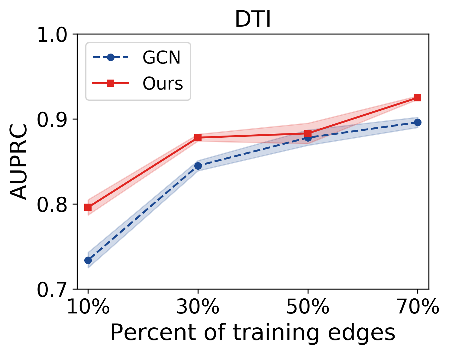
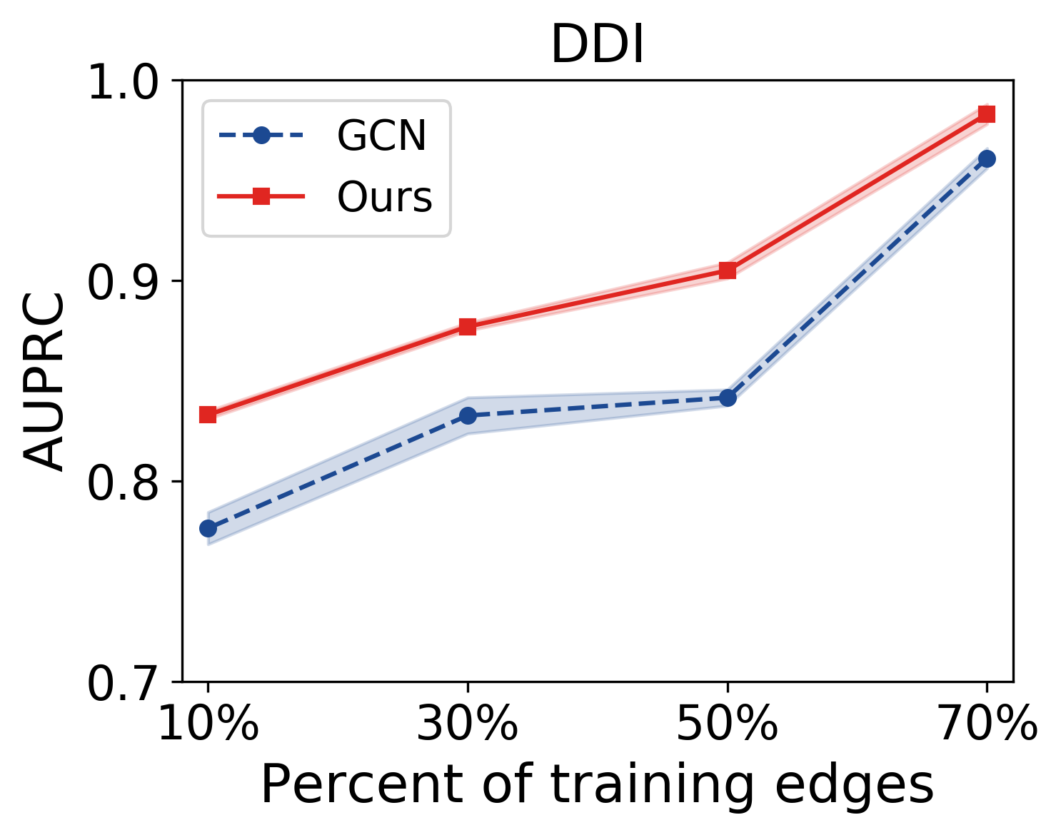
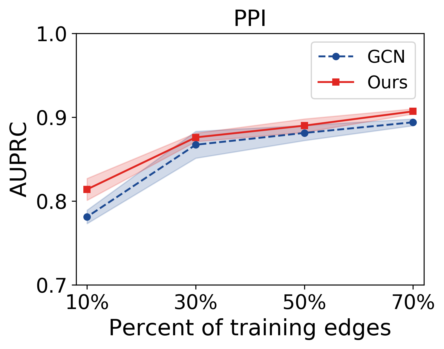
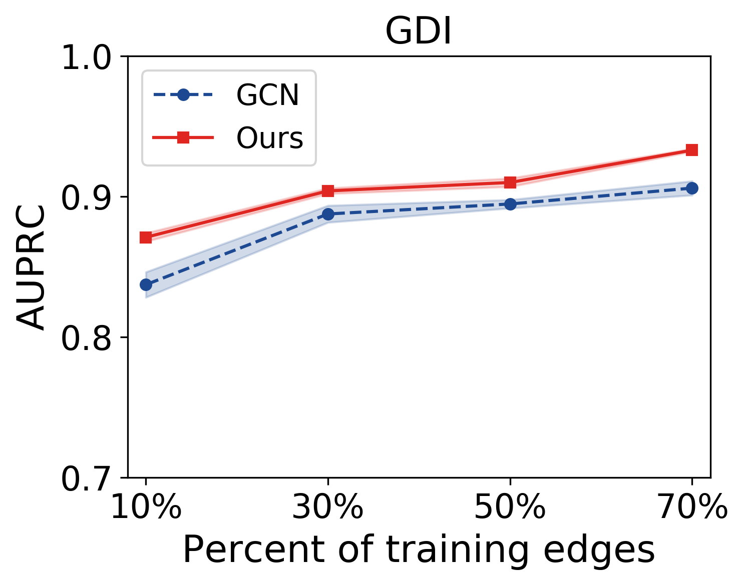
Fig 2: AUPRC comparison for our method and GCNs when trained with different fractions of training edges. (a) DTI (b) DDI (c) PPI and (d) GDI.

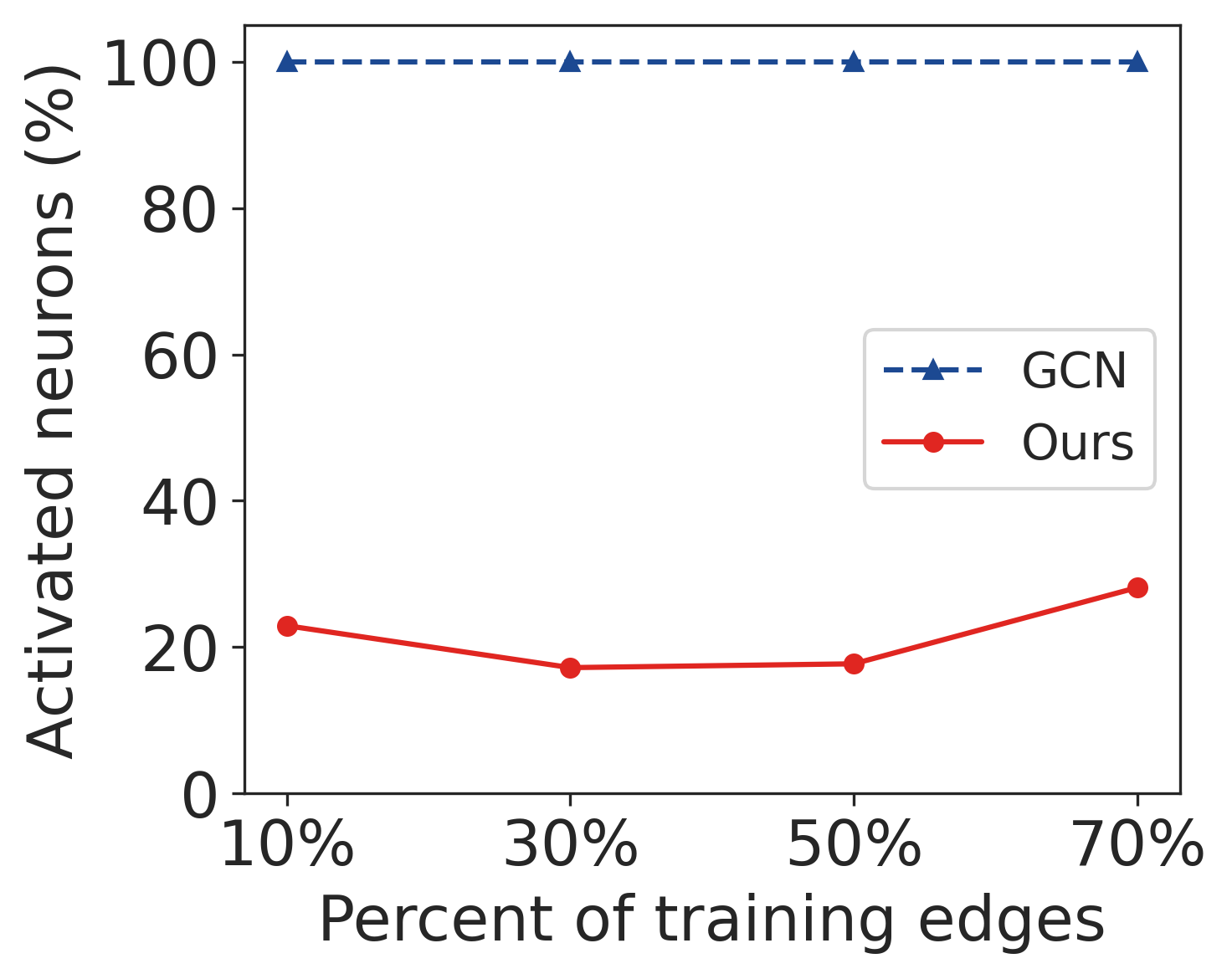
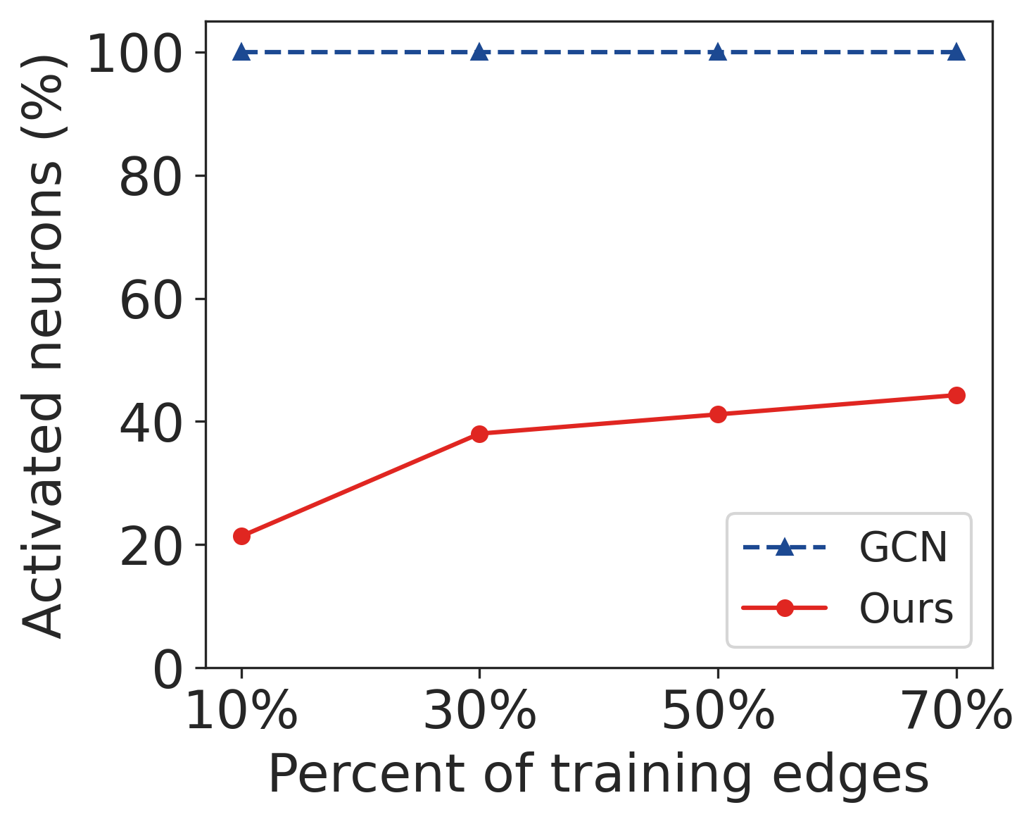
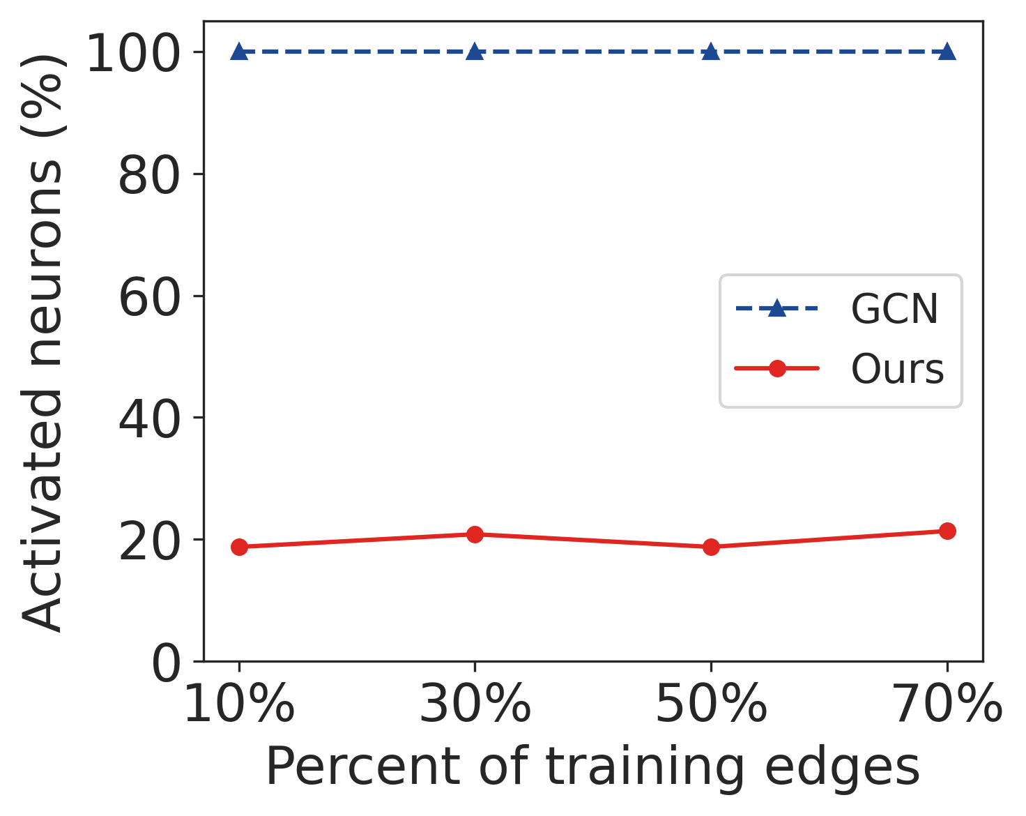
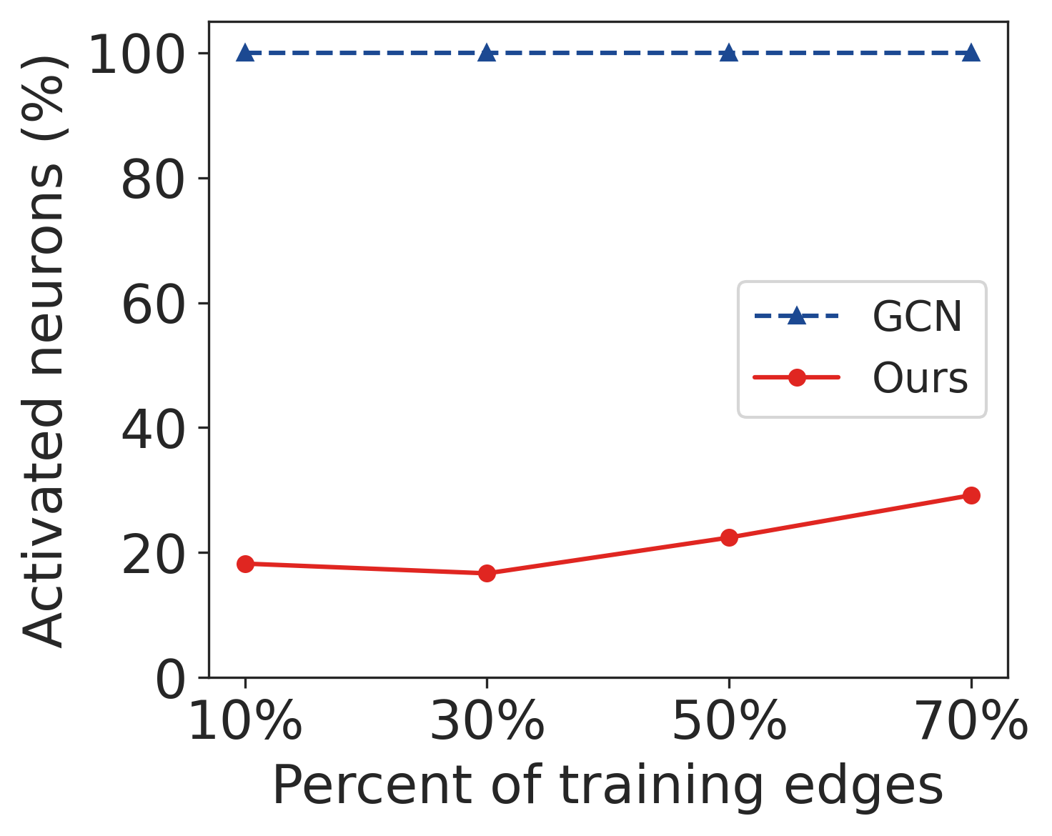
Fig 3: Comparison of activated neurons for our method and GCNs when trained with different number of training interactions. (a) DTI (b) DDI (c) PPI and (d) GDI.

Figure 2 shows that our proposed method is more robust compared to the alternative method. For all datasets, our model’s performance increases with an increase in the number of training interactions. The inference of appropriate depth and their neuron activations enables our model to achieve better performance across all interaction dataset with varying sparsity.

In addition, our proposed method infers an appropriate structure for an encoder for biomedical interaction prediction. Figure 3 shows that the neural network structure dynamically evolves for the DTI prediction task with an increase in percentages of interactions, as our method activates more neurons in the inferred hidden layers. We observe similar behavior for all datasets.

Effect of truncation level $K$

We next investigate if the performance of the model with a predetermined graph convolutional encoder depends on the depth ($L$) of the encoder. Furthermore, we also evaluate the effect of the truncation level $K$ on our model’s performance.

For this experiment, we train predetermined encoder with different depths $L$ over the range $L\in\{1,5,10,15,20\}$. Similarly, we train our proposed framework with truncation level $K$ over the same range $K\in\{1,5,10,15,20\}$. For both methods, we set the maximum number of neurons $M$ in each hidden layer in the encoder to 64. When $L=M=1$, our method has an underfitting problem due to limited model capacity, although our method achieves better performance (Figure 4). When the truncation level $K$ becomes sufficiently large $(K\geq 5)$, the performance of our model does not depend on $K$. Our method essentially works as the Bayesian model selection over the encoder depth which is consistent with the Theorem in [17].

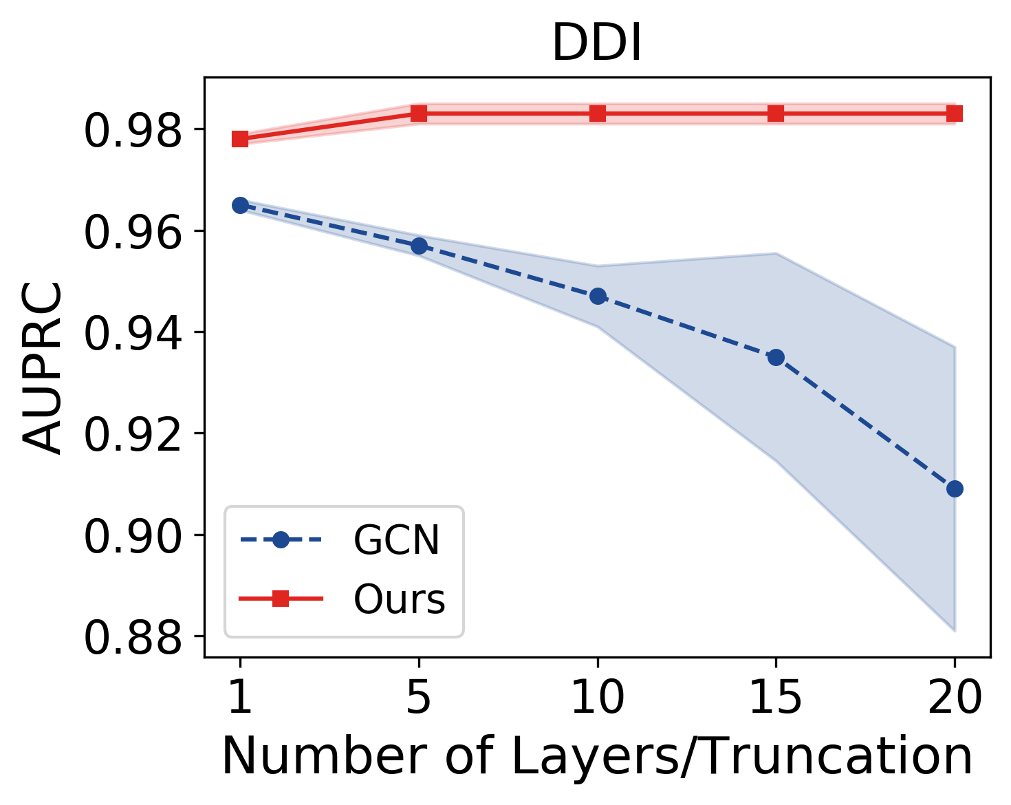
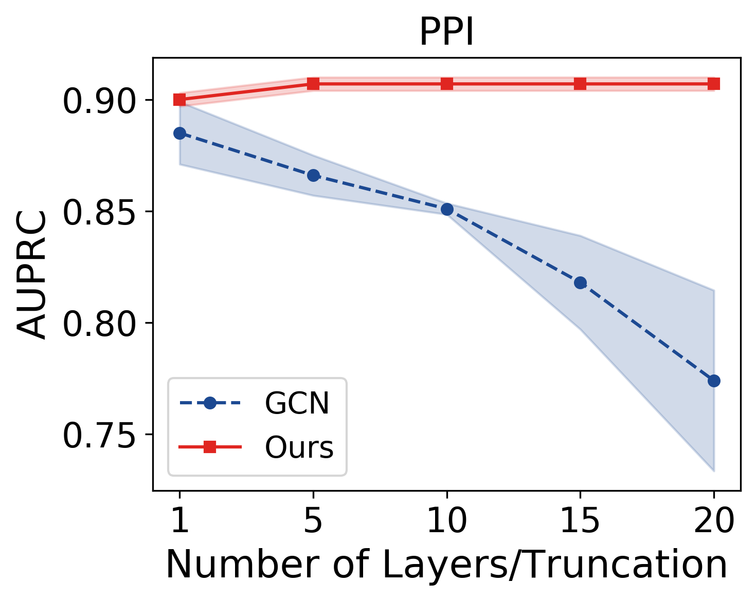
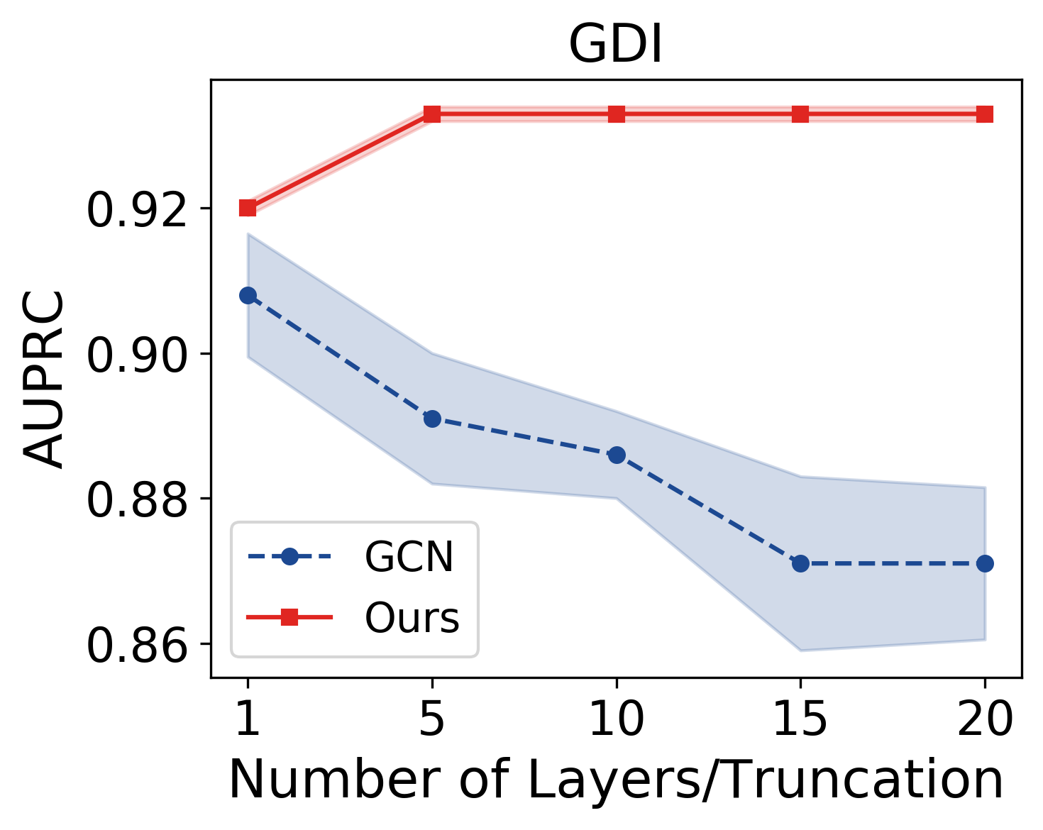
Fig 4: AUPRC comparison for our method with different truncation and GCNs with different number of layers. (a) DTI (b) DDI (c) PPI and (d) GDI.

In contrast, the performance of the GC encoder depends on the depth to a great extent. Figure 4 shows that the GC encoder with predetermined depth suffers from an overfitting problem with the increase in the depth of the encoder. Shallow models with a single hidden layer perform better compared to deeper counterparts. The result in Figure 4 suggests that our method is quite robust to overfitting by jointly inferring the encoder depth and their neuron activations. In addition, our method balances the encoder depth and their network activations to achieve better performances.

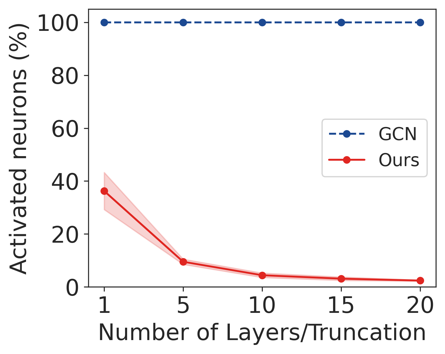
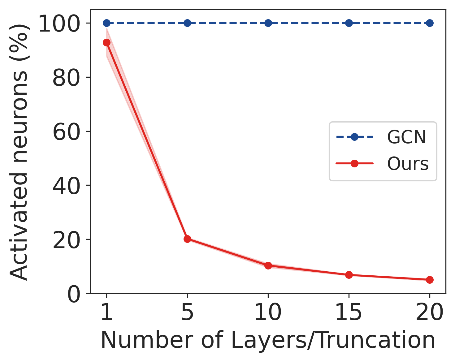
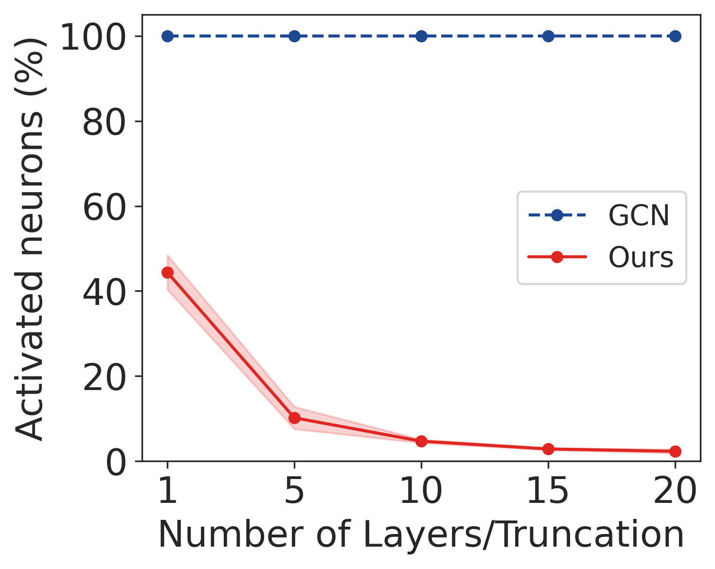
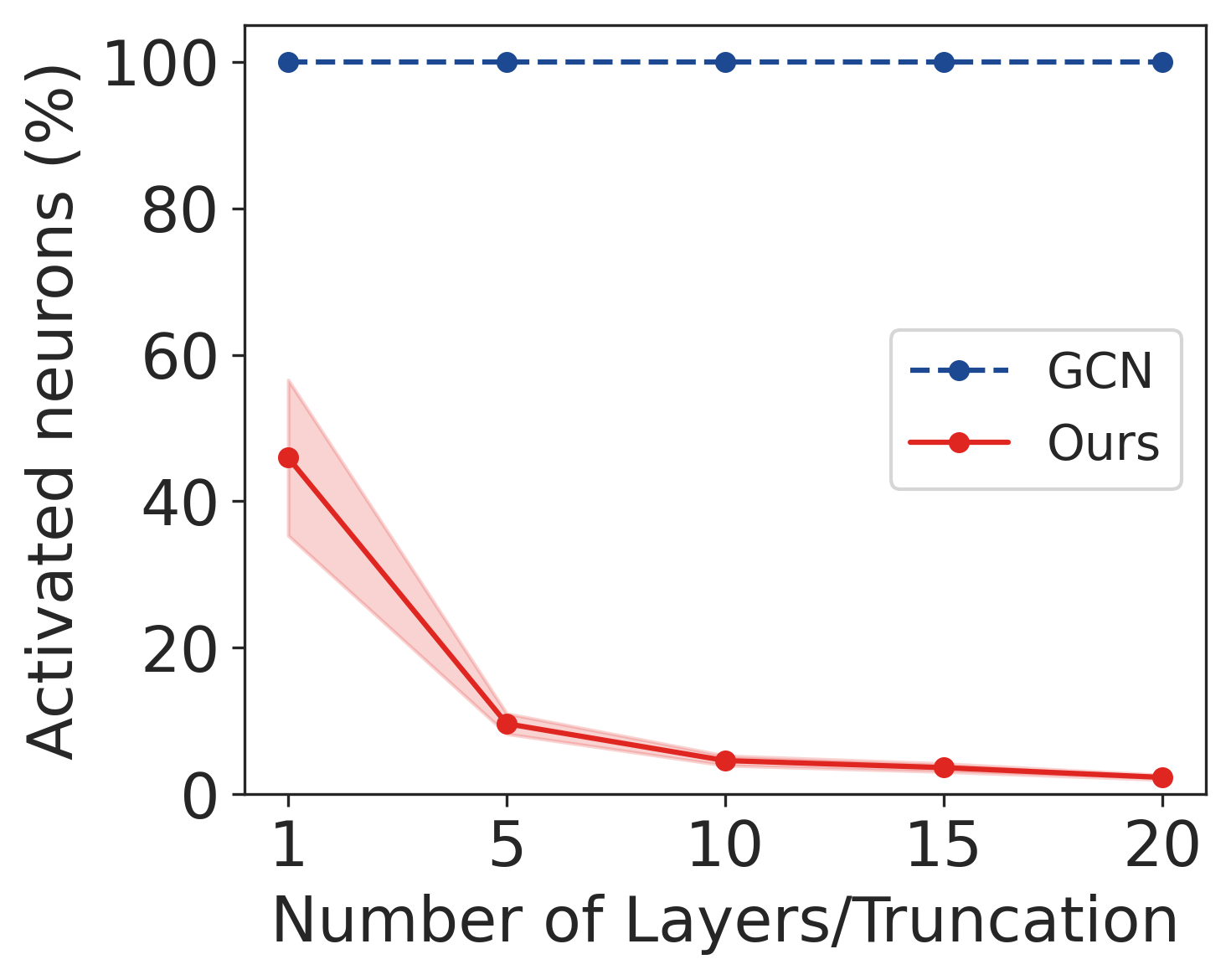
Fig 5: Comparison of activated neurons for our method and GCNs when trained with different truncation $K$ or depth $L$. (a) DTI (b) DDI (c) PPI and (d) GDI.

Furthermore, Figure 5 shows the comparison of the percentage of activated neurons with respect to truncation $K$ or depth $L$. For GCN models with a predetermined encoder structure, all neurons are activated and thus face an overfitting problem. On the contrary, our proposed method regularizes neuron activations and only activates a relatively small number of neurons. With the settings $K=20$, our model activates only 5% neurons.

Analysis of computational efficiency

We further investigate the running time and model size for our method and predetermined GC-based encoder. During training, the predetermined GC-based encoder uses the same network structure over the epochs whereas our proposed inference framework samples different network structures for each forward pass. Figure 6 summarizes the training and testing time for our inference framework and GC-based encoder. Our inference framework takes comparable time to train the model that infers appropriate network structure and also achieves superior performance compared to the predetermined GC-based encoder. With the increase in depth for the predetermined GC-based encoder, the training time and test time increase. On the contrary, our inference framework is robust to larger truncation.

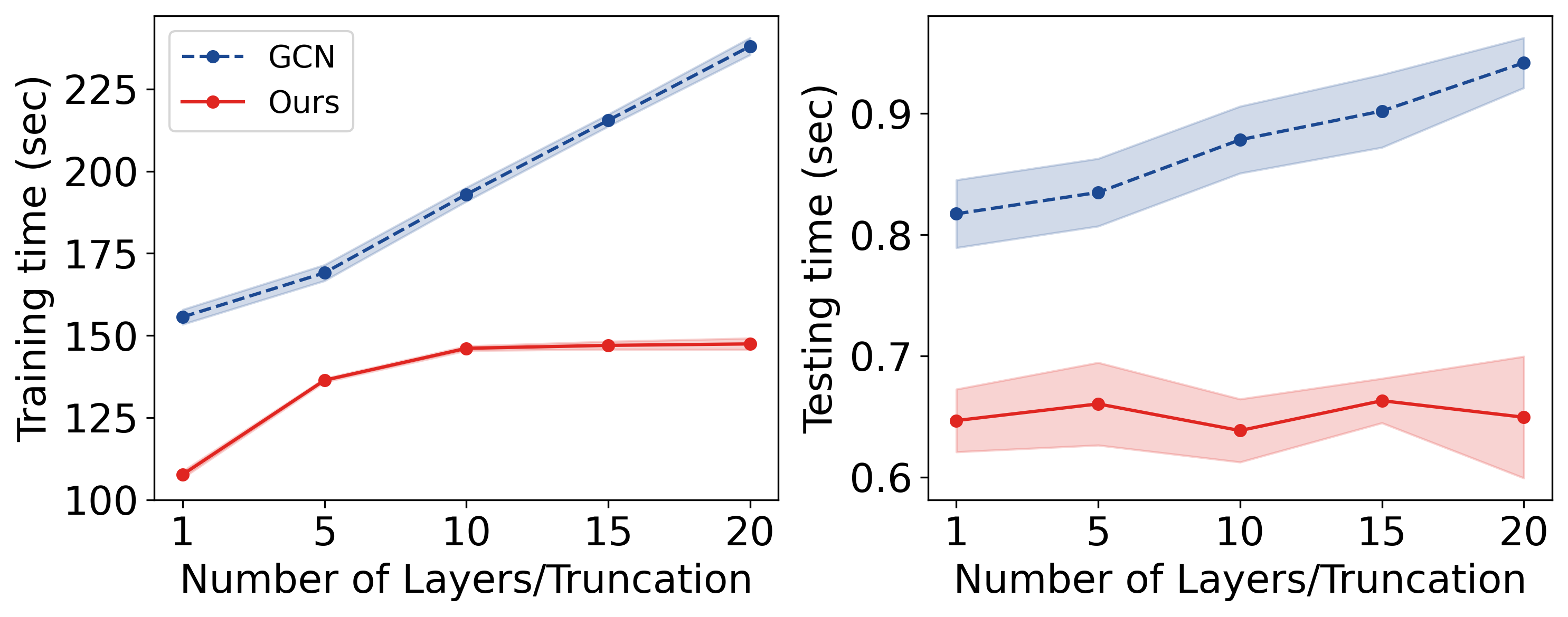
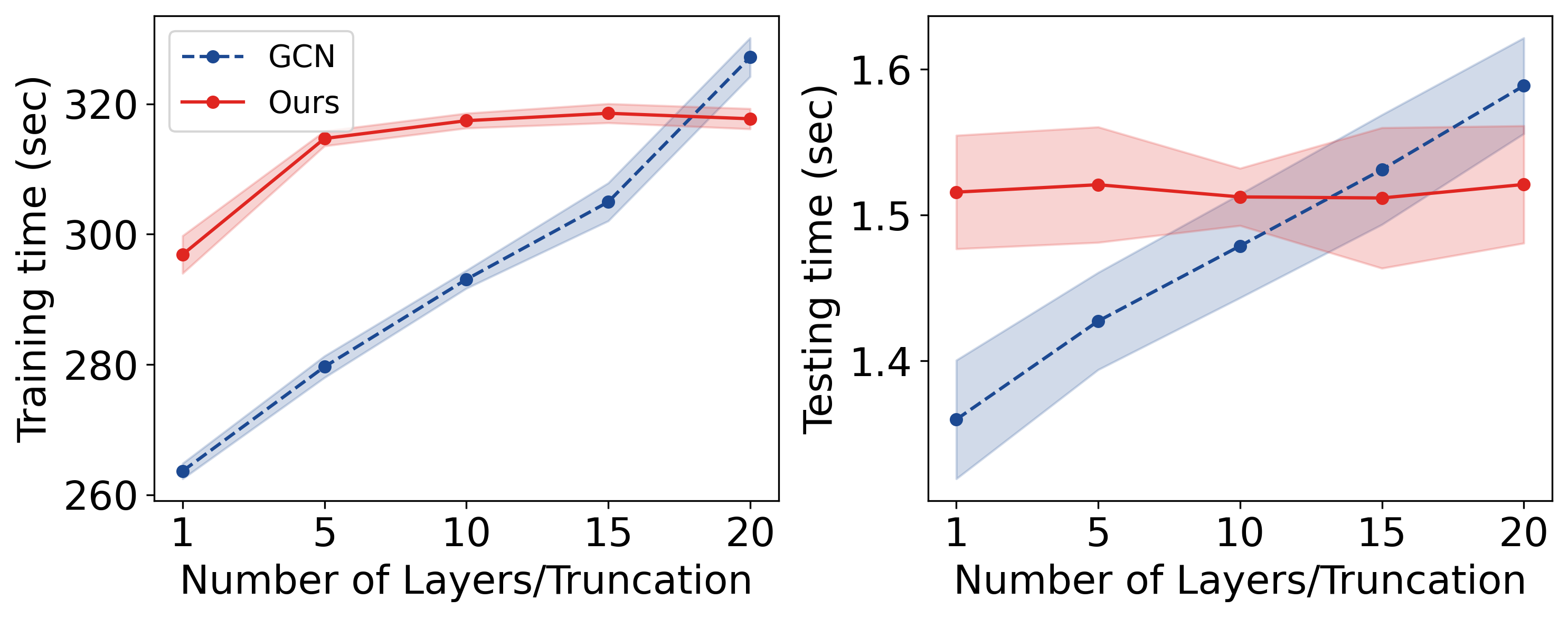
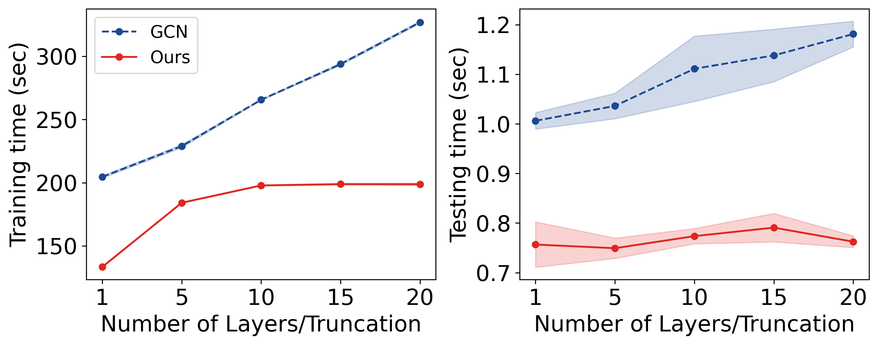
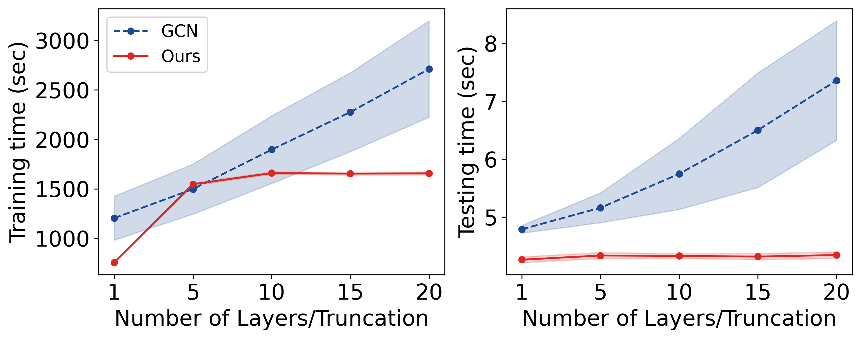
Fig 6: Training and test time comparison of our method with GCNs when trained with different number of layers. (a) DTI (b) DDI (c) PPI and (d) GDI.

Furthermore, we compare the number of parameters for our inference framework and GC-based encoder. For the GC-based encoder, the number of parameters increases with an increase in depth and thus takes more time during the training and testing phase. In contrast, our inference framework does not depend on truncation (Figure 4) and thus the number of parameters is stable across different truncation levels.

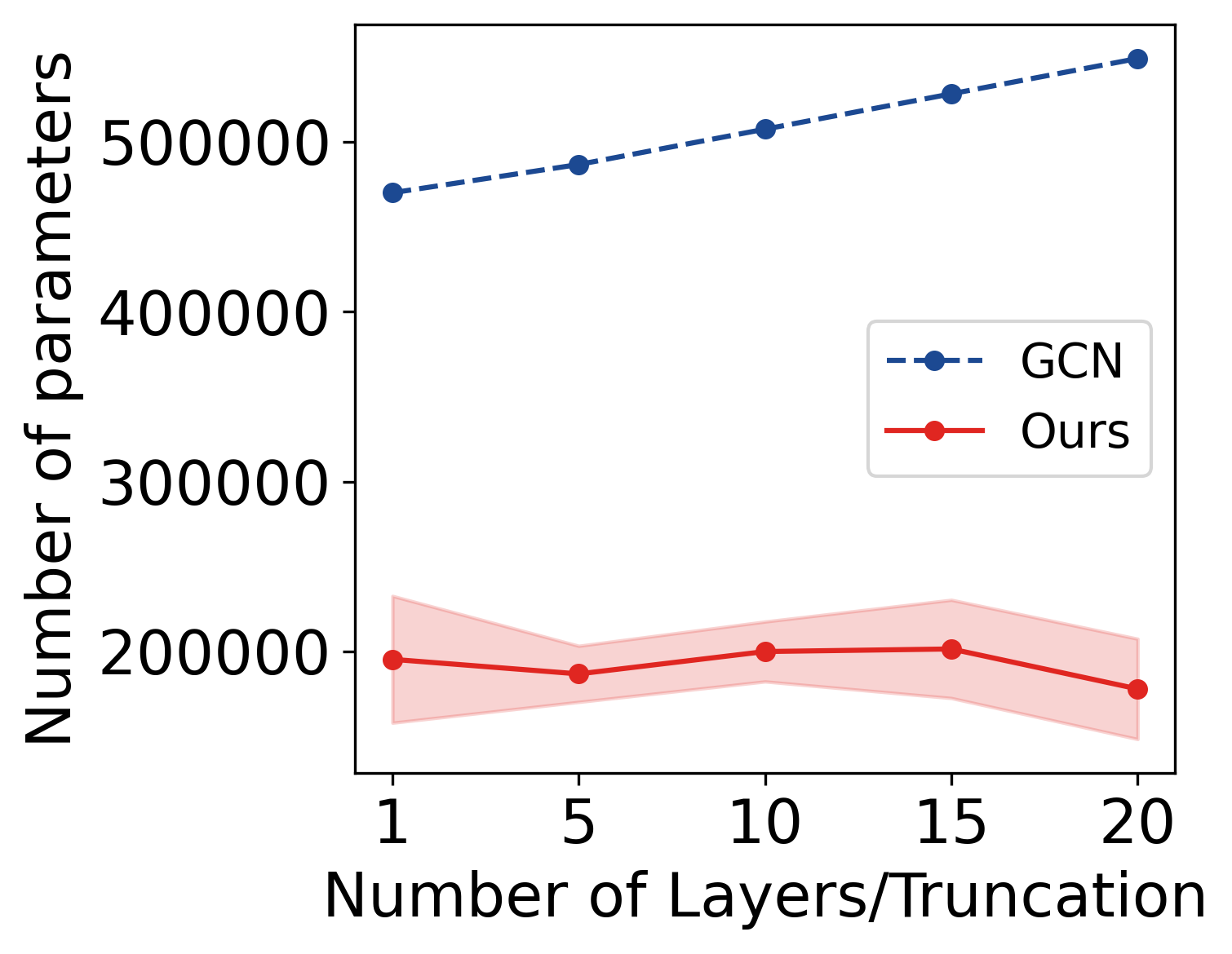
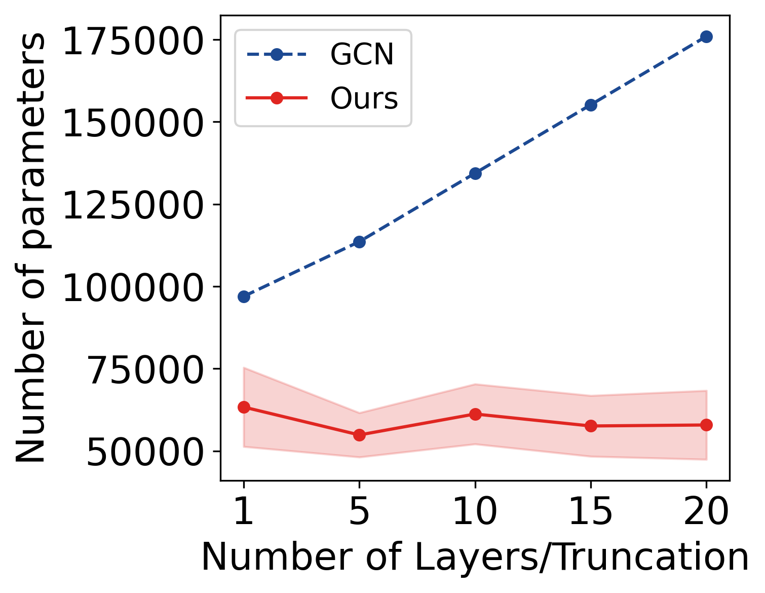
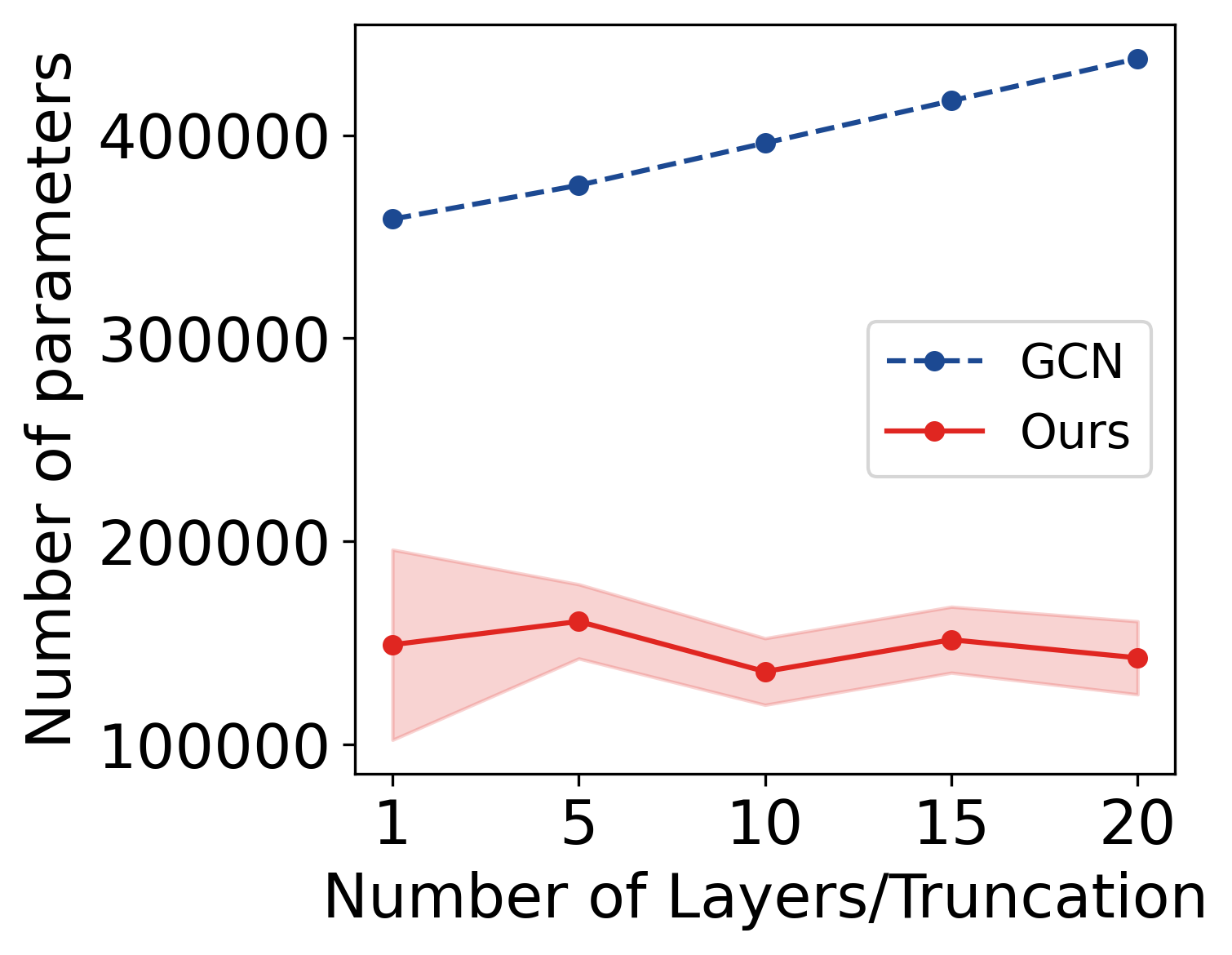
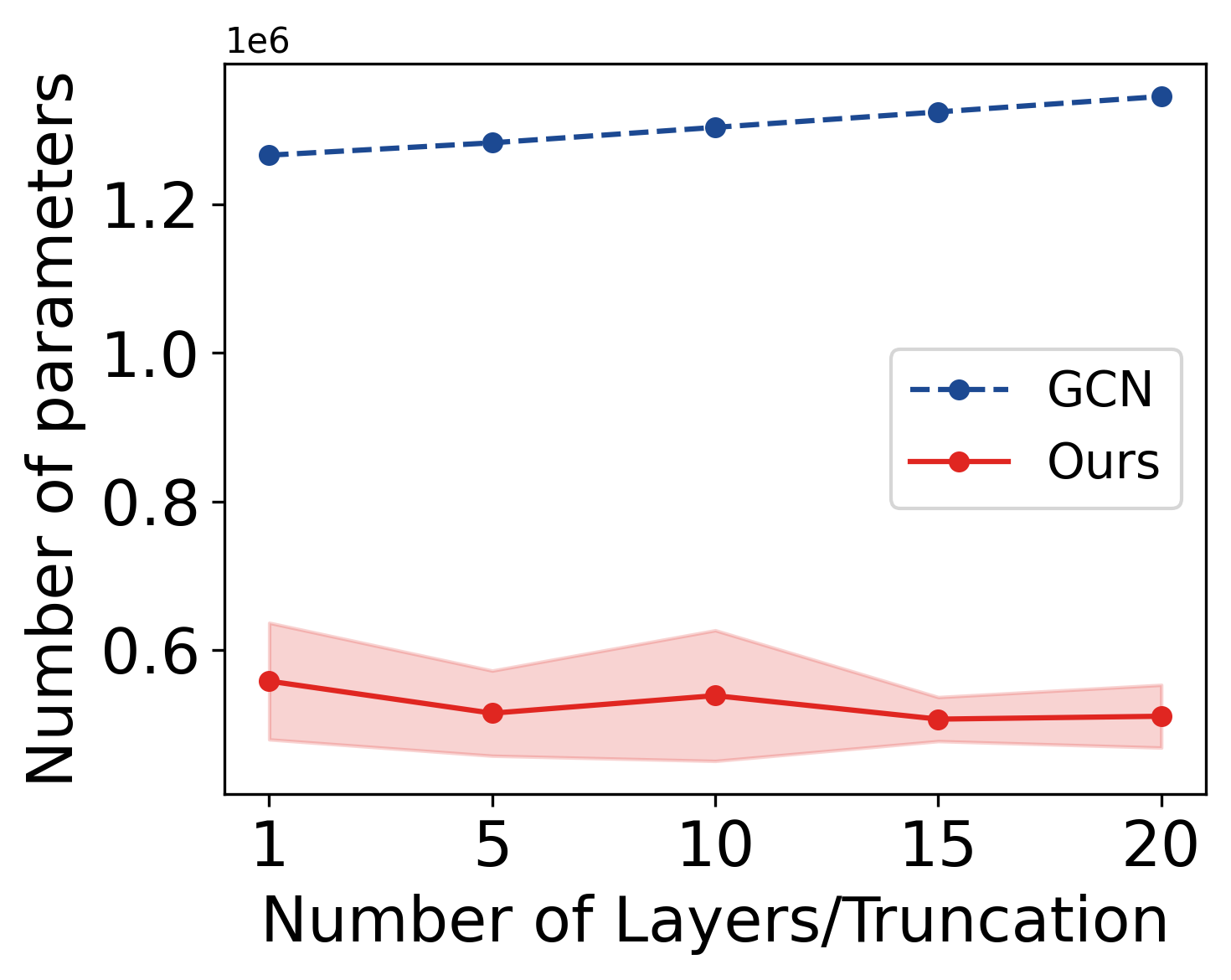
Fig 7: Comparison of parameters of the model trained with different number of layers/truncation. (a) DTI (b) DDI (c) PPI and (d) GDI.

Conclusion

In this paper, we present an inference framework to infer the structure of graph convolution-based encoder. The experiments on GC-based encoder for biomedical interaction prediction show that our method achieves accurate and calibrated predictions by balancing the depth of encoder and neuron activations. We further demonstrate that our inference framework enables the structure of the encoder to dynamically evolve to accommodate the incrementally available number of interactions. Our inference framework infers a compact network structure of encoder with a relatively smaller number of parameters.

References

- 1. Cowen L, Ideker T, Raphael BJ, Sharan R. Network propagation: a universal amplifier of genetic associations. Nature Reviews Genetics. 2017;18(9):551.
- 2. Luck K, Kim DK, Lambourne L, Spirohn K, Begg BE, Bian W, et al. A reference map of the human binary protein interactome. Nature. 2020;580(7803):402–408.
- 3. Zitnik M, Agrawal M, Leskovec J. Modeling polypharmacy side effects with graph convolutional networks. Bioinformatics. 2018;34(13):i457–i466.
- 4. Luo Y, Zhao X, Zhou J, Yang J, Zhang Y, Kuang W, et al. A network integration approach for drug-target interaction prediction and computational drug repositioning from heterogeneous information. Nature communications. 2017;8(1).
- 5. Agrawal M, Zitnik M, Leskovec J, et al. Large-scale analysis of disease pathways in the human interactome. In: PSB. World Scientific; 2018. p. 111–122.
- 6. Kovács IA, Luck K, Spirohn K, Wang Y, Pollis C, Schlabach S, et al. Network-based prediction of protein interactions. Nature communications. 2019;10(1):1–8.
- 7. Perozzi B, Al-Rfou R, Skiena S. Deepwalk: Online learning of social representations. In: Proceedings of the 20th ACM SIGKDD international conference on Knowledge discovery and data mining; 2014. p. 701–710.
- 8. Grover A, Leskovec J. node2vec: Scalable feature learning for networks. In: Proceedings of the 22nd ACM SIGKDD international conference on Knowledge discovery and data mining; 2016. p. 855–864.
- 9. Qiu J, Tang J, Ma H, Dong Y, Wang K, Tang J. DeepInf: Social Influence Prediction with Deep Learning. In: Proceedings of the 24th ACM SIGKDD International Conference on Knowledge Discovery & Data Mining; 2018. p. 2110–2119.
- 10. Ying R, He R, Chen K, Eksombatchai P, Hamilton WL, Leskovec J. Graph Convolutional Neural Networks for Web-Scale Recommender Systems. In: Proceedings of the 24th ACM SIGKDD International Conference on Knowledge Discovery & Data Mining; 2018. p. 974–983.
- 11. Gilmer J, Schoenholz SS, Riley PF, Vinyals O, Dahl GE. Neural message passing for Quantum chemistry. In: Proceedings of the 34th International Conference on Machine Learning-Volume 70; 2017. p. 1263–1272.
- 12. Kipf TN, Welling M. Variational graph auto-encoders. arXiv preprint arXiv:161107308. 2016;.
- 13. Huang K, Xiao C, Glass LM, Zitnik M, Sun J. SkipGNN: predicting molecular interactions with skip-graph networks. Scientific reports. 2020;10(1):1–16.
- 14. KC K, Li R, Cui F, Haake A. Predicting Biomedical Interactions with Higher-Order Graph Convolutional Networks. IEEE/ACM Transactions on Computational Biology and Bioinformatics. 2021;.
- 15. Kipf TN, Welling M. Semi-supervised classification with graph convolutional networks. In: International Conference on Learning Representations; 2017.
- 16. Veličković P, Cucurull G, Casanova A, Romero A, Lio P, Bengio Y. Graph attention networks. In: International Conference on Learning Representations; 2018.
- 17. KC K, Li R, Gilany M. Joint Inference for Neural Network Depth and Dropout Regularization. In: Thirty-Fifth Conference on Neural Information Processing Systems; 2021.Available from: https://openreview.net/forum?id=S5LLQZ-yUP.
- 18. Hamilton WL, Ying R, Leskovec J. Representation learning on graphs: Methods and applications. IEEE Data Engineering Bulletin. 2017;.
- 19. Paisley J, Zaas A, Woods CW, Ginsburg GS, Carin L. A Stick-Breaking Construction of the Beta Process. In: Proc. of the 27th International Conference on Machine Learning (ICML). JMLR. org; 2010. p. 2902–2911.
- 20. Broderick T, Jordan MI, Pitman J. Beta Processes, Stick-Breaking and Power Laws. Bayesian Analysis. 2012;7(2):439–476. doi:10.1214/12-ba715.
- 21. Hoffman MD, Blei DM, Wang C, Paisley J. Stochastic Variational Inference. The Journal of Machine Learning Research. 2013;14(1):1303–1347.
- 22. Hoffman M, Blei D. Stochastic Structured Variational Inference. In: Proc. of the Artificial Intelligence and Statistics (AISTATS); 2015. p. 361–369.
- 23. Brier GW, et al. Verification of forecasts expressed in terms of probability. Monthly weather review. 1950;78(1):1–3.