Self-Supervised Learning based on Heat Equation

Abstract

This paper presents a new perspective of self-supervised learning based on extending heat equation into high dimensional feature space. In particular, we remove time dependence by steady-state condition, and extend the remaining 2D Laplacian from $x$–$y$ isotropic to linear correlated. Furthermore, we simplify it by splitting $x$ and $y$ axes as two first-order linear differential equations. Such simplification explicitly models the spatial invariance along horizontal and vertical directions separately, supporting prediction across image blocks. This introduces a very simple masked image modeling (MIM) method, named QB-Heat.

QB-Heat leaves a single block with size of quarter image unmasked and extrapolates other three masked quarters linearly. It brings MIM to CNNs without bells and whistles, and even works well for pre-training light-weight networks that are suitable for both image classification and object detection without fine-tuning. Compared with MoCo-v2 on pre-training a Mobile-Former with 5.8M parameters and 285M FLOPs, QB-Heat is on par in linear probing on ImageNet, but clearly outperforms in non-linear probing that adds a transformer block before linear classifier (65.6% vs. 52.9%). When transferring to object detection with frozen backbone, QB-Heat outperforms MoCo-v2 and supervised pre-training on ImageNet by 7.9 and 4.5 AP respectively.

This work provides an insightful hypothesis on the invariance within visual representation over different shapes and textures: the linear relationship between horizontal and vertical derivatives. The code will be publicly released.

1 Introduction

Recent work in class activation maps (CAM) [50] shows that convolutional neural networks (CNNs) followed by global average pooling is able to learn categorical heatmap (see Fig. 1) from image level supervision, which is similar to physical heat diffusion governed by heat equation as:

$$\textbf{Heat Equation:}\;\;\;\;\;\;\;\frac{\partial u}{\partial t}=\frac{\partial^{2}u}{\partial x^{2}}+\frac{\partial^{2}u}{\partial y^{2}},$$

where the change of temperature $u$ over time $t$ is related to the change over 2D space $x$, $y$. This motivates us to use heat equation instead of class labels to guide representation learning, thus providing a new perspective of self-supervised learning.

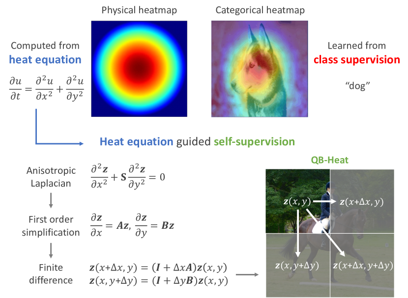
Figure 1: Overview of heat equation guided self-supervised learning. Motivated by the connection between the physical heatmap computed from heat equation and the categorical heatmap (e.g. dog) learned from supervised learning, we leverage heat equation to shift the learning from supervised to self-supervised. By simplifying heat equation into first order linear differential equations followed by finite difference approximation, we develop a simple masked image modeling method (named QB-Heat) that encodes a single unmasked quarter-block to predict other quarters via linear prediction. Best viewed in color.

To achieve this, we extend heat equation from measurable scalar (i.e. temperature $u$) to latent vector (i.e. feature vector $\bm{z}$ with $C$ channels). Then we add steady-state condition $\frac{\partial\bm{z}}{\partial t}=0$ to remove time dependence, and extend 2D isotropic Laplacian into linearly correlated as follows:

$$\textbf{Anisotropic Laplacian}\;\;\;\;\;\;\frac{\partial^{2}\bm{z}}{\partial x^{2}}+\bm{S}\frac{\partial^{2}\bm{z}}{\partial y^{2}}=0,$$

where $\bm{z}$ is feature map with $C$ channels, i.e. $\bm{z}(x,y)\in\mathbb{R}^{C}$, and $\bm{S}$ is a $C$$\times$$C$ matrix. Here $\bm{S}$ plays two roles: (a) handling nonequivalent change over horizontal and vertical directions, and (b) encoding invariant relationship between the second order of derivatives along $x$ and $y$ axes in the latent representation space. Furthermore, we decouple this spatial invariance along $x$ and $y$ axes separately to simplify the anisotropic Laplacian into two first order linear differential equations as follows:

$$\textbf{First order linear:}\;\;\;\;\frac{\partial\bm{z}}{\partial x}=\bm{A}\bm{z},\;\;\frac{\partial\bm{z}}{\partial y}=\bm{B}\bm{z},$$

where $\bm{A}$ and $\bm{B}$ are invertible matrices with size $C$$\times$$C$ and $\bm{S}$$=$$-\bm{A}^{2}(\bm{B}^{2})^{-1}$.

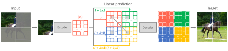
Figure 2: QB-Heat architecture. An encoder is applied on a single unmasked quarter-block to extract feature map $\{\bm{z}_{i}\}$, leaving other three quarters masked. The prediction is performed between corresponding positions from unmasked to masked quarters through linear projection. A projection matrix is shared over all positions within each quarter, but three masked quarters have different projection matrices, i.e. $\bm{I}$$+$$\Delta x\bm{A}$, $\bm{I}$$+$$\Delta y\bm{B}$, and $(\bm{I}$$+$$\Delta x\bm{A})(\bm{I}$$+$$\Delta y\bm{B})$. Then a small decoder is used to reconstruct the original image in pixels. The self-prediction is based on the finite difference approximation, e.g. $\bm{z}(x$$+$$\Delta x,y)$$=$$(\bm{I}$$+$$\Delta x\bm{A})\bm{z}(x,y)$, where the spatial offsets are half width/height of the image, i.e. $\Delta x$$=$$W/2$, $\Delta y$$=$$H/2$. Best viewed in color.

This simplification not only has nice properties, like holding linear relationship for any order derivatives between $x$ and $y$ as $\frac{\partial^{n}\bm{z}}{\partial x^{n}}$$=$$\bm{A}^{n}(\bm{B}^{m})^{-1}\frac{\partial^{m}\bm{z}}{\partial y^{m}}$, but also allows horizontal and vertical prediction based on its finite difference approximation as follows:

$$\textbf{Finite}\;\;\;\;\;\;\;\;\bm{z}(x+\Delta x,y)-\bm{z}(x,y) =\Delta x\bm{A}\bm{z}(x,y)$$

$$\textbf{difference}\;\;\;\;\bm{z}(x,y+\Delta y)-\bm{z}(x,y) =\Delta y\bm{B}\bm{z}(x,y).$$

This gives rise to a new masked image modeling method. Specifically, only a single quarter-block is unmasked to encode $\bm{z}(x,y)$, which is used to predict other three masked quarters $\bm{z}(x$$+$$\Delta x,y)$, $\bm{z}(x,y$$+$$\Delta y)$, $\bm{z}(x$$+$$\Delta x,y$$+$$\Delta y)$ via linear prediction (see Fig. 1, 2). The learning target includes encoder $\bm{z}$ and matrices $\bm{A}$, $\bm{B}$. We name this Quarter-Block prediction guided by Heat equation as QB-Heat. Compared to popular MAE [25], it has four differences:

• more regular masking (a single unmasked quarter).

• simpler linear prediction.

• enabling masked image modeling for efficient CNN based architectures without bells and whistles.

• modeling spatial invariance explicitly in representation space via learnable matrices $\bm{A}$ and $\bm{B}$.

We also present an evaluation protocol, decoder probing, in which the frozen pre-trained encoder (without fine-tuning) is evaluated over two tasks (image classification and object detection) with different decoders. Decoder probing includes widely used linear probing, but extends from it by adding non-linear decoders. It directly evaluates encoders as they are, complementary to fine-tuning that evaluates pre-trained models indirectly as initial weights.

QB-Heat brings masked image modeling to CNN based architectures, even for pre-training light-weight networks. Moreover, the pre-trained encoders are suitable for both image classification and object detection without fine-tuning. For instance, when pre-training a Mobile-Former [12] with 5.8M parameters and 285M FLOPs, QB-Heat is on par with MoCo-v2 [9] in linear probing on ImageNet, but outperforms by a clear margin (65.6% vs. 52.9%) in non-linear decoder probing that adds a transformer block before the linear classifier. When transferring to object detection with frozen backbone, QB-Heat outperforms MoCo-v2 and supervised pre-training on ImageNet by 7.9 and 4.5 AP respectively. In addition, we found that fine-tuning QB-Heat pre-trained encoders on ImageNet-1K alone introduces consistent gain on object detection, thus providing strong encoders shared by classification and detection tasks. For example, 82.5% top-1 accuracy on ImageNet and 45.5 AP on COCO detection (using 100 queries in DETR framework) are achieved by sharing a Mobile-Former with 25M parameters and 3.7G FLOPs (similar to ResNet-50 and ViT-S).

The solid performance demonstrates that the simplified heat equation (from anisotropic Laplacian to first order linear differential equations) sheds light on the spatial invariance of visual representation: horizontal and vertical partial derivatives are linearly correlated. We hope this will encourage exploration of principles in visual representations.

2 Related Work

Contrastive methods [4, 24, 44, 47, 26, 10, 6] achieve significant progress recently. They are most applied to Siamese architectures [7, 26, 9, 11] to contrast image similarity and dissimilarity and rely on data augmentation. [10, 23] remove dissimilarity between negative samples by handling collapse carefully. [8, 34] show pre-trained models work well for semi-supervised learning and few-shot transfer.

Information maximization provides another direction to prevent collapse. W-MSE [19] avoids collapse by scattering batch samples to be uniformly distributed on a unit sphere. Barlow Twins [48] decorrelates embedding vectors from two branches by forcing cross-correlation matrix to identity. VICReg [3] borrows decorrelation mechanism from Barlow Twins, but explicitly adds variance-preservation for each variable of two embeddings.

Masked image modeling (MIM) is inspired by the success of BERT [15] and ViT [18] to learn representation by predicting masked region from unmasked counterpart. BEiT [2] and PeCo [16] predict on tokens, MaskFeat [46] predicts on HOG, and MAE [25] reconstructs original pixels. Recent works explore further improvement by combining MIM and contrastive learning [51, 17, 30, 43, 1] or techniques suitable for ConvNets [22, 31, 20]. Different from these works that rely on random masking or ViT, our QB-Heat uses regular masking and simpler linear prediction to enable MIM for efficient CNNs without bells and whistles.

3 Heat Equation in Feature Space

In this section, we discuss in details how to extend heat equation $\frac{\partial u}{\partial t}=\frac{\partial^{2}u}{\partial x^{2}}+\frac{\partial^{2}u}{\partial y^{2}}$ from a uni-dimensional and observed variable (i.e. temperature $u$) into multi-dimensional and latent feature space $\bm{z}$.

Motivation: Motivated by class activation maps (CAM) [50] in which the categorical heatmap is similar to physical heat diffusion (see Fig. 1), we hypothesize that (a) the feature map around a visual object is smooth and governed by heat equation, and (b) the corresponding feature encoder can learn from heat equation alone without any labels. These hypotheses are hard to prove, but instead we show their potential in self-supervised learning. Next, we discuss how to extend heat equation into feature space.

Extending heat equation into linear systems: The extension of heat equation is based on two design guild-lines: (a) the heat diffusions along multiple feature channels are correlated, and (b) the diffusions along horizontal and vertical directions are not equivalent. The former is straightforward as most of neural architectures output highly correlated features. The latter is due to the shape and texture anisotropy in visual objects which determines the heat diffusions along features. This is different with original heat equation which is spatial isotropy on a single channel.

Based on these two guild-lines, we firstly replace temperature $u$ in the original heat equation with feature vector $\bm{z}\in\mathbb{R}^{C}$ and use the steady-state condition $\frac{\partial\bm{z}}{\partial t}=0$ to remove time dependence, resulting in a Laplacian equation $\frac{\partial^{2}\bm{z}}{\partial x^{2}}+\frac{\partial^{2}\bm{z}}{\partial y^{2}}=0$. Then, we extend Laplacian from spatial isotropy to anisotropy by adding a coefficient matrix $\bm{S}$ with size $C\times C$ as $\frac{\partial^{2}\bm{z}}{\partial x^{2}}+\bm{S}\frac{\partial^{2}\bm{z}}{\partial y^{2}}=0$. To allow self-prediction along horizontal and vertical directions, we decouple $x$ and $y$ axes in Laplacian into two first-order linear differential equations as:

$$\frac{\partial\bm{z}}{\partial x}=\bm{A}\bm{z},\;\;\frac{\partial\bm{z}}{\partial y}=\bm{B}\bm{z},\;\;\;\;\bm{S}=-\bm{A}^{2}(\bm{B}^{2})^{-1},$$ (1)

where $\bm{A}$ and $\bm{B}$ are two $C\times C$ matrices. Note that $\bm{A}$ and $\bm{B}$ are commuting matrices $\bm{AB}=\bm{BA}$ if $\bm{z}(x,y)$ has continuous second partial derivatives based on the Clairaut’s theorem ($\frac{\partial^{2}\bm{z}}{\partial x\partial y}=\bm{BAz}=\bm{ABz}=\frac{\partial^{2}\bm{z}}{\partial y\partial x}$). Here, we assume $\bm{A}$ and $\bm{B}$ are invertible matrices to achieve $\bm{S}$.

Properties: The first-order simplification above is a special case of Laplacian that has nice properties as follows.

Property 1: linear relationship holds for any order derivatives between horizontal and vertical directions as:

$$\frac{\partial^{n}\bm{z}}{\partial x^{n}}=\bm{A}^{n}\bm{z},\;\;\;\;\frac{\partial^{m}\bm{z}}{\partial y^{m}}=\bm{B}^{m}\bm{z},$$

$$\frac{\partial^{n}\bm{z}}{\partial x^{n}}-\bm{A}^{n}(\bm{B}^{m})^{-1}\frac{\partial^{m}\bm{z}}{\partial y^{m}}=0.$$ (2)

Property 2 – solution has exponential format as:

$$\bm{z}(x,y)=e^{\bm{A}x}e^{\bm{B}y}\bm{z}(0,0),$$ (3)

where the exponential matrix $e^{\bm{A}x}$ is defined by Taylor expansion $e^{\bm{A}x}$$=$$\sum_{n=0}^{\infty}(\bm{A}x)^{n}/n!$, and $\bm{z}(0,0)$ is the initial vector. Since $\bm{A}$ and $\bm{B}$ are commuting matrices (i.e. $\bm{AB}=\bm{BA}$), they share eigenvectors (denoted as $\bm{v}_{i}$) when $\bm{A}$ has distinct eigenvalues. Thus, Eq. 3 can be written as:

$$\bm{z}(x,y)=\sum_{i=1}^{C}c_{i}e^{\lambda_{i}x+\pi_{i}y}\bm{v}_{i},$$ (4)

where $\{\lambda_{i}\}$ and $\{\pi_{i}\}$ are eigenvalues for $\bm{A}$ and $\bm{B}$, respectively. The coefficient $c_{i}$ is determined by initial vector $\bm{z}(0,0)$ such that $\sum_{i}c_{i}\bm{v}_{i}=\bm{z}(0,0)$.

From continuous to discrete: In practice, we approximate continuous coordinates ($x$, $y$) by using discrete measure over $H\times W$ locations, converting Eq. 1 to difference over small segment ($\Delta x$ or $\Delta y$) as follows:

$$\bm{z}(x+\Delta x,y)-\bm{z}(x,y) =\Delta x\bm{A}\bm{z}(x,y)$$

$$\bm{z}(x,y+\Delta y)-\bm{z}(x,y) =\Delta y\bm{B}\bm{z}(x,y).$$ (5)

Collapse solution: Both continuous Eq. 1 and discrete Eq. 5 have a collapse solution, i.e. feature map has constant value $\bm{z}(x,y)=c$, and $\bm{A}$ and $\bm{B}$ are zero matrices. Inspired by LeCun’s seminal paper [32] that discusses multiple ways to handle collapse, we propose a new masked image modeling guided by Eq. 5 to handle collapse. In particular, we mask out $(x$$+$$\Delta x,y)$ and $(x,y$$+$$\Delta y)$ and predict their features from unmasked $\bm{z}(x,y)$ using linear projection in Eq. 5. This new self-supervised pre-training based on linear differential equations is named QB-Heat, which will be discussed in details next.

4 QB-Heat

We now introduce Quarter-Block prediction guided by Heat equation (QB-Heat), that performs self-prediction based on Eq. 5. It not only prevents collapse but also enables masked image modeling for CNN based architectures.

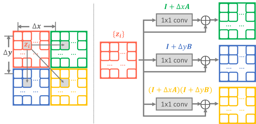
Figure 3: Implementation of translational linear prediction. The feature map extracted from the unmasked top-left quarter of the input image is used to predict feature maps for other three masked quarters using 1$\times$1 convolution. Best viewed in color.

4.1 Linear Prediction based on Quarter Masking

QB-Heat only uses a single unmasked block to extrapolate over masked area via linear prediction. This resolves the conflict between random masking and CNN based encoder. The unmasked block has quarter size of the input image (see Fig. 2) and goes through encoder to extract features. Then, linear prediction is performed over three masked quarter-blocks followed by a decoder to reconstruct the original image. The linear prediction is element-wise and can be implemented as 1$\times$1 convolution (see Fig. 3). Each masked quarter-block has its own linear model, which is shared by all elements within the block. QB-Heat has two components to adjust: (a) the position of the unmasked quarter-block, and (b) the number of explicit linear models, which are discussed below.

Position of unmasked quarter-block: The unmasked quarter-block are either at four corners or at the center (see Fig. 4), corresponding to prediction at different translation scales. Placing the unmasked quarter at corner corresponds to a larger prediction offset $\Delta x$$=$$W/2$, $\Delta y$$=$$H/2$, while prediction from the center quarter-block is at a finer scale $\Delta x$$=$$W/4$, $\Delta y$$=$$H/4$ after splitting it into four sub-blocks. Our experiments show that mixing corner and center positions in a batch provides the best performance.

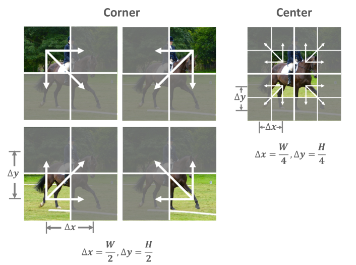
Figure 4: Position of the unmasked quarter-block. The corner position corresponds to prediction over larger translation ($\Delta x$$=$$W/2$, $\Delta y$$=$$H/2$) than the center position ($\Delta x$$=$$W/4$, $\Delta y$$=$$H/4$).

Number of explicit linear models: As shown in Fig. 4, prediction across blocks is performed along 8 directions in total for both corner and center positioning of the unmasked quarter. Two of them (right, down) are included in difference equations ($\bm{A}$, $\bm{B}$ in Eq. 5). The other six can be either derived from $\bm{A}$ and $\bm{B}$ (see Appendix A for details) or modeled explicitly by adding linear models. Fig. 5 shows three variants that have 2, 4 and 8 explicit linear models (solid arrow) respectively. The remaining directions (dash arrow) are derived from explicit models. Experiments show two explicit models work well, demonstrating $\bm{A}$ and $\bm{B}$ effectively encode the feature change.

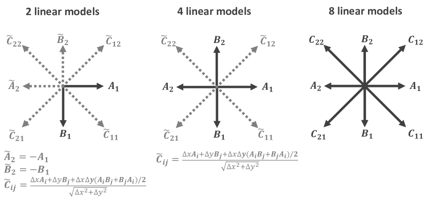
Figure 5: Number of explicit linear models. A solid arrow indicates an explicit linear model, while a dash arrow indicates an implicit model derived from the explicit counterparts.

4.2 Architecture and Implementation

QB-Heat follows masked autoencoder [25] architecture that includes masking, encoder, predictor and decoder.

Masking: QB-Heat has a single unmasked block with quarter size of the input image, which is located at either corners or center (see Fig. 4). This is consistent with MAE in masking ratio (75%), but is applicable for CNN based encoder.

QB-Heat encoder: We use Mobile-Former [12] as encoder, which is a CNN based network (adding 6 global tokens in parallel to MobileNet [39]). To retain more spatial details, we increase the resolution for the last stage from $\frac{1}{32}$ to $\frac{1}{16}$. Three Mobile-Former variants (with 285M, 1.0G, 3.7G FLOPs) are used for evaluation. All of them has 12 blocks and 6 global tokens (see Tab. 8 in Sec. B.1).

QB-Heat predictor: The output features of the unmasked quarter-block are projected to 512 dimensions and followed by linear models (implemented as 1$\times$1 convolution in Fig. 3) to predict for masked blocks. This predictor is only used in pre-training and removed during inference.

QB-Heat decoder: We follow MAE [25] to apply a series of transformer blocks as decoder on both unmasked and masked quarter-blocks. In this paper, we use 6 transformer blocks with dimension 512 in decoder.

4.3 Relation to MAE

QB-Heat differentiates from MAE [25] by explicitly modeling feature derivatives using linear differential equations, enabling more regular masking and simpler prediction to support more efficient CNN based networks.

More regular masking: Different with random unmasked patches in MAE, QB-Heat has a single unmasked quarter-block, suitable for CNNs without bells and whistles. Compared to MAE with regular block-wise masking that achieves 63.9% in linear probing and 82.8% in fine-tuning on ImageNet-1K by using ViT-L with 307M parameters, QB-Heat achieves similar performance (65.1% in linear probing, 82.5% in fine-tuning) more efficiently by using Mobile-Former-3.7G with 35M parameters.

Simpler prediction: In QB-Heat, each masked patch is predicted from a single unmasked patch with translation $\Delta x$ or $\Delta y$ (see Fig. 3) rather than aggregating all unmasked patches in MAE, thus resulting in much lower complexity.

5 Evaluation: Decoder Probing

In this section, we propose a new evaluation protocol for self-supervised pre-training to complement widely used linear probing and fine-tuning. Linear probing is sensitive to feature dimension and misses the opportunity of pursuing non-linear features [25], while fine-tuning indirectly evaluates a pre-trained model as initial weights for downstream tasks. We need a new protocol that (a) can handle both linear and non-linear features, (b) performs direct evaluation without fine-tuning, (c) covers multiple visual tasks. It encourages exploration of pre-training a universal (or task-agnostic) encoder.

Decoder probing provides a solution. It involves multiple tasks such as image classification and object detection. For each task, only the decoder is learnable while the pre-trained encoder (backbone) is frozen. Each task has a set of decoders with different complexities to provide comprehensive evaluation. Below we list decoders used in this paper.

Classification decoders: We use two simple classification decoders: (a) linear decoder (or linear probing) including global average pooling and a linear classifier, and (b) transformer decoder that adds a single transformer block before global pooling (denoted as tran-1). The transformer block is introduced to encourage representative features that are not ready to separate categories linearly yet, but can achieve it by the assistance of a simple decoder.

Detection decoders: We use three detection decoders: two DETR [5] heads and one RetinaNet [36] head. The two DETR heads use Mobile-Former [12] over three scales ($\frac{1}{32}$, $\frac{1}{16}$, $\frac{1}{8}$) with different depths. The shallower one (denoted as MF-Dec-211) has four blocks (two in $\frac{1}{32}$, one in $\frac{1}{16}$, one in $\frac{1}{8}$), while the deeper one (denoted as MF-Dec-522) has nine blocks (five in $\frac{1}{32}$, two in $\frac{1}{16}$, two in $\frac{1}{8}$). Please see Tab. 13 in Sec. B.2 for details.

encoder	madds	param	lin
Mob-v3 [29]†	217M	5.4M	36.3
Eff-b0 [42]†	390M	5.3M	42.2
Eff-b1 [42]†	700M	7.8M	50.7
MF-285M [12]‡	285M	5.8M	51.6

encoder	madds	param	lin
Res-18 [27]†	1.8G	11.7M	52.5
Res-34 [27]†	3.6G	21.8M	57.4
MF-1.0G [12]‡	1.0G	13.5M	60.4

Table 1: Linear probing results of efficient networks pre-trained by MoCo-v2 [9]. “MF” (e.g. MF-285M) refers to Mobile-Former. ^† and ^‡ indicate implementation in [21] and this paper respectively.

position (prediction offset)	lin	tran-1	ft
corner ($\Delta x$$=$$W/2,\Delta y$$=$$H/2$)	64.1	77.9	82.1
center ($\Delta x$$=$$W/4,\Delta y$$=$$H/4$)	64.2	77.9	82.4
corner + center	lightgray65.1	lightgray78.6	lightgray 82.5
(a) Position of the unmasked quarter-block.

#models	lin	tran-1	ft
2	64.8	78.4	82.3
4	65.0	78.5	82.4
8	lightgray65.1	lightgray78.6	lightgray82.5
(b) Number of linear models.

Table 2: QB-Heat ablation experiments with Mobile-Former-3.7G on ImageNet-1K. We report top-1 accuracy (%) of two decoder probings, i.e. linear (lin) and transformer (tran-1), and fine-tuning with transformer decoder (ft). Two properties are observed: (a) multi-scale prediction (corner+center) is better than single scale, and (b) two explicit linear models ($\bm{A}$, $\bm{B}$ in Eq. 5) are good enough. Default settings are marked in gray.

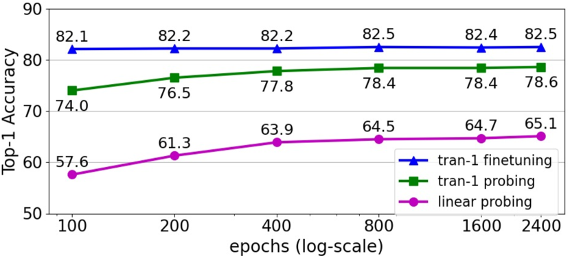
Figure 6: Training schedules. Longer training provides consistent improvement for linear and tran-1 probing, while fine-tuning is not sensitive to training schedule.

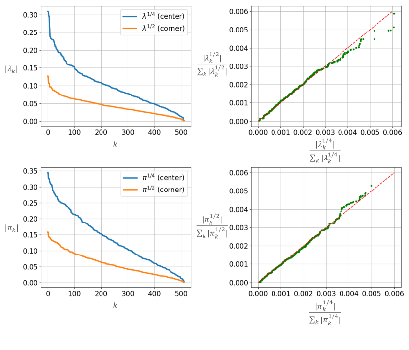
Figure 7: Spectrum of matrices $\bm{A}$ and $\bm{B}$ learned from QB-Heat pre-training on ImageNet-1K. Two sets of $\bm{A}$ and $\bm{B}$ are jointly learned at two scales in one batch. Half batch uses the center position of the unmasked quarter to predict over translation $\Delta x$$=$$W/4$, $\Delta y$$=$$H/4$, while the other half uses the corner position of the unmasked quarter to predict over translation $\Delta x$$=$$W/2$, $\Delta y$$=$$H/2$. We use $\bm{A}^{\frac{1}{4}}$,$\bm{B}^{\frac{1}{4}}$ and $\bm{A}^{\frac{1}{2}}$,$\bm{B}^{\frac{1}{2}}$ to denote matrices at these two scales respectively. Similar spectrum distribution is observed between $\bm{A}^{\frac{1}{4}}$ and $\bm{A}^{\frac{1}{2}}$ (and between $\bm{B}^{\frac{1}{4}}$ and $\bm{B}^{\frac{1}{2}}$). Left column: distribution of magnitude of eigenvalues ($\lambda_{k}$ and $\pi_{k}$ denotes the eigenvalues for $\bm{A}$ and $\bm{B}$ respectively). Right column: normalized eigenvalues across scales are aligned along the diagonal line. Best viewed in color.

6 Experiments

We evaluate QB-Heat on both ImageNet-1K [14] and COCO 2017 [37]. CNN based Mobile-Former [12] is used as encoder as it outperforms other efficient CNNs in both supervised and self-supervised (see Tab. 1) learning. Three variants with 285M, 1.0G and 3.7G FLOPs are used (see Tab. 8 in Sec. B.1 for network details).

ImageNet-1K [14]: QB-Heat pre-training is performed on ImageNet-1K training set. Then, pre-trained encoders are frozen and evaluated by two decoder probing (see Sec. 5): (a) linear probing, (b) tran-1 probing that includes a single transformer block followed by a linear classifier. The fine-tuning performance of tran-1 is also provided. Top-1 validation accuracy of a single 224×224 crop is reported.

COCO 2017 [37]: We also evaluate QB-Heat pre-training on COCO object detection that contains 118K training and 5K validation images. The frozen encoders are evaluated using two decoders in DETR [5] framework. The training setup, fine-tuning performance and evaluation in RetinaNet [36] are provided in Secs. B.2 and C.

6.1 Main Properties on ImageNet

We ablate QB-Heat using the default setting in Tab. 2 (see caption), and observe three properties listed below.

Multi-scale prediction is better than single scale: Tab. 2-(a) studies the influence of the position of unmasked quarter-block. Placing the unmasked quarter at center or corner (see Fig. 4) corresponds to different scales of prediction offset in Eq. 5, i.e. $\Delta x$$=$$W/2$, $\Delta y$$=$$H/2$ for corner position and $\Delta x$$=$$W/4$, $\Delta y$$=$$H/4$ for center position. Similar performance is achieved at either individual scale (center or corner position), while combining them in a batch (half for center and half for corner) achieves additional gain, indicating the advantage of multi-scale prediction.

Two linear models ($\bm{A}$, $\bm{B}$) are good enough to predict over 8 directions: We compare different number of linear models in Tab. 2-(b). Using 8 explicit linear models along 8 directions (see Fig. 5) has similar performance to using 2 or 4 explicit models while approximating the rest of directions.

Long training schedule helps more on decoder probing than fine-tuning: Fig. 6 shows the influence of the length of training schedule. The accuracies of two decoder probings (linear and tran-1) improve steadily as training lasts longer, while fine-tuning with tran-1 achieves decent performance even on pre-training for 100 epochs. This is different from MAE [25], in which fine-tuning relies on longer training to improve. Similar trend is observed in other two Mobile-Former variants (see Fig. 11 in Appendix C).

6.2 Interesting Observations in Matrices $A$, $B$

epoch	$E(\bm{A^{\frac{1}{4}}})/E(\bm{B^{\frac{1}{4}}})$	$E(\bm{A^{\frac{1}{2}}})/E(\bm{B^{\frac{1}{2}}})$
200	0.9388	0.9418
400	0.8575	0.8559
800	0.8104	0.7997
1600	0.7336	0.7217
2400	0.6859	0.6813

Table 3: Spectrum energy ratio between horizontal and vertical matrices $\bm{A}$ and $\bm{B}$. Predictions at different scales ($\Delta x$$=$$W/4$, $\Delta y$$=$$H/4$ vs. $\Delta x$$=$$W/2$, $\Delta y$$=$$H/2$) have similar energy ratio, which becomes smaller as training schedule gets longer.

Empirically, we observe interesting patterns in matrices $\bm{A}$ and $\bm{B}$ learned from QB-Heat pre-training. $\bm{A}$ and $\bm{B}$ are coefficient matrices of linear differential equations Eq. 1 (our simplification of heat equation). The experiment is set up as follows. We perform QB-Heat pre-training on ImageNet-1K by mixing two-scale prediction in a batch. Specifically, half batch uses the center position of the unmasked quarter to predict over translation $\Delta x$$=$$W/4$, $\Delta y$$=$$H/4$, while the other half uses the corner position of the unmasked quarter to predict over translation $\Delta x$$=$$W/2$, $\Delta y$$=$$H/2$. Each scale learns its own $\bm{A}$ and $\bm{B}$ (denoted as $\bm{A}^{\frac{1}{4}}$,$\bm{B}^{\frac{1}{4}}$ and $\bm{A}^{\frac{1}{2}}$,$\bm{B}^{\frac{1}{2}}$ respectively). All of them have dimension 512$\times$512.

Three interesting patterns are observed in these learned matrices. Firstly, they have full rank with complex eigenvalues. Secondly, as shown in Fig. 7, $\bm{A}^{\frac{1}{4}}$ and $\bm{A}^{\frac{1}{2}}$ have similar spectrum distribution (magnitude of eigenvalues). Similarly, $\bm{B}^{\frac{1}{4}}$ and $\bm{B}^{\frac{1}{2}}$ have similar spectrum distribution. The right column of Fig. 7 plots the sorted and normalized magnitude of eigenvalues (divided by the sum) between $\bm{A}^{\frac{1}{4}}$ and $\bm{A}^{\frac{1}{2}}$. They are well aligned along the diagonal red line. Thirdly, although $\bm{A}$ and $\bm{B}$ have different spectrum energy, their ratio is approximately scale invariant:

$$\frac{E(\bm{A^{\frac{1}{2}}})}{E(\bm{B^{\frac{1}{2}}})}\approx\frac{E(\bm{A^{\frac{1}{4}}})}{E(\bm{B^{\frac{1}{4}}})},$$ (6)

where the spectrum energy is computed as the sum of magnitude of eigenvalues as:

$$E(\bm{A})=\sum_{k=1}^{n}|\lambda_{k}|,\;\;\;\;E(\bm{B})=\sum_{k=1}^{n}|\pi_{k}|,$$ (7)

where $\lambda_{k}$ and $\pi_{k}$ are eigenvalues for $\bm{A}$ and $\bm{B}$ respectively. Tab. 3 shows that the energy ratio are approximately scale-invariant over different training schedules from 200 to 2400 epochs. The ratio reduces as training gets longer.

6.3 Multi-task Decoder Probing

method	MF-285M	MF-1.0G	MF-3.7G
supervised	75.7	79.4	80.8
MoCo-v2	74.3	79.2	80.0
QB-Heat	75.8	80.5	82.5

Table 4: Fine-tuning results, evaluated on ImageNet-1K. QB-Heat consistently outperforms baselines over three models. The gain increases as the model gets bigger. tran-1 decoder is used for all methods.

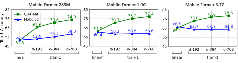
Figure 8: Decoder probing on ImageNet-1K. QB-Heat is on par with MoCo-v2 on linear probing, but outperforms on tran-1 probing. The gain increases as the decoder gets wider.

Here we report decoding probing results on both image classification and object detection. Each task includes multiple decoders. Note that the pre-trained encoders are frozen even when transferring to COCO object detection.

ImageNet classification: Fig. 8 compares QB-Heat with MoCo-v2 [9] on linear and tran-1 probing (see Sec. 5). When evaluating on tran-1 probing, three widths (192, 384, 768) are used in the added transformer block. QB-Heat is on par with MoCo-v2 on linear probing, but is significantly better on tran-1 probing. For instance, when using 192 channels in tran-1 decoder to evaluate pre-trained Mobile-Former-285M, QB-Heat outperforms MoCo-v2 by 12.7% (65.6% vs. 52.9%). This demonstrates that QB-Heat learns stronger non-linear spatial features.

QB-Heat not only works well for decoder probing, but also provides a good initial for fine-tuning. As shown in Tab. 4, its fine-tuning performance consistently outperforms the supervised counterpart over three models. The gain is larger for bigger models. Interestingly, fine-tuning on ImageNet-1K alone (freezing on COCO) boosts detection performance, providing strong task-agnostic encoders.

	head		backbone					AP	AP50	AP75	APS	APM	APL
model	madds	param	model	madds	param	pre-train	IN-ft
	(G)	(M)		(G)	(M)
MF Dec 522	34.6	19.4	MF 3.7G	77.5	25.0	sup	–	40.5	58.5	43.3	21.1	43.4	56.8
						moco2	✗	25.5(-15.0)	40.4	26.7	12.3	27.2	37.0
						moco2	✓	31.7(-8.8)	48.3	33.5	16.1	33.4	45.5
						QB-Heat	✗	43.5 (+3.0)	61.3	47.2	23.2	47.1	60.6
						QB-Heat	✓	45.5 (+5.0)	64.0	49.3	25.2	49.1	63.5
	32.3	18.6	MF 1.0G	20.4	11.7	sup	–	38.3	56.0	40.8	19.0	40.9	54.3
						moco2	✗	30.3(-8.0)	46.0	32.3	15.1	32.1	42.5
						moco2	✓	39.0(+0.7)	56.8	41.8	19.2	41.8	55.3
						QB-Heat	✗	42.6(+4.3)	60.4	46.2	22.7	46.3	59.9
						QB-Heat	✓	44.0(+5.7)	62.5	47.2	23.5	47.6	61.1
	31.1	18.2	MF 285M	5.6	4.9	sup	–	35.2	52.1	37.6	16.9	37.2	51.7
						moco2	✗	31.8(-3.4)	47.8	34.1	14.9	33.3	45.6
						moco2	✓	39.9(+4.7)	57.9	42.7	19.0	43.1	57.1
						QB-Heat	✗	39.7(+4.5)	57.6	42.7	20.4	42.6	56.4
						QB-Heat	✓	41.6(+6.4)	59.2	45.0	21.4	45.2	58.4
MF Dec 211	15.7	9.2	MF 3.7G	77.5	25.0	sup	–	34.1	51.3	36.1	15.5	36.8	50.0
						moco2	✗	12.2(-21.9)	24.1	10.7	5.3	13.0	19.3
						moco2	✓	19.1(-15.0)	33.1	18.4	8.6	19.6	29.3
						QB-Heat	✗	36.7(+2.6)	53.8	39.5	17.2	39.6	53.5
						QB-Heat	✓	41.0(+6.9)	59.3	44.2	20.9	44.5	58.2
	13.4	8.4	MF 1.0G	20.4	11.7	sup	–	31.2	47.8	32.8	13.7	32.9	46.9
						moco2	✗	16.9(-14.3)	29.7	16.4	7.7	17.6	25.8
						moco2	✓	30.6(-0.6)	46.7	32.1	14.4	32.0	45.2
						QB-Heat	✗	35.7(+4.5)	52.5	38.5	16.9	38.6	51.5
						QB-Heat	✓	39.3(+8.1)	56.8	42.0	18.9	43.1	56.3
	12.2	8.0	MF 285M	5.6	4.9	sup	–	27.8	43.4	28.9	11.3	29.1	41.6
						moco2	✗	22.1(-5.7)	35.7	22.8	9.6	22.4	34.4
						moco2	✓	32.7(+4.9)	49.0	34.6	14.5	35.1	48.8
						QB-Heat	✗	33.0(+5.2)	49.3	35.1	15.6	35.2	48.5
						QB-Heat	✓	35.8(+8.0)	52.8	38.3	16.5	38.4	51.5

Table 5: COCO object detection results on val2017 for frozen backbone pre-trained on ImageNet-1K. Evaluation is conducted over three backbones and two heads that use Mobile-Former [12] end-to-end in DETR [5] framework. Our QB-Heat significantly outperforms MoCo-v2 and supervised baselines. Fine-tuning on ImageNet-1K provides consistent improvement. Initial “MF” (e.g. MF-Dec-522) refers to Mobile-Former. “IN-ft” indicates fine-tuning on ImageNet-1K. MAdds is based on the image size 800$\times$1333.

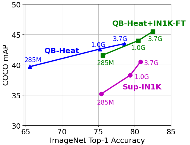
Figure 9: Task-agnostic encoder, evaluated on both ImageNet classification and COCO object detection. Sup-IN1K indicates supervised pre-training on ImageNet-1K. QB-Heat indicates QB-Heat pre-training while QB-Heat+IN1K-FT indicates QB-Heat pre-training followed by fine-tuning on ImageNet-1K. For each pre-training, the three dots correspond to three Mobile-Former backbone variants. When evaluating on image classification, a tran-1 decoder is added on top and learnt from class supervision. When evaluating on object detection, the nine layer head MF-Dec-522 is used and the backbone is frozen. Thus, the backbone is shared by classification and detection tasks. QB-Heat is far behind Sup-IN1K on image classification, but overtakes on object detection. QB-Heat+IN1K-FT boosts detection performance by fine-tuning on ImageNet-1K, providing strong task-agnostic encoders.

COCO object detection: Tab. 5 compares QB-Heat with MoCo-V2 and ImageNet supervised pre-training over three backbones and two heads that use Mobile-Former [12] end-to-end in DETR [5] framework. The backbone is frozen for all pre-training methods. QB-Heat significantly outperforms both MoCo-v2 and supervised counterparts. 2.6+ AP gain is achieved for all six combinations of two heads and three backbones. For the lightest model using Mobile-Former-285M as backbone and MF-Dec-211 as head, 5.2 AP is gained. Similar trend is observed when evaluating in RetinaNet [36] framework (see Tab. 14 in Appendix C). This demonstrates that our QB-Heat learns better spatial representation via quarter-block prediction.

QB-Heat and ImageNet-1K fine-tuning provides strong task-agnostic encoders: Interestingly, fine-tuning on ImageNet-1K alone (but freezing on COCO) after QB-Heat pre-training introduces consistent gain on object detection. As shown in Tab. 5, it gains 1.4–4.3 AP over six combinations of three encoders and two detection decoders. Fig. 9 plots performances of classification and detection that are achieved by sharing encoder weights (or task-agnostic encoder). Although QB-Heat is far behind ImageNet-1K supervised pre-training on classification, it overtakes by a clear margin in detection, showcasing better spatial representation. Fine-tuning on ImageNet-1K boosts performances of both tasks, providing strong task-agnostic encoders. As fine-tuning is performed with layer-wise learning rate decay, it essentially leverages advantages of both QB-Heat (spatial representation at lower levels) and class supervision (semantic representation at higher levels).

Discussion: Compared to QB-Heat, we observe two unexpected behaviors in MoCo-v2, especially when using larger models (MF-1.0G, MF-3.7G). Firstly, the tran-1 probing performance does not improve when using wider decoders (see Fig. 8). Secondly, larger backbones have more degradation in detection performance. As shown in the bottom half of Tab. 5, models with descending size (MF-3.7G, MF-1.0G, MF-285M) have ascending AP (12.2, 16.9, 22.1). We believe this is because MoCo-v2 focuses more on semantics than spatial representation, providing less room for the following tran-1 decoder to improve via spatial fusion. Also, the lack of spatial representation makes it difficult to regress object from sparse queries in DETR. Detailed analysis is provided in Appendix D.

6.4 Fine-tuning on Individual Tasks

Below, we compare with prior works on fine-tuning results of both classification and detection. End-to-end comparison (combining architecture and pre-training) is performed and grouped by computational complexity (FLOPs).

ImageNet-1K classification: Tab. 6 shows that QB-Heat pre-trained Mobile-Former has comparable performance to ViTs pre-trained by either contrastive or MIM methods. This showcases that proper design (quarter masking and linear prediction) of masked image modeling achieves decent performance for CNN based Mobile-Former.

pre-train	encoder	madds	param	fine-tune
MAE-Lite [45]	ViT-Tiny	1.2G	6M	76.1
QB-Heat	MF-285M	0.4G	6M	75.8
QB-Heat	MF-1.0G	1.4G	15M	80.5
iBOT [51]	ViT-S	4.6G	22M	82.3
MoCo-v3 [11]	ViT-S	4.6G	22M	81.4
MAE [25]	ViT-S	4.6G	22M	79.5
CMAE [30]	ViT-S	4.6G	22M	80.2
ConvMAE [22]	ConvViT-S	6.4G	22M	82.6
QB-Heat	MF-3.7G	5.5G	35M	82.5

Table 6: Comparisons with previous results on ImageNet-1K. All self-supervised methods are evaluated by end-to-end fine-tuning. All results are on an image size of 224.

model	query	AP	AP50	AP75	APS	APM	APL	madds	param
								(G)	(M)
DETR-DC5[5]	100	43.3	63.1	45.9	22.5	47.3	61.1	187	41
Deform-DETR[52]	300	46.2	65.2	50.0	28.8	49.2	61.7	173	40
DAB-DETR[38]	900	46.9	66.0	50.8	30.1	50.4	62.5	195	48
DN-DETR[33]	900	48.6	67.4	52.7	31.0	52.0	63.7	195	48
DINO[49]	900	50.9	69.0	55.3	34.6	54.1	64.6	279	47
QB-MF-DETR	100	49.0	67.8	53.4	30.0	52.8	65.8	112	44

Table 7: Comparisons with DETR based models on COCO. QB-MF-DETR uses Mobile-Former (MF-3.7G) as backbone, which has similar FLOPs and model size with ResNet-50 used in other methods. MAdds is based on image size 800$\times$1333.

COCO object detection: Fine-tuning backbone on COCO further boosts detection performance. Tab. 7 shows that QB-MF-DETR (QB-Heat pre-trained Mobile-Former in DETR framework) achieves 49.0 AP, outperforming most of DETR based detectors except DINO [49]. However, our method uses significantly less FLOPs (112G vs. 279G) with significantly fewer object queries (100 vs. 900). Full comparison of fine-tuning results over pre-training methods is reported in Tab. 16 in Appendix C.

7 Discussion

Connection with information theory: Essentially, QB-Heat is a communication system (see Fig. 10) that communicates a quarter of image (via quarter sampling) through linear channels to reconstruct the whole image. It follows the channel capacity in information theory [13] to maximize the mutual information between input and output, but introduces interesting differences in channel, input and optimization (see Fig. 10). Compared to information channel coding, where the channel is probabilistic with fixed parameters (e.g. probability transmission matrix of symmetric channels) and the optimization is over the input distribution $p(x)$, QB-Heat has deterministic linear channel with learnable parameters ($\bm{A}$, $\bm{B}$ in Eq. 1) to optimize.

The key insight is the duality of noise handling between QB-Heat and information channel coding. The channel coding theorem combats noise in the channel by adding redundancy on input $X$ in a controlled fashion, while QB-Heat handles noisy input (i.e. corrupted image) by learning feature representation and spatial redundancy jointly.

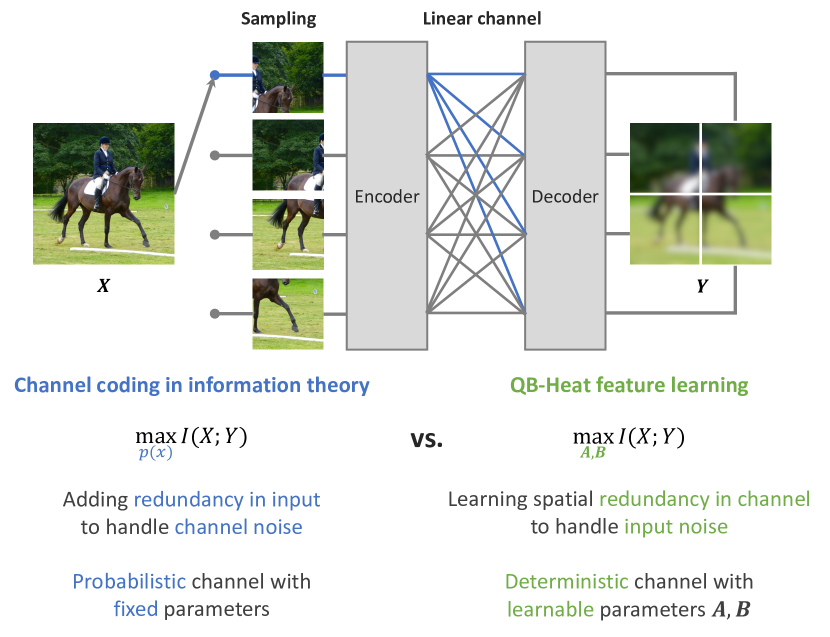
Figure 10: Duality between channel coding in information theory and QB-Heat feature learning. QB-Heat pre-training can be considered as a communication system with quarter sampling and linear channel. Best viewed in color.

Connection with diffusion model: Compared to diffusion models [28, 40, 41] that study noise diffusion along the path from image to noise, QB-Heat studies a different type of diffusion: i.e. the semantic heat diffusion of feature vector across 2D space. But they essentially share a common insight: learning diffusion rate as a function of signal. Specifically, in diffusion model, the noise $\bm{\epsilon}_{t}$ at step $t$ is a function of $\bm{x}_{t}$. In contrast, QB-Heat models the feature change using linear equations as $\frac{\partial\bm{z}}{\partial x}=\bm{A}\bm{z}$, $\frac{\partial\bm{z}}{\partial y}=\bm{B}\bm{z}$.

Limitations: QB-Heat has a major limitation: not working well for vision transformers (ViT). This is mainly due to the discrepancy between pre-training and inference on the range of token interaction. Specifically, QB-Heat does not have a chance to see tokens beyond a quarter-block in pre-training, but all tokens of an entire image are used during inference. This discrepancy becomes more critical for transformers than CNN, as long range interaction is directly modeled via attention in transformer.

8 Conclusion

This paper presents a new self-supervised learning guided by heat equation. It extends heat equation from a single measurable variable to high dimensional latent feature vector, and simplifies it into first order linear differential equations. Based on such simplification, we develop a new masked image modeling (named QB-Heat) that learns to linearly predict three masked quarter-blocks from a single unmasked quarter-block. QB-Heat not only enables masked image modeling for efficient CNN based architectures, but also provides strong task-agnostic encoders on both image classification and object detection. We hope this encourage new understanding of representative feature space by leveraging principles in physics.

Appendix A Derivation of Implicit Linear Models

Below, we show how to derive linear models for implicit directions from explicit directions (see Fig. 5). Let us denote the two explicit models in Eq. 5 along $x$ and $y$ axes (right and down) as $\bm{A}_{1}$ and $\bm{B}_{1}$. Firstly, we derive the models along the negative directions of $x$ and $y$ axes ($\bm{A}_{2}$ and $\bm{B}_{2}$). Then we further extend to 4 diagonal directions ($\bm{C}_{11}$, $\bm{C}_{12}$, $\bm{C}_{21}$, $\bm{C}_{22}$).

Computing $\bm{A}_{2}$ and $\bm{B}_{2}$: Below, we show how to compute $\bm{A}_{2}$ from $\bm{A}_{1}$. $\bm{B}_{2}$ can be derived similarly. The finite difference approximations along opposite directions by using $\bm{A}_{1}$ and $\bm{A}_{2}$ are represented as:

$$\bm{z}(x,y) =(\bm{I}+\Delta x\bm{A}_{1})\bm{z}(x-\Delta x,y)$$

$$\bm{z}(x-\Delta x,y) =(\bm{I}+\Delta x\bm{A}_{2})\bm{z}(x,y).$$ (8)

Thus, $\bm{I}$$+$$\Delta x\bm{A}_{2}$ is the inverse matrix of $\bm{I}$$+$$\Delta x\bm{A}_{1}$. To avoid the difficulty of computing inverse, we approximate $\bm{A}_{2}$ as follows:

$$\bm{A}_{2} =\frac{(\bm{I}+\Delta x\bm{A}_{1})^{-1}-\bm{I}}{\Delta x}\approx-\bm{A}_{1}.$$ (9)

This is used when only two explicit linear models $\bm{A}_{1}$ and $\bm{B}_{1}$ are available (see Fig. 5).

Computing $\bm{C}_{11}$, $\bm{C}_{12}$, $\bm{C}_{21}$, $\bm{C}_{22}$: We show the derivation of $\bm{C}_{11}$ from $\bm{A}_{1}$ and $\bm{B}_{1}$. The other three diagonal directions can be derived similarly. The diagonal prediction of $\bm{z}(x+\Delta x,y+\Delta y)$ from $\bm{z}(x,y)$ can be achieved in two steps (i.e. horizontal prediction followed by vertical) as:

$$\bm{z}(x+\Delta x,y+\Delta y) =(\bm{I}+\sqrt{\Delta x^{2}+\Delta y^{2}}\bm{C}_{11})\bm{z}(x,y)$$

$$=(\bm{I}+\Delta x\bm{A}_{1})\bm{z}(x,y+\Delta y)$$

$$=(\bm{I}+\Delta x\bm{A}_{1})(\bm{I}+\Delta y\bm{B}_{1})\bm{z}(x,y).$$ (10)

The order of horizontal and vertical difference can be flipped as:

$$\bm{z}(x+\Delta x,y+\Delta y) =(\bm{I}+\Delta y\bm{B}_{1})\bm{z}(x+\Delta x,y)$$

$$=(\bm{I}+\Delta y\bm{B}_{1})(\bm{I}+\Delta x\bm{A}_{1})\bm{z}(x,y).$$ (11)

Given that Eq. 10 and Eq. 11 are identical, $\bm{A}_{1}$ and $\bm{B}_{1}$ commute (i.e. $\bm{A}_{1}\bm{B}_{1}=\bm{B}_{1}\bm{A}_{1}$). In practical, $\bm{C}_{11}$ is computed by averaging Eq. 10 and Eq. 11 as follows:

$$\bm{C}_{11} =\frac{\Delta x\bm{A}_{1}+\Delta y\bm{B}_{1}+\Delta x\Delta y(\bm{A}_{1}\bm{B}_{1}+\bm{B}_{1}\bm{A}_{1})/2}{\sqrt{\Delta x^{2}+\Delta y^{2}}}.$$ (12)

Note this computation is needed when using 2 or 4 explicit linear models. (see Fig. 5).

Appendix B Implementation Details

B.1 ImageNet Experiments

Mobile-Former encoders: Tab. 8 shows the network details for three variants of Mobile-Former [12] used in this paper. All of them have 12 blocks and 6 global tokens, but different widths. They are used as encoder (or backbone) for both image classification and object detection. Note that they only have 4 stages and output at resolution ($\frac{1}{16}$), providing more spatial details for translational prediction. These models are manually designed without searching for the optimal architecture parameters (e.g. width or depth).

stage	resolution	block	MF-3.7G		MF-1.0G		MF-285M
			#exp	#out	#exp	#out	#exp	#out
token			6$\times$256		6$\times$256		6$\times$192
stem	2242	conv 3$\times$3	–	64	–	32	–	16
1	1122	bneck-lite	128	64	64	32	32	16
2	562	M-F↓	384	112	192	56	96	28
		M-F	336	112	168	56	84	28
3	282	M-F↓	672	192	336	96	168	48
		M-F	576	192	288	96	144	48
		M-F	576	192	288	96	144	48
4	142	M-F↓	1152	352	288	96	240	80
		M-F	1408	352	704	176	320	88
		M-F	1408	352	704	176	480	88
		M-F	2112	480	1056	240	528	120
		M-F	2880	480	1440	240	720	120
		M-F	2880	480	. 1440	240	720	120
		conv 1$\times$1	–	2880	–	1440	–	720
pool	12	–	–	3136	–	1696	–	912
concat

Table 8: Specification of Mobile-Former encoders. “bneck-lite” denotes the lite bottleneck block [35]. “M-F” denotes the Mobile-Former block and “M-F^↓” denotes the Mobile-Former block for downsampling.

QB-Heat pre-training setup: Tab. 9 shows the pre-training setting. The learning rate is scaled as lr = base_lr$\times$batchsize / 256. We use image size 256 such that the output feature resolution is multiple of 4 (i.e. 16$\times$16). This is required for prediction from the unmasked quarter-block at center position.

Linear probing: Our linear probing follows [25] to adopt an extra BatchNorm layer without affine transformation (affine=False). See detailed setting in Tab. 10.

tran-1 probing: Tab. 11 shows the setting for tran-1 decoder probing. Note that the default decoder widths are 192, 384, 768 for MF-285M, MF-1.0G and MF-3.7G, respectively.

End-to-end fine-tuning: Tab. 12 shows the setting for end-to-end fine-tuning of both encoder and tran-1 decoder. The decoder weights are initialized from tran-1 probing.

config	value
optimizer	AdamW
base learning rate	1.5e-4
weight decay	0.1
batch size	1024
learning rate schedule	cosine decay
warmup epochs	10
image size	2562
augmentation	RandomResizeCrop

Table 9: Pre-training setting.

config	value
optimizer	SGD
base learning rate	0.1
weight decay	0
batch size	4096
learning rate schedule	cosine decay
warmup epochs	10
training epochs	90
augmentation	RandomResizeCrop

Table 10: Linear probing setting.

config	value
optimizer	AdamW
base learning rate	0.0005
weight decay	0.1
batch size	4096
learning rate schedule	cosine decay
warmup epochs	10
training epochs	200
augmentation	RandAug (9, 0.5)
label smoothing	0.1
dropout	0.1 (MF-285M) 0.2 (MF-1.0G/3.7G)
random erase	0 (MF-285M/1.0G) 0.25 (MF-3.7G)

Table 11: tran-1 probing setting.

config	value
optimizer	AdamW
base learning rate	0.0005
weight decay	0.05
layer-wise lr decay	0.90 (MF-285M/1.0G) 0.85 (MF-3.7G)
batch size	512
learning rate schedule	cosine decay
warmup epochs	5
training epochs	200 (MF-285M) 150 (MF-1.0G) 100 (MF-3.7G)
augmentation	RandAug (9, 0.5)
label smoothing	0.1
mixup	0 (MF-285M) 0.2 (MF-1.0G) 0.8 (MF-3.7G)
cutmix	0 (MF-285M) 0.25 (MF-1.0G) 1.0 (MF-3.7G)
dropout	0.2
random erase	0.25

Table 12: End-to-end fine-tuning setting.

B.2 Object Detection in COCO

MF-DETR decoders for object detection: Tab. 13 shows the two decoder structures that use Mobile-Former [12] in DETR [5] framework. Both have 100 object queries with dimension 256. They share similar structure over three scales but have different depths. As the backbone ends at resolution $\frac{1}{16}$, we first perform downsampling (to $\frac{1}{32}$) in the decoder.

stage	MF-Dec-522		MF-Dec-211
query	100$\times$256		100$\times$256
$\frac{1}{32}$	down-conv		down-conv
	M-F+	$\times$5	M-F+	$\times$2
$\frac{1}{16}$	up-conv		up-conv
	M-F-	$\times$2	M-F-	$\times$1
$\frac{1}{8}$	up-conv		up-conv
	M-F-	$\times$2	M-F-	$\times$1

Table 13: Specification of Mobile-Former decoders in COCO object detection. 100 object queries with dimension 256 are used. “down-conv” denotes a downsampling convolutional block that includes a 3$\times$3 depthwise (stride=2) and a pointwise convolution (256 output channels). “up-conv” denotes a upsampling convolutional block that includes bilinear interpolation followed by a 3$\times$3 depthwise and a pointwise convolution. “M-F⁺” and “M-F^-” modify the Mobile sub-block in the original Mobile-Former block. The former replaces it with a transformer block, while the latter uses lite bottleneck [35].

DETR training setup: In decoder probing with frozen bacbkone, only decoders are trained for 500 epochs on 8 GPUs with 2 images per GPU. AdamW optimizer is used with initial learning rate 1e-4. The learning rate drops by a factor of 10 after 400 epochs. The weight decay is 1e-4 and dropout rate is 0.1. Fine-tuning involves additional 200 epochs from decoder probing. Both encoder and decoder are fine-tuned with initial learning rate 1e-5 which drops to 1e-6 after 150 epochs.

Appendix C More Experimental Results

Ablation on training schedule: Fig. 11 shows the influence of the length of training schedule for three Mobile-Former encoders. They share the similar trend: the accuracies of two decoder probings (linear and tran-1) improve steadily as training lasts longer, while fine-tuning with tran-1 achieves decent performance even for pre-training 100 epochs. This is different from MAE [25], in which fine-tuning relies on longer training to improve.

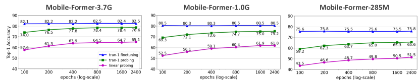
Figure 11: Training schedules. Longer training schedule provides consistent improvement for linear and tran-1 probing over different models, while fine-tuning performance is not sensitive to training schedule.

Decoder probing (frozen backbone) on COCO object detection in RetinaNet framework: Tab. 14 compares QB-Heat with MoCo-V2 and ImageNet supervised pre-training over three backbones in RetinaNet [36] framework. The backbone is frozen for all pre-training methods. Similar to the results in DETR [5] framework (see Sec. 6.3), QB-Heat outperforms both MoCo-v2 and supervised counterparts, demonstrating that our QB-Heat learns better spatial representation via quarter-block prediction. In addition, the followed fine-tuning on ImageNet-1K provides consistent gain.

	head		backbone					AP	AP50	AP75	APS	APM	APL
model	madds	param	model	madds	param	pre-train	IN1K-ft
	(G)	(M)		(G)	(M)
RetinaNet	237.7	61.4	MF-3.7G	77.5	25.0	sup	–	34.0	54.4	35.3	18.7	36.0	46.1
						moco2	✗	29.4(-4.6)	47.8	30.7	20.5	30.7	35.1
						QB-Heat	✗	36.6(+2.6)	55.8	38.6	20.8	39.9	47.7
						QB-Heat	✓	38.7 (+4.7)	59.0	41.0	23.0	42.0	49.9
	178.1	17.2	MF-1.0G	20.4	11.7	sup	–	33.6	54.0	34.9	20.9	35.8	44.4
						moco2	✗	29.3(-4.3)	47.4	30.4	17.6	30.5	37.6
						QB-Heat	✗	35.7(+2.1)	54.7	37.8	20.5	38.8	46.8
						QB-Heat	✓	37.7(+4.1)	57.8	40.0	22.7	40.6	48.8
	163.1	9.5	MF-285M	5.6	4.9	sup	–	30.8	50.0	31.9	17.5	32.4	41.4
						moco2	✗	28.0(-2.8)	45.7	29.2	16.1	29.1	37.7
						QB-Heat	✗	31.3(+0.5)	49.2	33.1	18.1	33.3	42.4
						QB-Heat	✓	33.8(+3.0)	52.6	35.5	19.7	36.4	44.5

Table 14: COCO object detection results on val2017 for frozen backbone pre-trained on ImageNet-1K. Evaluation is conducted over three backbones in RetinaNet [5] framework. Our QB-Heat outperforms MoCo-v2 and supervised baselines. Fine-tuning on ImageNet-1K provides consistent improvement. Initial “MF” (e.g. MF-3.7G) refers to Mobile-Former. “IN1K-ft” indicates fine-tuning on ImageNet-1K. MAdds is based on the image size 800$\times$1333.

Fine-tuning on ImageNet classification with deeper decoders: In Sec. 6.3, we show the results (see Tab. 4) for shallow decoders in image classification (linear lin and single transformer block tran-1). We also find that performance can be further improved by adding more transformer blocks (deeper decoder). Tab. 15 shows the fine-tuning results for using 4 transformer blocks tran-4. Compared with MAE [25] and MoCo [11] on ViT [18], our QB-Heat achieves either similar results with lower FLOPs and fewer parameters, or better performance with similar FLOPs and number of parameters.

pre-train	encoder	decoder	madds	param	fine-tune
MAE-Lite [45]	ViT-Tiny	lin	1.2G	6M	76.1
QB-Heat	MF-285M	tran-4 (d192)	0.7G	7M	78.4
MoCo-v3 [11]	ViT-S	lin	4.6G	22M	81.4
MAE [25]	ViT-S	lin	4.6G	22M	79.5
QB-Heat	MF-1.0G	tran-4 (d384)	2.6G	20M	81.9
MoCo-v3 [11]	ViT-B	lin	16.8G	86M	83.2
MAE [25]	ViT-B	lin	16.8G	86M	83.6
QB-Heat	MF-3.7G	tran-4 (d768)	9.9G	57M	83.5

Table 15: Fine-tuning on ImageNet-1K [14] with deeper decoders. “tran-4 (d192)” denotes the decoder including 4 transformer blocks with 192 channels. All methods are evaluated by end-to-end fine-tuning. All results are on an image size of 224.

Fine-tuning on COCO object detection in DETR framework: Fine-tuning backbone on COCO further boosts detection performance. Tab. 16 shows the full comparison of fine-tuning results that use Mobile-Former [12] end-to-end in DETR [5] framework. Similar to decoder probing with frozen backbone (see Tab. 5 in Sec. 6.3), QB-Heat clearly outperforms MoCo-v2. But different with decoder probing with frozen backbone where QB-Heat outperforms supervised pre-training by a clear margin (see Tab. 5), they are on par in COCO fine-tuning. This is because the advantage of QB-Heat pre-training on spatial representation diminishes as the object labels in COCO provide strong guidance. But QB-Heat can still hold its leading position by leveraging fine-tuning on ImageNet-1K to improve semantic representation and transfer it to object detection. As shown in Tab. 16, compared to supervised pre-training on ImageNet-1K, QB-Heat pre-training followed by ImageNet-1K fine-tuning gains 0.9–2.0 AP over the supervised baseline for all three backbones and two heads.

	head		backbone					AP	AP50	AP75	APS	APM	APL
model	madds	param	model	madds	param	pre-train	IN1K-ft
	(G)	(M)		(G)	(M)
MF-Dec-522	34.6	19.4	MF-3.7G	77.5	25.0	sup	–	48.1	66.6	52.5	29.7	51.8	64.0
						moco2	✗	41.1(-7.0)	59.7	44.6	24.1	44.1	55.5
						QB-Heat	✗	48.0(-0.1)	66.3	52.3	28.1	51.7	64.3
						QB-Heat	✓	49.0 (+0.9)	67.8	53.4	30.0	52.8	65.8
	32.3	18.6	MF-1.0G	20.4	11.7	sup	–	46.2	64.4	50.1	27.1	49.8	62.4
						moco2	✗	41.7(-4.5)	59.8	45.1	24.4	44.7	55.9
						QB-Heat	✗	46.7(+0.5)	64.9	50.8	26.3	50.5	63.4
						QB-Heat	✓	47.1(+0.9)	65.4	51.2	27.5	50.6	63.9
	31.1	18.2	MF-285M	5.6	4.9	sup	–	42.5	60.4	46.0	23.9	46.0	58.5
						moco2	✗	39.6(-2.9)	57.1	42.8	20.9	42.2	55.5
						QB-Heat	✗	42.6(+0.1)	60.8	46.2	22.8	46.2	59.3
						QB-Heat	✓	44.4(+1.9)	62.2	48.1	24.6	47.9	61.7
MF-Dec-211	15.7	9.2	MF-3.7G	77.5	25.0	sup	–	44.0	62.8	47.7	25.8	47.3	60.7
						moco2	✗	35.9(-8.1)	54.0	38.5	19.1	38.8	48.5
						QB-Heat	✗	44.3(+0.3)	62.5	48.1	24.9	47.5	60.8
						QB-Heat	✓	46.0(+2.0)	64.5	49.9	25.5	50.1	62.6
	13.4	8.4	MF-1.0G	20.4	11.7	sup	–	42.5	60.6	46.0	23.6	45.9	57.9
						moco2	✗	33.6(-8.9)	50.4	36.2	17.2	36.2	46.3
						QB-Heat	✗	42.4(-0.1)	60.0	46.0	22.0	45.6	59.8
						QB-Heat	✓	43.8(+1.3)	61.7	47.4	23.7	47.0	60.9
	12.2	8.0	MF-285M	5.6	4.9	sup	–	37.6	55.1	40.4	18.9	40.6	53.8
						moco2	✗	32.3(-5.3)	48.2	34.5	15.4	34.3	46.1
						QB-Heat	✗	37.2 (-0.4)	54.2	39.9	18.4	39.7	53.5
						QB-Heat	✓	39.3(+1.7)	56.8	42.3	19.3	42.0	56.6

Table 16: COCO object detection results on val2017 for fine-tuning backbone. Evaluation is conducted over three backbones and two heads that use Mobile-Former [12] end-to-end in DETR [5] framework. Without using labels in ImageNet-1K, our QB-Heat outperforms MoCo-v2 by a clear margin. When labels in ImageNet-1K is available, QB-Heat pre-training followed by ImageNet-1K fine-tuning outperforms the supervised baselines. Initial “MF” (e.g. MF-Dec-522) refers to Mobile-Former. “IN1K-ft” indicates fine-tuning on ImageNet-1K. MAdds is based on the image size 800$\times$1333.

Appendix D Analysis of Models Pre-trained by MoCo-v2

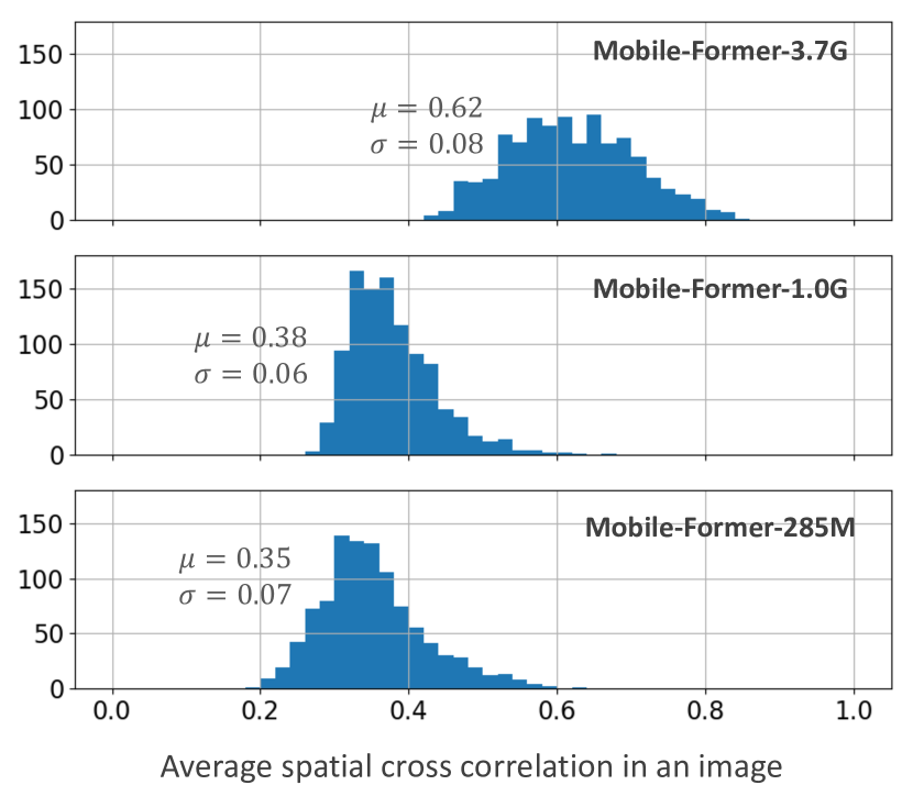
Figure 12: Distribution of spatial correlation in feature maps over 1000 images. The feature maps are extracted by using MoCo-v2 pre-trained models. Larger models have more spatial correlation than smaller models.

Below we provide more analysis related to the two unexpected behaviors (discussed in Sec. 6.3) in the models pre-trained by MoCo-v2. These two behaviors are: (a) the tran-1 probing performance for larger models does not improve when using wider decoders, (b) larger backbones have more degradation in object detection performance.

We observe a clear difference between large and small models in spatial correlation of output feature maps. The spatial correlation for an image is computed as follows. For a given image with size 224$\times$224, the model outputs a feature map with resolution 14$\times$14 over 196 positions. Following Barlow Twins [48], we use cross-correlation matrix $\mathcal{C}$ computed across spatial positions to represent spatial correlation per image. If all positions are highly correlated, each element in $\mathcal{C}$ is close to $\pm$1. In contrast, if positions are not correlated, $\mathcal{C}$ is close to an identify matrix. For each image, we summarize the spatial correlation as the average of absolute values of off-diagonal elements $\frac{1}{N(N-1)}\sum_{i}\sum_{j\neq i}|\mathcal{C}_{ij}|$. Fig. 12 plots the histogram of spatial correlation over 1000 validation images in ImageNet. Clearly, the largest model (MF-3.7G) has significantly more spatial correlation than the smaller counterparts (MF-1.0G, MF-285M).

The larger models have stronger spatial correlation because they are more capable to achieve the goal of contrastive learning, i.e. learning common and discriminative features across multiple views. We conjecture this may limit its capability in spatial representation without explicitly modeling spatial relationship like linear prediction in our QB-Heat. As a result, the following decoders in both image classification and object detection have less room to extract more representative features by fusing different spatial positions. And this disadvantage is enlarged when using DETR in object detection, as it heavily relies on spatial representation to regress objects from sparse queries.

Please note that the difference in spatial correlation (between large and small models) is related to, but not sufficient to explain the degradation of large models in decoder probing (both classification and detection). We will study it in the future work.

Appendix E Visualization

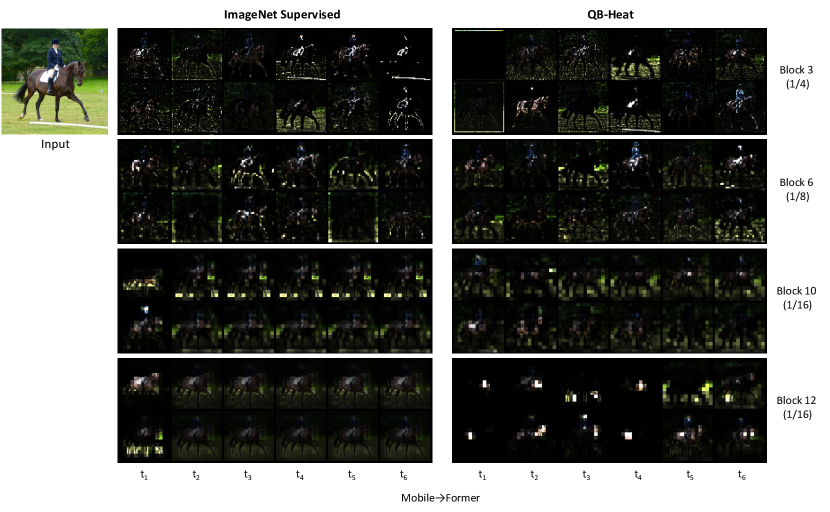
Figure 13: QB-Heat vs. ImageNet supervised pre-training on the cross attention Mobile$\rightarrow$Former. Mobile-Former-3.7G is used, which includes six tokens (each corresponds to a column). Four blocks at different resolutions are visualized and each has two attention heads visualized in two rows. Attention in Mobile$\rightarrow$Former is normalized over pixels, showing the focused region per token. QB-Heat has more diverse cross attentions across tokens (especially at high levels), focusing on different objects (e.g. person, horse, background) and different parts of an object (head, torso, legs of the horse). Best viewed in color.

We also compare our QB-Heat with ImageNet supervised pre-training via visualization of pre-trained models. Following [12], we visualize the cross attention on the two-way bridge (i.e. Mobile$\rightarrow$Former and Mobile$\leftarrow$Former) in Fig. 13 and Fig. 14. Mobile-Former-3.7G is used, which includes six global tokens and eleven Mobile-Former blocks.

Clearly, QB-Heat has more diverse cross attentions across tokens (especially at high levels). Fig. 13 shows the cross attention over pixels in Mobile$\rightarrow$Former. Compared to the supervised pre-training where tokens share the focus on the most discriminative region (horse torso and legs) at high levels (block 10, 12), QB-Heat has more diverse cross attentions, covering different semantic parts. Fig. 14 shows another cross attention in Mobile$\leftarrow$Former over six tokens for each pixel in the feature-map. QB-Heat also has more diverse cross attentions than the supervised counterpart at high levels, segmenting the image into multiple semantic parts (e.g. foreground, background). This showcases QB-Heat’s advantage in learning spatial representation, and explains for its strong performance in multi-task (classification and detection) decoder probing.

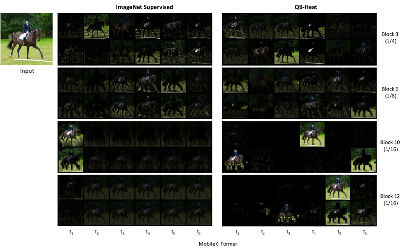
Figure 14: QB-Heat vs. ImageNet supervised pre-training on the cross attention Mobile$\leftarrow$Former. Mobile-Former-3.7G is used, which includes six tokens (each corresponds to a column). Four blocks at different resolutions are visualized and each has two attention heads visualized in two rows. Attention in Mobile$\leftarrow$Former is normalized over tokens showing the contribution of different tokens at each pixel. QB-Heat has more diverse cross attentions across tokens (especially at high levels), segmenting the image into multiple semantic parts (e.g. foreground, background). Best viewed in color.

References

- [1] Mahmoud Assran, Mathilde Caron, Ishan Misra, Piotr Bojanowski, Florian Bordes, Pascal Vincent, Armand Joulin, Michael Rabbat, and Nicolas Ballas. Masked siamese networks for label-efficient learning. arXiv preprint arXiv:2204.07141, 2022.
- [2] Hangbo Bao, Li Dong, and Furu Wei. BEiT: BERT pre-training of image transformers. 2021.
- [3] Adrien Bardes, Jean Ponce, and Yann LeCun. Vicreg: Variance-invariance-covariance regularization for self-supervised learning. In ICLR, 2022.
- [4] S. Becker and G. E. Hinton. A self-organizing neural network that discovers surfaces in random-dot stereograms. Nature, 355:161–163, 1992.
- [5] Nicolas Carion, Francisco Massa, Gabriel Synnaeve, Nicolas Usunier, Alexander Kirillov, and Sergey Zagoruyko. End-to-end object detection with transformers. In ECCV, 2020.
- [6] Mathilde Caron, Hugo Touvron, Ishan Misra, Hervé Jégou, Julien Mairal, Piotr Bojanowski, and Armand Joulin. Emerging properties in self-supervised vision transformers. In Proceedings of the International Conference on Computer Vision (ICCV), 2021.
- [7] Ting Chen, Simon Kornblith, Mohammad Norouzi, and Geoffrey Hinton. A simple framework for contrastive learning of visual representations. arXiv preprint arXiv:2002.05709, 2020.
- [8] Ting Chen, Simon Kornblith, Kevin Swersky, Mohammad Norouzi, and Geoffrey Hinton. Big self-supervised models are strong semi-supervised learners. arXiv preprint arXiv:2006.10029, 2020.
- [9] Xinlei Chen, Haoqi Fan, Ross Girshick, and Kaiming He. Improved baselines with momentum contrastive learning. arXiv preprint arXiv:2003.04297, 2020.
- [10] Xinlei Chen and Kaiming He. Exploring simple siamese representation learning. arXiv preprint arXiv:2011.10566, 2020.
- [11] Xinlei Chen*, Saining Xie*, and Kaiming He. An empirical study of training self-supervised vision transformers. arXiv preprint arXiv:2104.02057, 2021.
- [12] Yinpeng Chen, Xiyang Dai, Dongdong Chen, Mengchen Liu, Xiaoyi Dong, Lu Yuan, and Zicheng Liu. Mobile-former: Bridging mobilenet and transformer. In Proceedings of the IEEE/CVF Conference on Computer Vision and Pattern Recognition (CVPR), 2022.
- [13] Thomas M. Cover and Joy A. Thomas. Elements of Information Theory 2nd Edition (Wiley Series in Telecommunications and Signal Processing). Wiley-Interscience, July 2006.
- [14] Jia Deng, Wei Dong, Richard Socher, Li-Jia Li, Kai Li, and Li Fei-Fei. Imagenet: A large-scale hierarchical image database. In 2009 IEEE conference on computer vision and pattern recognition, pages 248–255. Ieee, 2009.
- [15] Jacob Devlin, Ming-Wei Chang, Kenton Lee, and Kristina Toutanova. BERT: Pre-training of deep bidirectional transformers for language understanding. In Proceedings of the 2019 Conference of the North American Chapter of the Association for Computational Linguistics: Human Language Technologies, pages 4171–4186, Minneapolis, Minnesota, June 2019.
- [16] Xiaoyi Dong, Jianmin Bao, Ting Zhang, Dongdong Chen, Weiming Zhang, Lu Yuan, Dong Chen, Fang Wen, and Nenghai Yu. Peco: Perceptual codebook for BERT pre-training of vision transformers. abs/2111.12710, 2021.
- [17] Xiaoyi Dong, Jianmin Bao, Ting Zhang, Dongdong Chen, Weiming Zhang, Lu Yuan, Dong Chen, Fang Wen, and Nenghai Yu. Bootstrapped masked autoencoders for vision bert pretraining. arXiv preprint arXiv:2207.07116, 2022.
- [18] Alexey Dosovitskiy, Lucas Beyer, Alexander Kolesnikov, Dirk Weissenborn, Xiaohua Zhai, Thomas Unterthiner, Mostafa Dehghani, Matthias Minderer, Georg Heigold, Sylvain Gelly, Jakob Uszkoreit, and Neil Houlsby. An image is worth 16x16 words: Transformers for image recognition at scale. In International Conference on Learning Representations, 2021.
- [19] Aleksandr Ermolov, Aliaksandr Siarohin, Enver Sangineto, and Nicu Sebe. Whitening for self-supervised representation learning. In International Conference on Machine Learning, pages 3015–3024. PMLR, 2021.
- [20] Yuxin Fang, Li Dong, Hangbo Bao, Xinggang Wang, and Furu Wei. Corrupted image modeling for self-supervised visual pre-training. ArXiv, abs/2202.03382, 2022.
- [21] Zhiyuan Fang, Jianfeng Wang, Lijuan Wang, Lei Zhang, Yezhou Yang, and Zicheng Liu. Seed: Self-supervised distillation for visual representation. International Conference on Learning Representations, 2021.
- [22] Peng Gao, Teli Ma, Hongsheng Li, Jifeng Dai, and Yu Qiao. Convmae: Masked convolution meets masked autoencoders. arXiv preprint arXiv:2205.03892, 2022.
- [23] Jean-Bastien Grill, Florian Strub, Florent Altché, Corentin Tallec, Pierre H. Richemond, Elena Buchatskaya, Carl Doersch, Bernardo Avila Pires, Zhaohan Daniel Guo, Mohammad Gheshlaghi Azar, Bilal Piot, Koray Kavukcuoglu, Rémi Munos, and Michal Valko. Bootstrap your own latent: A new approach to self-supervised learning, 2020.
- [24] R. Hadsell, S. Chopra, and Y. LeCun. Dimensionality reduction by learning an invariant mapping. In 2006 IEEE Computer Society Conference on Computer Vision and Pattern Recognition (CVPR’06), volume 2, pages 1735–1742, 2006.
- [25] Kaiming He, Xinlei Chen, Saining Xie, Yanghao Li, Piotr Dollár, and Ross Girshick. Masked autoencoders are scalable vision learners. arXiv:2111.06377, 2021.
- [26] Kaiming He, Haoqi Fan, Yuxin Wu, Saining Xie, and Ross Girshick. Momentum contrast for unsupervised visual representation learning. arXiv preprint arXiv:1911.05722, 2019.
- [27] Kaiming He, Xiangyu Zhang, Shaoqing Ren, and Jian Sun. Deep residual learning for image recognition. In Proceedings of the IEEE conference on computer vision and pattern recognition, pages 770–778, 2016.
- [28] Jonathan Ho, Ajay Jain, and Pieter Abbeel. Denoising diffusion probabilistic models. In H. Larochelle, M. Ranzato, R. Hadsell, M.F. Balcan, and H. Lin, editors, Advances in Neural Information Processing Systems, volume 33, pages 6840–6851. Curran Associates, Inc., 2020.
- [29] Andrew Howard, Mark Sandler, Grace Chu, Liang-Chieh Chen, Bo Chen, Mingxing Tan, Weijun Wang, Yukun Zhu, Ruoming Pang, Vijay Vasudevan, Quoc V. Le, and Hartwig Adam. Searching for mobilenetv3. In Proceedings of the IEEE/CVF International Conference on Computer Vision (ICCV), October 2019.
- [30] Zhicheng Huang, Xiaojie Jin, Chengze Lu, Qibin Hou, Ming-Ming Cheng, Dongmei Fu, Xiaohui Shen, and Jiashi Feng. Contrastive masked autoencoders are stronger vision learners. arXiv preprint arXiv:2207.13532, 2022.
- [31] Li Jing, Jiachen Zhu, and Yann LeCun. Masked siamese convnets. CoRR, abs/2206.07700, 2022.
- [32] Yann LeCun. A path towards autonomous machine intelligence. https://openreview.net/forum?id=BZ5a1r-kVsf, 2022.
- [33] Feng Li, Hao Zhang, Shilong Liu, Jian Guo, Lionel M Ni, and Lei Zhang. Dn-detr: Accelerate detr training by introducing query denoising. In Proceedings of the IEEE/CVF Conference on Computer Vision and Pattern Recognition, pages 13619–13627, 2022.
- [34] Suichan Li, Dongdong Chen, Yinpeng Chen, Lu Yuan, Lei Zhang, Qi Chu, Bin Liu, and Nenghai Yu. Improve unsupervised pretraining for few-label transfer. In Proceedings of the IEEE/CVF International Conference on Computer Vision (ICCV), pages 10201–10210, October 2021.
- [35] Yunsheng Li, Yinpeng Chen, Xiyang Dai, Dongdong Chen, Mengchen Liu, Lu Yuan, Zicheng Liu, Lei Zhang, and Nuno Vasconcelos. Micronet: Improving image recognition with extremely low flops. In International Conference on Computer Vision, 2021.
- [36] Tsung-Yi Lin, Priya Goyal, Ross Girshick, Kaiming He, and Piotr Dollar. Focal loss for dense object detection. In Proceedings of the IEEE International Conference on Computer Vision (ICCV), Oct 2017.
- [37] Tsung-Yi Lin, Michael Maire, Serge Belongie, James Hays, Pietro Perona, Deva Ramanan, Piotr Dollár, and C Lawrence Zitnick. Microsoft coco: Common objects in context. In European conference on computer vision, pages 740–755. Springer, 2014.
- [38] Shilong Liu, Feng Li, Hao Zhang, Xiao Yang, Xianbiao Qi, Hang Su, Jun Zhu, and Lei Zhang. DAB-DETR: Dynamic anchor boxes are better queries for DETR. In International Conference on Learning Representations, 2022.
- [39] Mark Sandler, Andrew Howard, Menglong Zhu, Andrey Zhmoginov, and Liang-Chieh Chen. Mobilenetv2: Inverted residuals and linear bottlenecks. In Proceedings of the IEEE Conference on Computer Vision and Pattern Recognition, pages 4510–4520, 2018.
- [40] Yang Song and Stefano Ermon. Generative modeling by estimating gradients of the data distribution. In Advances in Neural Information Processing Systems, pages 11895–11907, 2019.
- [41] Yang Song, Jascha Sohl-Dickstein, Diederik P Kingma, Abhishek Kumar, Stefano Ermon, and Ben Poole. Score-based generative modeling through stochastic differential equations. In International Conference on Learning Representations, 2021.
- [42] Mingxing Tan and Quoc Le. Efficientnet: Rethinking model scaling for convolutional neural networks. In ICML, pages 6105–6114, Long Beach, California, USA, 09–15 Jun 2019.
- [43] Chenxin Tao, Xizhou Zhu, Gao Huang, Yu Qiao, Xiaogang Wang, and Jifeng Dai. Siamese image modeling for self-supervised vision representation learning, 2022.
- [44] Aäron van den Oord, Yazhe Li, and Oriol Vinyals. Representation learning with contrastive predictive coding. ArXiv, abs/1807.03748, 2018.
- [45] Shaoru Wang, Jin Gao, Zeming Li, Jian Sun, and Weiming Hu. A closer look at self-supervised lightweight vision transformers. arXiv preprint arXiv:2205.14443, 2022.
- [46] Chen Wei, Haoqi Fan, Saining Xie, Chao-Yuan Wu, Alan Yuille, and Christoph Feichtenhofer. Masked feature prediction for self-supervised visual pre-training. In Proceedings of the IEEE/CVF Conference on Computer Vision and Pattern Recognition (CVPR), pages 14668–14678, June 2022.
- [47] Zhirong Wu, Yuanjun Xiong, X Yu Stella, and Dahua Lin. Unsupervised feature learning via non-parametric instance discrimination. In Proceedings of the IEEE Conference on Computer Vision and Pattern Recognition, 2018.
- [48] Jure Zbontar, Li Jing, Ishan Misra, Yann LeCun, and Stéphane Deny. Barlow twins: Self-supervised learning via redundancy reduction. arXiv preprint arXiv:2103.03230, 2021.
- [49] Hao Zhang, Feng Li, Shilong Liu, Lei Zhang, Hang Su, Jun Zhu, Lionel M. Ni, and Heung-Yeung Shum. Dino: Detr with improved denoising anchor boxes for end-to-end object detection, 2022.
- [50] B. Zhou, A. Khosla, Lapedriza. A., A. Oliva, and A. Torralba. Learning Deep Features for Discriminative Localization. CVPR, 2016.
- [51] Jinghao Zhou, Chen Wei, Huiyu Wang, Wei Shen, Cihang Xie, Alan Yuille, and Tao Kong. ibot: Image bert pre-training with online tokenizer. International Conference on Learning Representations (ICLR), 2022.
- [52] Xizhou Zhu, Weijie Su, Lewei Lu, Bin Li, Xiaogang Wang, and Jifeng Dai. Deformable detr: Deformable transformers for end-to-end object detection. arXiv preprint arXiv:2010.04159, 2020.