ClimateNeRF: Extreme Weather Synthesis in Neural Radiance Field

Abstract

Physical simulations produce excellent predictions of weather effects. Neural radiance fields produce SOTA scene models. We describe a novel NeRF-editing procedure that can fuse physical simulations with NeRF models of scenes, producing realistic movies of physical phenomena in those scenes. Our application – Climate NeRF – allows people to visualize what climate change outcomes will do to them.

ClimateNeRF allows us to render realistic weather effects, including smog, snow, and flood. Results can be controlled with physically meaningful variables like water level. Qualitative and quantitative studies show that our simulated results are significantly more realistic than those from SOTA 2D image editing and SOTA 3D NeRF stylization.

1 Introduction

This paper describes a novel procedure that fuses graphic simulations with NeRF models [54, 56] of scenes to produce realistic movies of physical phenomena in those scenes. We apply our method to produce compelling simulations of possible extreme weather outcomes – what would the playground look like after a minor flood? a major flood? a blizzard?

Multi-view Input Images	3D Scene Modeling Sect. 3.1	Neural Scene Stylization Sect. 3.2	Physically-Inspired Simulation Sect. 3.3,  3.4

Figure 2: Method overview. Our method takes multiple posed images, the targeted climate event simulation (e.g., snow), and optionally a user-selected style image as inputs. First, we reconstruct the 3D scene using instant NGP [56] (a variant of NeRF) (Sect. 3.1). The reconstructed radiance fields allow us to synthesize high-quality novel view imagery of the scene efficiently. Second, we optionally finetune the learned instant-NGP model so that it captures the styles of the provided style image (Sect. 3.2). Such 3D consistent stylization is particularly useful for modeling weather effects that are hard to capture via physical simulation. Third, we simulate the climate events by integrating the relevant physical entities (snow, water, smog) to the scene and rendering physically plausible images.

Our application is aimed at an important problem. Cumulative small changes are hard to reason about, and most people find it difficult to visualize what climate change outcomes will do to them  [9, 26, 30, 41]. Steps to slow $\mbox{CO}_{2}$ emissions (say, reducing fossil fuel use) or to moderate outcomes (say, building flood control measures) come with immediate costs and distant benefits. It is hard to support such steps if one can’t visualize their effects.

Traditional graphic simulations can produce realistic weather effects for 3D scenes in a conventional simulation pipeline [71, 22, 31, 100, 16, 20, 28]. But these methods operate on conventional polygon models. Building polygon models that produce compelling renderings from a few images of a scene remains challenging. Neural radiance fields (NeRFs) produce photorealistic 3D scene models from few images [54, 4, 56, 10, 75, 85, 45] but (as far as we know) have rarely been investigated together with graphics simulations. Our method draws from a large literature, reviewed below, that explores editing these models.

Although there are numerous variants of NeRF, most are primarily focused on the task of novel-view synthesis. Directly integrating existing NeRF models for graphics simulation yields unsatisfactory results (Fig. 20). Specifically, we found the geometry of current NeRF models is not sufficiently accurate to enable physics-inspired interactions, and they cannot provide a realistic and complete illumination field to relight the inserted physics entities, such as water and snow. To address this challenge, we have systematically investigated various techniques to improve NeRF models, focusing on answering the critical research question of “what constitutes a good simulatable NeRF representation?”. Our resulting NeRF variant, ClimateNeRF, boasts high-quality geometry, a complete illumination field, and rich semantics, making it particularly well-suited for complex downstream editing and simulation tasks (Sec. 3.1).

ClimateNeRF allows us to render realistic weather effects, including smog, snow, and flood. These effects are consistent over frames so that compelling movies result. At a high level, we: adjust scene images to reflect the global effects of physics; build a NeRF model of a scene from those adjusted images; recover an approximate geometric representation; apply the physical simulation in that geometry; then render using a novel ray tracer. Adjusting the images is essential. For example, trees tend to have less saturated images in winter. We use a novel style transfer approach in an NGP framework to obtain these global effects without changing scene geometry (Sec. 3.2). Our ray tracer merges the physical and NeRF models by carefully accounting for ray effects during rendering (Sec. 3.3). An eye ray could, for example, first encounter a high NeRF density (and so return the usual result); or it could strike an inserted water surface (and so be reflected to query the model again).

We demonstrate the effectiveness of ClimateNeRF in various 3D scenes from the Tanks and Temple, MipNeRF360, and KITTI-360 datasets [4, 37, 44]. We compared to the state-of-the-art 2D image editing methods, such as stable diffusion inpainting [62], ClimateGAN [67]; state-of-the-art 3D NeRF stylization [93]. Both qualitative and quantitative studies show that our simulated results are significantly more realistic than the other competing methods. Furthermore, we also demonstrate the controllability of our physically-inspired approaches, such as changing the water level, wind strength and direction, and thickness of snow and smog.

Our approach results in view consistency (so we can make movies, which is difficult to do with frame-by-frame synthesis); compelling photorealism (because the scene is a NeRF representation); and is controllable (because we can adjust physically meaningful parameters in the simulation). As Fig. 1 illustrates, results are photo-realistic, physically plausible, and temporally consistent.

Our contributions are three-fold:

1. We investigate the challenging problem of repurposing NeRF for realistic simulation and develop a novel framework that can effectively reduce NeRF modeling errors and facilitate graphical simulation.

2. We propose ClimateNeRF, a novel solution that can render realistic weather effects, including smog, snow, and flood, over real-world images.

3. We demonstrate our proposed approach can produce compelling free-viewpoint movies that are photorealistic, geometrically consistent, and controllable.

2 Related Work

Climate simulation: The importance of making climate simulations accessible is well known. [66] collects climate images dataset and performs image editing with CycleGAN [98].  [18, 67] leverage depth information to estimate water mask, and perform GAN-based image editing and inpainting.  [29] simulate fog and snow. These methods offer realistic effects for a single image, but cannot provide immersive, view-consistent climate simulation. In contrast, ClimateGAN allows the view to move without artifacts.

Novel view synthesis: Neural Radiance Field (NeRF) [54, 3, 4, 80] leverage differentiable rendering for scene reconstruction producing photorealistic novel view synthesis. Training and rendering can be accelerated using multiple smaller MLPs and customized CUDA kernel functions [61, 45]. Sample efficiency can be improved by modeling the light field [2] or calculating ray intersections with explicit geometry, such as voxel grids [48, 85, 61], octrees [90], planes [84, 45], and point cloud [87, 101]. Explicit geometric representations improve efficiencies [72, 25, 51, 87, 95]. We build on Instant-NGP [56] as it offers fast learning and rendering, is more memory efficient than grid-like structures, and accelerates our simulation pipeline.

Manipulating neural radiance fields: NeRF entangles lighting, geometry, and materials, making appearance editing hard. A line of work [69, 63, 96, 94, 43, 7, 8] decomposes neural scene representations into familiar scene variables (like environment lighting, surface normal, diffuse color, or BRDF). Each can then be edited with predictable results on rendering. Image segmentation and inpainting can be “lifted” to 3D, allowing object removal [39, 6]. An alternative is to edit source images with text [82]. In contrast, our method does not directly edit the NeRF while producing substantial changes to scene appearance. Geometry editing by transforming a NeRF into a mesh and manipulating that (so editing shapes and compositing) has been demonstrated [88, 92, 15]. In contrast, our method renders the original NeRF together with simulation results.

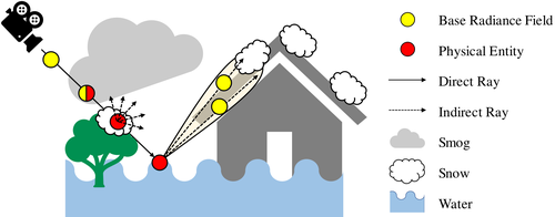
Figure 3: Rendering Procedure of ClimateNeRF. We first determine the position of physical entities (smog particle, snow balls, water surface) with physical simulation. We can then render the scene with desired effects by modeling the light transport between the physical entities and the scene. More specifically, we follow the volume rendering process and fuse the estimated color and density from 1) the original radiance field (by querying the trained instant-NGP model) and 2) the physical entities (by physically based rendering). Our rendering procedure thus maintain the realism while achieving complex, yet physically plausible visual effects.

NGP [56]
Ours
	(a) Normal/Depth/RGB	(b) Smog	(c) Flood	(d) Snow

Figure 4: Climate simulations reveal NeRF modeling errors. Top: NGP, bottom: our NeRF model. On the left, there are normal, depth map, and RGB images. Although the rendered RGB images of the two NeRF versions appear similar, NGP exhibits depth errors in the sky regions and more normal noises on surfaces. This results in geometric inaccuracies in fog and flood images, as well as unrealistic snow accumulation.

Style transfer: Data-driven 2D stylization [35, 58, 32] is a powerful tool to change image color and texture, and can even change the content following masks and labels provided by users [47, 46, 99, 1]. Diffusion models [64, 62, 65] can generate extraordinary image quality based on text input. However, these 2D-based methods cannot currently generate 3D-consistent view synthesis; ours can. Another line of work [14, 12, 93] performs stylization on neural radiance fields. Given an style image, one changes the scene color into the same style. This line of work focuses on artistic effects; in contrast, our changes are driven by physical simulations.

Physically-based simulation of weather: Physical simulation of weather in computer graphics has too long a history to allow comprehensive review here. Fournier and Reeves obtain excellent capillary wave simulations with simple Fourier transform reasoning [23] (and we adopt their method), with modifications by [31, 78];[21] simulates smoke; and [57, 22, 71] simulate snow in wind using metaballs and fluid dynamics. Our method demonstrates how to benefit from such simulations while retaining the excellent scene modelling properties of NeRF style models.

3 Method

ClimateNeRF fuses physical simulations with NeRF models of scenes to produce realistic videos of climate change effects. A simple example illustrates how components interact in our approach. Imagine we wish to build a model of a flooded scene in the Fall. We acquire images, apply a Fall style (Section 3.2), and build a NeRF from the results (Section 3.1). We then use geometric information in that NeRF to compute a water surface. This is represented using a density field, a color field together with normal and BRDF representations (Section 3.3). Finally, to render, we query the model with rays. The details are elaborate (Section 3.4), but the general idea is straightforward: we edit the NeRF’s density and color functions to represent effects like flood; and we intercept rays to represent specular effects. So if a ray encounters high density in the NeRF first, we use the NeRF integral for that ray; but if the first collision is with the water surface, we reflect that ray in the water surface, then query the NeRF with the reflected ray. Fig. 2 provides an overview of our approach.

3.1 Repurposing NeRF for Simulation

NeRF builds a parametric scene representation that supports realistic rendering from multiple images of a scene obtained at known poses. The scene is represented by a field $(\sigma,\mathbf{c})=F_{\theta}(\mathbf{x},\mathbf{d})$, which accepts position $\mathbf{x}$ and direction $\mathbf{d}$ and predicts density $\sigma\in{\mathbb{R}}$ and color $\mathbf{c}\in{\mathbb{R}}^{3}$. This function is encoded in a multi-layer perceptron (MLP) with learnable parameters $\theta$. Rendering is done by querying radiance along appropriate choices of ray, computed as a volume integral [34]. This integral is estimated by drawing samples along the ray, evaluating the density and color of those samples, then accumulating values. The rendering process is differentiable so that NeRF can be trained by minimizing the image reconstruction loss over training views through gradient descent: $\min_{\theta}\sum_{\mathbf{r}}\|C(\mathbf{r})-C_{gt}(\mathbf{r})\|_{2}^{2}$.

(a) Original NeRF	(b) Depth map	(c) Water surface	(d) Normal map with wave	(e) Final ClimateNeRF

Figure 5: Flooding simulation. We first estimate the vanishing point direction based on the original image (a) and depth (b). With the vertical vanishing direction (yellow arrows painted (c)), we can insert a planar water surface $\mathbf{n}_{w}(x-\mathbf{o}_{w})$. We use FFT based water surface simulation to produce a spatiotemporal surface normal map in (d). Our ClimateNeRF renders the scene with the simulated flood through ray tracing NeRF (e).

Repurposing NeRF for simulation:

Although there are numerous variants of NeRF, most are primarily focused on the task of novel-view synthesis [54, 3, 4, 56, 10]. However, combining graphical simulation with these NeRF representations directly results in rendering artifacts, as shown in Fig. 20. These artifacts arise because the NeRF model cannot capture the scene’s accurate and clean geometry, resulting in floaters, and cannot complete the 4D light field, resulting in holes. When physical simulation, such as adding flood and snow into the scene, is incorporated, the artifacts are particularly notable since human perception is more sensitive to these unnatural phenomena.

A good NeRF model for simulation must meet three requirements: 1) accuracy and completeness of geometry, which allows the scene to interact with physical objects; 2) semantic awareness, which enables the interaction to reflect the scene’s characteristics; and 3) coherence and completeness of the light field, which enables the use of NeRF for realistic lighting of the inserted physical entities. To this end, we systematically study multiple variants of techniques to improve NeRF. We use instant-NGP [56] as our base representation to reconstruct the scene for its efficiency and flexibility. This NeRF alternative explicitly stores multi-resolution features for scene representation, making it suitable as we can edit local features easily.

A physical simulation needs access to the surface normal of any point to compute interactions with snow and water, and it needs access to the point’s semantics (in the sense of semantic segmentation) to transfer style. We expand the NGP and allow it to output both semantic logic $\mathbf{s}$ and surface normal $\mathbf{n}$. There is no semantic or surface normal ground truth during training. We use an off-the-shelf pretrained monocular semantic segmentation network [86] to produce semantic maps for each image. We use density gradients $\hat{\mathbf{n}}=-\frac{\nabla\sigma}{\|\nabla\sigma\|}$ [7, 69] (cf. Ref-NeRF [80]) to guide the predicted surface normals $\mathbf{n}$ with a weighted MSE loss.

To simulate (say) a blizzard, we must add snow to the scene and turn trees dark, but we should not change the shape of the house. To keep spatial features intact at the stylization stage, we disentangle instant-NGP’s latent feature (as in [10, 72]). For each voxel in the NGP model, we split the latent feature into geometry features $\gamma_{\text{geo}}$ and appearance features $\gamma_{\text{app}}$. The geometry features are trained to render density. The appearance features are used for rendering color, semantics, and normals. We will freeze the geometry feature vector during the stylization stage and change only the appearance feature vector.

Improving NeRF geometry to reduce simulation errors:

The non-ideal geometry in NeRF, as seen in [54, 56], produces severe artifacts in simulation. To address this issue, we incorporate per-frame appearance embedding [52] and distortion loss [4] to eliminate floaters. Additionally, we utilize a surface normal MLP to enhance the smoothness of the scene normals while introducing a novel sky loss function $\mathcal{L}_{\text{sky}}=\sum_{\mathbf{r}\in\text{sky}}e^{-d(\mathbf{r})}$ to eliminate floaters and fill in holes in the sky. Through these improvements in geometry, we have significantly improved the realism of the simulation (more details can be found in the supplementary material).

Our final NeRF renders density $\sigma$, color $\mathbf{c}$, semantic logit $\mathbf{s}$ and normal $\mathbf{n}$, given a query point and ray direction:

$$(\sigma,\mathbf{c},\mathbf{s},\mathbf{n})=F_{\theta}(\mathbf{x},\mathbf{d};\gamma_{\text{geo}},\gamma_{\text{app}}).$$ (1)

Table. 1 compares the techniques used in NeRF variants and summarize what we find useful to improve the simulation.

Method	Appearance Embed. [52]	Distortion Loss [4]	Predicted Normal	Predicted Semantics [97]	Sky Loss
NGP [56]
Mip-NeRF360 [4]	✓	✓
NeRFacto [76]	✓	✓	✓
Ours	✓	✓	✓	✓	✓

Table 1: Improving NeRF for simulation.

(a) Original NeRF	(b) Surface normal	(c) Metaball centers (red)	(d) Snow with diffuse model	(e) Snow with scattering

Figure 6: Snow simulation. We first locate metaballs on object surfaces facing upward based on surface normal values (b). With metaballs, we can estimate the density $\sigma_{snow}(\mathbf{x})$ and color $\mathbf{c}(\mathbf{x})$ with a parzen window density estimator. (d) and (e) show the differences between fully diffuse model and scattering approximations, shadowed parts in (d) are lit in (e).

3.2 Stylization

Deciduous trees drop their leaves in winter, and physical simulation is not efficient for capturing effects like this. We use FastPhotoStyle [42] to transfer style to rendered images from a pre-trained model $F_{\theta}$. We only transfer only to regions ’terrain’, ’vegetation’, or ’sky’ regions to mimic natural weather change phenomena. The resulting images look realistic but are not necessarily view-consistent. Hence, a student instant-NGP model is fine-tuned to ensure the view consistency of the style-transferred scene. This is trained to minimize the color difference between our student NeRF-rendered results and style-transferred images. We keep the geometry intact and alter only appearance to achieve this goal, so only the appearance feature code $\gamma_{\text{app}}$ is optimized during the style transfer stage: $\min_{\gamma_{\text{app}}}\sum_{\mathbf{r}\in\mathcal{R}}\left\|C(\mathbf{r})-C_{\text{stylized}}(\mathbf{r})\right\|_{2}^{2}$, where $C(\mathbf{r})$ is renderd color and $C_{\text{stylized}}$ is the style-transferred in the same view. This gives us a new NGP model $(\sigma,\mathbf{c}^{\prime})=F_{\theta}^{\prime}(\mathbf{x},\mathbf{d},\ell^{(a)}_{i})$ which encodes the style. This optional style transfer step simulates composite effects, such as a flood in Fall, where the original images were captured in Spring.

3.3 Representing and Rendering Climate Effects

We want to generate scenes with new physical entities – snow, water, smog – in place. We must determine where they are (the job of physical simulation) and what the resulting image looks like (the job of rendering). How the simulation represents results is important because results must be accessible to the rendering process. Rendering will always involve computing responses to ray queries, so computing radiance at $\mathbf{u}$ in direction $\mathbf{v}$. We must represent simulation results in terms of densities, and we must be able to compute normals and surface reflectance properties. Generally, we write $O_{\phi}(\mathbf{x};F_{\theta}):{\mathbb{R}}^{3}\rightarrow{\mathbb{R}}$ for a density resulting from a physical simulation; $N_{\phi}(\mathbf{x};F_{\theta}):{\mathbb{R}}^{3}\rightarrow\mathbb{S}^{2}$ for normals; and $B_{\phi}(\mathbf{x},\bm{\omega}_{o},\bm{\omega}_{i};F_{\theta}):{\mathbb{R}}^{9}\rightarrow{\mathbb{R}}$ for BRDF. Each depends on the existing scene $F_{\theta}$. Choice of $B_{\phi}$ can simulate various effects, including the atmospheric effect of smog, refraction and reflections on water surfaces, and scattering of accumulated snow. $\{O_{\phi},N_{\phi},B_{\phi}\}$ differs drastically across different physical simulations (details per effect in Sect. 3.4).

Once the physical entities are defined by functions $O_{\phi},N_{\phi},B_{\phi}$, we can render them into the image by modeling the light transport between the physical entities and the scene. Given the query point position $\mathbf{x}$, the simulation estimates the density and color of physical entities at position $\mathbf{x}$ through physically based rendering: $\sigma_{\phi}=O_{\phi}(\mathbf{x};F_{\theta})$, $\mathbf{c}_{\phi}=\int_{\Omega}L(\mathbf{x},\bm{\omega}_{i})B_{\phi}(\mathbf{x},\mathbf{d},\bm{\omega}_{i};F_{\theta})(\bm{\omega}_{i}\cdot N_{\phi}(\mathbf{x};F_{\theta}))\text{d}\bm{\omega}_{i}$, where entity color $\mathbf{c}_{\phi}$ is approximated with physically-based rendering equation [33] with normal $N_{\phi}$ and BRDF $B_{\phi}$. Importantly, we approximate the incident illumination $L(\mathbf{x},\bm{\omega}_{i})$ with radiance by tracing a ray $\mathbf{r}(t)=\mathbf{x}-t\bm{\omega}_{i}$ opposite to the incident direction in the learned NeRF, i.e. $L(\mathbf{x},\bm{\omega}_{i})=C(\mathbf{r})$. Depending on the physical entities, we use analytical or sampling-based solutions for the integral. Multiple bounces can be simulated through sampling.

We follow the volumetric rendering process defined in two passes. For every point along a camera ray, we query the opacity and color of the physical entities as described in Sec. 3.3. The system also retrieves the original density $\sigma_{\theta}$ and color $\mathbf{c}_{\theta}$ through Eq. 1. ClimateNeRF estimates final density and color of the simulated scene by: ${\sigma}_{\text{final}}=\sigma_{\theta}+\sigma_{\phi},\quad\mathbf{c}_{\text{final}}=\frac{\sigma_{\theta}\mathbf{c}_{\theta}+\sigma_{\phi}\mathbf{c}_{\phi}}{\sigma_{\theta}+\sigma_{\phi}},$ Once ${\sigma}_{\text{final}},\mathbf{c}_{\text{final}}$ are estimated for each ray points $\{\mathbf{x}_{i}\}$, the pixel color is calculated by volume rendering. Fig. 3 depicts the entire physically inspired simulation and rendering process.

Original	ClimateGAN [67]	Ours

Figure 7: Smog simulation comparison. ClimateNeRF simulate smog in view-consistent manner, and separate foreground objects from background better.

Original	ClimateGAN++ [67]	Stable Diffusion [62]	Ours

Figure 8: Flood simulation comparison. Both ClimateGAN++ [67] and Stable Diffusion [62] inpaint flood using water masks from our reconstructions, but suffer from inaccurate reflections or randomly generated contents. ClimateNeRF simulates photorealistic reflections and ripples.

3.4 Climate Effect Details

ClimateNeRF is able to simulate smog, flood, and snow through various choices of $\{O_{\phi},N_{\phi},B_{\phi}\}$.

Smog Simulation

We assume that smog is formed by tiny absorbing particles, uniformly distributed in empty space. In empty space, the NeRF density $\sigma_{\theta}=0$. The Beer-Lambert law (originally [5, 40]; in [24]) means we can model smog density in free space by simply adding a non-negative constant to the density. Inside high-density regions of the NeRF, adding the constant does not significantly change the integral, so we have $O_{\phi}(\mathbf{x};F_{\theta})=\sigma_{\text{smog}}$. where $\sigma_{\phi}$ decides the density of the smog. Smog particles have a constant color $\mathbf{c}_{\text{smog}}$. Both $\mathbf{c}_{\text{smog}}$ and $\sigma_{\text{smog}}$ are controllable parameters. Fig. 12 depicts the effects of various smog densities.

Flood Simulation

The water surface of the flooded scene is approximately a horizontal plane: $\mathbf{n}_{w}(\mathbf{x}-\mathbf{o}_{w})=0$, where the gravity direction normal $\mathbf{n}_{w}$ is estimated with camera poses and vanishing points detection [50], and plane origin $\mathbf{o}_{w}=(0,0,h)$ determines the water height. But there are water ripples, which we implement following [31] with Fast Fourier Transform (FFT) based ripples and waves. The FFT wave takes random spectral coefficients as input and outputs a spatiotemporal surface normal based on wind speed, direction, and spatial and temporal frequencies. As shown in Fig. 8, compared against still water, FFT-based water surface simulation significantly improves the realism of the water surfaces. We simulate opacity and micro-facet ripples that make the water look glossy (details in supplementary). To approximate the integral of the rendering equation, we adopt the sigma-point method [53, 81] and sample 5 rays from $\mathbf{x}$, including reflection direction $\mathbf{d}_{r}$ and nearby four rays.

(a) (a) Clear water

(b) (b) Muddy water

Figure 9: Refraction in flood simulation

Snow Simulation

Snow is more likely to be accumulated on surfaces facing upward, and the deeper part of the snow is denser due to gravity. We simulate density over object surfaces using metaballs [57, 36] centered on surfaces and with density $\sigma_{o}$ at the center. Realism is ensured by considering both the scene geometry and snowfall direction (e.g., areas such as under the table receiving less accumulated snow). The density distribution within a metaball can be formulated by kernel function $\mathbf{K}(r,R,\sigma_{o})$, which leads to a smooth decrease of density as the distance $r$ from the metaball’s center grows. We follow [79] and tuned it for better quality: $\mathbf{K}(r,R,\sigma)=\frac{315}{64\pi 1.5^{7}}(1.5^{2}-(\frac{r}{R})^{2})^{3}\sigma$.

For any point $\mathbf{x}$ in the space, we calculate the snow’s density of $\mathbf{x}$ using a parzen window density estimator over $N$ local nearest neighbors. The final density of the snow surface is decided accordingly to local geometry (details in supplementary). We use a spatially-varying diffuse color $\mathbf{c}_{\phi}(\mathbf{x}_{i}^{(p)})$ (which is close to pure white multiplied by the average illumination of the scene) to approximate BRDF, and apply a subsurface scattering effect [57] to light the snow’s shadowed part (further detail in supplementary). We re-cast shadows on snow by leveraging 2D shadow prediction [13] and bake shadow map using NeRF geometry. Fig. 6 depicts the snow simulation process.

Original	Swapping Autoencoder [58]	3D Stylization	Ours

Figure 10: Snow simulation comparison. Swapping-Autoencoder [58] captures appearance changes but ignores the geometry of both truck and train. 3D Stylization preserves the geometry of original scene well but doesn’t accumulate snow on horizontal surfaces. In contrast, ClimateNeRF has convincing snow accumulation both on ground and on objects. Note small snow accumulations on the bogies and running board on the train and the boards and bonnet of the truck.

4 Experiments

	Images	Videos
Smog
Flood
Snow

Figure 11: User Study. The bar length indicates the % of users voting for higher realism. The video quality of ClimateNeRF significantly outperforms all baselines.

We evaluate ClimateNeRF and show simulated results over various scenes across different climate effects. We compare our results with state-of-the-art 2D synthesis and 3D stylization to show the quality and consistency of rendered frames. Experimental results demonstrate that our method is more realistic and faithful than existing 2D synthesis and NeRF model finetuned on stylized images while we also maintain temporal consistency and physical plausibility. We encourage readers to watch supplementary videos for a better demonstration of our method’s quality.

4.1 Experimental Details

Datasets.

We conduct experiments on various outdoor scenes: Playground, Family, Horse, Truck, and Train from Tanks and Temples dataset [38], Garden from Mip-NeRF360 [4] and Seq 00 from KITTI-360 [44]. The scenes vary significantly in contents, layouts, and viewpoints.

Baselines.

We compare ClimateNeRF  with the state-of-the-art 2D image editing methods, such as stable diffusion inpainting [62], ClimateGAN [67], as well as state-of-the-art 3D NeRF stylization [93]. For all 2D synthesis approaches, we first build a NeRF using NGP, render at the target view, and conduct synthesis. For all the 3D methods, we re-use the improved version of NGP-based NeRF. ClimateGAN [67] uses monocular depth to predict masks and uses GAN to inpaint the climate-related effects, including smog and flood; ClimateGAN++ is an improved version for flood simulation using our method’s water mask, yielding better geometry consistency; Swapping Autoencoder [58] is a photorealistic 2D style transfer method. We use the model pre-trained on Flickr Mountains dataset and Flickr Waterfall dataset [58] for snow. Stable Diffusion [62] is the state-of-the-art guided image inpainting method based on latent diffusion model. We feed accurate water masks produced by ClimateNeRF  and use text prompts of ”flooding” for inpainting. 3D Stylization leverages FastPhotoStyle [42]. To simulate white snow coverings, we stylize regions labeled road, terrain, vegetation, and sky while keeping the geometry. Please refer to supplementary materials for additional implementation details for all competing methods including ours.

4.2 Experimental Results

Qualitative Results

Fig. 7 depicts qualitative results from smog simulation. Our method delivers better realism and physical plausibility (see the different transmission levels across foreground and background). ClimateGAN [67] generates visually reasonable results but fails to provide sharp boundaries. Additionally, video results further show our method is better at view consistency.

We also report flood simulation results in Fig. 8. ClimateGAN++ [67] produces waters with wrong reflection and blurry artifacts. Stable Diffusion [62] provides realistic and diverse colors and reflectance but hallucinates additional contents (e.g., cars, trees) and lacks consistency. ClimateNeRF renders realistic reflections with Fresnel effects and water ripples. Videos show that ClimateNeRF  is view-consistent and provides fluid dynamics. Fig. 9 shows that our method simulates both clear and muddy water.

We report snow simulation results in Fig. 10. As the figure shows, 3D Stylization changes the floor texture but cannot add physical entities to the scene, limiting its realism. Swapping Autoencoder [58] changes the overall appearance but hallucinates unrealistic textures (e.g., car texture). On the other hand, ClimateNeRF simulates photorealistic winter effects, including accumulated snow and change of sky and tree colors, etc. ClimateNeRF even piles snow on tiny structures like pedals, as shown in the figure.

Figure 12: Controllable Simulation. ClimateNeRF is highly controllable by users. smog density (1st row); flood levels (2nd row); snow accumulations (3rd row).

Using our proposed NeRF significantly enhances the quality of climate simulation. As demonstrated in Fig. 20, comparing to Instant-NGP, our improved geometry results in a more uniform smog density that is aligned with depth, and a more natural intersection between the border of the water surface and the scene. In addition, the appearance of white floaters is reduced and the ground is more evenly covered by snow in the snow scene.

User Study

We perform a user study to validate our approach quantitatively. Users are asked to watch pairs of synthesized images or videos of the same scene and pick the one with higher realism. 37 users participated in the study, and in total, we collected 2664 pairs of comparisons. Results are reported in Fig. 11. ClimateNeRF has consistently been favored among all video simulation comparisons thanks to its high realism and view consistency. Single image comparison does not consider view consistency. In this case, ClimateNeRF still outperforms most baselines except diffusion models on flooding, which also produces realistic water reflectances. Users find diffusion models tend to produce more reflective water surfaces and diverse ripples.

Controllability.

One unique advantage of ClimateNeRF is its controllability. Fig. 12 depicts the changes in smog density, water height, and snow thickness. We show additional controllability results, such as ripple size, flood color, water reflectance, and smog color in supp materials.

Figure 13: Simulation on Driving Scenes [44].

Adverse weather simulation for self-driving.

ClimateNeRF  can be applied to any NeRF scene. In Fig. 13, ClimateNeRF  simulates climate effects in driving scenes of KITTI-360 [44], demonstrating the potential of ClimateNeRF to train and test self-driving under adverse weather.

Limitations

The simulation performance is closely tied to the quality of NeRF. Despite our proposed improvement, there might exist challenging cases leading to simulation artifacts. Additionally ClimateNeRF is not real-time currently, and thus acceleration is an area for future work.

5 Conclusion

We propose a novel NeRF editing framework that applies physical simulation to NeRF models of scenes. Leveraging this framework, we build ClimateNeRF, allowing us to render realistic climate change effects, including smog, flood, and snow. Our synthesized videos are realistic, view-consistent, physically plausible, and highly controllable. We demonstrate the potential of ClimateNeRF to help raise climate change awareness in the community and enhance self-driving robustness to adverse weather conditions.

Supplementary Material

In this supplementary material, we describe implementation details of the simulation framework in Section A and provide an ablation study to validate our design choices in Section B. ClimateNeRF is highly controllable and is demonstrated in Sect C. We present extensive qualitative and quantitative results in Section D and Section E, respectively.

Reconstruction 1	Simulation 1	Reconstruction 2	Simulation 2

Figure 14: Rising Sea-level Simulation. We simulate rising sea level at the Sydney Opera House from various view points.

Reconstruction
Simulation
	La Sagrada Familia	Statue of Liberty	Eiffer Tower	Venice

Figure 15: Rising Sea-level Simulation. Visualizing the consequences of rising sea levels in world-famous scenes [49] can raise general public awareness about climate change.

Appendix A Implementation Details

3D Scene Reconstruction

Our implementation is based on  [59]. We use spatial hashing grid [56] to represent the 3D scene. The entire space contains a multi-resolution feature grid $\{\mathrm{enc}(\mathbf{x};\theta^{l})\}_{l=1}^{L}$, where $L$ is the total number of resolution levels; $\theta^{l}$ are learnable parameters at each level. For a 3D point $\mathbf{x}\in R^{3}$, we index grids by a spatial hash function [77] and fetch feature by interpolation and concatenation: $\gamma=\mathrm{cat}\{\mathrm{interp}(\mathbf{x},\mathrm{enc}(\mathbf{x};\theta^{l}))\}_{l=1}^{L}$. To keep spatial features intact at the stylization stage and separate gradient flows between geometry and color, we develop a disentangled version of instant-NGP inspired by  [10, 72]. Each voxel maintains a geometry code $\gamma_{\sigma}$ and appearance code $\gamma_{\text{app}}$. The geometry code $\gamma_{\sigma}$ encodes opacity and the appearance code $\gamma_{\text{app}}$ contains color, semantic and normal information:

$$\gamma_{\sigma}=\mathrm{cat}\{\mathrm{interp}(\mathbf{x},\mathrm{enc}(\mathbf{x};\theta^{l}_{\sigma}))\}_{l=1}^{L_{\sigma}},\quad\gamma_{\text{app}}=\mathrm{cat}\{\mathrm{interp}(\mathbf{x},\mathrm{enc}(\mathbf{x};\theta^{l}_{app}))\}_{l=1}^{L_{app}}\ ,$$ (2)

where $\mathrm{interp}$ stands for linear interpolation, $\mathrm{cat}$ denotes concatenation.

Inspired by  [56], we use shallow MLPs to predict densities $\sigma$, colors $\mathbf{c}$, semantic logits $\mathbf{s}$ and surface normal values $\mathbf{n}$ respectively from geometry features $\gamma_{\sigma}$ and appearance features $\gamma_{\text{app}}$. We also incorporate low-dimensional per-frame appearance embeddings $\{\ell^{(a)}_{i}\}^{N}_{i=1}$ [52] to balance different lighting conditions across images. With hash grids and MLPs, we have the following function to reconstruct the original scene:

$$(\sigma,\mathbf{c},\mathbf{s},\mathbf{n})=F_{\theta}(\mathbf{x},\mathbf{d},\ell^{(a)}_{i},\gamma_{\sigma},\gamma_{\text{app}})$$ (3)

Following volume rendering and alpha blending [54], we render the color $C(\mathbf{r})$ for ray $\mathbf{r}$ and its semantic logit $S(\mathbf{r})$ [97].

$$C(\mathbf{r})=\sum_{i=1}^{N}T_{i}(1-\text{exp}(-\sigma_{i}\delta_{i}))\mathbf{c}_{i};\quad S(\mathbf{r})=\sum_{i=1}^{N}T_{i}(1-\text{exp}(-\sigma_{i}\delta_{i}))\mathbf{s}_{i},\text{where }T_{i}=\text{exp}\left(-\sum_{j=1}^{i-1}\sigma_{j}\delta_{j}\right)$$ (4)

We apply softmax to semantic logits $S(\mathbf{r})$ to obtain semantic probabilities $\{p(\mathbf{r})^{l}\}_{l=1}^{L}$ for all labels. During training, we perform MSE loss $L_{C}$ and cross-entropy loss $L_{S}$ for rendered colors and semantic logits using ground truth color $C_{gt}(\mathbf{r})$ and 2D semantic logits $\{\hat{p}(\mathbf{r})^{l}\}_{l=1}^{L}$ predicted by segformer [86] pretrained on cityscape dataset [17]. Moreover, since we leverage pseudo-semantic labels, we detach densities $\sigma$ when rendering $S(\mathbf{r})$. Similar to Ref-NeRF [80], we use the density gradient normals $\hat{\mathbf{n}}=-\frac{\nabla\sigma}{\|\nabla\sigma\|}$ [7, 69] to guide the predicted surface normals $\mathbf{n}$ using a weighted MSE loss:

$$L_{C} =\sum_{\mathbf{r}\in\mathcal{R}}\left\|C(\mathbf{r})-C_{gt}(\mathbf{r})\right\|_{2}^{2}\ ,$$ (5)

$$L_{S} =-\sum_{\mathbf{r}\in\mathcal{R}}[\sum_{l\in L}\hat{p}(\mathbf{r})^{l}\log p(\mathbf{r})^{l}]\ ,$$ (6)

$$L_{\mathbf{n}} =\sum_{\mathbf{r}\in\mathcal{R}}\sum_{i=N}^{N}w_{i}\|\mathbf{n_{i}}-\hat{\mathbf{n}}_{i}\|_{2}^{2}\ ,$$ (7)

where $w_{i}=T_{i}(1-\text{exp}(-\sigma_{i}\delta_{i}))$ denotes the detached weight in Eq.4. We also leverage distortion loss $L_{dist}$  [4, 73] to mitigate floaters in the reconstruction results:

$$L_{\text{dist}}= \sum_{i=0}^{N-1}\sum_{j=0}^{N-1}w_{i}w_{j}\left|\frac{t_{i}+t_{i+1}}{2}-\frac{t_{j}+t_{j+1}}{2}\right|+\frac{1}{3}\sum_{i=0}^{N-1}w_{i}^{2}\left(t_{i+1}-t_{i}\right)$$ (8)

However, ngp model tends to create big ’blobs’ in the sky with distortion loss. We alleviate this by applying a simple penalty $L_{sky}=\sum_{\mathbf{r}\in\mathcal{R}}\mathrm{e}^{-D(\mathbf{r})}\cdot\mathbbm{1}\{\hat{p}(\mathbf{r})=\hat{p}_{sky}\}$ where $D(\mathbf{r})$ denotes the depth following Eq. 4 [91] and $\mathbbm{1}\{\cdot\}$ is an indicator function using 2D predicted semantic logits $\hat{p}$. Moreover, we incorporate opacity loss $L_{O}=-\sum_{\mathbf{r}\in\mathcal{R}}O(\mathbf{r})\log O(\mathbf{r})$  [59] to encourage ray opacity being either 0 or 1 to avoid semi-transparent regions in reconstruction results. During our training time, our model’s total loss is a weighted sum of the aforementioned losses:

$$L=L_{C}+\lambda_{S}L_{S}+ \lambda_{\mathbf{n}}L_{\mathbf{n}}+\lambda_{dist}L_{dist}+\lambda_{sky}L_{sky}+\lambda_{O}L_{O}$$ (9)

Transient Object Occlusion

To occlude transient objects like pedestrians or vehicles across views in tanks and temples dataset  [38], we follow  [11] and create per-image learnable masks:

$$M_{i}(u,v)=F_{\psi}(u,v,i,\gamma_{M})\ ,$$ (10)

where $(u,v)\in\mathbb{R}^{2}$, $i$ denotes image coordinates and image index in all training images. $F_{\psi}$ denotes a shallow MLP and $\gamma_{M}$ is the output of hash grids.

In such case, we change color reconstruction loss 5 following  [11]:

$$L_{C}=\sum_{\mathbf{r}\in\mathcal{R}}M(\mathbf{r})\|C(\mathbf{r})-C_{gt}(\mathbf{r})\|^{2}_{2}+\lambda_{M}(1-M({\mathbf{r}}))\ ,$$ (11)

where the second term is used to prevent the mask from predicting everything transient.

Geometry improvements

As mentioned in the limitation subsection in the main paper and can be seen in Fig. 30, ClimateNeRF strongly relies upon high-quality geometry. To improve geometry estimations for KITTI-360 dataset [44], we further use the monocular dense depth $D_{\text{mono}}$ and impose a depth loss:

$$L_{\text{depth}}=\sum_{\mathbf{r}\in\mathcal{R}}\|((wD(\mathbf{r})+d)-D_{\text{mono}}(\mathbf{r}))\|^{2}_{2}\ ,$$ (12)

where $w$ and $d$ are used to align the predicted depth from NeRF $D(\mathbf{r})$ and monocular depth cue $D_{\text{mono}}(\mathbf{r})$ with a least-square criterion [91, 19, 60]. As shown in Fig.16, holes on the ground are “filled” thanks to the supervisions from monocular dense depth.

(a) w/o monocular dense depth $D_{\text{mono}}$	(b) w/ monocular dense depth $D_{\text{mono}}$

Figure 16: Ablation on monocular dense depth supervision Normal estimations in (b) shows that leveraging monocular dense depth removes artifacts on the road.

Training Details

Our implementations of the hash grids and distortion loss follow [55, 59]. For the scale and resolution of the hash grid in our model, we get the inspiration from  [72], where appearance features allocate more grids with finer resolutions. Geometry hash grids have 16 levels and $2^{19}$ entries at most per level, while appearance hash grids have 32 levels and $2^{21}$ entries at most per level. For Tanks and Temples dataset [38] and MipNeRF-360 dataset [4], side length of hash grids is $16$. Geometry MLP and appearance MLP have 128 neurons per layer and one hidden layer, while semantic MLP and normal predicting MLP have 32 neurons per layer and one hidden layer. For our default loss weights in Eq. 9, we set $\lambda_{S}=4^{-2}$, $\lambda_{\mathbf{n}}=7^{-4}$, $\lambda_{dist}=3^{-4}$, $\lambda_{sky}=1^{-1}$ and $\lambda_{O}=2^{-4}$.

A.1 Flood Simulation

Given that water is mostly muddy and non-transparent, we approximate the opacity by checking a point above or under the water’s surface:

$$O_{\phi}(\mathbf{x};F^{\prime}_{\theta})=\begin{cases}\infty&\quad\text{if }\mathbf{n}_{w}(\mathbf{x}-\mathbf{o}_{w})=0\\ 0&\quad\text{otherwise}\end{cases}$$ (13)

Water is highly reflective, yet the microfacet ripples sometimes make the water look glossy. To simulate these effects, we leverage a Spherical Gaussian (SG) to approximate the BRDF on the reflective water surface:

$$B_{\phi}(\mathbf{x},-\mathbf{d},\bm{\omega}_{i},N_{\phi}(\mathbf{x}))=\exp^{\lambda(-\bm{\omega}_{i}\cdot\mathbf{d}_{r}-1)}$$ (14)

where SG lobe axis is $\mathbf{d}_{r}=\mathbf{d}-2(\mathbf{d}\cdot N_{\phi}(\mathbf{x}))N_{\phi}(\mathbf{x})$,, and $\lambda\in{\mathbb{R}}_{+}$ is the lobe sharpness, controlling the glossy effects.

We use sigma point-based sampling for rendering water. Specifically, the camera ray $\mathbf{r}(t)=\mathbf{o}+t\mathbf{d}$ is cast from the camera and hits the water surface at position $\mathbf{x}$. We compute the observed color by a sampling-based approximation of the rendering equation:

$$\mathbf{c}_{\phi}=(1-R)\mathbf{c}_{w}+R\displaystyle\sum_{i=1}^{5}L(\mathbf{x},\bm{\omega}_{i})e^{\lambda(-\bm{\omega}_{i}\cdot\mathbf{d}_{r}-1)},$$ (15)

where $L(\mathbf{x},\bm{\omega}_{i})=C(\mathbf{r})$ is the NeRF ray color (Eq. 4), representing the incident light color hitting $\mathbf{x}$ along direction $\bm{\omega}_{i}$. $R\in(0,1)$ is the reflectance index determined by viewing direction $d$ and normal $N_{\phi}(\mathbf{x})$, which enables the system to simulate the Fresnel effect on the water. To approximate the integral in rendering equation [33], we adopt the sigma-point method [53, 81] and sample 5 rays from the position $\mathbf{x}$, including reflection direction $\mathbf{d}_{r}$ and nearby four rays. In short, ClimateNeRF simulates Fresnel effect, glossy reflection, and wave dynamics.]

Fresnel Effect

When the light hits the water’s surface, the amount of reflection and transmission is determined by the incident and normal directions and is described by the Fresnel effect. The angle between normal and incident rays is denoted by $\theta_{i}$, and the angle between normal and refracted ray in water is $\theta_{t}$. According to Snell’s Law: $r_{i}\theta_{i}=r_{t}\theta_{t}$, where $r_{i}=1$ is the refraction index of air and $r_{t}=1.33$ is the refraction index of water in our experiments, which is also consistent with real-world water properties. Next, the reflectance $R$ in Eq. 15 is computed by:

$$R=\frac{R_{s}+R_{p}}{2},\quad R_{s}=\left[\frac{\text{sin}(\theta_{t}-\theta_{i})}{\text{sin}(\theta_{t}+\theta_{i})}\right]^{2},\quad R_{p}=\left[\frac{\text{tan}(\theta_{t}-\theta_{i})}{\text{tan}(\theta_{t}+\theta_{i})}\right]^{2}$$ (16)

where $R_{s}$ and $R_{p}$ are the reflectances for s-polarized and p-polarized light, respectively. Modeling the Fresnel effect in our flood simulation pipeline makes the water far from the camera (larger $\theta_{i}$) have higher $R$ and looks more like a mirror. The water nearby (smaller $\theta_{i}$) has lower $R$ and shows watercolor, enhancing the simulation’s realism.

Refraction Effect

Refraction occurs when light transports from one medium to another. Modeling such an effect helps simulate clear water. With a ray direction, surface normal, and refraction index $r_{t}$ of the water, ClimateNeRF calculates the refraction direction $\bm{\omega}_{t}$ according to Snell’s Law, and retrieves color with volume rendering along $\bm{\omega}_{t}$. Next, we can simulate underwater scenes following  [68].

$$\mathbf{c}_{\phi}=(1-R)(t_{c}(\mathbf{x})L(\mathbf{x},\bm{\omega}_{t})+(1-t_{c}(\mathbf{x})\mathbf{c}_{w})+R\displaystyle\sum_{i=1}^{5}L(\mathbf{x},\bm{\omega}_{i})e^{\lambda(-\bm{\omega}_{i}\cdot\mathbf{d}_{r}-1)},$$ (17)

where $t_{c}(\mathbf{x})=e^{-\beta_{c}D(x,\bm{\omega}_{t})}$ and $D(x,\bm{\omega}_{t})$ denotes the geometry depth alone refraction direction. Consequently, ClimateNeRF can simulate reflection and refraction, simulating clear and muddy water with controllable parameter $\beta_{c}$.

A.2 Snow Simulation

For any point $\mathbf{x}$ in the space, we calculate the snow’s density of $\mathbf{x}$ in a particle-based manner. We first figure out a set of $N$ particles as metaballs’ centers $\{\mathbf{x}^{(p)}_{i}\}_{i=1}^{N}$ with densities $\{\sigma^{(p)}_{i}\}_{i=1}^{N}$ and metaball radius $\{R^{(p)}_{i}\}_{i=1}^{N}$ around $\mathbf{x}$. Then we sum up the densities calculated by kernel function $\mathbf{K}(r,R,\sigma_{o})$.

$$\begin{split}\sigma_{\text{snow}}(\mathbf{x})&=\sum_{i=1}^{N}\sigma_{\mathbf{K}}(\mathbf{x},\mathbf{x}^{(p)}_{i}),\\ \text{where }\sigma_{\mathbf{K}}(\mathbf{x},\mathbf{x}^{(p)}_{i})&=\mathbf{K}(\|\mathbf{x}-\mathbf{x}^{(p)}_{i}\|_{2},R^{(p)}_{i},\sigma^{(p)}_{i})V_{g}(\mathbf{x}^{(p)}_{i},\bm{\omega}_{s}),\end{split}$$ (18)

where $\sigma^{(p)}_{i}$ is defined by weights during volume rendering 4 for $\sigma_{\theta}$ of $F^{\prime}_{\theta}$. More details are shown in Section A.3. We denote $V_{g}(\mathbf{x}^{(p)}_{i},\bm{\omega}_{s})$ as the transparency along snow falling direction $\bm{\omega}_{s}$ retrieved from a pre-trained visibility network based on pre-trained NeRF’s geometry to simulate snow occlusions. When training the visibility network, we perturb snow-falling directions within a small angle to soften snow boundaries. During rendering, we identify snow surface by a threshold $\tau_{\text{snow}}$ and a hyperparameter $a$:

$$O_{\phi}(\mathbf{x};F^{\prime}_{\theta})=\frac{1}{1+e^{-a(x\sigma_{\text{snow}}-\tau_{\text{snow}})}}\sigma_{\text{snow}},$$ (19)

The BRDF of snow particles is set as spatially-varying diffuse color $\mathbf{c}_{\phi}(\mathbf{x}_{i}^{(p)})$ close to pure white multiplied by the average illumination of the scene. Furthermore, since the snow is semi-transmissive, the subsurface scattering effect [57] will light the snow’s shadowed part. To simulate such effect, we leverage warp lighting function [27] $\Phi(\mathbf{n}_{\mathbf{K}},\mathbf{n}_{l},\gamma_{\Phi})$ based on normalized surface normal $\mathbf{n}_{\mathbf{K}}$, light vector $\mathbf{n}_{l}$ and hyperparameter $\gamma_{\Phi}$. We use 2D shadow predictions [13] and bake shadow confidence $V_{s}(\mathbf{x})\in[0,1]$ on pre-trained NeRF’s geometry using $L_{2}$ loss. For an arbitrary point $\mathbf{x}$ in space, the color of point $\mathbf{x}$ is a weighted sum of $\{\mathbf{c}^{(p)}_{i}\in{\mathbb{R}}^{1}\}_{i=1}^{N}$ based on kernel function:

$$\begin{split}\mathbf{c}_{\phi}(\mathbf{x})&=\frac{\sum_{i=1}^{N}\sigma_{\mathbf{K}}(\mathbf{x},\mathbf{x}^{(p)}_{i})\frac{\mathbf{c}^{(p)}_{i}+\mathbf{c}_{0}}{1+\mathbf{c}_{0}}(\beta_{s}V_{s}(\mathbf{x}^{(p)}_{i})+V_{s0})}{\sum_{i=1}^{N}\sigma_{\mathbf{K}}(\mathbf{x},\mathbf{x}^{(p)}_{i})}\Phi(\mathbf{n}_{\mathbf{K}}(\mathbf{x}),\mathbf{n}_{l},\gamma_{\Phi})\ ,\end{split}$$ (20)

where $\Phi(\mathbf{n}_{\mathbf{K}}(\mathbf{x}),\mathbf{n}_{l},\gamma_{\Phi})=\frac{\mathbf{n}(\mathbf{x})\cdot\mathbf{n}_{l}+\gamma_{\Phi}}{1+\gamma_{\Phi}}$ and $\frac{\mathbf{c}^{\prime(p)}_{i}+\mathbf{c}_{0}}{1+\mathbf{c}_{0}}$ is used to approximate a high albedo for snow and $\mathbf{c}_{0}$ is a hyperparameter. To recast shadow on snow, we let $\beta_{s}$ and $V_{s0}$ in Eq. 20 be hyperparameters. See Figure 26 for example. Surface normal values of metaballs are still calculated in a gradient-based manner. Moreover, we stylize the scene to match the color tones of different weather conditions, as shown in Fig. 27.

A.3 Extensions

Bake Editing

When simulating physical entities, especially snow, rendering will be time-consuming if we straightly let snow fall from the sky and do collision detection. Moreover, a lack of supervision in a bird’s eye view makes depth estimation for rays cast from the sky inaccurate. To mitigate the aforementioned issues, we fit the distribution of metaballs’ densities and colors in a new model and fetch them in a particle-based manner. The new model outputs high densities where metaballs locate. We use $w_{i}=T_{i}(1-\text{exp}(-\sigma_{i}\delta_{i}))$ in Eq. 4 for surface detection since $w(\mathbf{x})\in[0,1]$ is close to 1 when $\mathbf{x}$ is close to surfaces. To identify surfaces where snow accumulates, we incorporate surface normals $\mathbf{n}$ and vertical axis $\mathbf{n}_{\perp}$ to figure out metaballs’ density weights: $w^{(p)}_{i}=\frac{1}{1+e^{-a^{\prime}(\mathbf{n}_{i}\cdot\mathbf{n}_{\perp}-\cos(\theta_{0}))}}w_{i}$ where $\theta_{0}$ is a hyperparameter. We then bake $w^{(p)}_{i}$ into a new model $G_{\phi_{w}}$:

$$w^{(p)}_{\phi_{w}}(\mathbf{x})=G_{\phi_{w}}(\mathbf{x})$$ (21)

We also bake the gray scale [70] of $\mathbf{c}_{\theta}$ from $F_{\theta}$ into a new model $G_{\phi_{\mathbf{c}}}$ to capture an approximation for light intensities and shadows:

$$\mathbf{c}^{(p)}_{\phi_{\mathbf{c}}}(\mathbf{x})=G_{\phi_{\mathbf{c}}}(\mathbf{x})$$ (22)

(a) Sample near a large surface	(b) Sample near a tiny surface

Figure 17: Visualization of voxel+nest sampling for $N_{n}=3$. Instead of storing metaball information in point cloud, we approximate metaball’s center density distributions with $G_{\phi_{w}}$. Our voxel+nest sampling helps capture different geometric level of details [74], which makes large metaballs dominate at flat surfaces, and put smaller snow balls on thin structures.

Then, we leverage the pre-trained $G_{\phi_{w}}$, $G_{\phi_{\mathbf{c}}}$ and do voxel sampling to fetch $\{\sigma^{(p)}_{i}\}_{i=1}^{N}$ and $\{\mathbf{c}^{(p)}_{i}\}_{i=1}^{N}$ from 8 vertices. Also, to automatically alter metaballs’ radiuses according to the size of the surface, we sample nested grids with different side lengths defined in a geometric progression. Moreover, we define metaballs’ radiuses by girds’ side lengths. Hence, Eq. 18 and Eq. 20 can be rewritten as:

$$\sigma_{\text{snow}}(\mathbf{x})=\sum_{i=1}^{8N_{n}}\sigma_{\mathbf{K}}(\mathbf{x},\mathbf{x}^{(p)}_{i});\quad\mathbf{c}_{\phi}(\mathbf{x})=\frac{\sum_{i=1}^{8N_{n}}\sigma_{\mathbf{K}}(\mathbf{x},\mathbf{x}^{(p)}_{i})\frac{\mathbf{c}^{(p)}_{i}+\mathbf{c}_{0}}{1+\mathbf{c}_{0}}(\beta_{s}V_{s}(\mathbf{x}^{(p)}_{i})+V_{s0})}{\sum_{i=1}^{8N_{n}}\sigma_{\mathbf{K}}(\mathbf{x},\mathbf{x}^{(p)}_{i})}\Phi(\mathbf{n}_{\mathbf{K}}(\mathbf{x}),\mathbf{n}_{l},\gamma_{\Phi}),$$ (23)

where $N_{n}$ is the number of nests. We calculate density $\sigma^{(p)}$ and albedo color $\mathbf{c}^{(p)}$ for metaball centered at $\mathbf{x}^{(p)}$ by $\sigma^{(p)}=w^{(p)}_{\phi_{w}}(\mathbf{x}^{(p)})\sigma_{0}$ and $\mathbf{c}^{(p)}=\mathbf{c}^{(p)}_{\phi_{\mathbf{c}}}(\mathbf{x})$ where $\sigma_{0}$ is a hyperparameter. See Fig. 17 for a visualization of this sampling strategy. If stylization is done on the scene, we leverage the stylized model $F^{\prime}_{\theta}$ and finetune the $G_{\phi_{\mathbf{c}}}$ to match new illumination conditions while remaining $G_{\phi_{w}}$ intact since $F^{\prime}_{\theta}$ shares the same spatial information with $F_{\theta}$.

Anti-Aliasing

When rendering with simulation, the high-frequency normal map changes on the physical entity surface would lead to an aliasing effect. To alleviate such artifacts, we can render four times larger images with higher resolution and perform anti-aliasing downsampling to the original resolution.

Appendix B Ablation Study

To justify our design choices, we perform an ablation study of flood simulation, and the results are shown in Fig 18. Specifically, we report the simulation results without certain technical components depicted in Sec. A.1 of the main paper.

Fig 18 shows that all components are essential for realism. For example, vanishing point detection [50] makes the water plane follow gravity direction; wave simulation adds ripples to the water surface; the Fresnel effect makes the water reflectance view-dependent and physically plausible; the Glossy effect mimics realistic microfacet water surfaces with ripples; anti-aliasing removes far-away high-frequency noises. In short, all components contribute to the realism of the simulation.

We also perform an ablation study on snow simulation to validate our approximate scattering rendering in Fig. 19. We compare 1) pure white metaballs with spatial variant colors, 2) metaballs in a fully diffuse model, and 3) our full simulation. Results demonstrate that our choice provides a more realistic rendering of accumulated snow.

To identify how scene geometry improvements benefit simulations, the ablation study of various technical components is illustrated in Fig. 20. For example, appearance embeddings mitigate the floaters caused by varying exposures in training views, and sky loss reduces blobs in the sky. Results show that our improvements in geometry reconstructions help simulate dense snow covering in both foreground and background, thus offering more visually pleasing results.

(a) Inaccurate plane geometry	(b) No wave simulation	(c) No Fresnel effect
(d) No glossy effect	(e) No anti-aliasing	(f) Full simulation

Figure 18: Ablation Study of Flood Simulation. (a) Without accurate plane geometry estimation with vanishing point detection [50], the water surface deviates from gravity direction. (b) The surface is perfect planar without wave simulation, which is not natural. (c) Fresnel effect makes the water far from the camera (with a larger incident angle) have higher reflectance, and is consistent with physical rules. (d) The glossy effect makes the reflection more blurry and realistic (e) There is much high-frequency noise around the water border without an anti-aliasing trick. (f) Our full flood simulation results.

Pure White Snow	Only spatial variant colors	Only diffuse model	Full model

Figure 19: Ablation Study for Snow Simulation Though spatial variant colors capture local illumination conditions, they fail to offer a sense of depth for snow. Moreover, the diffuse model cannot simulate snow’s scattering effects.

NGP [56]
w/o appearance embedding
w/o distortion loss
w/o normal predictions
w/o sky loss
Ours
	(a) Normal/Depth/RGB	(d) Snow

Figure 20: Geometry Improvement for Simulation. Appearance embeddings [52] and distortion loss [4] mitigate floaters or incomplete geometries while normal prediction loss [80] smooths predicted normals and leads a well interpolation in background(see the snow coverage in the background). Sky loss offers primitives for sky depth and alleviates ’blobs’ in the sky.

Appendix C Controllability

We further demonstrate that ClimateNeRF is highly controllable during the simulation process. In Fig. 21, our method simulate different colors of smog and flood, water clearness, varying spatial frequency of water ripples, and distinct heights of accumulated snow. The results show that our simulation framework is highly controllable by the users. Consequently, scientists can use this framework to simulate accurate climate conditions depending on the projected climate in the future and visualize the consequences corresponding to different actions taken by policymakers and the general public.

Figure 21: Controllable Climate Simulation. From the top row to the bottom row, we control (1) smog color (2) water clearness (3) watercolor (4) spatial frequency of the wave. The frequency decreases from left to right. (5) snow height. We control snow height by adjusting the threshold density $\tau_{\text{snow}}$.

Appendix D Qualitative Results

We demonstrate more qualitative results is Fig. 22, Fig. 23, Fig. 24, Fig. 25, and Fig. 26. For smog scene images in Fig. 22, ClimateGAN [67] generates visually plausible results but fails to provide sharp boundaries, and 3D stylization attempts to change the surface texture but makes the images overall darker. Our method simulates realistic visibility reduction effects caused by smog, thanks to the geometry reconstruction.

The flood images are shown in Fig. 23. ClimateGAN++ [67] cannot reconstruct realistic reflection on the water surface, Stable Diffusion [62] synthesize realistic water appearance but also produce random objects (e.g., cars, signs) in the scene, which is not consistent across views. ClimateNeRF simulates realistic reflection and water ripples while being view-consistent. This is better demonstrated in the supp video and website. In Fig. 24, we compare with other NeRF-editing baselines. We first edit training images with ClimateGAN [67] or 2D stylization [42] and optimize the neural radiance field. While these baseline methods produce more view-consistent rendering, they either generate severe floating artifacts to compensate for the image inconsistency or cannot perform geometric editing, which sabotages realism.

We also compare our FastPhotoStyle [42] based stylization method with Artistic Radiance fields [93]. As shown in Fig. 28, we sustain more appearance details from the original scene. ClimateNeRF can apply flood simulation pipeline to synthesize rising sea levels in large-scale scenes, as shown in Fig. 14, 15. Visualizing the consequences of such effects can raise general public awareness and call for government actions against climate change

Original	ClimateGAN [67]	3D Stylization	Ours

Figure 22: Smog simulation comparison.

Original	ClimateGAN++ [67]	Stable Diffusion [62]	Ours

Figure 23: Flood simulation comparison.

Original	ClimateGAN [67]+NeRF	3D Stylization	Ours

Figure 24: NeRF editing for flood simulation. We tested the ClimateGAN image + NeRF training baseline, but the results are blurry due to inconsistent inputs. 3D stylization baseline is a NeRF trained on stylized images.

Original	Swapping Autoencoder [58]	3D stylization	Ours

Figure 25: Snow simulation comparison.

Figure 26: Simulation on Urban Driving Scenes.

(a) Original NeRF rendering	(b) Original NeRF + snow	(c) NeRF with stylization	(d) NeRF with stylization + snow

Figure 27: Stylization. Performing snow simulation with the original NeRF model leads to incompatible scene appearance (e.g., snow on green vegetations). We address this issue by first finetuning the appearance of the NeRF model to match the style of the provided style image. Our snow simulation on the stylized NeRF model shows visually more appealing results.

Style Image from  [89]	Original	ARF  [93]	3D stylization

Figure 28: Comparison with Artistic Radiance Fields [93]

ClimateGAN++ [67]
Stable Diffusion [62]
Ours
	$t=0$	$t=40$	$t=80$	$t=120$	$t=160$

Figure 29: View Consistency Comparison. We show flood simulation in Playground scene and time step $t$ increases from left to right. ClimateGAN++ [67] (Top) cannot generate realistic reflection, Stable Diffusion [62] (Middle) synthesizes different objects in each views. Ours (Bottom) simulate photorealistic and consistent reflection and ripples.

(a) Original NeRF rendering	(b) Climate NeRF rendering	(c) Depth rendering	(d) Surface normal rendering

Figure 30: Limitations. Snow simulation on KITT-360 [44] dataset fails to cover a shadowed road due to wrong geometry.

Appendix E Quantitative Results

No automatic quantitative score can holistically evaluate the quality of our weather-simulated movies. In this project, we evaluate the synthesized videos with the state-of-the-art video quality assessment model UVQ [83] and report the results in Table 2. The score ranges between interval $(1,5)$, where 1 indicates the lowest quality and 5 indicates the highest quality. As the table shows, our smog simulation outperforms all other baselines, while it does not win Stable Diffusion [62] in flood simulation and ClimateGAN [67] in snow simulation. That being said, UVQ prefers sharp videos instead of measuring holistic realism. As shown in Fig. 25, baselines get a better quality score despite providing low-quality snow simulation results, suggesting UVQ might not be a good metric for our task. Hence, despite demonstrating UVQ [83] results, we want to emphasize that such metrics mainly focus on measuring the amount of low-level degradation (such as blurriness and noise), which cannot faithfully reproduce human evaluation on realism. Having a good video quality score on simulation remains an open topic.

		Smog			Flood				Snow
	Original	GAN	3D Style	Ours	GAN	GAN++	Diffusion	Ours	GAN	3D Style	Ours
Family	3.434	3.426	3.425	3.437	3.408	3.413	3.416	3.424	3.434	3.434	3.431
Horse	3.426	3.422	3.422	3.432	3.409	3.412	3.416	3.422	3.435	3.424	3.421
Playground	3.409	3.402	3.403	3.412	3.400	3.402	3.409	3.404	3.427	3.412	3.415
Train	3.406	3.396	3.407	3.407	3.401	3.402	3.410	3.407	3.417	3.411	3.408
Truck	3.425	3.424	3.424	3.431	3.404	3.403	3.424	3.413	3.431	3.424	3.416

Table 2: Video Quality Assessment. We evaluate the video quality with Google’s Universal Video Quality (UVQ) model [83].

References

- [1] Rameen Abdal, Yipeng Qin, and Peter Wonka. Image2stylegan++: How to edit the embedded images? In CVPR, 2020.
- [2] Benjamin Attal, Jia-Bin Huang, Michael Zollhöfer, Johannes Kopf, and Changil Kim. Learning neural light fields with ray-space embedding. In CVPR, pages 19819–19829, 2022.
- [3] Jonathan T Barron, Ben Mildenhall, Matthew Tancik, Peter Hedman, Ricardo Martin-Brualla, and Pratul P Srinivasan. Mip-nerf: A multiscale representation for anti-aliasing neural radiance fields. In ICCV, 2021.
- [4] Jonathan T Barron, Ben Mildenhall, Dor Verbin, Pratul P Srinivasan, and Peter Hedman. Mip-nerf 360: Unbounded anti-aliased neural radiance fields. In CVPR, 2022.
- [5] Beer. Bestimmung der absorption des rothen lichts in farbigen flüssigkeiten. Annalen der Physik und Chemie, 1852.
- [6] Sagie Benaim, Frederik Warburg, Peter Ebert Christensen, and Serge Belongie. Volumetric disentanglement for 3d scene manipulation. in arXiv, 2022.
- [7] Mark Boss, Raphael Braun, Varun Jampani, Jonathan T. Barron, Ce Liu, and Hendrik P.A. Lensch. Nerd: Neural reflectance decomposition from image collections. In ICCV, 2021.
- [8] Mark Boss, Varun Jampani, Raphael Braun, Ce Liu, Jonathan Barron, and Hendrik Lensch. Neural-pil: Neural pre-integrated lighting for reflectance decomposition. NeurIPS, 2021.
- [9] Daniel A. Chapman, Adam Corner, Robin Webster, and Ezra M Markowitz. Climate visuals: A mixed methods investigation of public perceptions of climate images in three countries. Global Environmental Change, 2016.
- [10] Anpei Chen, Zexiang Xu, Andreas Geiger, Jingyi Yu, and Hao Su. Tensorf: Tensorial radiance fields. ECCV, 2022.
- [11] Xingyu Chen, Qi Zhang, Xiaoyu Li, Yue Chen, Ying Feng, Xuan Wang, and Jue Wang. Hallucinated neural radiance fields in the wild. In CVPR, 2022.
- [12] Yaosen Chen, Qi Yuan, Zhiqiang Li, Yuegen Liu Wei Wang Chaoping Xie, Xuming Wen, and Qien Yu. Upst-nerf: Universal photorealistic style transfer of neural radiance fields for 3d scene. in arXiv, 2022.
- [13] Zhihao Chen, Lei Zhu, Liang Wan, Song Wang, Wei Feng, and Pheng-Ann Heng. A multi-task mean teacher for semi-supervised shadow detection. In CVPR, pages 5611–5620, 2020.
- [14] Pei-Ze Chiang, Meng-Shiun Tsai, Hung-Yu Tseng, Wei-Sheng Lai, and Wei-Chen Chiu. Stylizing 3d scene via implicit representation and hypernetwork. In WACV, 2022.
- [15] Chong Bao and Bangbang Yang, Zeng Junyi, Bao Hujun, Zhang Yinda, Cui Zhaopeng, and Zhang Guofeng. Neumesh: Learning disentangled neural mesh-based implicit field for geometry and texture editing. In ECCV, 2022.
- [16] Blender Online Community. Blender - a 3D modelling and rendering package. Blender Foundation, Stichting Blender Foundation, Amsterdam, 2018.
- [17] Marius Cordts, Mohamed Omran, Sebastian Ramos, Timo Rehfeld, Markus Enzweiler, Rodrigo Benenson, Uwe Franke, Stefan Roth, and Bernt Schiele. The cityscapes dataset for semantic urban scene understanding. In CVPR, 2016.
- [18] Gautier Cosne, Adrien Juraver, Mélisande Teng, Victor Schmidt, Vahe Vardanyan, Alexandra Luccioni, and Yoshua Bengio. Using simulated data to generate images of climate change. ICLR Workshop, 2020.
- [19] David Eigen, Christian Puhrsch, and Rob Fergus. Depth map prediction from a single image using a multi-scale deep network. NeurIPS, 2014.
- [20] Epic Games. Unreal engine.
- [21] Ronald Fedkiw, Jos Stam, and Henrik Wann Jensen. Visual simulation of smoke. In Proceedings of the 28th annual conference on Computer graphics and interactive techniques, 2001.
- [22] Bryan E Feldman and James F O’Brien. Modeling the accumulation of wind-driven snow. In ACM SIGGRAPH conference abstracts and applications, 2002.
- [23] Alain Fournier and William T Reeves. A simple model of ocean waves. In Proceedings of the 13th annual conference on Computer graphics and interactive techniques, 1986.
- [24] M. Fox. Optical Properties of Solids (2 ed.). Oxford University Press, 2010.
- [25] Sara Fridovich-Keil, Alex Yu, Matthew Tancik, Qinhong Chen, Benjamin Recht, and Angjoo Kanazawa. Plenoxels: Radiance fields without neural networks. In CVPR, 2022.
- [26] Erik Glaas, Anne Gammelgaard Ballantyne, Tina-Simone Neset, and Björn-Ola Linnér. Visualization for supporting individual climate change adaptation planning: Assessment of a web-based tool. Landscape and Urban Planning, 2017.
- [27] Simon Green. Real-time approximations to subsurface scattering. GPU Gems, 1:263–278, 2004.
- [28] John K Haas. A history of the unity game engine. 2014.
- [29] Martin Hahner, Dengxin Dai, Christos Sakaridis, Jan-Nico Zaech, and Luc Van Gool. Semantic understanding of foggy scenes with purely synthetic data. In IEEE Intelligent Transportation Systems Conference (ITSC), 2019.
- [30] Jamie Herring, Matthew S VanDyke, R Glenn Cummins, and Forrest Melton. Communicating local climate risks online through an interactive data visualization. Environmental Communication, 2017.
- [31] Christopher J Horvath. Empirical directional wave spectra for computer graphics. In Proceedings of the 2015 Symposium on Digital Production, 2015.
- [32] Liming Jiang, Changxu Zhang, Mingyang Huang, Chunxiao Liu, Jianping Shi, and Chen Change Loy. Tsit: A simple and versatile framework for image-to-image translation. In ECCV, 2020.
- [33] James T Kajiya. The rendering equation. In Proceedings of the 13th annual conference on Computer graphics and interactive techniques, 1986.
- [34] James T Kajiya and Brian P Von Herzen. Ray tracing volume densities. ACM SIGGRAPH computer graphics, 1984.
- [35] Tero Karras, Samuli Laine, and Timo Aila. A style-based generator architecture for generative adversarial networks. In CVPR, 2019.
- [36] Leonid Keselman and Martial Hebert. Approximate differentiable rendering with algebraic surfaces. In ECCV, 2022.
- [37] Arno Knapitsch, Jaesik Park, Qian-Yi Zhou, and Vladlen Koltun. Tanks and temples: Benchmarking large-scale scene reconstruction. ACM TOG, 2017.
- [38] Arno Knapitsch, Jaesik Park, Qian-Yi Zhou, and Vladlen Koltun. Tanks and temples: Benchmarking large-scale scene reconstruction. ACM TOG, 2017.
- [39] Sosuke Kobayashi, Eiichi Matsumoto, and Vincent Sitzmann. Decomposing nerf for editing via feature field distillation. In NeurIPS, 2022.
- [40] J.H. Lambert. Photometria sive de mensura et gradibus luminis, colorum et umbrae. Eberhardt Klett, 1760.
- [41] Zoe Leviston, Jennifer Price, and Brian Bishop. Imagining climate change: The role of implicit associations and affective psychological distancing in climate change responses. European Journal of Social Psychology, 2014.
- [42] Yijun Li, Ming-Yu Liu, Xueting Li, Ming-Hsuan Yang, and Jan Kautz. A closed-form solution to photorealistic image stylization. In ECCV, 2018.
- [43] Zhengqin Li, Jia Shi, Sai Bi, Rui Zhu, Kalyan Sunkavalli, Miloš Hašan, Zexiang Xu, Ravi Ramamoorthi, and Manmohan Chandraker. Physically-based editing of indoor scene lighting from a single image. ECCV, 2022.
- [44] Yiyi Liao, Jun Xie, and Andreas Geiger. Kitti-360: A novel dataset and benchmarks for urban scene understanding in 2d and 3d. IEEE TPAMI, 2022.
- [45] Zhi-Hao Lin, Wei-Chiu Ma, Hao-Yu Hsu, Yu-Chiang Frank Wang, and Shenlong Wang. Neurmips: Neural mixture of planar experts for view synthesis. In CVPR, 2022.
- [46] Huan Ling, Karsten Kreis, Daiqing Li, Seung Wook Kim, Antonio Torralba, and Sanja Fidler. Editgan: High-precision semantic image editing. In NeurIPS, 2021.
- [47] Difan Liu, Sandesh Shetty, Tobias Hinz, Matthew Fisher, Richard Zhang, Taesung Park, and Evangelos Kalogerakis. Asset: autoregressive semantic scene editing with transformers at high resolutions. ACM TOG, 2022.
- [48] Lingjie Liu, Jiatao Gu, Kyaw Zaw Lin, Tat-Seng Chua, and Christian Theobalt. Neural sparse voxel fields. NeurIPS, 2020.
- [49] Chongshan Lu, Fukun Yin, Xin Chen, Tao Chen, Gang Yu, and Jiayuan Fan. A large-scale outdoor multi-modal dataset and benchmark for novel view synthesis and implicit scene reconstruction. in arXiv, 2023.
- [50] Xiaohu Lu, Jian Yaoy, Haoang Li, Yahui Liu, and Xiaofeng Zhang. 2-line exhaustive searching for real-time vanishing point estimation in manhattan world. In WACV. IEEE, 2017.
- [51] Julien NP Martel, David B Lindell, Connor Z Lin, Eric R Chan, Marco Monteiro, and Gordon Wetzstein. Acorn: Adaptive coordinate networks for neural scene representation. ACM TOG, 2021.
- [52] Ricardo Martin-Brualla, Noha Radwan, Mehdi SM Sajjadi, Jonathan T Barron, Alexey Dosovitskiy, and Daniel Duckworth. Nerf in the wild: Neural radiance fields for unconstrained photo collections. In CVPR, 2021.
- [53] Henrique MT Menegaz, João Y Ishihara, Geovany A Borges, and Alessandro N Vargas. A systematization of the unscented kalman filter theory. IEEE Transactions on automatic control, 2015.
- [54] Ben Mildenhall, Pratul P. Srinivasan, Matthew Tancik, Jonathan T. Barron, Ravi Ramamoorthi, and Ren Ng. Nerf: Representing scenes as neural radiance fields for view synthesis. In ECCV, 2020.
- [55] Thomas Müller. tiny-cuda-nn, 4 2021.
- [56] Thomas Müller, Alex Evans, Christoph Schied, and Alexander Keller. Instant neural graphics primitives with a multiresolution hash encoding. ACM TOG, 2022.
- [57] Tomoyuki Nishita, Hiroshi Iwasaki, Yoshinori Dobashi, and Eihachiro Nakamae. A modeling and rendering method for snow by using metaballs. In Computer Graphics Forum, 1997.
- [58] Taesung Park, Jun-Yan Zhu, Oliver Wang, Jingwan Lu, Eli Shechtman, Alexei Efros, and Richard Zhang. Swapping autoencoder for deep image manipulation. NeurIPS, 2020.
- [59] Chen Quei-An. ngp_pl: a pytorch-lightning implementation of instant-ngp, 2022.
- [60] René Ranftl, Katrin Lasinger, David Hafner, Konrad Schindler, and Vladlen Koltun. Towards robust monocular depth estimation: Mixing datasets for zero-shot cross-dataset transfer. IEEE TPAMI, 2020.
- [61] Christian Reiser, Songyou Peng, Yiyi Liao, and Andreas Geiger. Kilonerf: Speeding up neural radiance fields with thousands of tiny mlps. In ICCV, 2021.
- [62] Robin Rombach, Andreas Blattmann, Dominik Lorenz, Patrick Esser, and Björn Ommer. High-resolution image synthesis with latent diffusion models. In CVPR, 2022.
- [63] Viktor Rudnev, Mohamed Elgharib, William Smith, Lingjie Liu, Vladislav Golyanik, and Christian Theobalt. Neural radiance fields for outdoor scene relighting. ECCV, 2022.
- [64] Nataniel Ruiz, Yuanzhen Li, Varun Jampani, Yael Pritch, Michael Rubinstein, and Kfir Aberman. Dreambooth: Fine tuning text-to-image diffusion models for subject-driven generation. in arXiv, 2022.
- [65] Chitwan Saharia, William Chan, Saurabh Saxena, Lala Li, Jay Whang, Emily Denton, Seyed Kamyar Seyed Ghasemipour, Burcu Karagol Ayan, S Sara Mahdavi, Rapha Gontijo Lopes, et al. Photorealistic text-to-image diffusion models with deep language understanding. in arXiv, 2022.
- [66] Victor Schmidt, Alexandra Luccioni, S Karthik Mukkavilli, Narmada Balasooriya, Kris Sankaran, Jennifer Chayes, and Yoshua Bengio. Visualizing the consequences of climate change using cycle-consistent adversarial networks. ICLR, 2019.
- [67] Victor Schmidt, Alexandra Sasha Luccioni, Mélisande Teng, Tianyu Zhang, Alexia Reynaud, Sunand Raghupathi, Gautier Cosne, Adrien Juraver, Vahe Vardanyan, Alex Hernandez-Garcia, et al. Climategan: Raising climate change awareness by generating images of floods. ICLR, 2022.
- [68] Advaith Venkatramanan Sethuraman, Manikandasriram Srinivasan Ramanagopal, and Katherine A Skinner. Waternerf: Neural radiance fields for underwater scenes. in arXiv, 2022.
- [69] Pratul P Srinivasan, Boyang Deng, Xiuming Zhang, Matthew Tancik, Ben Mildenhall, and Jonathan T Barron. Nerv: Neural reflectance and visibility fields for relighting and view synthesis. In CVPR, 2021.
- [70] Michael Stokes. A standard default color space for the internet-srgb. http://www. color. org/contrib/sRGB. html, 1996.
- [71] Alexey Stomakhin, Craig Schroeder, Lawrence Chai, Joseph Teran, and Andrew Selle. A material point method for snow simulation. ACM TOG, 2013.
- [72] Cheng Sun, Min Sun, and Hwann-Tzong Chen. Direct voxel grid optimization: Super-fast convergence for radiance fields reconstruction. In CVPR, 2022.
- [73] Cheng Sun, Min Sun, and Hwann-Tzong Chen. Improved direct voxel grid optimization for radiance fields reconstruction. in arXiv, 2022.
- [74] Towaki Takikawa, Joey Litalien, Kangxue Yin, Karsten Kreis, Charles Loop, Derek Nowrouzezahrai, Alec Jacobson, Morgan McGuire, and Sanja Fidler. Neural geometric level of detail: Real-time rendering with implicit 3d shapes. In CVPR, pages 11358–11367, 2021.
- [75] Matthew Tancik, Vincent Casser, Xinchen Yan, Sabeek Pradhan, Ben Mildenhall, Pratul P Srinivasan, Jonathan T Barron, and Henrik Kretzschmar. Block-nerf: Scalable large scene neural view synthesis. In CVPR, 2022.
- [76] Matthew Tancik, Ethan Weber, Evonne Ng, Ruilong Li, Brent Yi, Justin Kerr, Terrance Wang, Alexander Kristoffersen, Jake Austin, Kamyar Salahi, et al. Nerfstudio: A modular framework for neural radiance field development. in arXiv, 2023.
- [77] Matthias Teschner, Bruno Heidelberger, Matthias Müller, Danat Pomerantes, and Markus H Gross. Optimized spatial hashing for collision detection of deformable objects. In Vmv, 2003.
- [78] Jerry Tessendorf. Simulating ocean water. In SIGGRAPH, 2001.
- [79] Kees van Kooten, Gino van den Bergen, and Alex Telea. Point-based visualization of metaballs on a gpu. Addison-Wesley Longman, 2007.
- [80] Dor Verbin, Peter Hedman, Ben Mildenhall, Todd Zickler, Jonathan T. Barron, and Pratul P. Srinivasan. Ref-NeRF: Structured view-dependent appearance for neural radiance fields. CVPR, 2022.
- [81] Eric A Wan and Rudolph Van Der Merwe. The unscented kalman filter for nonlinear estimation. In Proceedings of the IEEE Adaptive Systems for Signal Processing, Communications, and Control Symposium, 2000.
- [82] Can Wang, Menglei Chai, Mingming He, Dongdong Chen, and Jing Liao. Clip-nerf: Text-and-image driven manipulation of neural radiance fields. In CVPR, 2022.
- [83] Yilin Wang, Junjie Ke, Hossein Talebi, Joong Gon Yim, Neil Birkbeck, Balu Adsumilli, Peyman Milanfar, and Feng Yang. Rich features for perceptual quality assessment of ugc videos. In CVPR, 2021.
- [84] Suttisak Wizadwongsa, Pakkapon Phongthawee, Jiraphon Yenphraphai, and Supasorn Suwajanakorn. Nex: Real-time view synthesis with neural basis expansion. In CVPR, 2021.
- [85] Liwen Wu, Jae Yong Lee, Anand Bhattad, Yu-Xiong Wang, and David Forsyth. Diver: Real-time and accurate neural radiance fields with deterministic integration for volume rendering. In CVPR, 2022.
- [86] Enze Xie, Wenhai Wang, Zhiding Yu, Anima Anandkumar, Jose M Alvarez, and Ping Luo. Segformer: Simple and efficient design for semantic segmentation with transformers. In NeurIPS, 2021.
- [87] Qiangeng Xu, Zexiang Xu, Julien Philip, Sai Bi, Zhixin Shu, Kalyan Sunkavalli, and Ulrich Neumann. Point-nerf: Point-based neural radiance fields. In CVPR, 2022.
- [88] Tianhan Xu and Tatsuya Harada. Deforming radiance fields with cages. In ECCV, 2022.
- [89] Peter Young, Alice Lai, Micah Hodosh, and Julia Hockenmaier. From image descriptions to visual denotations: New similarity metrics for semantic inference over event descriptions. Transactions of the Association for Computational Linguistics, 2014.
- [90] Alex Yu, Ruilong Li, Matthew Tancik, Hao Li, Ren Ng, and Angjoo Kanazawa. Plenoctrees for real-time rendering of neural radiance fields. In ICCV, 2021.
- [91] Zehao Yu, Songyou Peng, Michael Niemeyer, Torsten Sattler, and Andreas Geiger. Monosdf: Exploring monocular geometric cues for neural implicit surface reconstruction. in arXiv, 2022.
- [92] Yu-Jie Yuan, Yang-Tian Sun, Yu-Kun Lai, Yuewen Ma, Rongfei Jia, and Lin Gao. Nerf-editing: Geometry editing of neural radiance fields. In CVPR, 2022.
- [93] Kai Zhang, Nick Kolkin, Sai Bi, Fujun Luan, Zexiang Xu, Eli Shechtman, and Noah Snavely. Arf: Artistic radiance fields. ECCV, 2022.
- [94] Kai Zhang, Fujun Luan, Qianqian Wang, Kavita Bala, and Noah Snavely. Physg: Inverse rendering with spherical gaussians for physics-based material editing and relighting. In CVPR, 2021.
- [95] Qiang Zhang, Seung-Hwan Baek, Szymon Rusinkiewicz, and Felix Heide. Differentiable point-based radiance fields for efficient view synthesis. in arXiv, 2022.
- [96] Xiuming Zhang, Pratul P Srinivasan, Boyang Deng, Paul Debevec, William T Freeman, and Jonathan T Barron. Nerfactor: Neural factorization of shape and reflectance under an unknown illumination. ACM TOG, 2021.
- [97] Shuaifeng Zhi, Tristan Laidlow, Stefan Leutenegger, and Andrew Davison. In-place scene labelling and understanding with implicit scene representation. In ICCV, 2021.
- [98] Jun-Yan Zhu, Taesung Park, Phillip Isola, and Alexei A Efros. Unpaired image-to-image translation using cycle-consistent adversarial networks. In ICCV, 2017.
- [99] Peiye Zhuang, Oluwasanmi Koyejo, and Alexander G Schwing. Enjoy your editing: Controllable gans for image editing via latent space navigation. In ICLR, 2021.
- [100] Károly Zsolnai-Fehér. The flow from simulation to reality. Nature Physics, 2022.
- [101] Yiming Zuo and Jia Deng. View synthesis with sculpted neural points. in arXiv, 2022.