Peekaboo: Text to Image Diffusion Models are Zero-Shot Segmentors

Abstract

Recently, text-to-image diffusion models have shown remarkable capabilities in creating realistic images from natural language prompts. However, few works have explored using these models for semantic localization or grounding. In this work, we explore how an off-the-shelf text-to-image diffusion model, trained without exposure to localization information, can ground various semantic phrases without segmentation-specific re-training. We introduce an inference time optimization process capable of generating segmentation masks conditioned on natural language prompts. Our proposal, Peekaboo, is a first-of-its-kind zero-shot, open-vocabulary, unsupervised semantic grounding technique leveraging diffusion models without any training. We evaluate Peekaboo on the Pascal VOC dataset for unsupervised semantic segmentation and the RefCOCO dataset for referring segmentation, showing results competitive with promising results. We also demonstrate how Peekaboo can be used to generate images with transparency, even though the underlying diffusion model was only trained on RGB images - which to our knowledge we are the first to attempt. Please see our project page, including our code: https://ryanndagreat.github.io/peekaboo

1 Introduction

Image segmentation, a key computer vision task, involves dividing an image into meaningful spatial regions. Semantic segmentation assigns pre-defined labels [1], while referring segmentation allows any natural language prompt [2]. Both tasks are essential for real-world applications [3]. Recent progress in semantic segmentation [4, 5] relies on expensive manual annotations, but weak supervision approaches [6, 7] leveraging contrastive image language pre-training models [8, 9] have emerged. Referring segmentation has adopted language-specific components [10] based on [8]. Unsupervised semantic segmentation approaches [11, 12] struggle with complex language prompts, particularly in referring segmentation tasks (Tab. 1).

Despite contrastive image language pre-training models [8] serving as a foundation for segmentation tasks [6, 10], diffusion models [13, 14, 15] have not been utilized for segmentation with the exception of [16], which requires expensive compute to train. We ask if pre-trained diffusion models can associate natural language with relevant spatial regions of an image. Our proposed Peekaboo, based on a pre-trained image-language stable diffusion model [17], achieves unsupervised semantic and referring segmentation without having to training any model. Peekaboo employs an inference time optimization that iteratively updates an alpha mask, converging to optimal segmentation for a given image and language caption. We propose a novel alpha compositing-based loss for improved learning of the alpha mask. Our contributions are:

1. Novel mechanism for unsupervised segmentation applicable to semantic and referring segmentation tasks

2. Demonstrating pixel-level localization information within pre-trained text-to-image diffusion models

3. A mechanism for using Stable Diffusion as an off-the-shelf foundation model for segmentation

4. End-to-end text-to-image generation of RGBA images with transparency, which to our knowledge has not been previously attempted.

We evaluate our approach on both RefCOCO [18] and modified Pascal VOC [19] (Pascal VOC-C).

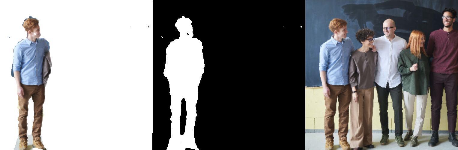
man with blonde hair in blue shirt and brown pants

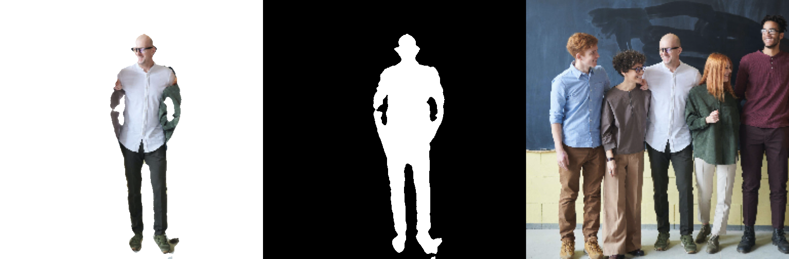
bald man wearing glasses with white shirt and black pants

Figure 1: Zero-Shot Segmentation with phrases: We highlight the ability of Peekaboo to ground complex language prompts onto an image with no segmentation specific training. An off-the-shelf diffusion model is used with only an inference time optimization technique to generate these segmentations. If you look closely, you’ll notice the bald man’s arms are segmented - but are not visible in the photo! Peekaboo has fairly strong shape priors.

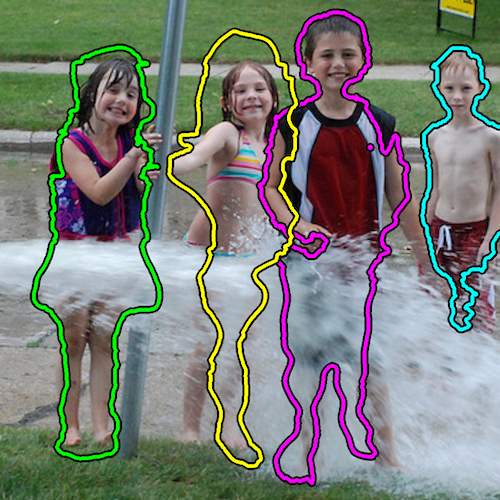
girl left in purple
boy in red vest
small girl with striped bikini
small shirtless boy on the right

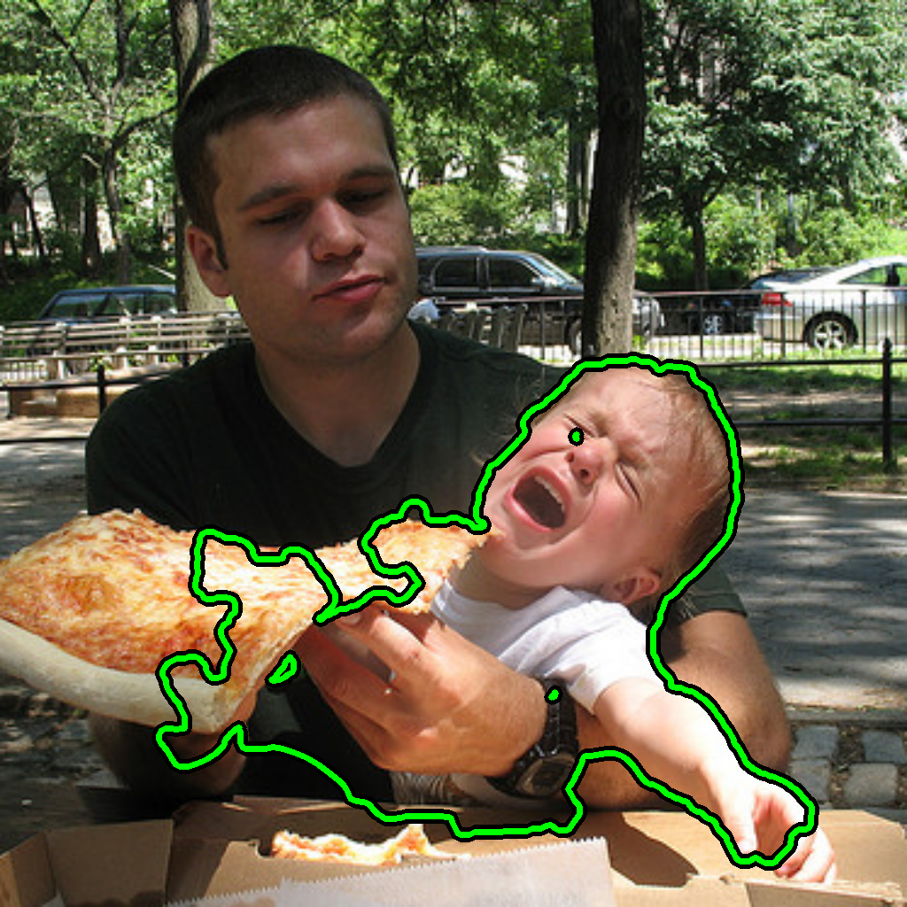
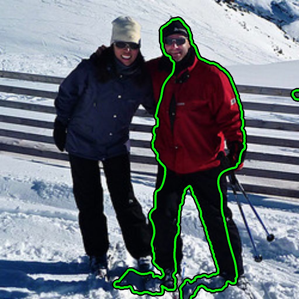
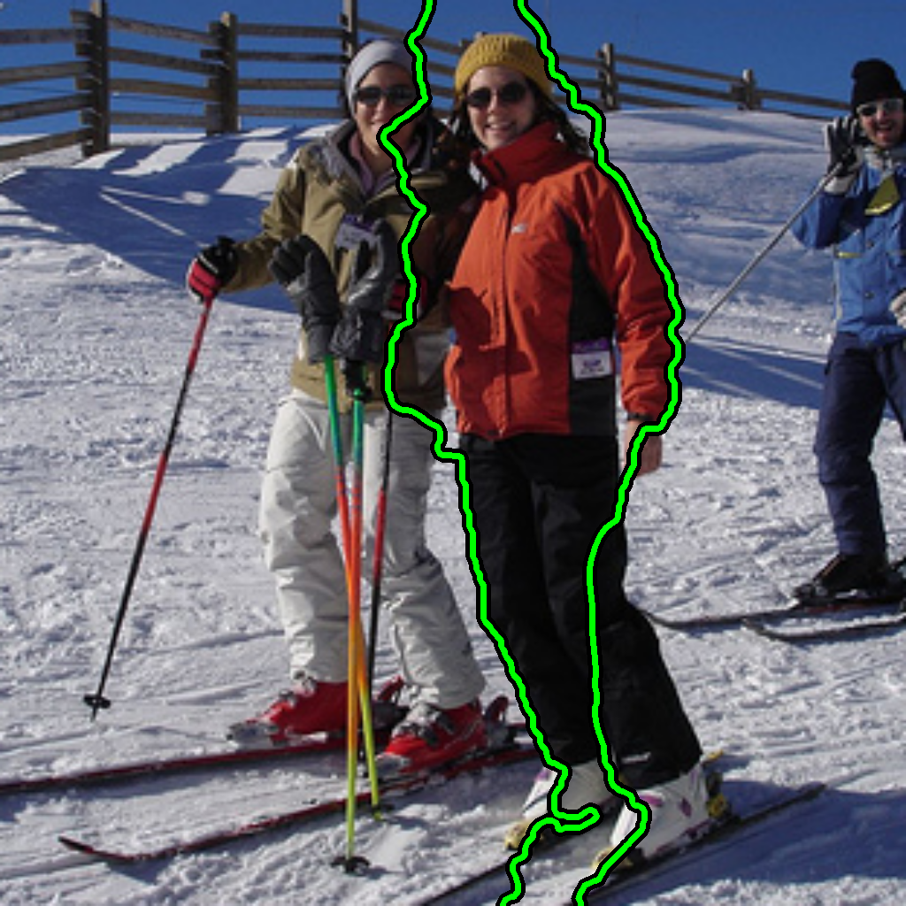
Figure 2: Peekaboo Samples: (left) we apply referring segmentation for each object in an example image from RefCOCO using custom text prompts listed below the image. (right) We illustrate 6 more examples from RefCOCO using their existing captions, listed left to right for top and bottom respectively: "baby", "brown cow", "elephant on right", "guy in red", "red jacket", "the front horse".

2 Related Work

Vision-Language Models: Vision-language models have advanced rapidly, enabling zero-shot image recognition [20, 21] and language generation from visual inputs [22, 23, 24, 25]. Recent contrastive language-image pre-training models [8, 9] showcase open-vocabulary and zero-shot capabilities, with extensions for a wide range of tasks [26, 27, 28, 29, 30, 31, 32, 33]. Grounding language to images [34, 6] and unsupervised segmentation [11, 12] have also been explored. Our proposed Peekaboo leverages an off-the-shelf diffusion model without segmentation-specific re-training and handles sophisticated compound phrases.

Diffusion Models: Diffusion Probabilistic Models [14] have been adopted for language-vision generative tasks [35, 36, 37, 38, 39, 40, 41] and extended to various applications [42, 43, 44, 45]. Recent works [45, 46] sample diffusion models through optimization. Our Peekaboo utilizes efficient latent diffusion models and is the first zero-shot method for cross-modal discriminative tasks such as segmentation.

Score Distillation Loss: SDL was introduced in DreamFusion [45] and applied to NeRF [47] to create 3D models. Our work applies it to alpha masks for image segmentation, yielding better results than previous CLIP-based techniques [48, 49, 50]. Like Peekaboo, SDL is also used with Stable Diffusion in [51, 52, 53].

Unsupervised Segmentation: Unsupervised segmentation [54] has evolved from early spatially-local affinity methods [55, 56, 57] to deep learning-based self-supervised approaches [58, 59, 60, 61, 62]. LSeg [7] is a semi-supervised segmentation algorithm because it’s trained with ground truth segmentation masks, but attempts to generalize the dataset labels to language using CLIP embeddings. Our Peekaboo also enables grouping aligned to natural language, is open-vocabulary.

Referring Segmentation: Referring segmentation [2, 63, 64] involves vision and language modalities. Early approaches [2, 65, 66, 67] fuse features, while recent works use attention mechanisms [68, 69, 64, 70, 71] and cross-modal pre-training [10]. Large supervised segmentation models [72, 73] have demonstrated high performance, but they require annotated segmentation datasets. Concurrently, an unsupervised referring segmentation method [16] has been developed using the same Stable Diffusion model as us, but it requires significant computational resources, including 5.3 days of training with 32 NVIDIA V100 GPUs. In contrast, Peekaboo is the first to perform unsupervised referring segmentation without necessitating any model training, effectively reducing the training time to 0 days on 0 GPUs.

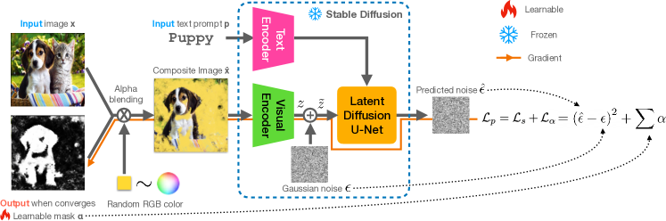
Figure 3: Overview of Peekaboo Architecture: We illustrate how an input image and random background are alpha blended to generate a composite image. This image and its relevant text prompt are processed by our diffusion model based inference-time objective. Iterative gradient based optimization of the randomly initialized alpha mask converges to a segmentation optimal for the conditioning text prompt. Note that our diagram shows the alpha mask at an intermediate iteration: at the initial iteration it is entirely random Gaussian noise.

3 Proposed Method

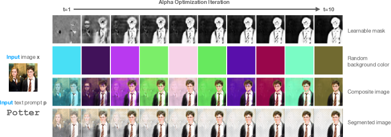
Figure 4: Inference Process: Above we show a timelapse of the inference-time alpha mask optimization process

In this section, we discuss our zero-training approach for unsupervised zero-shot segmentation, Peekaboo. We formulate segmentation as a foreground alpha mask optimization problem and leverage a text-to-image stable diffusion model pre-trained on large internet-scale data. The alpha mask is optimized with respect to image and text prompts.

3.1 Background: Score Distillation Sampling

First introduced in DreamFusion [45], Score Distillation Sampling (SDS) is a method that generates samples from a diffusion model by optimizing a loss function we call score distillation loss (SDL). This allows us to optimize samples in any parameter space, as long as we can map back to images in a differentiable manner. We modify SDS to optimize learnable alpha masks and operate with latent diffusion.

3.2 Overview

Consider an image of a puppy. Its defining region is the foreground (region containing the puppy): all distinctive characteristics of the puppy are retained even when the background is completely altered. Peekaboo leverages this idea to iteratively optimize a learnable alpha mask such that it converges to the optimal foreground segmentation. We use a randomly initialized alpha mask ($\boldsymbol{\alpha}$) to alpha-blend the puppy image ($\mathbf{x}$) with different backgrounds ($\mathbf{b}$), generating new composite images ($\hat{\mathbf{x}}$) as described in Eq. 1:

$$\hat{\mathbf{x}}=\boldsymbol{\alpha}\mathbf{x}+(1-\boldsymbol{\alpha})\mathbf{b}$$ (1)

The composite image and related text prompt ($\mathbf{p}$) are jointly processed by a pre-trained text-to-image diffusion model. An SDL based objective building off its output is minimized by iteratively optimizing the alpha mask. Minimizing this inference-time objective makes each new composite image similar to the text prompt (e.g. puppy) in latent space. We next discuss this inference-time objective in detail.

3.3 Inference-time Objective

Peekaboo’s inference-time objective $\mathcal{L}_{p}$ has two components: latent score distillation loss $\mathcal{L}_{s}$ and alpha regularization loss $\mathcal{L}_{\alpha}$. The total loss, $\mathcal{L}_{p}=\mathcal{L}_{s}+\mathcal{L}_{\alpha}$, is called the Peekaboo loss.

Latent Score Distillation Loss or $\mathcal{L}_{s}$ can be conceptually interpreted as a measurement of cross-modal similarity between a composite image and a text prompt $\mathbf{p}$. The key intuition lies in how predicted noise from the diffusion model is minimal for samples better matching the conditional distribution. Peekaboo utilizes Stable Diffusion that operates in a latent space. We adapt standard SDL to operate within this latent space, hence the term latent score distillation loss.

The Stable Diffusion model jointly processes images and text. Its visual encoder first projects images to a latent space. This latent vector is then processed by the diffusion U-Net ($\mathcal{D}$) conditioned on text embedding (from text encoder $\mathcal{T}$) to produce noise outputs. To measure $\mathcal{L}_{s}$, we first degrade latent vector $z$ of composite image $\mathbf{x}$ using forward diffusion, introducing Gaussian noise $\epsilon\sim\mathcal{N}$ to $z$, resulting in a noisy $\tilde{z}$. We then perform diffusion denoising conditioned on the text embedding with pre-trained $\mathcal{D}$. Our loss $\mathcal{L}_{s}$ is measured as the reconstruction error of noise $\epsilon$, given noisy $\tilde{z}$ and text embedding $\mathcal{T}\left(\mathbf{p}\right)$ as in Eq. 2:

$$\mathcal{L}_{s}=\mathrm{MSE}\left(\epsilon,\mathcal{D}\left(\tilde{z},\mathcal{T}\left(\mathbf{p}\right)\right)\right)$$ (2)

where MSE refers to mean-squared loss. Pseudo-code describing $\mathcal{L}_{s}$ in detail is presented in Algorithm 1.

Algorithm 1 Pytorch style pseudocode for Peekaboo

⬇

1import torch, stable_diffusion as sd

2

3def segment_image_via_peekaboo(img, prompt):

4 """Given␣an␣image␣and␣text␣prompt,␣return␣an␣alpha

5␣␣mask␣that␣is␣close␣to␣1␣in␣regions␣where␣prompt

6␣␣is␣relevant␣and␣0␣where␣the␣prompt␣is␣not."""

7

8 alpha = LearnableAlphaMask(img) # nn.Module

9 optim = torch.optim.SGD(alpha.parameters())

10

11 for _ in range(num_iterations):

12 peekaboo_loss(img, prompt, alpha()).backward()

13 optim.step() ; optim.zero_grad()

14 return alpha()

15

16def peekaboo_loss(img, prompt, alpha):

17 """Core␣of␣our␣paper.␣Blends␣image␣with␣random

18␣␣color␣and␣returns␣loss␣guiding␣alpha␣mask."""

19

20 img_embedding = sd.vae.encoder(img)

21

22 background = torch.random(3) # random RGB color

23 composite_img = torch.lerp(background, img, alpha)

24

25 loss = alpha_regularization_loss = alpha.sum()

26 loss += score_distill_loss(img_embedding, prompt)

27

28 return loss

29

30def score_distill_loss(image_embedding, prompt):

31 """Same␣loss␣proposed␣in␣DreamFusion"""

32 timestep = random_int(0, _diffusion_step)

33 noise = sd.get_noise(timestep)

34 noised_embed = \

35 sd.add_noise(image_embedding, noise, timestep)

36 with torch.no_grad():

37 text_embed = sd.clip.embed(prompt)

38 predicted_noise = \

39 sd.unet(noised_embed, text_embed, timestep)

40 return (torch.abs(noise - predicted_noise)).sum()

41

42class LearnableAlphaMask(nn.Module):

43 """This␣class␣parameterizes␣the␣alpha␣mask"""

44 def __init__(self, image):

45 _, H, W = image.shape

46 self.alpha = nn.Parameter(torch.random(1, H, W))

47 self.img = image

48 def forward(self):

49 alpha = bilateral_blur(self.alpha, self.img)

50 return torch.sigmoid(alpha)

Alpha Regularization Loss or $\mathcal{L}_{\alpha}$ enforces a minimal alpha mask. Specifically, $\mathcal{L}_{\alpha}=\sum_{i}\boldsymbol{\alpha}_{i}$, where $i$ indexes pixel location in $\boldsymbol{\alpha}$. Assuming a target is in our image, a trivial way to satisfy cross-modal similarity ($\mathcal{L}_{s}$) is to include all pixels. That is, setting $\boldsymbol{\alpha}=\mathbbm{1}^{H\times W}$ (all ones array). In this case, composite image $\hat{\mathbf{x}}$ would satisfy the prompt since $\hat{\mathbf{x}}$ is identical to input image $\mathbf{x}$. To combat this, we penalize high $\boldsymbol{\alpha}$ values with regularization, discouraging unnecessary pixels from being added.

3.4 Alpha Mask Parametrization

We next discuss the parametrization of our learnable alpha mask. Our experiments indicate that representing an alpha mask as a simple learnable matrix (referred as raster parametrization) yields sub-optimal results. To improve this, we apply a bilateral blur to that matrix and then clip it between 0 and 1 using a sigmoid function. This approach, defined raster bilateral parametrization, allows us to align our generated segmentation masks with the image content at a pixel level, respecting boundaries between regions present in the image. As a result, we are able to achieve better segmentation. We also investigate alternative parametrizations in section 3.4.1.

3.4.1 Peekaboo’s Bilateral Filter

In this subsection, we provide a detailed exploration of the bilateral filter, briefly introduced above.

A standard bilateral filter is a non-linear filter that smooths an image while preserving its edges. It does this by considering both the spatial distance and color differences between pixels, giving higher weight to pixels that are close in space and have similar colors.

We apply a modified version of this filter onto the learnable alpha mask. This filter operates on the alpha mask tensor and modifies it using the color and spatial information of the image to be segmented. This filter is applied at every step the alpha optimization process, as opposed to during post-processing.

The intention behind using such a filter is to ensure that our generated segmentation masks adhere to the image content at a pixel level from early iterations, leading to improved segmentation in the end.

In this section, we present results, both quantitative and qualitative for our downstream tasks of segmentation. We first go over peekaboo and our baseline algorithms, then talk about the specific experiments.

3.5 Baselines

Following [2], we build a baseline that predicts the entire image as the segmentation tagged Random (whole image). For our next baseline, we apply the weakly-supervised segmentation method GroupViT [11]. Note that GroupViT is intended for text conditioned segmentation and is trained on datasets similar to those used by Stable Diffusion (i.e. our off-the-shelf diffusion model). Our last baseline, LSeg [66] is a semi-supervised segmentation alogorithm that has seen the VOC dataset during its training.

3.6 Peekaboo Variants

We our experiments we showcase several different variants and ablations of Peekaboo. Fig. 5 gives a qualitative comparison between these variants.

“RGB Bilateral” is the main, default Peekaboo algorithm described in Section 3. For more details on these methods, please see the appendix. “CLIP”: this variant substitutes score distillation loss for a CLIP-based [8] loss similar to [49]. All of the other variants are changes solely to the alpha mask parametrization. “Raster”: this ablation skips the bilateral filter, and thus optimizes the alpha map pixel-wise. This yields worse performance than any other parametrization. “Fourier”: this variant parametrizes the alpha mask with a fourier feature network [74], inspired by neural neural textures in [75]. This variant does not use a bilateral filter, but yields better results than a basic matrix parametrization. It tends to suffer from hallucinations more than other variants. “Fourier Bilateral”: Just like the Fourier variant, except with the bilateral filter on top. This yields higher performance than the fourier feature network alone. “Depth Bilateral”: Uses a depth map generated using the off-the-shelf monocular depth estimation model MIDAS [76] to guide the bilateral filter instead of differing RGB values. Intuitively, it means that pixels that are close in 3d space will have similar alpha values. This variant performs better than the main Peekaboo algorithm, and outperforms Clippy [12] on both COCO and VOC-C.

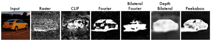
Figure 5: Visual Variant Comparison: This figure gives qualitative comparisons between Peekaboo variants on a single image from VOC-C with the prompt “car”.

4 Experiments

4.1 Referring Segmentation

We first present our quantitative evaluations for referring segmentation in Tab. 1. These results presented in Tab. 1 showcase impressive performance of Peekaboo.

The RefCOCO dataset is farily challenging, as the prompts are complex refer to a specific portion of the image. Some example prompts: “giant metal creature with shiny red eyes”, “bartender at center in gray shirt and blue jeans”, and “suitcase behind the zebra bag”.

GroupViT is a key comparison to our work, given how it is trained on similar noisy image-caption pair from internet scraped data. And on this dataset, Peekaboo outperforms GroupViT - a model that was trained specifically for segmentation on 16 NVIDIA V100 GPUs for two days. LSeg was trained for segmentation and outperforms Peekaboo, but we would like to reiterate - Peekaboo simply utilizes a diffusion model originally trained for text-to-image generation, and adopts it to segmentation with no re-training.

4.2 Semantic Segmentation

Type	Method	Prec@0.2	Prec@0.4	Prec@0.6	Prec@0.8	mIoU
Baselines	Random	.141	.022	.003	.000	.102
	GroupVIT [11]	.212	.075	.020	.002	.112
	LSeg [7]	.512	.212	.051	.008	.235
Peekaboo Variants (ours)	Depth Bilateral	.359	.135	.037	.003	.204
	RGB Bilateral	.318	.099	.018	.002	.163

Table 1: Referring Segmentation Evaluation. We present results on the RefCOCO dataset. Numbers reported are precision and mIoU values for our method and baselines. Once more, unlike the others, Peekaboo is without any segmentation training.

Type	Method	Prec@0.2	Prec@0.4	Prec@0.6	Prec@0.8	mIoU
Baselines	Random	.670	.198	.032	.012	.281
	Clippy [12]	.757	.459	.263	.049	.539
	GroupViT [11]	.862	.778	.602	.205	.578
	LSeg [7]	.952	.897	.758	.311	.678
Peekaboo Variants (ours)	Raster	.756	.323	.103	.012	.340
	CLIP	.918	.488	.093	.023	.430
	Fourier	.862	.598	.231	.084	.454
	Bilateral Fourier	.845	.608	.281	.123	.470
	Depth Bilateral	.929	.707	.455	.187	.551
	RGB Bilateral	.892	.709	.331	.130	.520

Table 2: VOC-C Semantic Segmentation Evaluation. Our results on the VOC-C dataset report mIoU values for our method and GroupViT baseline. Numbers for our baselines are obtained running their respective pre-trained models. Numbers reported are precision and mean-IoU values.

We present evaluations on the VOC-C dataset in Tab. 2. Our modified Pascal VOC dataset, VOC-C, was created by selecting and cropping images from the original VOC2012 dataset with single subjects larger than 128x128 pixels.

The text prompts VOC-C dataset relatively simple. They’re simply the names of the dataset’s 20 classes. Some examples: “cat”, “dog”, “aeroplane”, “bird” - etc.

While Peekaboo doesn’t outperform Clippy, GroupViT or LSeg, it has fairly competitive performance. In fact, Peekaboo’s “Depth Bilateral” variant even outperforms Clippy. And to reiterate, unlike these baselines, Peekaboo requires no training whatsoever.

4.3 Qualitative Results

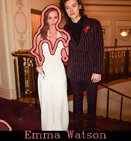
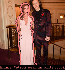
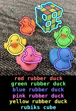
Figure 6: Varying granularity (left): Another feature of Peekaboo is its ability to segment at differing granularity. While the model performance in such situations is quite sensitive to the caption, we highlight how subtle variations to the caption allows us to localize relevant regions of image accordingly. Real-world applications (right): Peekaboo can localize real-world objects from arbitrary captions. We highlight how each localization successfully captures the relevant region with a clear overlap over each object centroid. This is particularly useful in applications such as robotics where interaction with arbitrary objects defined by natural language can be valuable.

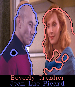
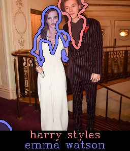
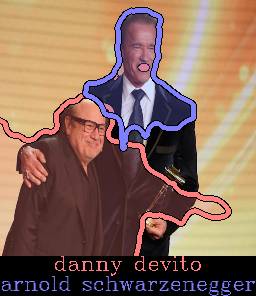
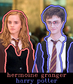
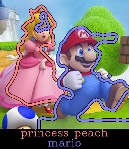
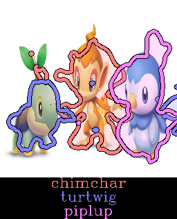
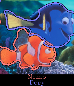
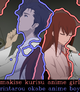
Figure 7: Peekaboo is truly open vocabulary: We illustrate examples where Peekaboo is able to localize various regions of interest defined by references from popular culture. All of these are examples where the model has been able to correctly localize (identified region centroid or high IoU with correct region). The caption below each image is used to generate the same color mask. An interesting behavior of our model is its localization to the region most defined by the accompanying text caption. For example, in the case of Emma Watson in the top row second figure, it is visible how Peekaboo localizes on her face and body instead of her frock (see Fig. 6 for more on this).

In this section, we present some more qualitative evaluations of our proposed method. In Fig. 7, we show some randomly selected examples where Peekaboo successfully localizes regions of interest based on popular cultural references. We hypothesize that our Peekaboo is able to understand such a wide vocabulary due to the strength of the pre-trained diffusion model, which was trained on an interet-scale dataset. We also analyze real-world image captured by our camera in Fig. 7.

Another characteristic of this open vocabulary nature that endows our model is to probe image regions at varying granularities. We illustrate this behavior in Fig. 6 where sub-regions of a single person can be localized based on different text captions.

5 Generating Images with Transparency

Peekaboo loss can do more than just segment images - it can generate images with transparency. In fact, it does this quite reliably - giving detailed alpha masks along with each generated image. Images with transparency are incredibly useful for many domains, such as graphic design assets and video game textures. However, to the best of our knowledge, all current text-to-image models such as [38][77][40][37] have trained strictly on RGB images, and are not designed to generate images with an alpha channel.

Despite the absence of such models, we can generate RGBA images by iteratively optimizing an RGB image jointly with an alpha mask using Peekaboo loss. Pseudocode for this process is given in Algorithm 2, which builds on Algorithm 1.

Algorithm 2 Pytorch style pseudocode for transparent RGBA image generation

⬇

1 #Continued from Algorithm 1

2 def text_to_rgba_image(prompt):

3 """Given␣a␣text␣prompt,␣generate␣a␣new␣RGBA␣image

4␣␣␣␣␣␣␣␣(An␣image␣with␣an␣alpha␣transparency␣mask)"""

5

6 alpha = LearnableAlphaMask() # nn.Module

7 image = LearnableRGBImage() # nn.Module

8 optim = torch.optim.SGD(alpha.parameters(), image.parameters())

9

10 for _ in range(num_iterations):

11 peekaboo_loss(image(), prompt, alpha()).backward()

12 optim.step() ; optim.zero_grad()

13 return image(), alpha()

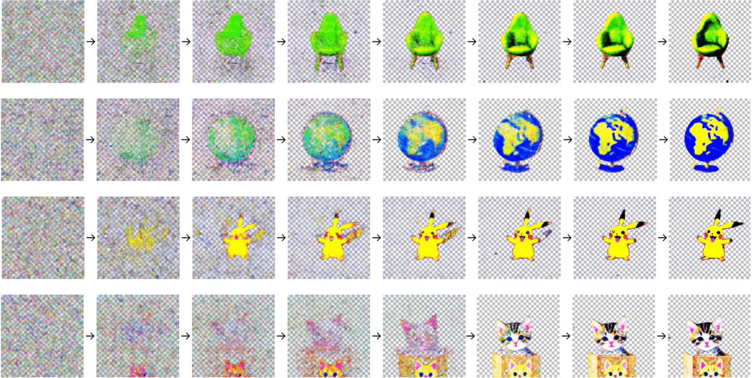
Figure 8: Image Generation Timelapse: Above we show a timelapse of the RGBA image generation process. The prompts from top to bottom are “avocado armchair”, “globe”, “pikachu”, “cat in a box”. More examples are in the appendix. The images are on checkerboards to illustrate transparency.

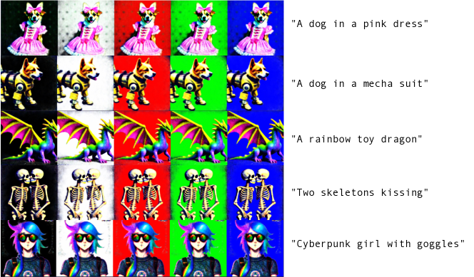
Figure 9: Image Generation Examples: Above we show five more examples of RGBA images generated with this method, placed on different backgrounds. Note how Peekaboo successfully separates high-frequency details, for example, between rib bones and the background.

Example images can be found in Fig. 9 and Fig. 8.

This process of creating images via optimization is very similar to [51], which also uses score distillation loss to optimize 2d images. However, it also suffers from some of the same caveats.

6 Conclusion

In this work, we established how text-to-image diffusion models trained on large-scale internet data contain strong cues on localization. Note that their training process contains no explicit modelling of localization. We then propose a novel inference-time optimization technique that can extract this localization knowledge and apply this to downstream referring and semantic segmentation tasks. In particular, we perform such segmentation with no segmentation-specific re-training of the diffusion modell, leaving its weights (and therein all strengths of the model) intact.

The major limitation of our work is its reliance on a large diffusion model pre-trained on internet-scale data. Given the difficulty of training such diffusion models under usual academic settings (resource constraints), approaches building off Peekaboo must rely on publicly available diffusion models. Moreover, all flaws and biases contained within such diffusion models [78] as well as internet-scale datasets used for training [79] will be transferred to Peekaboo.

Peekaboo: Text to Image Diffusion Models are Zero-Shot Segmentors

Appendix A Intuition

In this section, we aim to convey some intuition behind Peekaboo. We explore the reasoning behind each component used and explain why Peekaboo works as it does. The key underlying idea is deriving gradients from a conditional diffusion model to guide a mask generation process.

The diffusion model conditioned on a text caption processes a noisy input to generate a gradient that moves the input toward the target image. This gradient is what we use to guide our learnable alpha mask. We use Stable Diffusion [17], a text-to-image diffusion model trained on billions of internet images. This means the model will target to generate images from that image distribution relevant to a text caption. The noisy input is the image to be segmented alpha blended with a uniform background. Iteratively, it will attempt to update this input to a target distribution image relevant to the text caption. Updating the regions of the image most relevant to the text caption makes more sense. Thus, regions of the image relevant to this text caption will have stronger gradients than regions irrelevant to a prompt. For example, consider an image of a dog sitting on a couch. When prompted for “a dog”, the couch is irrelevant to the prompt and has fewer gradients focused on that region. There is less incentive to remove the alpha mask in that location, and without incentive, it defaults to null due to our alpha regularization loss (Algorithm 1). This results in the alpha mask focusing on the dog region.

While this results in our desirable behavior, we observe that it converges to the region most relevant to the text prompt. For example in Fig. 6, in segmenting Emma Watson, it attempts to focus on the region that mostly makes the image look like her, which could be a sub-portion of the human region (in accordance with the accepted notion of segmenting a human). While Harry Styles could wear a dress, he would still remain Harry Styles. However, only Emma Watson can have her face. Therefore, Emma Watson’s face is more essential to the prompt Emma Watson; hence it prioritized segmenting that region while ignoring the dress. In a way, one could view this as a new definition of segmentation; Peekaboo localizes the essence of an object described by language.

Appendix B Ablations

In this section, we present some ablations on components of our inference time optimization.

B.1 Alpha Regularization

The alpha regularization term $\mathcal{L}_{\alpha}$ (see Sec. 3.3) is important, because it prevents Peekaboo from including irrelevant parts of the image in the alpha mask. By adding this alpha penalty, we effectively tell Peekaboo to create a minimal alpha mask. In practice, the $\mathcal{L}_{\alpha}$ term should be scaled by a constant, which in our experiments was $\lambda_{\alpha}=.05$ (the alpha regularization coefficient).

In this section, we perform ablations where we vary this $\lambda_{\alpha}$ term. We play around with the alpha regularization coefficient $\lambda_{\alpha}$, scaling it by different factors. For example, “2x” means a $\lambda_{\alpha}$ that is “2x” the normal value, which is $.05\times 2=.1$.

We can view the results visually in both the transparent image generation and segmentation contexts. In the transparent image generation task Fig. 10, we see that the generated images are more transparent when $\lambda_{\alpha}$ is large. Likewise, in the segmentation task Fig. 11 we can see that Peekaboo generates smaller masks when $\lambda_{\alpha}$ is high.

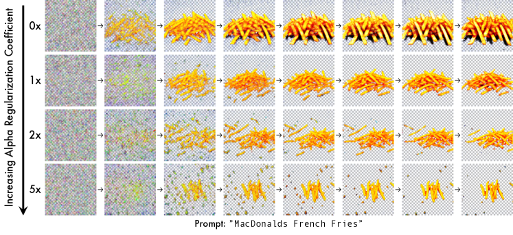
Figure 10: We display four transparent-image generation timelapses for the prompt “MacDonalds French Fries” with varying amonuts of alpha regularization. As we increase alpha regularization, Peekaboo tends to generate images with less alpha. In this case, it means less french fries will be generated. Conversely, when the $\lambda_{\alpha}$ is eliminated (aka $\lambda_{\alpha}=0$), more french fries than normal are generated.

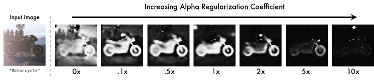
Figure 11: The alpha regularization term plays a large role when using Peekaboo to segment images. If $\lambda_{\alpha}$ is too large (on the far right), the entire image might be ignored. Conversely, if $\lambda_{\alpha}$ is too small, tons of background details are included.

B.2 Implicit neural representations

$\overrightarrow{\texttt{Iteration}}$

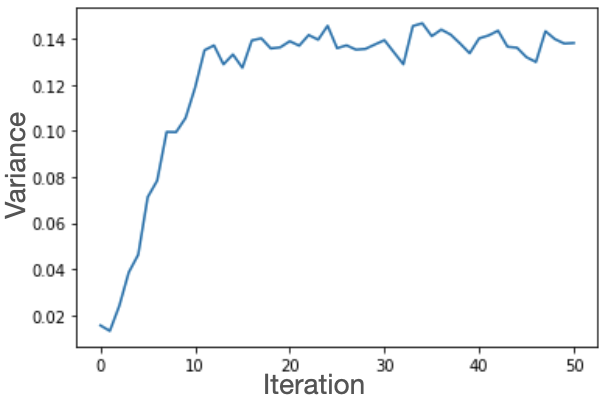
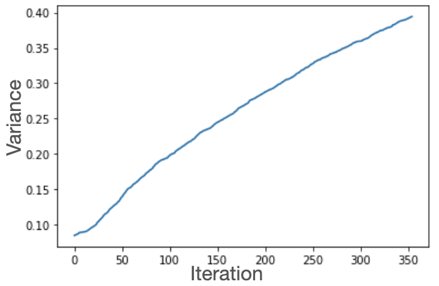
Figure 12: Ablation on implicit neural representation: In Peekaboo’s “Fourier” and “Bilateral Fourier” variants, as well as our transparency image generations, we utilize neural-neural textures [75], which use Fourier feature networks [80]. Here we compare against the alternative of direct pixel-level representations for RGB image generation. (top) The first row shows images generated using implicit representations while the second row shows those of pixel-level ones. The two graphs below correspond to pixel variance (y-axis) plotted against iteration (x-axis) for implicit and pixel-level representation respectively from left to right.

$\overrightarrow{\texttt{Iteration}}$

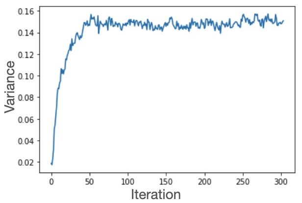
Figure 13: Visualizing implicit neural representation: We illustrate another example of generating an image using our implicit neural representation (top) vs pixel-wise representation (bottom). To the left we show a graph of pixel level variance (y-axis) plotted against iteration (x-axis) for the implicit representation case. In this example, we highlight how the characteristics of the cat (shape, location) is consistent in the pixel-wise case from early iterations. However, in our implicit (parametric) representation, various characteristics of the cat (e.g. size, position) alter throughout the iterations. This latter kind of behaviour is also favourable to our task of mask generation.

In Peekaboo’s “Fourier” and “Bilateral Fourier” variants, as well as our transparent image generations, we use the neural-neural texture formulation from [75] to represent our learnable alpha masks (and RGB channels in transparent image generations, and foreground/background in our analogous example in Appendix E). The alternative to using this implicit neural representation is learning the pixels directly by representing them as a learnable tensor of dimensions $(H,W,C)$ for $C=1$ in mask and $C=3$ in RGB images. In this ablation, we explore how the alternative compares against our selected approach. We highlight the two main drawbacks of pixel-level representations as 1) noisy outputs and 2) bad convergence.

We illustrate this behavior in Fig. 12. First, we attempt to generate images using each of the two image parametrizations through score distillation sampling. We show that neural representations lead to less noisy outputs. The top two rows in Fig. 12 correspond to these. Clearly, the neural representation in the first row leads to a less noisy output in comparison to the alternative. Next, we explore the convergence behavior of each approach. To analyze this, we utilize the images being generated and measure their variance at the pixel level. While a natural image contains some variance in pixel space, this is a finite value, and our run-time optimization should ideally converge at this variance. However, utilizing a pixel-level representation results in continuously increasing variance in the image pixels, leading to overly saturated images (dissimilar to a realistic image) and in the case of masks, lack of convergence. This is illustrated in the two graphs at the bottom of Fig. 12. We also highlight how in these graphs of Fig. 12 the variance of the implicit representation converges early on at around 50 iterations (left) while that of the pixel-wise representation (right) fails to converge even after 350 iterations.

B.3 Bilateral Filter

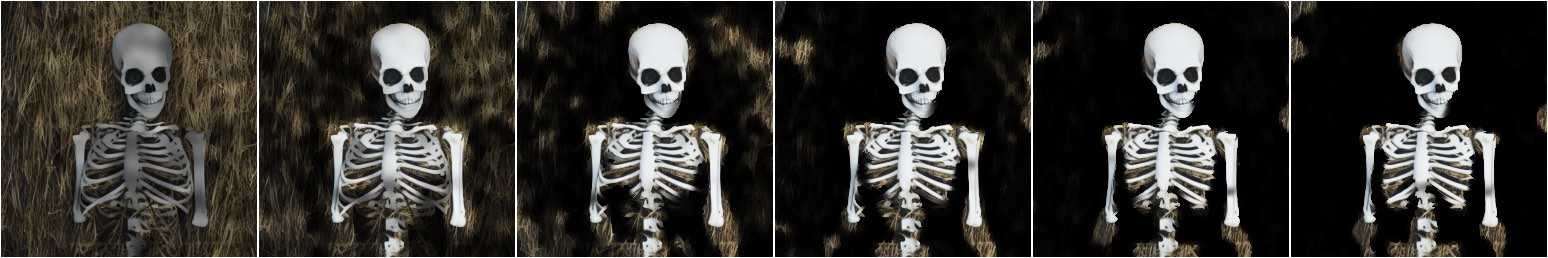
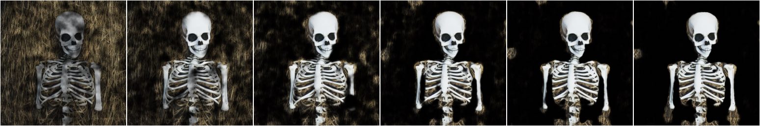
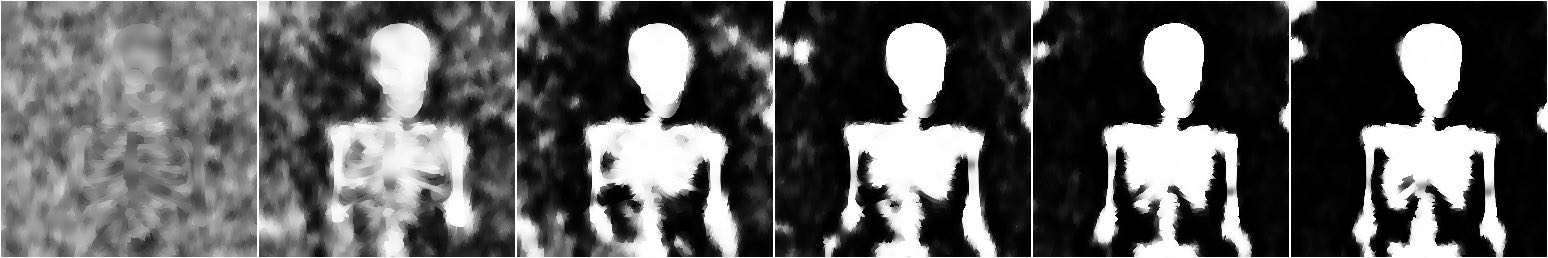
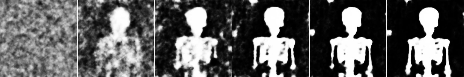
$\overrightarrow{\texttt{Iteration}}$

Figure 14: Ablation on bilateral filters: The bilateral filter improves segmentation alignment with object boundaries, resulting in more accurate and precise segmentations. In this figure, we show a timelapse of the alpha mask optimization process over time from left to right, for both Peekaboo variants “Fourier” and “Bilateral Fourier” (see Sec. 3.4.1). The bottom two rows show a timelapse of the alpha maps, and the top two rows show a timelapse of those alpha maps overlaid on the original image to help visualize their accuracy. The first and third rows depict the “Fourier” variant, while the second and fourth rows depict the “Bilateral Fourier” variant.

In Sec. 3.4.1, we discussed Peekaboo’s use of a bilateral filter as part of the image parametrization. In this section, we provide a visualization of this filter. A closer look at the noisy mask in row 3 column 1 of Fig. 14 will show vague outlines of a skeleton within the noise; this is a result of the modified bilateral filter being applied to the mask.

Appendix C Optimization Details

In this section, we discuss all details relevant to our proposed inference time optimization that generates segmentations. In order to generate a single segmentation, we run it for 200 iterations, a learning rate of $1e-5$, and stochastic gradient descent as the optimizer.

Additionally, we apply the modified bilateral blur operation, conditioned on the image to be segmented, onto the learnable alpha masks at initialization, which results in faster and better convergence. Here we use a blur kernel of size 3 with 40 iterations (multiple iterations increase the effective field of view for a kernel).

Appendix D Limitations

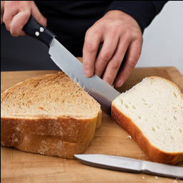
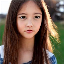
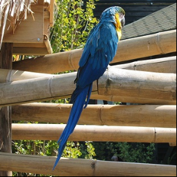
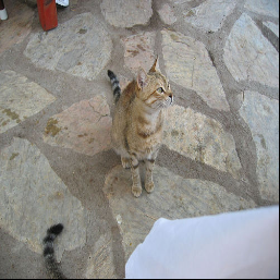
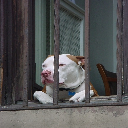
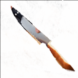
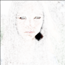
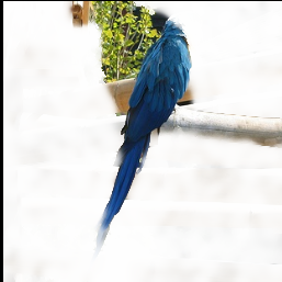
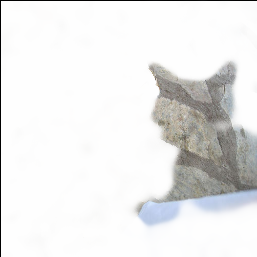
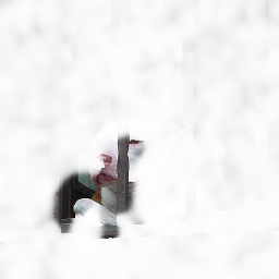
Figure 15: Limitations and failures of Peekaboo: We illustrate examples where Peekaboo fails to properly segment the region of interest. The prompts for these examples from left to right are: knife, eyes, bird, cat, dog. We note how a major issue is the tendency of Peekaboo to hallucinate the shape of the object denoted by the text caption.

We also acknowledge that our proposed Peekaboo contains various limitations and shortcomings. A key drawback is its failure cases that result in a hallucination of the text prompt using some random background region, i.e. it uses the background texture to create a region shaped like the underlying object described by the text. We illustrate this behavior in Fig. 15. This is clearly visible in the three right-most examples (bird, cat, dog). We also note that such behavior is more common when a simple (often one word) text caption is used. Another failure is the addition of unnecessary parts to the region of interest. For example, in column one of Fig. 15, while the knife is coarsely localized, Peekaboo also incorrectly creates a handle for it using a slice of bread from the background. The model also sometimes fails to converge entirely, as illustrated in the second column, where despite localizing the eyes, the generated mask also holds onto outlines of the image foreground object.

While we hope to address these issues in future work, we also reiterate that despite these limitations, Peekaboo is a first unsupervised method that is able to perform open vocabulary segmentation using arbitrary natural language prompts.

Appendix E Analagous Example

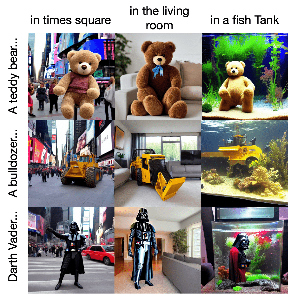
Figure 16: Images generated from Stable Diffusion: This data distribution is quite different from the distribution of natural images, rarely containing objects in non-central locations of the image. This bias is carried through to Peekaboo, which is why Peekaboo is best at segmenting objects near the center of an image. These images were generated by running prompts through stable diffusion v1.4, such as “a teddy bear in times square”, and using DDPM with a guidance scale of 7.

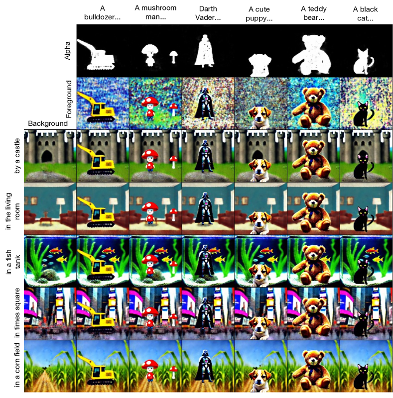
Figure 17: Can diffusion models separate foreground and background? Stable diffusion was only trained on RGB images. However, observing the often clean boundaries between objects in generated images, it begs the question: can we use these boundaries to generate images with transparency? In this figure, we conduct a self-contained experiment that answers this question: yes. We overlay 6 learnable foreground images on top of 5 learnable background images using 6 learnable alpha masks, to get a total of 30 learnable composite images. Each of these composite images has a composite caption, created by combining the foreground prompt with the background prompt. For example, the image created by combining background #1 and foreground #1 is accompanied by the prompt "a bulldozer by a castle". We optimize each of these 30 composite cells with score distillation loss (see Sec. 3.1) until each foreground, background and alpha mask has been learned. Differences between this experiment and Peekaboo are minimal: in Peekaboo, we only optimize the alpha masks, whereas in this analogous experiment we optimize everything.

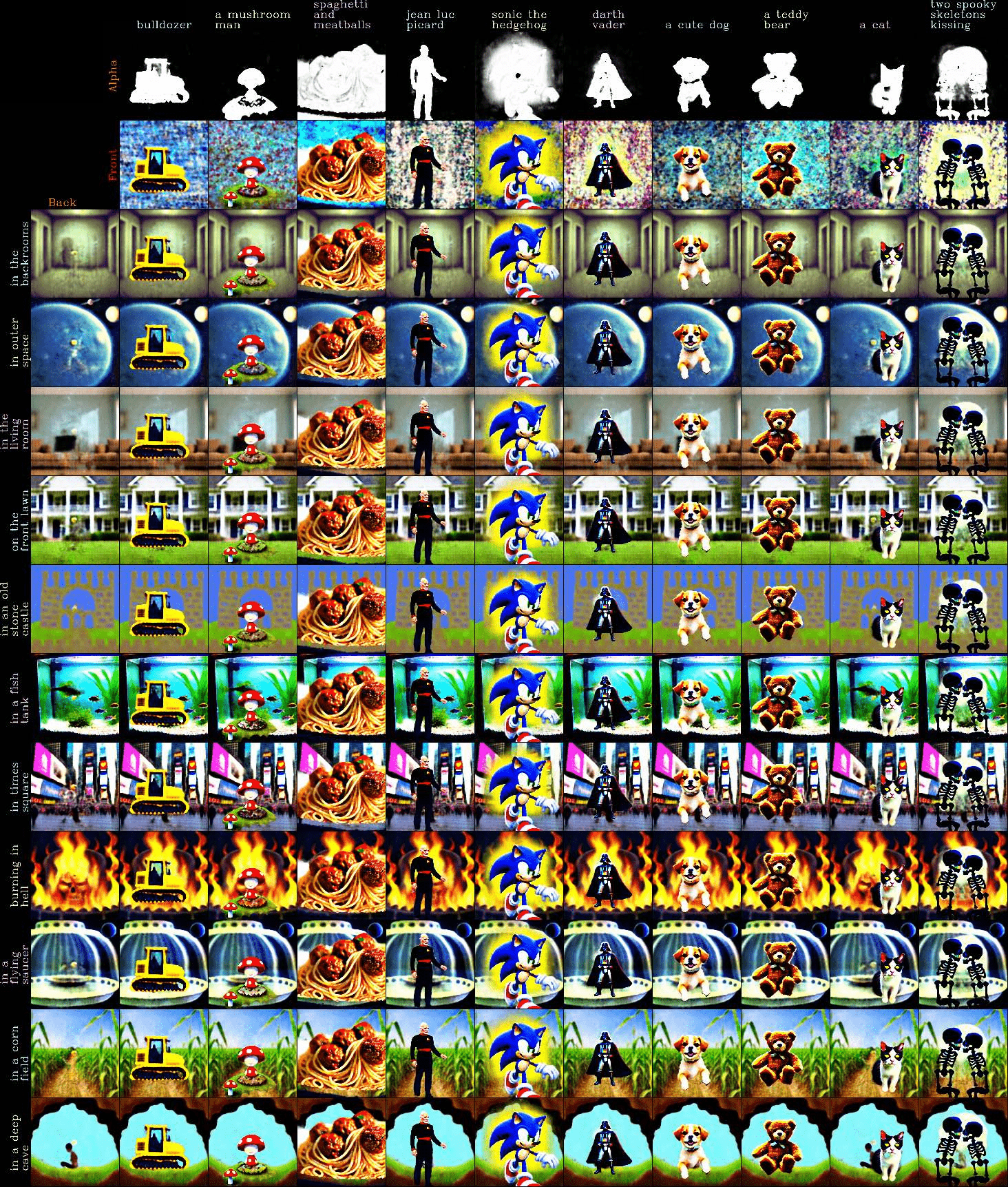
Figure 18: Extended visualization of analogous experiment

In order to explain the intuition behind Peekaboo, we show results of analogous experiment that helped to inspire it. This analagous algorithm is not exactly Peekaboo, but it is very similar and is helps explain the main idea behind how Peekaboo works.

We first examine a stable diffusion model [17] pre-trained on LAION-5B [81]. Our goal is to explore whether internal knowledge of these models regarding boundaries and localization of individual objects can be accessed and subsequently utilized for tasks such as segmentation. We focus on the case of generating a single synthetic object in some background and attempt to generate an accompanying alpha mask that demarcates the region belonging to the foreground object. We utilize score distillation loss (see Sec. 3.1) as a cross-modal similarity function that connects a text caption describing a foreground object to the image region it is located. Using this similarity as an optimization objective, we generate the foreground, background, and alpha mask.

Results obtained from this process are illustrated in Fig. 17. While our method is able to generate good segmentation masks relevant to the foreground, we note that generated images are unrealistic.

We highlight that generated image quality is indifferent to the segmentation component, where we generate single-channel alpha masks. The rest of our work is focused on how this technique can be leveraged for segmenting stand-alone images, i.e. images beyond those generated by a diffusion model. In essence, we attempt to segment real-world images with free-form text captions.

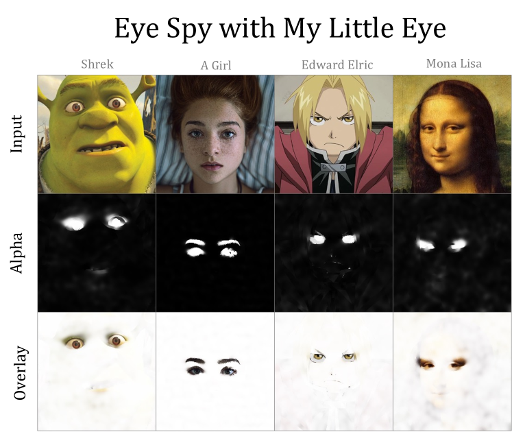
Figure 19: In this figure, we play a game: find the eyes! Peekaboo can segment specific features of images, and is good at finding eyes. Only one prompt was used: eyes. On the top row we have input images, and in the middle row we have the outputted alpha map. On the bottom we overlay the input images with a white mask corresponding to the alpha, to better show which part of the image it chose to segment.

Appendix F More Results

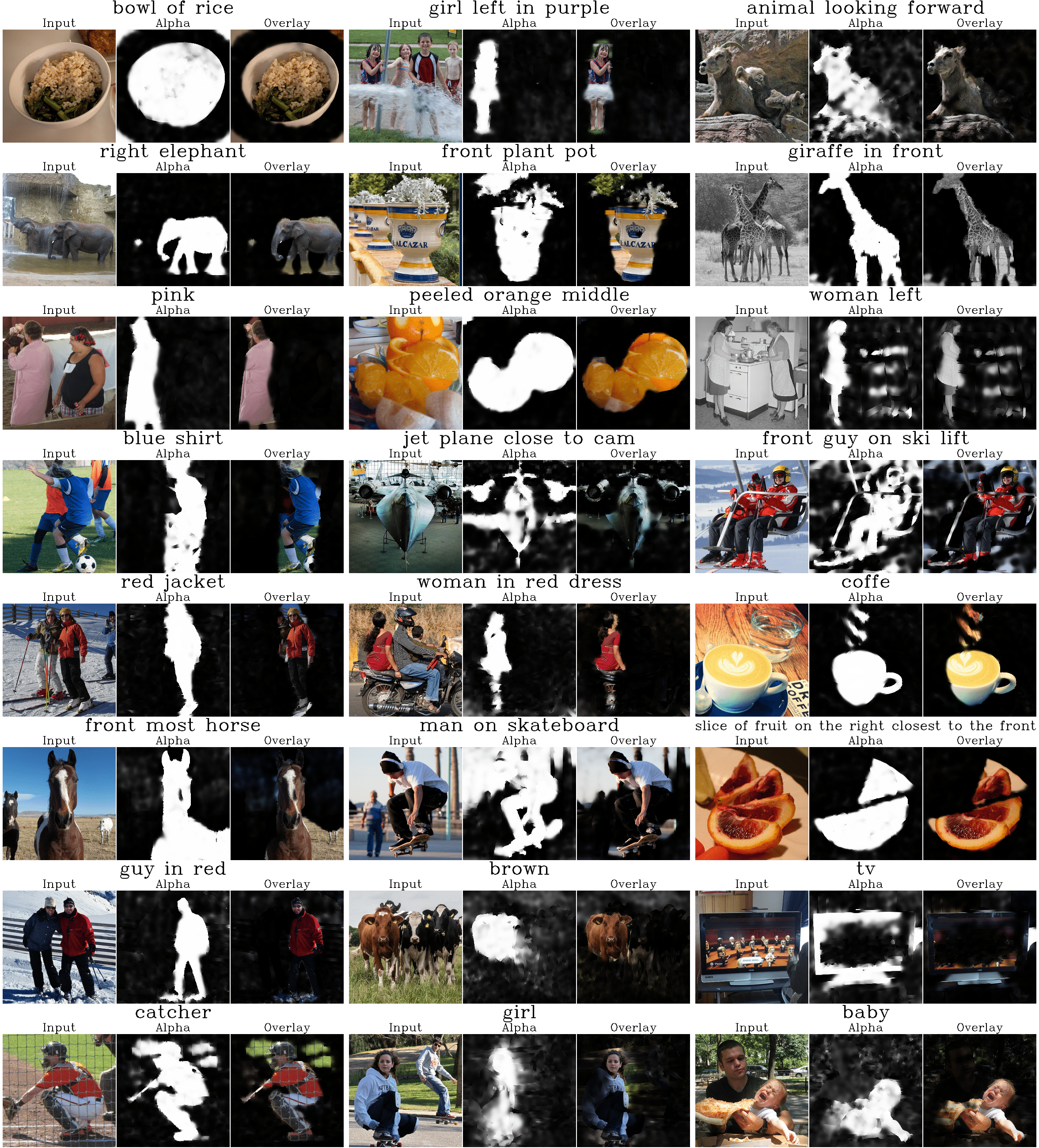
Figure 20: Our results on RefCOCO-C. For each sample we demonstrate the prompt text(title), input image(left), our output alpha mask(middle), and the image segmented by the mask(right)

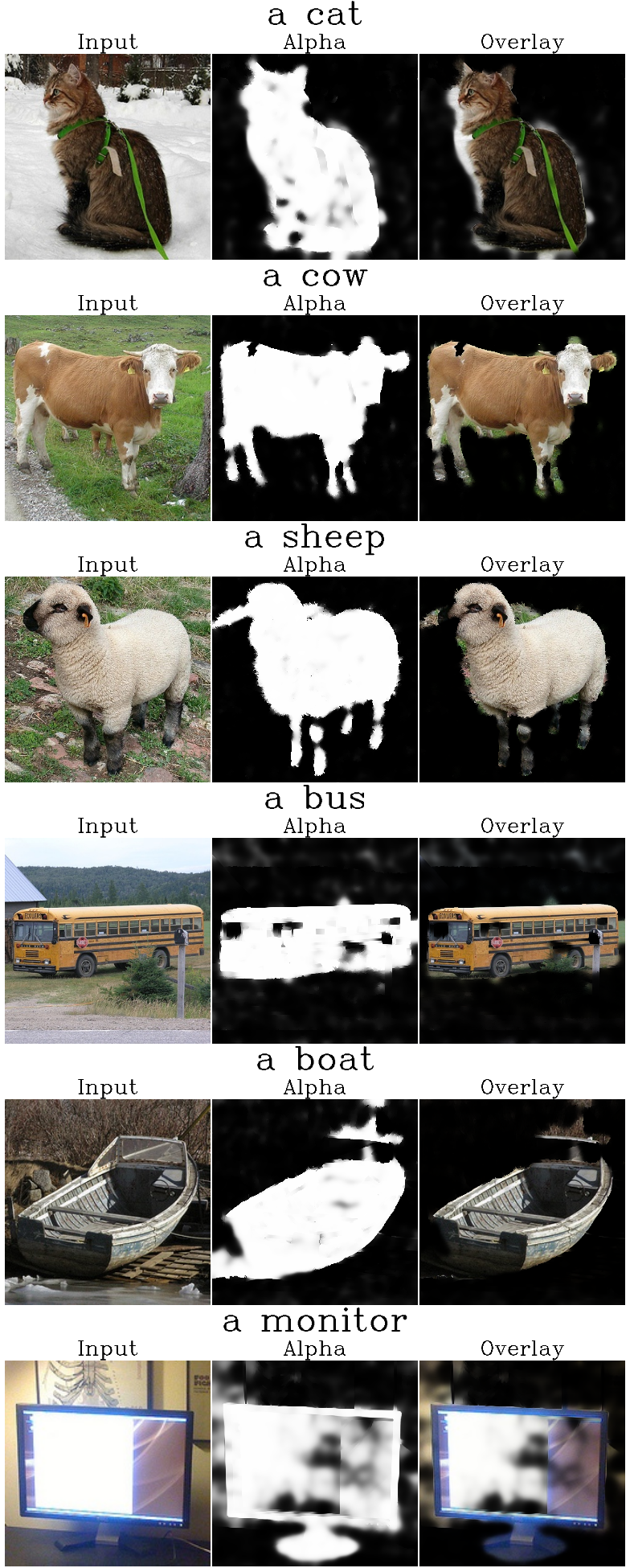
Figure 21: Our results on Pascal VOC-C. For each sample we demonstrate the prompt text(title), input image(left), our output alpha mask(middle), and the image segmented by the mask(right)

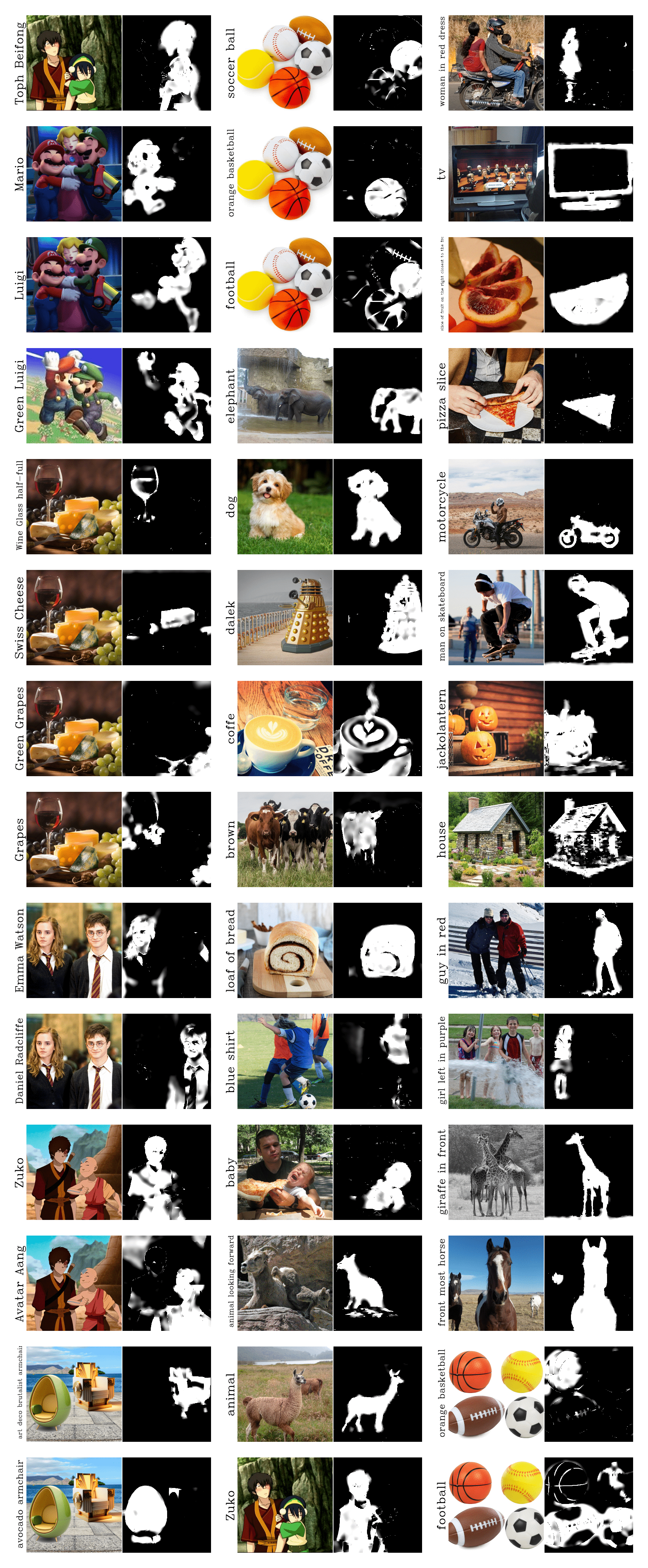
Figure 22: Peekaboo’s segmentation results on various images, including pop references such as Avatar the Last Airbender and AI-generated images of imaginary objects that don’t exist such as avocado armchairs. Prompt and input image are on the left, and the alpha mask output is on the right.

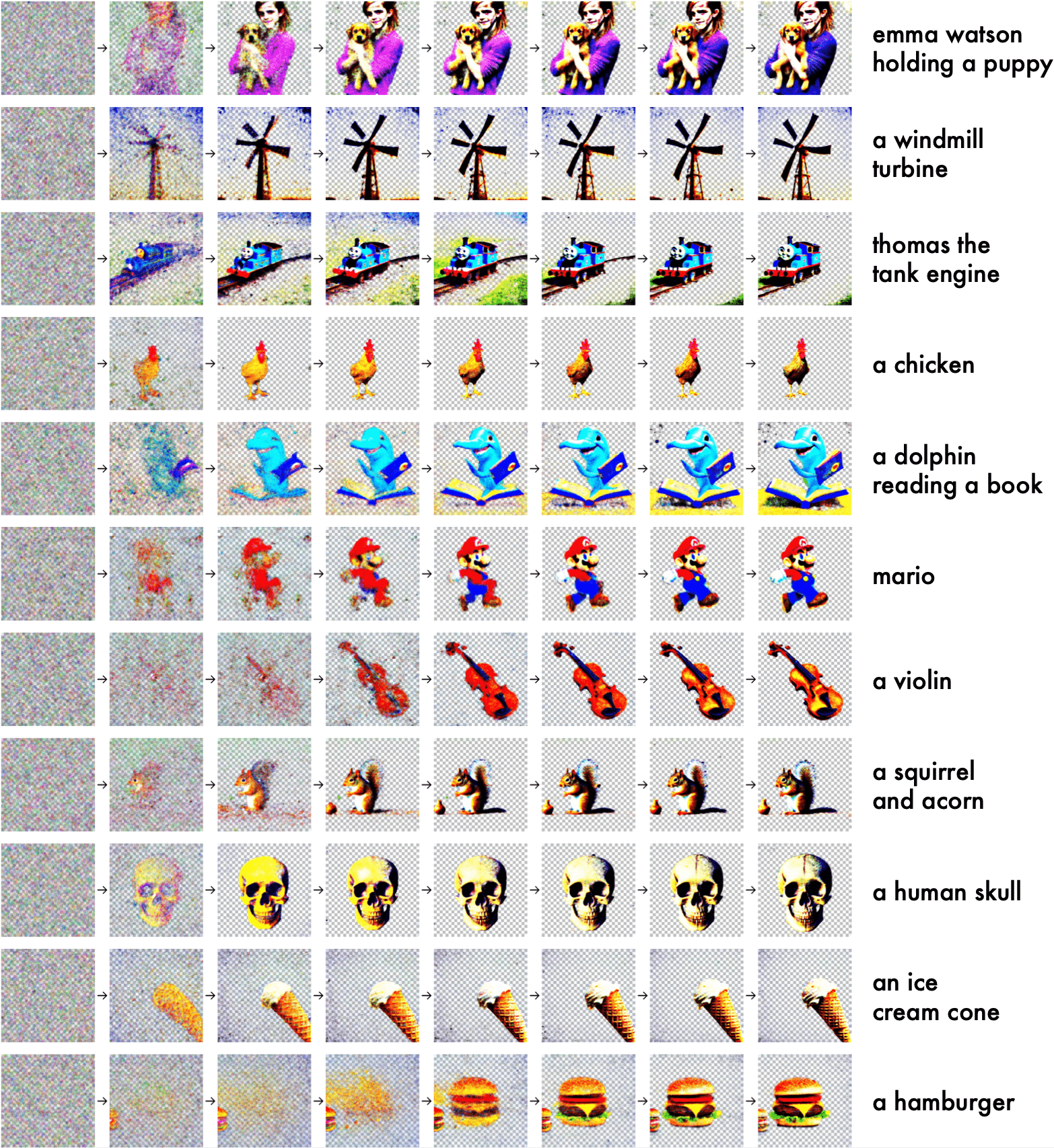
Figure 23: Part 1/2. Peekaboo can generate images with transparency masks! Continuing from Fig. 9, we display timelapses of the transparent image generation task described in Sec. 5. The prompt for each image is to its right.

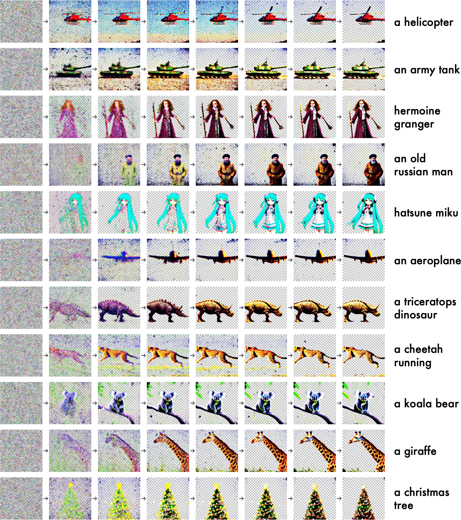
Figure 24: Part 2/2. Peekaboo can generate images with transparency masks! Continuing from Fig. 9, we display timelapses of the transparent image generation task described in Sec. 5. The prompt for each image is to its right.

References

- [1] Tsung-Yi Lin, Michael Maire, Serge Belongie, James Hays, Pietro Perona, Deva Ramanan, Piotr Dollár, and C Lawrence Zitnick. Microsoft coco: Common objects in context. In ECCV, 2014.
- [2] Ronghang Hu, Marcus Rohrbach, and Trevor Darrell. Segmentation from natural language expressions. In ECCV, 2016.
- [3] Pei Sun, Henrik Kretzschmar, Xerxes Dotiwalla, Aurelien Chouard, Vijaysai Patnaik, Paul Tsui, James Guo, Yin Zhou, Yuning Chai, Benjamin Caine, et al. Scalability in perception for autonomous driving: Waymo open dataset. In CVPR, pages 2446–2454, 2020.
- [4] Liang-Chieh Chen, George Papandreou, Iasonas Kokkinos, Kevin Murphy, and Alan L Yuille. Deeplab: Semantic image segmentation with deep convolutional nets, atrous convolution, and fully connected crfs. IEEE TPAMI, 2017.
- [5] Liang-Chieh Chen, Maxwell Collins, Yukun Zhu, George Papandreou, Barret Zoph, Florian Schroff, Hartwig Adam, and Jonathon Shlens. Searching for efficient multi-scale architectures for dense image prediction. NeurIPS, 31, 2018.
- [6] Golnaz Ghiasi, Xiuye Gu, Yin Cui, and Tsung-Yi Lin. Open-vocabulary image segmentation. ArXiv, abs/2112.12143, 2021.
- [7] Boyi Li, Kilian Q Weinberger, Serge Belongie, Vladlen Koltun, and René Ranftl. Language-driven semantic segmentation. ICLR, 2022.
- [8] Alec Radford, Jong Wook Kim, Chris Hallacy, Aditya Ramesh, Gabriel Goh, Sandhini Agarwal, Girish Sastry, Amanda Askell, Pamela Mishkin, Jack Clark, et al. Learning transferable visual models from natural language supervision. ICML, 2021.
- [9] Chao Jia, Yinfei Yang, Ye Xia, Yi-Ting Chen, Zarana Parekh, Hieu Pham, Quoc V Le, Yunhsuan Sung, Zhen Li, and Tom Duerig. Scaling up visual and vision-language representation learning with noisy text supervision. Int. Conf. on Mach. Learn., 2021.
- [10] Zhaoqing Wang, Yu Lu, Qiang Li, Xunqiang Tao, Yan Guo, Ming Gong, and Tongliang Liu. Cris: Clip-driven referring image segmentation. 2022 IEEE/CVF Conference on Computer Vision and Pattern Recognition (CVPR), pages 11676–11685, 2022.
- [11] Jiarui Xu, Shalini De Mello, Sifei Liu, Wonmin Byeon, Thomas Breuel, Jan Kautz, and X. Wang. Groupvit: Semantic segmentation emerges from text supervision. 2022 IEEE/CVF Conference on Computer Vision and Pattern Recognition (CVPR), pages 18113–18123, 2022.
- [12] Kanchana Ranasinghe, Brandon McKinzie, Sachin Ravi, Yinfei Yang, Alexander Toshev, and Jonathon Shlens. Perceptual grouping in vision-language models. ArXiv, abs/2210.09996, 2022.
- [13] Jonathan Ho, Ajay Jain, and Pieter Abbeel. Denoising diffusion probabilistic models. NeurIPS, 2020.
- [14] Jascha Sohl-Dickstein, Eric Weiss, Niru Maheswaranathan, and Surya Ganguli. Deep unsupervised learning using nonequilibrium thermodynamics. ICML, 2015.
- [15] Yang Song, Jascha Sohl-Dickstein, Diederik P Kingma, Abhishek Kumar, Stefano Ermon, and Ben Poole. Score-based generative modeling through stochastic differential equations. ICLR, 2021.
- [16] Jiarui Xu, Sifei Liu, Arash Vahdat, Wonmin Byeon, Xiaolong Wang, and Shalini De Mello. Open-vocabulary panoptic segmentation with text-to-image diffusion models, 2023.
- [17] Robin Rombach, A. Blattmann, Dominik Lorenz, Patrick Esser, and Björn Ommer. High-resolution image synthesis with latent diffusion models. 2022 IEEE/CVF Conference on Computer Vision and Pattern Recognition (CVPR), pages 10674–10685, 2022.
- [18] Sahar Kazemzadeh, Vicente Ordonez, Marc andre Matten, and Tamara L. Berg. Referitgame: Referring to objects in photographs of natural scenes. In EMNLP, 2014.
- [19] Mark Everingham, Luc Van Gool, Christopher KI Williams, John Winn, and Andrew Zisserman. The pascal visual object classes (voc) challenge. IJCV, 2010.
- [20] Andrea Frome, Greg S Corrado, Jonathon Shlens, Samy Bengio, Jeff Dean, Marc’Aurelio Ranzato, and Tomas Mikolov. Devise: A deep visual-semantic embedding model. NeurIPS, 26, 2013.
- [21] Richard Socher, Milind Ganjoo, Christopher D Manning, and Andrew Ng. Zero-shot learning through cross-modal transfer. NeurIPS, 26, 2013.
- [22] Andrej Karpathy and Li Fei-Fei. Deep visual-semantic alignments for generating image descriptions. In CVPR, pages 3128–3137, 2015.
- [23] Oriol Vinyals, Alexander Toshev, Samy Bengio, and Dumitru Erhan. Show and tell: A neural image caption generator. In CVPR, pages 3156–3164, 2015.
- [24] Ryan Kiros, Ruslan Salakhutdinov, and Richard S Zemel. Unifying visual-semantic embeddings with multimodal neural language models. arXiv preprint arXiv:1411.2539, 2014.
- [25] Junhua Mao, Wei Xu, Yi Yang, Jiang Wang, and Alan L Yuille. Explain images with multimodal recurrent neural networks. arXiv preprint arXiv:1410.1090, 2014.
- [26] Hieu Pham, Zihang Dai, Golnaz Ghiasi, Hanxiao Liu, Adams Wei Yu, Minh-Thang Luong, Mingxing Tan, and Quoc V Le. Combined scaling for zero-shot transfer learning. arXiv preprint arXiv:2111.10050, 2021.
- [27] Jiahui Yu, Zirui Wang, Vijay Vasudevan, Legg Yeung, Mojtaba Seyedhosseini, and Yonghui Wu. Coca: Contrastive captioners are image-text foundation models. arXiv preprint arXiv:2205.01917, 2022.
- [28] Karan Desai and Justin Johnson. Virtex: Learning visual representations from textual annotations. In CVPR, pages 11162–11173, 2021.
- [29] Lewei Yao, Runhui Huang, Lu Hou, Guansong Lu, Minzhe Niu, Hang Xu, Xiaodan Liang, Zhenguo Li, Xin Jiang, and Chunjing Xu. FILIP: Fine-grained interactive language-image pre-training. In ICLR, 2022.
- [30] Yufeng Cui, Lichen Zhao, Feng Liang, Yangguang Li, and Jing Shao. Democratizing contrastive language-image pre-training: A clip benchmark of data, model, and supervision. arXiv preprint arXiv:2203.05796, 2022.
- [31] Andy Zeng, Adrian S. Wong, Stefan Welker, Krzysztof Choromanski, Federico Tombari, Aveek Purohit, Michael S. Ryoo, Vikas Sindhwani, Johnny Lee, Vincent Vanhoucke, and Peter R. Florence. Socratic models: Composing zero-shot multimodal reasoning with language. ArXiv, abs/2204.00598, 2022.
- [32] Lu Yuan, Dongdong Chen, Yi-Ling Chen, Noel Codella, Xiyang Dai, Jianfeng Gao, Houdong Hu, Xuedong Huang, Boxin Li, Chunyuan Li, et al. Florence: A new foundation model for computer vision. arXiv preprint arXiv:2111.11432, 2021.
- [33] Aishwarya Kamath, Mannat Singh, Yann LeCun, Gabriel Synnaeve, Ishan Misra, and Nicolas Carion. Mdetr-modulated detection for end-to-end multi-modal understanding. In ICCV, pages 1780–1790, 2021.
- [34] Xiuye Gu, Tsung-Yi Lin, Weicheng Kuo, and Yin Cui. Open-vocabulary object detection via vision and language knowledge distillation. In ICLR, 2022.
- [35] Alex Nichol, Prafulla Dhariwal, Aditya Ramesh, Pranav Shyam, Pamela Mishkin, Bob McGrew, Ilya Sutskever, and Mark Chen. Glide: Towards photorealistic image generation and editing with text-guided diffusion models. In ICML, 2022.
- [36] Aditya Ramesh, Mikhail Pavlov, Gabriel Goh, Scott Gray, Chelsea Voss, Alec Radford, Mark Chen, and Ilya Sutskever. Zero-shot text-to-image generation. ICML, 2021.
- [37] Aditya Ramesh, Prafulla Dhariwal, Alex Nichol, Casey Chu, and Mark Chen. Hierarchical text-conditional image generation with clip latents, 2022.
- [38] Chitwan Saharia, William Chan, Saurabh Saxena, Lala Li, Jay Whang, Emily Denton, Seyed Kamyar Seyed Ghasemipour, Burcu Karagol Ayan, S. Sara Mahdavi, Rapha Gontijo Lopes, Tim Salimans, Jonathan Ho, David J Fleet, and Mohammad Norouzi. Photorealistic text-to-image diffusion models with deep language understanding. arXiv:2205.11487, 2022.
- [39] Chitwan Saharia, William Chan, Huiwen Chang, Chris A. Lee, Jonathan Ho, Tim Salimans, David J. Fleet, and Mohammad Norouzi. Palette: Image-to-image diffusion models, 2021.
- [40] Jiahui Yu, Yuanzhong Xu, Jing Yu Koh, Thang Luong, Gunjan Baid, Zirui Wang, Vijay Vasudevan, Alexander Ku, Yinfei Yang, Burcu Karagol Ayan, Ben Hutchinson, Wei Han, Zarana Parekh, Xin Li, Han Zhang, Jason Baldridge, and Yonghui Wu. Scaling autoregressive models for content-rich text-to-image generation. arXiv:2206.10789, 2022.
- [41] Chitwan Saharia, Jonathan Ho, William Chan, Tim Salimans, David J. Fleet, and Mohammad Norouzi. Image super-resolution via iterative refinement, 2021.
- [42] Nanxin Chen, Yu Zhang, Heiga Zen, Ron J Weiss, Mohammad Norouzi, and William Chan. Wavegrad: Estimating gradients for waveform generation. arXiv:2009.00713, 2020.
- [43] Jonathan Ho, Tim Salimans, Alexey Gritsenko, William Chan, Mohammad Norouzi, and David J Fleet. Video diffusion models. arXiv:2204.03458, 2022.
- [44] Zhifeng Kong, Wei Ping, Jiaji Huang, Kexin Zhao, and Bryan Catanzaro. Diffwave: A versatile diffusion model for audio synthesis. ICLR, 2021.
- [45] Ben Poole, Ajay Jain, Jonathan T. Barron, and Ben Mildenhall. Dreamfusion: Text-to-3d using 2d diffusion. ArXiv, abs/2209.14988, 2022.
- [46] Alexandros Graikos, Nikolay Malkin, Nebojsa Jojic, and Dimitris Samaras. Diffusion models as plug-and-play priors. In Thirty-Sixth Conference on Neural Information Processing Systems, 2022.
- [47] Ben Mildenhall, Pratul P. Srinivasan, Matthew Tancik, Jonathan T. Barron, Ravi Ramamoorthi, and Ren Ng. NeRF: Representing scenes as neural radiance fields for view synthesis. ECCV, 2020.
- [48] Katherine Crowson, Stella Biderman, Daniel Kornis, Dashiell Stander, Eric Hallahan, Louis Castricato, and Edward Raff. Vqgan-clip: Open domain image generation and editing with natural language guidance, 2022.
- [49] Ajay Jain, Ben Mildenhall, Jonathan T. Barron, Pieter Abbeel, and Ben Poole. Zero-shot text-guided object generation with dream fields. CVPR, 2022.
- [50] Nasir Mohammad Khalid, Tianhao Xie, Eugene Belilovsky, and Tiberiu Popa. Clip-mesh: Generating textured meshes from text using pretrained image-text models, 2022.
- [51] Ryan Burgert, Kanchana Ranasinghe, Xiang Li, and Michael Ryoo. Diffusion illusions: Hiding images in plain sight. https://ryanndagreat.github.io/Diffusion-Illusions, March 2023. Accessed: 2023-03-17.
- [52] Chen-Hsuan Lin, Jun Gao, Luming Tang, Towaki Takikawa, Xiaohui Zeng, Xun Huang, Karsten Kreis, Sanja Fidler, Ming-Yu Liu, and Tsung-Yi Lin. Magic3d: High-resolution text-to-3d content creation. arXiv preprint arXiv:2211.10440, 2022.
- [53] Shir Iluz, Yael Vinker, Amir Hertz, Daniel Berio, Daniel Cohen-Or, and Ariel Shamir. Word-as-image for semantic typography. https://arxiv.org/abs/2303.01818, 2023.
- [54] Jitendra Malik. Visual grouping and object recognition. In Proceedings 11th International Conference on Image Analysis and Processing, pages 612–621. IEEE, 2001.
- [55] Dorin Comaniciu and Peter Meer. Robust analysis of feature spaces: Color image segmentation. In CVPR, pages 750–755. IEEE, 1997.
- [56] Jianbo Shi and Jitendra Malik. Normalized cuts and image segmentation. IEEE TPAMI, 22(8):888–905, 2000.
- [57] Xiaofeng Ren and Jitendra Malik. Learning a classification model for segmentation. In CVPR, volume 2, pages 10–10. IEEE Computer Society, 2003.
- [58] Mathilde Caron, Hugo Touvron, Ishan Misra, Hervé Jégou, Julien Mairal, Piotr Bojanowski, and Armand Joulin. Emerging properties in self-supervised vision transformers. In CVPR, pages 9650–9660, 2021.
- [59] Mark Hamilton, Zhoutong Zhang, Bharath Hariharan, Noah Snavely, and William T Freeman. Unsupervised semantic segmentation by distilling feature correspondences. ICLR, 2022.
- [60] Jang Hyun Cho, Utkarsh Mall, Kavita Bala, and Bharath Hariharan. Picie: Unsupervised semantic segmentation using invariance and equivariance in clustering. CVPR, pages 16789–16799, 2021.
- [61] Wouter Van Gansbeke, Simon Vandenhende, Stamatios Georgoulis, and Luc Van Gool. Unsupervised semantic segmentation by contrasting object mask proposals. ICCV, pages 10032–10042, 2021.
- [62] Xu Ji, Andrea Vedaldi, and João F. Henriques. Invariant information clustering for unsupervised image classification and segmentation. ICCV, pages 9864–9873, 2019.
- [63] Licheng Yu, Zhe Lin, Xiaohui Shen, Jimei Yang, Xin Lu, Mohit Bansal, and Tamara L Berg. MAttNet: Modular attention network for referring expression comprehension. In CVPR, 2018.
- [64] Linwei Ye, Mrigank Rochan, Zhi Liu, and Yang Wang. Cross-modal self-attention network for referring image segmentation. In CVPR, 2019.
- [65] Chenxi Liu, Zhe Lin, Xiaohui Shen, Jimei Yang, Xin Lu, and Alan Yuille. Recurrent multimodal interaction for referring image segmentation. In ICCV, 2017.
- [66] Ruiyu Li, Kaican Li, Yi-Chun Kuo, Michelle Shu, Xiaojuan Qi, Xiaoyong Shen, and Jiaya Jia. Referring image segmentation via recurrent refinement networks. In CVPR, 2018.
- [67] Edgar Margffoy-Tuay, Juan C Pérez, Emilio Botero, and Pablo Arbeláez. Dynamic multimodal instance segmentation guided by natural language queries. In ECCV, 2018.
- [68] Yi Wen Chen, Yi Hsuan Tsai, Tiantian Wang, Yen Yu Lin, and Ming Hsuan Yang. Referring expression object segmentation with caption-aware consistency. In BMVC, 2019.
- [69] Hengcan Shi, Hongliang Li, Fanman Meng, and Qingbo Wu. Key-word-aware network for referring expression image segmentation. In ECCV, 2018.
- [70] Shaofei Huang, Tianrui Hui, Si Liu, Guanbin Li, Yunchao Wei, Jizhong Han, Luoqi Liu, and Bo Li. Referring image segmentation via cross-modal progressive comprehension. In CVPR, 2020.
- [71] Tianrui Hui, Si Liu, Shaofei Huang, Guanbin Li, Sansi Yu, Faxi Zhang, and Jizhong Han. Linguistic structure guided context modeling for referring image segmentation. In ECCV, 2020.
- [72] Alexander Kirillov, Eric Mintun, Nikhila Ravi, Hanzi Mao, Chloe Rolland, Laura Gustafson, Tete Xiao, Spencer Whitehead, Alexander C. Berg, Wan-Yen Lo, Piotr Dollár, and Ross Girshick. Segment anything. arXiv:2304.02643, 2023.
- [73] Shilong Liu, Zhaoyang Zeng, Tianhe Ren, Feng Li, Hao Zhang, Jie Yang, Chunyuan Li, Jianwei Yang, Hang Su, Jun Zhu, et al. Grounding dino: Marrying dino with grounded pre-training for open-set object detection. arXiv preprint arXiv:2303.05499, 2023.
- [74] Matthew Tancik, Pratul P. Srinivasan, Ben Mildenhall, Sara Fridovich-Keil, Nithin Raghavan, Utkarsh Singhal, Ravi Ramamoorthi, Jonathan T. Barron, and Ren Ng. Fourier features let networks learn high frequency functions in low dimensional domains. NeurIPS, 2020.
- [75] Ryan Burgert, Jinghuan Shang, Xiang Li, and Michael Ryoo. Neural neural textures make sim2real consistent. In Proceedings of the 6th Conference on Robot Learning, 2022.
- [76] René Ranftl, Katrin Lasinger, David Hafner, Konrad Schindler, and Vladlen Koltun. Towards robust monocular depth estimation: Mixing datasets for zero-shot cross-dataset transfer. IEEE Transactions on Pattern Analysis and Machine Intelligence, 44(3), 2022.
- [77] Robin Rombach, A. Blattmann, Dominik Lorenz, Patrick Esser, and Björn Ommer. High-resolution image synthesis with latent diffusion models. 2022 IEEE/CVF Conference on Computer Vision and Pattern Recognition (CVPR), pages 10674–10685, 2022.
- [78] James Vincent. Getty images is suing the creators of ai art tool stable diffusion for scraping its content. https://www.theverge.com/2023/1/17/23558516/ai-art-copyright-stable-diffusion-getty-images-lawsuit, 2023. Accessed: 2023-03-17.
- [79] Abeba Birhane, Vinay Uday Prabhu, and Emmanuel Kahembwe. Multimodal datasets: misogyny, pornography, and malignant stereotypes. arXiv preprint arXiv:2110.01963, 2021.
- [80] Matthew Tancik, Pratul P. Srinivasan, Ben Mildenhall, Sara Fridovich-Keil, Nithin Raghavan, Utkarsh Singhal, Ravi Ramamoorthi, Jonathan T. Barron, and Ren Ng. Fourier features let networks learn high frequency functions in low dimensional domains. NeurIPS, 2020.
- [81] Christoph Schuhmann, Romain Beaumont, Cade W Gordon, Ross Wightman, mehdi cherti, Theo Coombes, Aarush Katta, Clayton Mullis, Patrick Schramowski, Srivatsa R Kundurthy, Katherine Crowson, Richard Vencu, Ludwig Schmidt, Robert Kaczmarczyk, and Jenia Jitsev. LAION-5b: An open large-scale dataset for training next generation image-text models. NeurIPS Datasets and Benchmarks Track, 2022.