Evolutionary Generalized Zero-Shot Learning

Abstract

An open problem on the path to artificial intelligence is generalization from the known to the unknown, which is instantiated as Generalized Zero-Shot Learning (GZSL) task. In this work, we propose a novel Evolutionary Generalized Zero-Shot Learning setting, which (i) avoids the domain shift problem in inductive GZSL, and (ii) is more in line with the needs of real-world deployments than transductive GZSL. In the proposed setting, a zero-shot model with poor initial performance is able to achieve online evolution during application. We elaborate on three challenges of this special task, i.e., catastrophic forgetting, initial prediction bias, and evolutionary data class bias. Moreover, we propose targeted solutions for each challenge, resulting in a generic method capable of continuing to evolve on a given initial IGZSL model. Experiments on three popular GZSL benchmark datasets show that our model can learn from the test data stream while other baselines fail.

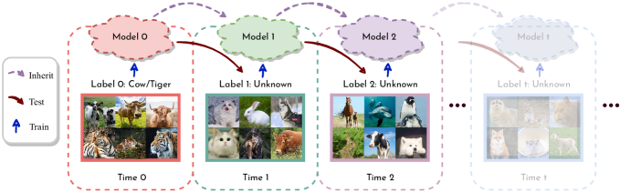
Figure 1: Illustration of the proposed EGZSL setting. At time 0, the model is trained with labeled seen class samples. In the subsequent time steps, the data is unlabeled, and its true class is uncertain (may be seen or unseen). Train: train the current model at each time step with only the data indicated by the arrows. Test: predict the current data with the model obtained in the last time step. Inherit: train the current model based on the model of the last time step.

1 Introduction

Deep neural networks (DNNs) have demonstrated powerful capabilities in various vision applications. However, existing algorithms are usually based on a large amount of once-given data, which makes it difficult to achieve the following two types of human-like intelligence: Deduction from the known to the unknown, and continually growing in practice with certain base knowledge.

In recognition tasks, the former intelligence requires the network to generalize to novel classes, known as Zero-Shot Learning (ZSL) [30, 15]. Traditional zero-shot research shares class information via pre-defined class semantics (e.g., human-annotated attributes [30] and word-vectors [41]), thereby enabling knowledge transfer between classes. The latter intelligence requires evolution during application (testing). The corresponding area is online learning [26], often used in scenarios with real-time requirements.

In this paper, we expect ZSL models to have unsupervised online boosting capability during the deployment phase. In the case of a ZSL model trained with seen classes only, it will suffer from the domain bias problem [18] and have difficulty recognizing unseen classes. However, existing ZSL research usually assumes a fixed model after training. Despite the availability of unseen class data during the deployment phase, it is difficult to use them to re-improve the model. Therefore, we propose a new setting named Evolutionary Generalized Zero-Shot Learning (EGZSL) to overcome this problem. Fig. 1 briefly depicts the training and testing process, where we allow the model to evolve continually from the unlabeled data stream. At time 0, a base model is trained with the same settings as in inductive GZSL (IGZSL) [6, 52]. At each subsequent time $t$, the model from time $t-1$ is first tested on the current batch of data, followed by unsupervised evolution. The model can only access the current data stream without having access to the base training data or other test data.

We compare the proposed setting to various limited-supervised and incremental learning tasks in Fig. 2. EGZSL has the following advantages compared to its counterparts:

(i) Mitigates the domain shift problem in IGZSL. It can improve the models gradually with the unlabeled test data during inference and lead to better recognition performance.

(ii) More suitable for real-world deployment. Compared to transductive GZSL [39, 46], there is no assumption of once-given data or of knowing whether test data is seen or unseen. In contrast to Continual GZSL [19, 43], there is no need for data labels in the evolutionary learning phase.

EGZSL meets three main challenges, as analyzed in Sec. 3.2. First is the typical catastrophic forgetting problem [35, 16] when training on streaming data. Secondly, due to the lack of unseen class samples in the base training, the prediction bias of the model is easily and consistently amplified when trained on the unlabeled data stream. Third, the model is vulnerable to potential data class imbalance problems. We then propose specific approaches to address these challenges. The overall framework is based on pseudo-label learning [32, 54], which is a common self-training approach for limited-supervised learning. We avoid forgetting by maintaining a global model, updated as the exponential moving average of the per-stage model. The historical information of the current model can be preserved by distilling it from the global model. We specify updateable class-related parameters for the class imbalance problem based on the data classes that occurred each time step. This avoids the error accumulation that causes predictions to deviate from certain classes. Moreover, we prevent confirmation bias by filtering noise labels. To avoid the effect of the initial prediction bias problem, we set a class-independent filtering threshold for each class. Finally, we propose evaluation criteria for this novel task, along with four baselines. The effectiveness of our proposed approach is demonstrated on three public ZSL benchmarks, on which the performance of our approach surpasses the base IGZSL method while other baselines fail. Our contributions are summarized as follows:

• We establish a more practical, albeit challenging, Evolutionary Generalized Zero-Shot Learning task that is more applicable to real-world deployments than existing ZSL settings.

• We analyze the main challenges of EGZSL and propose a targeted approach to address each of them.

• We determine the evaluation criteria for EGZSL and conduct extensive experiments on three public ZSL datasets. The proposed method consistently improves over baselines. The effectiveness of our method is demonstrated by a series of explanatory experiments.

2 Related work

Zero-Shot Learning (ZSL)

[30, 31, 52] aims at recognizing unseen classes when given only seen class samples. Early approaches [1, 13, 17]. typically embed images and semantic descriptors (e.g., attributes, word vectors) in the same space, then conducted a nearest neighbor search. However, these methods were sensitive to the domain shift problem [18]. They performed especially poorly in the Generalized Zero-Shot Learning (GZSL) setting [6, 52], which requires classifying both seen and unseen classes in the test phase. In the follow-up research, [51, 53, 42, 22, 8] employed conditional generative models [28, 2, 12] to generate pseudo-unseen class samples, thereby transferring GZSL into a common supervised task. [3, 36, 11] first distinguished seen or unseen classes with out-of-distribution detectors [14], then classified in the corresponding subset of classes. [55, 47] emphasized learning a deep embedding model by fine-tuning the backbone.

Transductive Zero-Shot Learning (TZSL)

[29, 39, 46, 38] assumes the unlabeled unseen test data is available during training. As a distinction, the earlier setting is called inductive ZSL. Most existing methods [18, 33, 56, 5] are based on pseudo-labeling strategies. [53, 38] also employed generative models. TZSL is a variant of semi-supervised learning [21] on ZSL, which is reasonable for research. It mitigates the domain shift problem and yields better recognition performance. However, for ZSL, the accessibility of unseen class samples in training is a too strong hypothesis, leading to limited application scenarios.

Continual Zero-Shot Learning (CZSL)

[7, 19, 43, 57] extended the traditional ZSL to a class-incremental paradigm, inspired by continual learning [40]. A-GEM [7] investigates the efficiency of lifelong learning methods and proposes a realistic evaluation protocol that learners should observe each example only once. It splits CUB and AWA into 20 and 10 disjoint subsets, respectively, and tests them on the ZSL setting, the first attempt at the lifelong setting for ZSL. Wei et al. [50] adjusted this setting and proposed lifelong zero-shot learning. They learned from all the seen classes of many datasets sequentially and evaluated all the unseen data with the learned model. Skorokhodov et al. [43] extended it to unlimited label searching space and let the model recognize unseen classes sequentially. Most later methods on CZSL are extended on top of this setting and focus on achieving better performance [20] or adapting to other applications. For example, Yi et al. [57] extended it to different domains, including painting and sketching, and introduced domain-aware continual zero-shot learning (DACZSL). In contrast, our EGZSL starts from the learned model with seen class samples, which were no longer available during the evolutionary process. We try to recognize the upcoming data, including both seen and unseen classes, and improve the model with them, aiming to boost the model’s recognition ability gradually.

Test Time Adaptation (TTA)

[44, 34, 48, 49] enables the model to better adapt the test domain by constructing self-supervised learning (SSL) tasks on test data. It is also extended into an online setting for continual improvement. Sun et al. [44] employed a rotation prediction task to update the model in test time, which also served as an auxiliary task in training. Liu et al. [34] evaluated the TTA performance under different distribution shifts and proposed to adopt contrastive learning as the SSL task. Wang et al. [48] eliminated the auxiliary task in the training phase and utilized the minimum entropy strategy as the optimization in the test phase. Existing TTA research has focused chiefly on the distribution shift task, i.e., domain adaptation [48, 49]. We propose extending the traditional ZSL setting with TTA, resulting in a more realistic setting than TGZSL and mitigating the domain shift problem in IGZSL. Due to the extreme class imbalance problem in the base training phase, the proposed EGZSL faces some specific problems in domain adaptation, as analyzed in Sec. 3.2.

3 EGZSL: Settings and Challenges

In this section, we formulate the EGZSL setting, analyze its key challenges, and compare it to other limited-supervision or incremental learning tasks. Fig. 2 illustrates the differences between EGZSL and other similar settings.

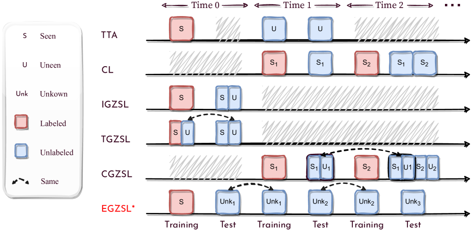
Figure 2: Comparasion of EGZSL with other similar settings. TTA: Test-Time Adaptation; CL: Continual Learning; IGZSL: Inductive Generalized Zero-Shot Learning; TGZSL: Transductive Generalized Zero-Shot Learning; CGZSL: Continual Generalized Zero-Shot Learning. In TTA, seen represents the source domain and unseen is the target domain. In other settings, the labeled classes that appear in the training set are denoted as seen, and vice versa are unseen. An unknown class means that it can be any class (in seen or unseen classes).

3.1 Problem Formulation

EGZSL aims to evolve continually from a data stream. Let $\mathcal{Y}^{s}$ and $\mathcal{Y}^{u}$ denote two disjoint class label sets ($\mathcal{Y}=\mathcal{Y}^{s}\cup\mathcal{Y}^{u}$). $\mathcal{X}\subseteq\mathbb{R}^{d_{\mathbf{x}}}$ and $\mathcal{A}\subseteq\mathbb{R}^{d_{\mathbf{a}}}$ are feature space and attribute space, respectively, where $d_{x}$ and $d_{a}$ are dimensions of these two spaces. In time 0, EGZSL learns an base model $f_{0}$ with a base set $\mathcal{D}^{b}=\{\mathbf{x}_{i},y_{i},{\mathbf{a}}_{y_{i}}|\mathbf{x}_{i}\in\mathcal{X},y_{i}\in\mathcal{Y}^{s},{\mathbf{a}}_{y_{i}}\in\mathcal{A}\}_{i=1}^{N_{b}}$, where $N_{b}$ is the base set data volume. The base model has a base ability to distinguish both seen and unseen classes, i.e., $f_{0}:\mathcal{X}\rightarrow\mathcal{Y}$. Then in time $1,...,t,...,T$, the base model is tested and evolved on the test data stream $\mathcal{D}^{te}_{1},...,\mathcal{D}^{te}_{t},...,\mathcal{D}^{te}_{T}$ and obtain $f_{1},...,f_{t},...,f_{T}$, where $\mathcal{D}^{te}_{t}=\{\mathbf{x}_{j},y_{j}|\mathbf{x}_{j}\in\mathcal{X},y_{j}\in\mathcal{Y}\}_{j=1}^{N_{t}}$. $N_{t}$ is the data amount in time $t$. Note that $\mathcal{D}^{te}_{t}$ is tested with $f_{t-1}$ and $f_{t-1}$ is retrained with the unlabeled data in $\mathcal{D}^{te}_{t}$. $f_{t}$ is hoped to have a better performance than $f_{t-1}$ in classifying data with label in $\mathcal{Y}$. We call the training on the labeled base set and on the unlabeled sequential test set base learning and evolutionary learning, respectively. Finally, EGZSL performance is evaluated with the test result on all the test subsets.

3.2 Challenges Analysis

Catastrophic problem. When training on the one-time given data, it is able to repeatedly utilize the data to reach the global optimum. On the contrary, there is a contradiction of falling into a local optimum and underutilization of data when training on the incremental data stream. Since only a small amount of data can be accessed at a time, overfitting on this batch of data will lead to catastrophic forgetting [35, 16] the previous knowledge. Conversely, the batch of data cannot be fully utilized, resulting in low training efficiency. Ensuring data utilization efficiency while preventing forgetting is a problem that needs to be solved.

Initial bias problem. Unlabeled training on the evolutionary data is influenced by the accuracy of the pseudo-labels predicted by the base model. However, when training the base model with unbalanced data classes, its prediction will be biased towards specific classes. This problem exists in EGZSL since the base set lacks unseen class samples. The prediction imbalance problem will cause error accumulation when continuing training with unbalanced pseudo-labels.

Sensitivity to data class bias. Since the EGZSL setting assumes arbitrary class distributions for the evolutionary learning phase, the model is at risk of being exposed to class-biased batch data. Training on biased data can lead to bias in the model predictions for pseudo-labeling the next phase, which in turn increases the model bias, ultimately causing a progressive impact on the sequential data.

3.3 EGZSL vs. Similar Settings

As shown in Fig. 2, we compare EGZSL to existing settings. In our setup, the aggregation of test data in all time periods is equivalent to the test data of the single test phase in inductive Generalized Zero-Shot Learning (IGZSL) and transductive Generalized Zero-Shot Learning (TGZSL). To put it in another perspective, EGZSL can be regarded as a strict version of TGZSL. TGZSL assumes that all labeled seen class data and unlabeled seen class and unseen class test data are given at once, along with a fixed test set and known seen-unseen class splitting in the test set. In contrast, the proposed EGZSL requires further improvements on arbitrary data without knowing its label or rough class splitting, which is more consistent with reality. Since there is no existing method for EGZSL, in the experiment, we consider IGZSL and TGZSL as upper and lower bounds for EGZSL to evaluate its performance.

4 Method

EGZSL extends the IGZSL setting in test time. Any existing IGZSL models can be employed in our setting without retraining on the base data. Since base learning has been well studied, we focus mainly on the evolutionary learning phase. This section describes our method and explains each component that promotes evolutionary learning.

At each time step $t$, we first predict the pseudo-label of current data (Sec. 4.1). To prevent catastrophic forgetting, we maintain a momentum model to preserve global data information (Sec. 4.2) and distill it to the current model. In addition, we select learnable class parameters (Sec. 4.3) to prevent class imbalance learning and filter unreliable data (Sec. 4.4) to avoid error accumulation. A specific training process is described in Algorithm 1.

4.1 Training with Pseudo Labels

Suppose a base model has been trained on the base set. We employ a pseudo-labeling strategy [32, 54] to enable continually improving from the unlabeled data, which is a typical technique in semi-supervised learning [32], and domain adaptation [48]. In time $t$, the pseudo label $\hat{y}_{\mathbf{x}}$ of a datum $\mathbf{x}$ is predicted with the highest compatibility with the model of the immediately preceding stage:

$$\begin{split}\hat{y}_{\mathbf{x}}=f_{t-1}(\mathbf{x})=\operatorname*{argmax}_{y}F_{t-1}(\mathbf{x},y,\mathbf{W}_{t-1}),\end{split}$$ (1)

where $F_{t-1}$ measures the compatibility score between $\mathbf{x}$ and any class $y$, and $\mathbf{W}_{t-1}$ denotes its parameter. Based on the pseudo labels, we use the cross-entropy for continued optimizing $\mathbf{W}_{t-1}$, i.e.,

$$\begin{split}\ell_{ce}(\mathbf{x})&=-\log p_{t-1}(\mathbf{x},\hat{y}_{\mathbf{x}},\mathcal{Y}),\\ p_{t-1}(\mathbf{x},y,\mathcal{Y})=&\frac{\exp(F_{t-1}(\mathbf{x},y,\mathbf{W}_{t-1}))}{\sum_{c\in\mathcal{Y}}\exp(F_{t-1}(\mathbf{x},c,\mathbf{W}_{t-1}))}.\end{split}$$ (2)

4.2 Maintenance of Global Information

A dilemma of EGZSL is the unavailability of all evolutionary data at the same time. Directly updating the model with gradient descent at a certain time step can lead to catastrophic forgetting [35, 16], which is a typical difficulty in sequential learning. We resort to the momentum updated model as the surrogate of historical information, similar to MoCo [23, 10]. Formally, the parameters of the momentum model are updated as exponential moving averages (EMA) on the previous time-step model parameters. Denoting $F_{ema}$ as the momentum model with parameters $\mathbf{W}_{ema}$, each time $t$, $\mathbf{W}_{ema}$ is updated as

$$\begin{split}\mathbf{W}_{ema}=m_{1}\cdot\mathbf{W}_{ema}+(1-m_{1})\cdot\mathbf{W}_{t},\end{split}$$ (3)

where $m_{1}\in[0,1)$ is a smoothing factor. We update $\mathbf{W}_{ema}$ with the gradient detached. $\mathbf{W}_{ema}$ is considered to maintain the global information at historical time steps, which changes more smoothly than $\mathbf{W}_{t}$. We distill [25] this information to the current model with Kullback-Leibler (KL) divergence:

$$\begin{split}\ell_{kl}(\mathbf{x})=\sum_{y\in\mathcal{Y}}p_{t}(\mathbf{x},y,\mathcal{Y})\log\frac{p_{t}(\mathbf{x},y,\mathcal{Y})}{p_{ema}(\mathbf{x},y,\mathcal{Y})}.\end{split}$$ (4)

Here $p_{t}(\mathbf{x},y,\mathcal{Y})$ and $p_{ema}(\mathbf{x},y,\mathcal{Y})$ denote the probability distribution over the variable $y$. Note that at each time step $t$, $\mathbf{W}_{ema}$ is updated after $\mathbf{W}_{t}$. With the distillation loss, the model can learn from the current data stream while avoiding catastrophic forgetting of previous information. This creates conditions for balancing the data utilization efficiency (Sec. 3.2).

4.3 Class Selection for Stable Training

As stated in Sec. 3.2, the potential imbalance of data classes in the evolutionary stage tends to make the trained model predictions unbalanced and cause error accumulation. This problem is particularly severe when the number of samples available at each time step is small. It is prone to missing samples in certain classes, and cross-entropy based on pseudo-hard labels may produce sharper constraints that cause model predictions to abruptly deviate from these classes. We mitigate this problem by selecting specific class parameters to be updated for each time step. Consider typical GZSL classifiers are implemented with a linear model, i.e., $\mathbf{W}$ is a matrix with rows $|\mathcal{Y}|$ and columns $d_{\mathbf{x}}$:

$$\begin{split}F(\mathbf{x},y,\mathbf{W}):=\mathbf{W}_{y}\cdot\mathbf{x}.\end{split}$$ (5)

In order to make the corresponding weights of each class change more smoothly, in time step $t$, we select all the classes that appear in the pseudo labels, i.e.,

$$\begin{split}\mathcal{Y}_{t}^{sel}=\mathrm{unique}(\{\hat{y}_{\mathbf{x}}\}_{\mathbf{x}\in\mathcal{D}_{t}^{te}}).\end{split}$$ (6)

Here $\mathrm{unique}(\cdot)$ denotes returning the unique elements of the label set, which can be achieved by calling the pytorch function directly. Finally, the cross-entropy loss in Eq. (2) is replaced with

$$\begin{split}\ell_{ce}^{sel}(\mathbf{x})&=-\log p_{t-1}(\mathbf{x},\hat{y}_{\mathbf{x}},\mathcal{Y}_{t}^{sel}).\end{split}$$ (7)

Note that $\ell_{kl}$ in Eq. (4) is still calculated with the full label set $\mathcal{Y}$.

4.4 Data Selection for Effective Training

Since the unlabeled data is trained with the pseudo-labeling strategy, noisy pseudo-labels will cause e confirmation bias. Therefore, in each time step, we use the model obtained in the previous stage to select samples with low uncertainty. The uncertainty reflects the confidence level of the model prediction, typically measured by entropy or max softmax prediction [37]. We use the latter to select samples with more reliable pseudo labels. Intuitively, we can set a constant threshold to filter the samples whose softmax prediction does not exceed this value, i.e.,

$$\begin{split}\texttt{M}(\mathbf{x})=\mathds{1}(\max_{y}p_{t-1}(\mathbf{x},y,\mathcal{Y})>\tau),\end{split}$$ (8)

where $\mathds{1}$ is the indicator function, and $\tau\in(0,1]$ is the pre-defined threshold. $\texttt{M}(\cdot)$ enables the selection of the samples with high confidence. However, in the case where the value of softmax prediction is unbalanced across classes, using a fixed threshold leads to unbalanced class selection. For example, the base model is trained only on the seen classes, resulting in a model with larger confidence in the seen class samples and lower confidence in the unseen class samples. Using the fixed threshold strategy leads to filtering too many unseen class samples. Selection imbalance in sequential data learning will cause Matthew Effect.

We thereby employ an adaptive threshold for each class. Considering the reason for the imbalance selection is the class variation of softmax prediction distributions, we can use its class statistics to develop class-independent thresholds. Specifically, we adopt a curriculum learning strategy [4] to take into account the learning status of each class. Since only a small number of samples are available in one time step, we count all historical time steps to calculate the class confidence statistics. The statistics are momentum updated as

$$\begin{split}\delta_{ema}(y)&=m_{2}\cdot\delta_{ema}(y)+(1-m_{2})\cdot\delta_{t-1}(y),\\ \delta_{t-1}(y&)=\frac{1}{N_{t}^{y}}\sum_{\mathbf{x}\in\mathcal{D}^{te}_{t}}\mathds{1}(y=\hat{y}_{\mathbf{x}})p_{t-1}(\mathbf{x},\hat{y}_{\mathbf{x}},\mathcal{Y}),\end{split}$$ (9)

where $m_{2}\in[0,1)$ is a momentum coefficient, and $N_{t}^{y}=\sum_{\mathbf{x}\in\mathcal{D}^{te}_{t}}\mathds{1}(y=\hat{y}_{\mathbf{x}})$ ($\hat{y}_{\mathbf{x}}$ is defined in Eq. (1)). $\delta_{t-1}(y)$ represents the averaged softmax prediction regarding class $y$, predicted by the immediately preceding stage model. $\delta_{ema}$ serves as the surrogate of the class learning status which is updated before data selection in time $t$. It can then be used to scale the fixed threshold $\tau$. The scaled data mask is

$$\begin{split}\texttt{M}_{scl}(\mathbf{x})=\mathds{1}((\mathbf{x},f_{t-1}(\mathbf{x}))>\delta_{t-1}(f_{t-1}(\mathbf{x}))\cdot\tau).\end{split}$$ (10)

$\texttt{M}_{scl}(\cdot)$ is then used as a weighting factor for the loss of each datum to achieve data selection, i.e.,

Notably, the class and data selection processes only incur negligible extra computation.

Algorithm 1 The Proposed EGZSL Method

Input: Data $\{\mathbf{x}_{i}\}_{i=1}^{N_{t}}$ in dataset $\mathcal{D}_{t}^{te}$; Model $f_{t-1}$ with parameters $\mathbf{W}_{t-1}$; Momentum model $f_{ema}$ with parameters $\mathbf{W}_{ema}$; Class momentum confidence $\delta_{ema}$; Hyper-parameters $m_{1},m_{2},\tau,\lambda$.

1:Predict pseudo-label: $\hat{y}_{\mathbf{x}}=f_{t-1}(\mathbf{x})$.

2:Select training classes by Eq. 6.

3:Update class momentum confidence by Eq. 9.

4:Calculate data mask by Eq. 10.

5:Update $\mathbf{W}_{t-1}$ by cross-entropy loss and KL divergence loss in Eq. 12.

6:Update momentum model by Eq. 3.

Output: Prediction $\{f_{t-1}(\mathbf{x})|\mathbf{x}\in\mathcal{D}_{t}^{te}\}$; Updated model $f_{t}$; Updated momentum model $f_{ema}$; Updated class momentum confidence $\delta_{ema}$.

4.5 Overall Objectives

Overall, the total objective loss function each time $t$ is

$$\mathcal{L}_{all}=\mathcal{L}_{ce}^{sel}+\lambda\mathcal{L}_{kl},$$ (12)

where $\lambda$ is a hyper-parameter for balancing loss $\mathcal{L}_{ce}^{sel}$ and $\mathcal{L}_{kl}$. Algorithm 1 describes the concrete training process in one evolutionary learning step.

5 Experiments

In this section, we propose a protocol for evaluating EGZSL methods and compare the performance of our method to potential upper and lower boundaries. We also report on further experiments that shed light on the working mechanisms of our method by isolating the effects of individual components.

5.1 Benchmark Protocol

Evaluation Procedure.

Since there is no existing benchmark protocol for evaluating EGZSL performance, we propose the following evaluation procedure: for a given ZSL dataset, the original training set is regarded as the base set, and the test set is divided into different batches in a fixed random order. Each method is first trained on the base set, then the prediction and updates are performed online on the divided test data stream. Note that the results of the current time step are predicted with the model of the last step. We introduce two instantiations of the above test data splitting for each following dataset: we use all test data in batches of 10 or 100 samples at a time. The rest data is only for testing. 1 gives an example of evolving with 100 samples once. To facilitate comparison with traditional GZSL methods, we employ the same metrics [52] as GZSL. EGZSL performance is evaluated based on the aggregation of the results across all test datasets. The measurement is the harmonic mean ($\mathit{H}$) of the average per-class top-1 accuracies in the seen ($\mathit{A}^{s}$) and unseen ($\mathit{A}^{u}$) classes. We run each benchmark five times with different random data orders and reports averages and standard deviations of the results.

Datasets.

We evaluate EGZSL methods on three public ZSL benchmarks: 1) Animals with Attributes 2 (AWA2) [31] contains 50 animal species and 85 attribute annotations, accounting for 37,322 samples. 2) Attribute Pascal and Yahoo (APY) [15] includes 32 classes of 15,339 samples and 64 attributes. 3) Caltech-UCSD Birds-200-2011 (CUB) [45] consists of 11,788 samples of 200 bird species, annotated by 312 attributes. We split the data into seen and unseen classes according to the common GZSL benchmark procedure in [52]. We follow [52] to adapt the 2048-dimensional visual representation (instead of the original images) extracted from the pre-trained ResNet101 [24].

	AWA2	APY	CUB
Test	13795	9407	4731
Task	137	94	47
Rest	95	7	31

Table 1: AWA2, APY, and CUB datasets, in terms of the number of total test data, evolutionary tasks, and rest samples in the case of owning 100 samples in one evolutionary task.

5.2 Implementation Details

Model.

Since the base learning phase setting is the same as the IGZSL, we directly borrow the off-the-shelf IGZSL model for EGZSL experiments. We construct our EGZSL method on the linear classifiers (Eq. 5) trained by ZLA [8]. We report the results of our own implementation since the official trained models are not available. Please refer to its original paper for the base phase training procedure.

Optimization.

We employ the Adam optimizer [27] with a learning rate of $5e$-$5$ for the main experiments. We set the (mini) batch size equal to the total number of data in each evolutionary stage. Each stage of data is optimized for one epoch only.

	Method	AWA2			CUB			APY
		$\mathit{A}^{u}$	$\mathit{A}^{s}$	$\mathit{H}$	$\mathit{A}^{u}$	$\mathit{A}^{s}$	$\mathit{H}$	$\mathit{A}^{u}$	$\mathit{A}^{s}$	$\mathit{H}$
$\mathcal{T}$	COND [33]	80.2	90.0	84.8	57.0	68.7	62.3	51.8	87.6	65.1
	TF-VAEGAN [38]	87.3	89.6	88.4	69.9	72.1	71.0	-	-	-
	STHS [5]	94.9	92.3	93.6	77.4	74.5	75.9	-	-	-
$\mathcal{I}$	COND [33]	56.4	81.4	66.7	47.4	47.6	47.5	26.5	74.0	39.0
	FREE [9]	60.4	75.4	67.1	55.7	59.9	57.7	-	-	-
	Chou et al. [11]	65.1	78.9	71.3	41.4	49.7	45.2	35.1	65.5	45.7
	GCM-CF [58]	60.4	75.1	67.0	61.0	59.7	60.3	37.1	56.8	44.9
	ZLA [8]	65.4	82.2	72.8	50.9	58.4	54.4	38.4	60.3	46.9
$\mathcal{E}$	ZLA+ERM@10	$54.2\pm 6.5$	$60.4\pm 3.1$	$56.9\pm 4.2$	$45.2\pm 4.3$	$42.7\pm 4.0$	$43.9\pm 4.0$	$8.6\pm 0.2$	$0.4\pm 0.3$	$0.9\pm 0.4$
	ZLA+ERM@100	$55.0\pm 3.1$	$64.6\pm 2.5$	$59.4\pm 2.7$	$\bf 52.0\pm 0.7$	$51.2\pm 0.7$	$51.6\pm 0.6$	$11.5\pm 1.4$	$5.1\pm 0.9$	$6.8\pm 0.5$
	ZLA+ours@10	$65.4\pm 0.6$	$\bf 85.8\pm 0.5$	$74.2\pm 0.2$	$51.0\pm 0.3$	$\bf 58.9\pm 0.3$	$\bf 54.6\pm 0.1$	$39.1\pm 1.1$	$\bf 60.1\pm 1.1$	$47.3\pm 0.8$
	ZLA+ours@100	$\bf 73.3\pm 1.0$	$81.3\pm 0.8$	$\bf 77.0\pm 0.2$	$51.7\pm 0.6$	$57.9\pm 0.3$	$54.6\pm 0.3$	$\bf 40.0\pm 1.0$	$58.6\pm 0.7$	$\bf 47.5\pm 0.8$

Table 2: Performance comparison between the proposed baselines and with sota IGZSL and TGZSL methods. $\mathcal{T}$, $\mathcal{I}$, and $\mathcal{E}$ denote the methods under TGZSL, IGZSL, and EGZSL settings, respectively. @10 and @100 correspond to the amount of data accessed in a single evolutionary time step. $\mathit{A}^{u}$ and $\mathit{A}^{s}$ represent per-class accuracy scores (%) on seen and unseen test sets, and $\mathit{H}$ is their harmonic mean. The best result is bolded.

5.3 Main Results

Baselines.

We propose four baselines for EGZSL setting based on ZLA [8]. Two baselines assemble with our proposed method. The other two simply use pseudo-label-based empirical risk minimization (ERM), for comparison with our method. We also compare the results with IGZSL and TGZSL methods, which construct the potential lower and upper bound of EGZSL performance.

Results.

Tab. 2 presents our main experimental results, according to which we have the following findings:

Our method brings gains to the IGZSL baseline, whereas simple ERM fails. In unsupervised data stream learning, the row method without considering catastrophic forgetting, prediction bias, and data bias (Sec. 3.2) is unable to provide reliable gradients. It yields crashed results when the initial model is largely biased (APY). In contrast, the superior results of our method verify its ability to deal with the above problems.

Coarse-grained datasets (i.e., AWA2, APY) enjoy more evolutionary gains compared to the fine-grained dataset (i.e., CUB). This is because the evolutionary learning process mainly compensates for the visual bias [18] caused by missing unseen classes during base training. This problem is more severe in coarse-grained datasets and therefore results in more performance gains when mitigated. The small amount of evolutionary data per class on average (23 in CUB vs. 275 in AWA2) is also an external cause of modest improvement in CUB.

The performance improvement is slightly larger when more data is provided each time step. Accessing more data at once can reduce the risk of being dominated by noisy pseudo-label samples and provide a more stable gradient. In a real-world deployment, the number of single evolution samples can be selected according to actual needs and resource usage.

Although our method surpasses the IGZSL baseline, there is still a large gap between its performance and that of the methods in the TGZSL setting. This is primarily because (i) TGZSL provides all the test data at once, allowing repeatably training on it until convergence; (ii) TGZSL provides prior information about whether the test data belong to the seen or unseen class, which is a much more relaxed setting; (iii) TGZSL has been well studied, while EGZSL still has more room for development. Nevertheless, the EGZSL setting is better suited for real-world deployments and has greater application potential.

5.4 Evolution Curves

To compare the performance of models at different time steps, we plot its variation curve as the evolutionary task proceeds. Since the test data varies in different tasks, we obtain the evolution curve with all test data. This is within the TGZSL setting and is legitimate as an explanatory experiment. We conduct this experiment on AWA2 and APY. As shown in Fig. 3, overall performance tends to increase over time. The accuracy rises faster in the early stages and then gradually converges. This is because the main contradiction of ZSL i.e., the domain shift problem [18], is quickly alleviated in the early stage after supplementing the visual information of the unseen class. After the conflicts caused by this problem are reduced, the performance improvement gradually slows down in the later stages.

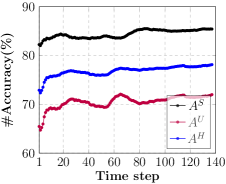
(a)

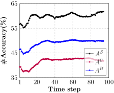
(b)

Figure 3: (a), (b) Evolution curves with 100 data per task. Accuracy increases as the task progress.

	Baseline	AWA2			APY
		$\mathit{A}^{u}$	$\mathit{A}^{s}$	$\mathit{H}$	$\mathit{A}^{u}$	$\mathit{A}^{s}$	$\mathit{H}$
(i)	W/O Momentum Model	57.2	80.2	66.7	17.8	45.5	25.6
(ii)	W/O Class Selection	66.4	72.9	69.5	39.1	51.3	44.4
(iii)	W/O Data Selection	62.3	86.7	72.5	38.7	57.3	46.2
(iv)	Adaptive$\rightarrow$fixed thre.	57.4	86.2	68.9	27.6	50.4	35.7
	Full model	$65.9$	85.5	74.4	38.6	61.5	47.4

Table 3: Ablation study results of the proposed method on AWA2 and APY datasets (with data amount of 10 per evolutionary task).

5.5 Ablation Analysis

We validated the effectiveness of our motivation and design via the following baselines, with the results shown in Tab. 3. The results are obtained with a fixed random seed. (i) W/O Momentum Model. We first explore the effect of momentum model (Sec. 4.2), which helps preserve the historical information. As shown in Tab. 3, the ablation of this component degrades the performance on both two datasets. The performance degradation is especially serious in the case of low initial accuracy (APY). In the absence of historical information, noisy pseudo-labels dominate the training process. This demonstrates the importance of suppressing catastrophic forgetting in training with streaming data.

(ii) W/O Class Selection. We also evaluate the importance of the class selection module (Sec. 4.3). As is previously discussed, this module prevents the adverse effects of potentially imbalanced data classes, thus the results are not promising when ablating it.

(iii) W/O Data Selection. This baseline removes the operations defined by Eq. (9), (10), and (11). The removal of data selection implies that all samples are involved in the training. The drop in performance accords with our intuition to filter the low-confidence samples.

(iv) Adaptive$\rightarrow$fixed thre. To demonstrate the effectiveness of the adaptive threshold strategy in data selection, we also test it with a fixed threshold. This baseline is also described in Sec. 4.4 that replaces Eq. (10) with Eq. (9). We set $\tau$ to 0.8 for the best results of this baseline, but the performance is even worse than without data selection. This validates our analysis (Sec. 4.4) that a fixed threshold comes with the risk of data class imbalance.

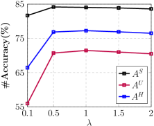
(a)

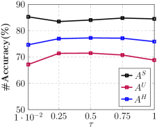
(b)

(c)

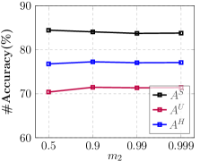
(d)

Figure 4: Hyperparameters w.r.t. EGZSL performance on AWA2. (a) Effects of loss balancing coefficient $\lambda$ (Eq. 12). (b) Effects of different thresholds $\tau$ in Eq. (10). (c), (d) Effects of the smoothing factors $m_{1}$ and $m_{2}$ in Eq. (3) and (9).

5.6 Hyperparameters

We study the influence of the loss weighting coefficient $\lambda$, the threshold $\tau$, and the momentum coefficients $m_{1}$ and $m_{2}$, which are reported in Fig. 4. Though the performance under different settings of hyperparameters varies, our method is overall stable. The results are more sensitive to $\lambda$ and $m_{1}$ since these two parameters are related to catastrophic forgetting. In contrast, $\tau$ and $m_{2}$, two variables related to data selection, have a slightly smaller fluctuation in performance. We set $\lambda$ to 1, $\tau$ to 0.5, $m_{1}$ to 0.99, and $m_{2}$ to 0.9 for best results. More experiments can be found in the supplementary material.

6 Conclusion

In this paper, we propose a novel and more realistic GZSL setting — Evolutionary GZSL. It starts from the traditional learned GZSL models without the seen data, and gradually boosts itself by simultaneously recognizing and learning from the unlabeled test data. To evaluate the proposed EGZSL, we design a new protocol by randomly dividing the datasets into episodic training and testing with multi time steps. In addition, we also propose a method to solve this task and give the baseline results on three benchmark datasets, and the results show its feasibility and superiority compared with several traditional methods.

Acknowledgments

This work was partly supported by the National Natural Science Foundation of China (NSFC) under Grant Nos. 61872187, 62077023, and 62072246, partly by the Natural Science Foundation of Jiangsu Province under Grant No. BK20201306, and partly by the “111 Program” under Grant No. B13022.

	Method	AWA2			CUB			APY
		$\mathit{A}^{u}$	$\mathit{A}^{s}$	$\mathit{H}$	$\mathit{A}^{u}$	$\mathit{A}^{s}$	$\mathit{H}$	$\mathit{A}^{u}$	$\mathit{A}^{s}$	$\mathit{H}$
$\mathcal{T}$	COND [26]	80.2	90.0	84.8	57.0	68.7	62.3	51.8	87.6	65.1
$\mathcal{I}$	COND [26]	51.6	80.5	62.9	44.9	54.5	49.2	31.2	59.4	40.9
$\mathcal{E}$	COND+ERM@10	$51.9\pm 0.3$	$75.5\pm 0.2$	$61.5\pm 0.3$	$41.1\pm 0.4$	$45.4\pm 0.5$	$43.1\pm 0.3$	$26.3\pm 0.4$	$45.8\pm 0.8$	$33.4\pm 0.5$
	COND+ERM@100	$51.2\pm 0.3$	$74.7\pm 0.4$	$60.1\pm 0.1$	$36.3\pm 0.3$	$39.6\pm 0.7$	$37.9\pm 0.4$	$25.4\pm 1.1$	$43.0\pm 0.6$	$32.0\pm 0.8$
	COND+ours@10	$57.1\pm 0.5$	$\bf 82.1\pm 0.1$	$67.4\pm 0.3$	$\bf 45.2\pm 0.1$	$54.6\pm 0.1$	$49.4\pm 0.1$	$32.1\pm 0.7$	$\bf 60.1\pm 0.2$	$41.9\pm 0.6$
	COND+ours@100	$\bf 59.2\pm 1.1$	$80.7\pm 0.4$	$\bf 68.3\pm 0.8$	$45.0\pm 0.2$	$\bf 55.2\pm 0.3$	$\bf 49.6\pm 0.1$	$\bf 35.2\pm 0.2$	$58.0\pm 0.6$	$\bf 43.8\pm 0.2$

Table A.4: Evolution results on COND. $\mathcal{T}$, $\mathcal{I}$, and $\mathcal{E}$ denote the methods under TGZSL, IGZSL, and EGZSL settings, respectively. @10 and @100 correspond to the amount of data accessed in a single evolutionary time step. $\mathit{A}^{u}$ and $\mathit{A}^{s}$ represent per-class accuracy scores (%) on seen and unseen test sets, and $\mathit{H}$ is their harmonic mean. The best result is bolded.

Appendix

Appendix A Experimental Details

A.1 Main Experiments

The ERM method in Sec. 5.3 used for the comparison is optimized by a pseudo-label-based cross-entropy loss on the entire data at each time step without any additional means. Since the data batch size is related to the learning rate selection, we use a lower learning rate of $5e$-$6$ for a single-step evolution data size of 10 and $5e$-$5$ for 100.

A.2 Hyperparameters

The hyperparameter analysis in Sec. 5.6 is conducted with a data amount of 100 per evolutionary task. We have also provided the analysis on the CUB and APY datasets in Sec. B.4.

Appendix B Additional Experiments

B.1 EGZSL Training Based on COND

In Sec. 5.3 we have done our EGZSL experiments with ZLA [6]. In this section, we test the evolution performance on COND [26] to show the generality of the proposed method. We re-implement the COND method ourselves for comparison with its IGZSL performance. We set $\tau=1$, $m_{1}=0.99$, and $m_{2}=0.9$ on the three datasets for the best results. $\lambda$ is set to 1, 5, and 1.5 on AWA2, CUB, and APY, respectively. The results are present in Tab. A.4. The performance gain is similar to that on ZLA, demonstrating our method’s generality. One slight difference from the one on ZLA is that ERM’s results on APY do not crash. This may be due to differences in the base method, for which we do not provide in-depth analysis here since it is orthogonal to our main claim.

B.2 Evolution Curves on CUB

In Sec. 5.4 we have shown the evolution curves for AWA2 and APY. Here we provide the evolution curve for CUB, as depicted in Fig. A.5. Overall performance volatility goes up. According to this trend, more evolutionary tasks are needed for the fine-grained dataset CUB to achieve performance convergence.

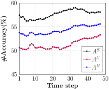
Figure A.5: (a), (b) Evolution curves on CUB. Accuracy increases as the task progress.

	Baseline	AWA2			CUB			APY
		$\mathit{A}^{u}$	$\mathit{A}^{s}$	$\mathit{H}$	$\mathit{A}^{u}$	$\mathit{A}^{s}$	$\mathit{H}$	$\mathit{A}^{u}$	$\mathit{A}^{s}$	$\mathit{H}$
(i)	W/O Momentum Model	57.2	80.2	66.7	48.6	59.1	53.3	17.8	45.5	25.6
(ii)	W/O Class Selection	66.4	72.9	69.5	53.2	50.1	51.6	39.1	51.3	44.4
(iii)	W/O Data Selection	62.3	86.7	72.5	50.7	59.1	54.6	38.7	57.3	46.2
(iv)	Adaptive$\rightarrow$fixed thre.	57.4	86.2	68.9	51.0	58.3	54.4	27.6	50.4	35.7
	Full model	$65.9$	85.5	74.4	$50.8$	59.2	54.7	38.6	61.5	47.4

Table A.5: Ablation study results with data amount of 10 per evolutionary task.

	Baseline	AWA2			CUB			APY
		$\mathit{A}^{u}$	$\mathit{A}^{s}$	$\mathit{H}$	$\mathit{A}^{u}$	$\mathit{A}^{s}$	$\mathit{H}$	$\mathit{A}^{u}$	$\mathit{A}^{s}$	$\mathit{H}$
(i)	W/O Momentum Model	52.3	77.1	62.3	42.2	50.1	45.8	28.2	27.6	27.9
(ii)	W/O Class Selection	74.4	79.3	76.8	51.8	43.9	47.5	42.5	52.0	46.8
(iii)	W/O Data Selection	71.5	83.4	77.0	51.2	57.1	54.0	40.4	56.7	47.2
(iv)	Adaptive$\rightarrow$fixed thre.	62.8	82.8	71.5	50.7	56.7	53.5	36.8	56.9	44.7
	Full model	$71.5$	84.1	77.3	51.5	58.1	54.6	41.3	60.7	49.2

Table A.6: Ablation study results with data amount of 100 per evolutionary task.

B.3 Additional Ablation Study

We provide the ablation results on all datasets and the results when the data amount per evolutionary task is 100 as a supplement to Sec. 5.5. The results are obtained with a fixed random seed. We use a lower learning rate of $5e$-$6$ for a single-step evolution data size of 10 and $5e$-$5$ for 100 as in Sec. A.1.

As shown in Tab. A.5 and A.6, ablating each module can lead to performance degradation, and the overall trend is roughly the same as the partial results provided in Sec. 5.5. The accuracy of the unseen class becomes greater when the class selection strategy is not employed, which we conjecture is due to the over-calibration strategy employed by ZLA. It causes more samples to be predicted as unseen classes, resulting in class biased learning during the evolutionary process.

An additional phenomenon is that the performance gains of class selection and data selection strategies on AWA2 are smaller when 100 data points are available for each task than when only 10 data points are available. This is because when enough data are used in one update (100 is greater than the number of classes in the AWA2 dataset), the class bias problem itself is minimal. In addition, with sufficient base model performance, the large batch data ensures that learning avoids being dominated by noisy pseudo-labeled samples. In deployment, the timing of online model updates can be chosen based on actual resource usage.

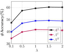
(a)

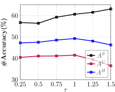
(b)

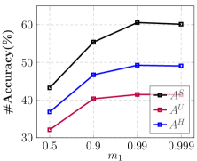
(c)

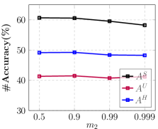
(d)

Figure A.6: Hyperparameters w.r.t. EGZSL performance on APY dataset. (a) Effects of loss balancing coefficient $\lambda$ (Eq. (12)). (b) Effects of different thresholds $\tau$ in Eq. (10). (c), (d) Effects of the smoothing factors $m_{1}$ and $m_{2}$ in Eq. (3) and (9).

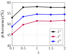
(a)

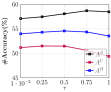
(b)

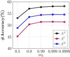
(c)

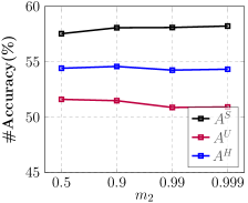
(d)

Figure A.7: Hyperparameters w.r.t. EGZSL performance on CUB dataset. (a) Effects of loss balancing coefficient $\lambda$ (Eq. (12)). (b) Effects of different thresholds $\tau$ in Eq. (10). (c), (d) Effects of the smoothing factors $m_{1}$ and $m_{2}$ in Eq. (3) and (9).

B.4 Hyperparameter Analysis on APY and CUB

In Sec. 5.6 we have shown the hyperparameter analysis results on AWA2. For completeness, in Fig. A.6 and A.7 we provide the EGZSL performance w.r.t. hyperparameters on the APY and CUB datasets. This experiment is conducted with a data amount of 100 per evolutionary task. Larger (than on AWA2) $\lambda$ and $\tau$ values promotes better EGZSL performance on APY. This is due to the poor performance of the base model on APY, which requires more strict data filtering and historical information maintenance for stable evolution. We obtain the best EGZSL performance on CUB when $m_{1}=0.999$; other parameters are the same as those on AWA2. We set $\lambda=1.5$, $\tau=1$, $m_{1}=0.99$, and $m_{2}=0.9$ for APY.

References

- [1] Zeynep Akata, Florent Perronnin, Zaid Harchaoui, and Cordelia Schmid. Label-embedding for attribute-based classification. In CVPR, pages 819–826, 2013.
- [2] Martin Arjovsky, Soumith Chintala, and Léon Bottou. Wasserstein generative adversarial networks. In ICML, pages 214–223, 2017.
- [3] Yuval Atzmon and Gal Chechik. Adaptive confidence smoothing for generalized zero-shot learning. In CVPR, pages 11671–11680, 2019.
- [4] Yoshua Bengio, Jérôme Louradour, Ronan Collobert, and Jason Weston. Curriculum learning. In ICML, pages 41–48, 2009.
- [5] Liu Bo, Qiulei Dong, and Zhanyi Hu. Hardness sampling for self-training based transductive zero-shot learning. In CVPR, pages 16499–16508, 2021.
- [6] Wei-Lun Chao, Soravit Changpinyo, Boqing Gong, and Fei Sha. An empirical study and analysis of generalized zero-shot learning for object recognition in the wild. In ECCV, pages 52–68, 2016.
- [7] Arslan Chaudhry, Marc’Aurelio Ranzato, Marcus Rohrbach, and Mohamed Elhoseiny. Efficient lifelong learning with a-gem. In ICLR, 2019.
- [8] Dubing Chen, Yuming Shen, Haofeng Zhang, and Philip H.S. Torr. Zero-shot logit adjustment. In IJCAI, pages 813–819, 2022.
- [9] Shiming Chen, Wenjie Wang, Beihao Xia, Qinmu Peng, Xinge You, Feng Zheng, and Ling Shao. Free: Feature refinement for generalized zero-shot learning. In ICCV, 2021.
- [10] Xinlei Chen, Haoqi Fan, Ross Girshick, and Kaiming He. Improved baselines with momentum contrastive learning. arXiv preprint arXiv:2003.04297, 2020.
- [11] Yu-Ying Chou, Hsuan-Tien Lin, and Tyng-Luh Liu. Adaptive and generative zero-shot learning. In ICLR, 2021.
- [12] Laurent Dinh, David Krueger, and Yoshua Bengio. Nice: Non-linear independent components estimation, 2014.
- [13] Mohamed Elhoseiny, Babak Saleh, and Ahmed Elgammal. Write a classifier: Zero-shot learning using purely textual descriptions. In ICCV, pages 2584–2591, 2013.
- [14] Zhen Fang, Yixuan Li, Jie Lu, Jiahua Dong, Bo Han, and Feng Liu. Is out-of-distribution detection learnable? In NeurIPS, 2022.
- [15] Ali Farhadi, Ian Endres, Derek Hoiem, and David Forsyth. Describing objects by their attributes. In CVPR, pages 1778–1785, 2009.
- [16] Robert M French. Catastrophic forgetting in connectionist networks. Trends in cognitive sciences, 3(4):128–135, 1999.
- [17] Andrea Frome, Greg Corrado, Jonathon Shlens, Samy Bengio, Jeffrey Dean, Marc’Aurelio Ranzato, and Tomas Mikolov. Devise: A deep visual-semantic embedding model. In NeurIPS, page 2121–2129, 2013.
- [18] Yanwei Fu, Timothy M Hospedales, Tao Xiang, Zhenyong Fu, and Shaogang Gong. Transductive multi-view embedding for zero-shot recognition and annotation. In ECCV, pages 584–599. Springer, 2014.
- [19] Chandan Gautam, Sethupathy Parameswaran, Ashish Mishra, and Suresh Sundaram. Generalized continual zero-shot learning. arXiv preprint arXiv:2011.08508, 2020.
- [20] Subhankar Ghosh. Dynamic vaes with generative replay for continual zero-shot learning. arXiv preprint arXiv:2104.12468, 2021.
- [21] Yves Grandvalet and Yoshua Bengio. Semi-supervised learning by entropy minimization. In NeurIPS, volume 17, 2004.
- [22] Zongyan Han, Zhenyong Fu, Shuo Chen, and Jian Yang. Contrastive embedding for generalized zero-shot learning. In CVPR, pages 2371–2381, 2021.
- [23] Kaiming He, Haoqi Fan, Yuxin Wu, Saining Xie, and Ross Girshick. Momentum contrast for unsupervised visual representation learning. In CVPR, pages 9729–9738, 2020.
- [24] Kaiming He, Xiangyu Zhang, Shaoqing Ren, and Jian Sun. Deep residual learning for image recognition. In CVPR, pages 770–778, 2016.
- [25] Geoffrey Hinton, Oriol Vinyals, and Jeff Dean. Distilling the knowledge in a neural network. In NeurIPS, 2015.
- [26] Steven CH Hoi, Doyen Sahoo, Jing Lu, and Peilin Zhao. Online learning: A comprehensive survey. Neurocomputing, 459:249–289, 2021.
- [27] Diederik P Kingma and Jimmy Ba. Adam: A method for stochastic optimization. In ICLR, 2015.
- [28] Diederik P Kingma and Max Welling. Auto-encoding variational bayes. In ICLR, 2013.
- [29] Elyor Kodirov, Tao Xiang, Zhenyong Fu, and Shaogang Gong. Unsupervised domain adaptation for zero-shot learning. In ICCV, pages 2452–2460, 2015.
- [30] Christoph H Lampert, Hannes Nickisch, and Stefan Harmeling. Learning to detect unseen object classes by between-class attribute transfer. In CVPR, pages 951–958, 2009.
- [31] Christoph H Lampert, Hannes Nickisch, and Stefan Harmeling. Attribute-based classification for zero-shot visual object categorization. IEEE TPAMI, pages 453–465, 2013.
- [32] Dong-Hyun Lee et al. Pseudo-label: The simple and efficient semi-supervised learning method for deep neural networks. In ICML work shop, page 896, 2013.
- [33] Kai Li, Martin Renqiang Min, and Yun Fu. Rethinking zero-shot learning: A conditional visual classification perspective. In ICCV, pages 3583–3592, 2019.
- [34] Yuejiang Liu, Parth Kothari, Bastien van Delft, Baptiste Bellot-Gurlet, Taylor Mordan, and Alexandre Alahi. Ttt++: When does self-supervised test-time training fail or thrive? In NeurIPS, volume 34, pages 21808–21820, 2021.
- [35] Michael McCloskey and Neal J Cohen. Catastrophic interference in connectionist networks: The sequential learning problem. In Psychology of learning and motivation, volume 24, pages 109–165. Elsevier, 1989.
- [36] Shaobo Min, Hantao Yao, Hongtao Xie, Chaoqun Wang, Zheng-Jun Zha, and Yongdong Zhang. Domain-aware visual bias eliminating for generalized zero-shot learning. In CVPR, pages 12664–12673, 2020.
- [37] Jishnu Mukhoti, Andreas Kirsch, Joost van Amersfoort, Philip HS Torr, and Yarin Gal. Deep deterministic uncertainty: A simple baseline. arXiv e-prints, pages arXiv–2102, 2021.
- [38] Sanath Narayan, Akshita Gupta, Fahad Shahbaz Khan, Cees GM Snoek, and Ling Shao. Latent embedding feedback and discriminative features for zero-shot classification. In ECCV, pages 479–495, 2020.
- [39] Akanksha Paul, Narayanan C Krishnan, and Prateek Munjal. Semantically aligned bias reducing zero shot learning. In CVPR, pages 7056–7065, 2019.
- [40] Sylvestre-Alvise Rebuffi, Alexander Kolesnikov, Georg Sperl, and Christoph H Lampert. icarl: Incremental classifier and representation learning. In CVPR, pages 2001–2010, 2017.
- [41] Scott Reed, Zeynep Akata, Honglak Lee, and Bernt Schiele. Learning deep representations of fine-grained visual descriptions. In CVPR, pages 49–58, 2016.
- [42] Yuming Shen, Jie Qin, Lei Huang, Li Liu, Fan Zhu, and Ling Shao. Invertible zero-shot recognition flows. In ECCV, pages 614–631, 2020.
- [43] Ivan Skorokhodov and Mohamed Elhoseiny. Class normalization for (continual)? generalized zero-shot learning. In ICLR, 2021.
- [44] Yu Sun, Xiaolong Wang, Zhuang Liu, John Miller, Alexei Efros, and Moritz Hardt. Test-time training with self-supervision for generalization under distribution shifts. In ICML, pages 9229–9248. PMLR, 2020.
- [45] Catherine Wah, Steve Branson, Peter Welinder, Pietro Perona, and Serge Belongie. The caltech-ucsd birds-200-2011 dataset. Technical report, california institute of technology, 2011.
- [46] Ziyu Wan, Dongdong Chen, Yan Li, Xingguang Yan, Junge Zhang, Yizhou Yu, and Jing Liao. Transductive zero-shot learning with visual structure constraint. In NeurIPS, volume 32, 2019.
- [47] Chaoqun Wang, Shaobo Min, Xuejin Chen, Xiaoyan Sun, and Houqiang Li. Dual progressive prototype network for generalized zero-shot learning. In NeurIPS, pages 2936–2948, 2021.
- [48] Dequan Wang, Evan Shelhamer, Shaoteng Liu, Bruno Olshausen, and Trevor Darrell. Tent: Fully test-time adaptation by entropy minimization. In ICLR, 2021.
- [49] Qin Wang, Olga Fink, Luc Van Gool, and Dengxin Dai. Continual test-time domain adaptation. In CVPR, pages 7201–7211, 2022.
- [50] Kun Wei, Cheng Deng, Xu Yang, et al. Lifelong zero-shot learning. In IJCAI, pages 551–557, 2020.
- [51] Yongqin Xian, Tobias Lorenz, Bernt Schiele, and Zeynep Akata. Feature generating networks for zero-shot learning. In CVPR, pages 5542–5551, 2018.
- [52] Yongqin Xian, Bernt Schiele, and Zeynep Akata. Zero-shot learning-the good, the bad and the ugly. In CVPR, pages 4582–4591, 2017.
- [53] Yongqin Xian, Saurabh Sharma, Bernt Schiele, and Zeynep Akata. f-gan-d2: A feature generating framework for any-shot learning. In CVPR, pages 10275–10284, 2019.
- [54] Qizhe Xie, Zihang Dai, Eduard Hovy, Thang Luong, and Quoc Le. Unsupervised data augmentation for consistency training. In NeurIPS, volume 33, pages 6256–6268, 2020.
- [55] Wenjia Xu, Yongqin Xian, Jiuniu Wang, Bernt Schiele, and Zeynep Akata. Attribute prototype network for zero-shot learning. In NeurIPS, pages 21969–21980, 2020.
- [56] Meng Ye and Yuhong Guo. Progressive ensemble networks for zero-shot recognition. In CVPR, pages 11728–11736, 2019.
- [57] Kai Yi and Mohamed Elhoseiny. Domain-aware continual zero-shot learning. arXiv preprint arXiv:2112.12989, 2021.
- [58] Zhongqi Yue, Tan Wang, Qianru Sun, Xian-Sheng Hua, and Hanwang Zhang. Counterfactual zero-shot and open-set visual recognition. In CVPR, pages 15404–15414, 2021.