Physics-Informed Multi-Stage Deep Learning Framework Development for Digital Twin-Centred State-Based Reactor Power Prediction

Abstract

Computationally efficient and trustworthy machine learning algorithms are necessary for Digital Twin (DT) framework development. Generally speaking, DT-enabling technologies consist of five major components: (i) Machine learning (ML)-driven prediction algorithm, (ii) Temporal synchronization between physics and digital assets utilizing advanced sensors/instrumentation, (iii) uncertainty propagation, and (iv) DT operational framework. Unfortunately, there is still a significant gap in developing those components for nuclear plant operation. In order to address this gap, this study specifically focuses on the "ML-driven prediction algorithms" as a viable component for the nuclear reactor operation while assessing the reliability and efficacy of the proposed model. Therefore, as a DT prediction component, this study develops a multi-stage predictive model consisting of two feedforward Deep Learning using Neural Networks (DNNs) to determine the final steady-state power of a reactor transient for a nuclear reactor/plant. The goal of the multi-stage model architecture is to convert probabilistic classification to continuous output variables to improve reliability and ease of analysis. Four regression models are developed and tested with input from the first stage model to predict a single value representing the reactor power output. The combined model yields 96% classification accuracy for the first stage and 92% absolute prediction accuracy for the second stage. The development procedure is discussed so that the method can be applied generally to similar systems. An analysis of the role similar models would fill in DTs is performed.

Keywords Machine Learning  $\cdot$ Digital Twin-Enabling Technology  $\cdot$ Prediction Algorithm  $\cdot$ Nuclear Energy

1 Introduction

Modeling is often used to monitor a system’s physical changes or determine a design’s limitations before it is implemented. High-fidelity modeling software has been specifically developed to reliably model energy systems, specifically nuclear systems, without producing the system physically and allow for data collection at locations where sensors could not be feasibly placed in a real system. While these types of computational models have a high degree of accuracy, they are difficult to develop, tend to be system specific, and are computationally intensive Samal and Ghosh (2020). While these models have drawbacks, they are still indispensable to nuclear engineers and designers. However, in order to realize the real-time operational behavior of the energy system, Digital twin (DT) is one of the valuable technologies. DTs can potentially produce a virtual representation of a physical system (such as a nuclear plant) that can provide real-time information about the nuclear system Okita et al. (2019); Varé and Morilhat (2020); Sleiti et al. (2022). Additionally, DTs can provide information about the plant system where sensors and instrumentation cannot normally be implemented Erol et al. (2020). To develop DTs for these applications, computationally efficient and reliable models must be developed. Relationships between these models are also necessary to reduce computing resource requirements and to gain an understanding of how the DT produces results Bowman et al. (2022).

Since DTs require computationally efficient "prediction models/algorithms", machine learning models developed for DT applications must be selected, developed, and analyzed based on their efficacy and utility Lin et al. (2020); Kochunas and Huan (2021). Furthermore, the targeted development of models focused on predicting valuable system parameters will improve the outlook and scope of DTs Varé and Morilhat (2020); Bowman et al. (2022). For this reason, analysis of high-impact parameters and their data sources or prediction methods will be required for DT-enabling technology for this specific application. Very fortuitously, due to recent computing techniques and resource developments, new models have been utilized across all engineering disciplines. Deep Neural Networks (DNNs) are machine learning models which have received significant attention in recent years due to their versatility, and well-documented development Massaoudi et al. (2021a). DNNs have various internal architectures which have independent strengths and weaknesses and are applied in different instances depending on the problem being addressed Demuth et al. (2014). These models were designed using brains as a model, in which each neuron is connected to another with a certain weight which can then be adjusted to determine the strength of the connection. A result is a data-driven approach in which the DNN fits an input to output by feeding the information through the neurons, which are collected in a series of layers Demuth et al. (2014). DNNs are beneficial compared to other types of models due to their relatively low consumption of computing resources after training and their ability to predict complicated phenomena without having to model each specific physical aspect in the system Lu et al. (2021). While DNNs are practical, they often avoid actually modeling the physics of the desired problem. These models typically function as direct input-to-output mapping versus true physics-based or probabilistic analysis Leva et al. (2017). That is, DNNs are more analogous to empirical models or equations with the input variables functioning as an initial condition. Physics-based models derive equations from known phenomena, whereas DNN models approximate an output value based on what it has learned from examining previous data points, usually by fitting to a distribution Bin and Wenlai (2013). As a practical model, DNNs are serviceable for accurate predictions. However, they are not a substitute for physical models if the desire is to understand how the system itself behaves. Furthermore, in many cases, DNNs are trained using data collected or generated from physics-based models Kim et al. (2014).

Furthermore, as an operational model, DNNs use minimal computing resources once trained and would allow for quick predictions within the desired degree of accuracy El-Sefy et al. (2021). This would allow operators to obtain additional information during an incident or to predict the system state ahead of time, each of which would allow for quicker reactions and more detailed knowledge of the system at the desired time. Predictive model applications often have safety concepts implicitly built in as well. While not specifically aimed to address a safety problem, additional information, efficient automation procedure, and improved operator interfacing make systems and procedures safer Corrado (2021). DNNs could also be useful for developing a full model by compiling multiple physical phenomena into a single input-output map. With the multiple different processes in a nuclear system affecting the system as a whole, the interactions between these processes can be difficult to model via physics-based equations Kim et al. (1993). DNNs could allow for each of these phenomena to contribute to the output and model the effects of their interactions numerically without having to develop a complicated physical model Myung-Sub et al. (1991); Zhang et al. (2019). In some disciplines, significantly robust models can be used to create a digital twin of a system. A DNN could feasibly remedy this by simplifying a complicated multi-physics approach when used in conjunction with other models Shouman et al. (2022).

Similar to some other types of models in nuclear engineering for DT application, DNNs are numerical models usually developed for a singular purpose. For a given DNN model, input and output are defined before the model is developed. This generally results in a model that performs one specific task Sola and Sevilla (1997). In the nuclear industry, the primary utility of DNN models is for safety-based predictions or thermal-hydraulic system analysis Bin and Wenlai (2013). These areas of study are expected due to the design basis of nuclear reactors focusing on Loss of Coolant Accidents (LOCA) Kim et al. (2014); Do Koo et al. (2018). Additionally, the thermal-hydraulic system in a nuclear power plant is vital to the reactor’s safety and performance. DNNs serve as excellent tools for determining the current state of flows or components in a thermal-hydraulic system which might be difficult to examine otherwise Radaideh et al. (2020).

In the rest of the energy industry, DNNs have been researched and developed to solve a wide array of problems. Renewable energy sources function as the base load in most grids. Renewable energy producers must make bids to the grid in order to avoid fines Leva et al. (2017). DNNs have already shown efficacy as predictive models in this sector and can be utilized for smart grid development Massaoudi et al. (2021b); Hossain et al. (2020). Demand prediction has also been an area of study due to its impact on smart grids Muralitharan et al. (2018). While power output and demand prediction depend on drastically different variables, the ability of DNNs to generalize makes them possible in both instances. This provides some scope for the application of DNNs and helps inform researchers of possible uses in other industries.

This paper proposes to develop an efficient prediction algorithm as a DT component using a novel multi-stage method focused on converting probabilistic classifier outputs to continuous regression-type outputs in a neural network. Each of these output types can be useful independently, although additional information is available when both are used to make a prediction. Probabilistic outputs are good for safety analysis and reliability, whereas continuous regression outputs are useful for direct estimation and determining system state behavior. This implies that a method able to extract both of these pieces of information would be useful for both reliability and operational analysis. In this type of model, a probabilistic classification would be generated, then used as additional information in a second stage to generate a continuous prediction. This forms the basis for a probabilistic-to-continuous multi-stage neural network. Models developed in this style would be significant for the energy industry as a whole due to the availability of information and utility of these types of data.

In addition, this paper aims to develop a multi-stage model to predict the final steady state of the Missouri University of Science and Technology Reactor (MSTR), given transient information from the initial and final states. Specifically, the model will consist of two stages: an initial large-band power output classifier and an informed regression predictor. Each model will be a standard feedforward DNN using backpropagation. Reactor information can be provided in the first stage of the model, which can generate an output classification. The output classification can then be provided to the second stage along with the original input information in order to produce a single value representing the predicted power output of MSTR for the provided transient. Multiple models with different internal architectures will be compared based on performance for each stage of the model, and the final model will utilize the best performers from each stage. Models can be designed to utilize more or less physical information than the others and can be compared based on performance in that context as well.

2 Procedure and Multi-Stage DNN Development

Developing a deep learning model consists of developing a pipeline for the data, training, and model development. The following section outlines the development of the pipeline in standard order, specifically data collection, data processing, and model development. The training and validation results are excluded from this section and instead included in the Results and Discussion.

2.1 Data Collection

Data was collected from MSTR via daily transient logs as shown in Figure 1. A single power transient could be defined by generating a start point and end point based on stable reactor power. These two points in time could then be used to define a state-based approach to the reactor transient, where some information from the initial and final state could be used in conjunction to make predictions.

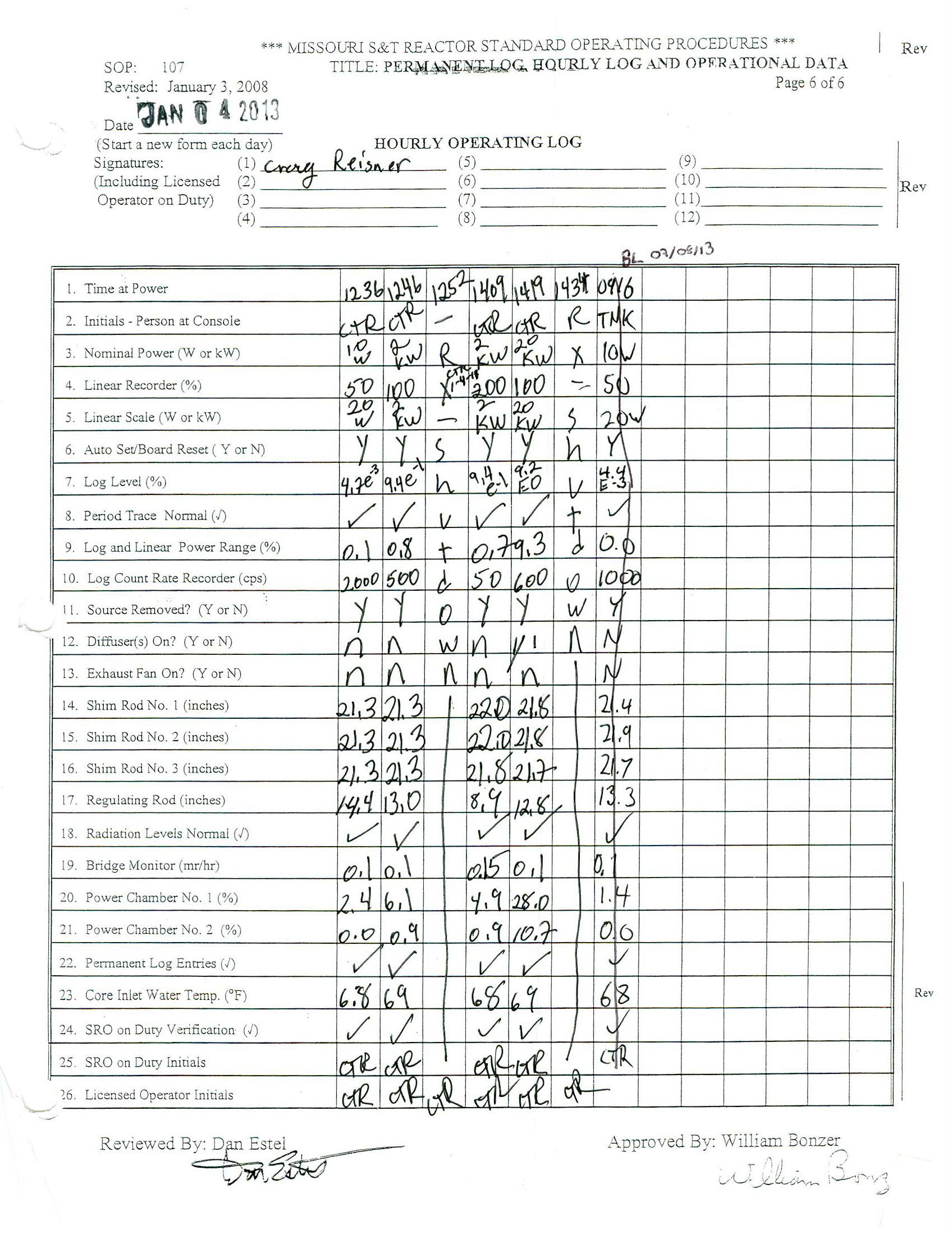
Figure 1: Example MSTR Transient log

The same information was collected from each stable power, with two stable powers forming a single observation for the state-based prediction model. The information from any given stable power could be coupled with the previous or subsequent information from a stable power to create a single data point. The information collected from each of these points included the stable power, control rod heights, date, and time.

Data could be collected in this format and exported to an excel file. Each observation included the date, start time, end time, initial power, final power, and initial and final control rod heights. Date and time data were retained for indexing, while the power and control rod information could be used to define the physical state of the reactor system. Transient data ranging from January 7, 2013, to October 10, 2014, was collected and processed by hand in this manner.

Some observations were excluded from the collected data. For example, reactor shutdowns were not included due to the excess negative reactivity in the core, which could result in model memorization of shutdowns or negatively impact performance by preferentially training towards shutdowns. Transients longer than one hour (from start to finish) were excluded to focus the model on short-term state-based modeling. After data auditing and exclusion, 542 total observations were collected.

Unfortunately, 542 observations would not be enough to adequately train a model. A physical sampling method was implemented to address the challenge associated with inadequate training data. The power defect equation, a generalization of the prompt jump equation, was used to generate these additional samples Lamarsh et al. (2001). This equation is generalized as equation 1. The power defect was applied to the final state in observation to jump from one stable power to another stable power effectively. The power defect method was performed under the condition that the total reactivity change in this state could not exceed 0.5$ and no control rod exceeded the 24 inches of maximum withdrawal. This sampling method could be applied $n$ times and form the bulk of the training data while retaining the actual observations for the testing set. The relationship between the reactor power and reactivity can be expressed by Eq. 1:

$$\frac{P^{+}}{P^{-}}=\frac{1-\rho^{+}}{1+\rho^{-}}$$ (1)

where $\rho^{-}$ is lower reactivity, $\rho^{+}$ is higher reactivity, $P^{+}$ is higher power, and $P^{-}$ is lower power.

A method was defined using python code to randomly perturb control rod heights from both the initial and final state of observation. The functions used to execute this practice are included as 5.1 and 5.2. Both the initial and final states were perturbed by this method to reduce the model’s memorization capabilities. The reactivity was determined using the integral rod worth information for the relevant core configuration based on the date the transient occurred. Over the two years of training samples collected, four different reactor configurations were utilized. The observation date could be cross-referenced to the operational dates of the core configurations to determine which control rod-worth values should be used for the selected sample. For the conversion of the given rod worth values, a delayed neutron fraction ($\beta$) of 0.006 was assumed.

Table 1 represents the relationship between the core configuration and the control rod worths. Using the control rod worths, additional data points could be generated using some random noise. The original and generated datasets can be seen in Figures 2 and 3.

Table 1: Integral Rod Worth for Reactor Core Configurations

Core Configuration	Worth ($)
	Rod 1	Rod 2	Rod 3	Reg Rod
120	6.387	5.380	2.963	0.488
121	6.387	5.380	2.963	0.488
122	6.597	5.398	2.963	0.387
123	6.583	5.267	3.017	0.433

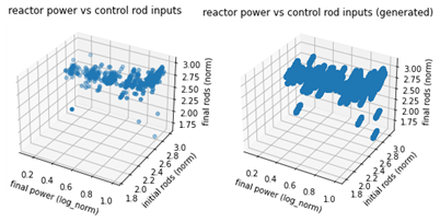
Figure 2: Dataset Distribution (left: original, right: generated)

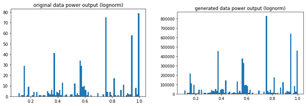
Figure 3: Dataset histograms (left: original, right: generated)

After samples were generated, processing methods could be applied in order to prepare the data for use in deep learning models.

2.2 Pre-Processing

Data pre-processing is required for neural network training methods to ensure a model is effectively trained and allows the model to retain physical significance and interpretability. For the dataset utilized by this model, pre-processing focused on both data normalization and input/ output determination. Normalization improves the way deep neural network models process input information. Determining the best inputs and outputs for a model governs how information is extracted from it. Both normalization and data selection strategies aim to improve the accuracy and efficacy of the model.

2.2.1 Dataset Normalization

The pre-processing procedure primarily centered around normalizing the data set and preparing the target outputs to be used during the training process. A method to normalize a single sample could be developed, extending to the entire dataset, whether actual observation or generated physical sample. Control rod heights were normalized from 0 to 1, with 1 being a full withdrawal of 24 inches. The equation used to normalize control rod height can be seen as equation 2.

$$x_{norm}=x_{rod}/24$$ (2)

Reactor power would need to be normalized and scaled to produce accurate results. To perform this, the natural logarithm of the power was calculated and then normalized to the natural logarithm of full power (200,000 W). The equation used to normalize reactor power can be seen as equation 3.

$$P_{norm}=ln(P)/ln(200,000)$$ (3)

The single observation normalization method is included as 5.3. This method could then be applied to the entire dataset to form the input data of the deep learning model. The equations used in the normalization process are shown below.

The target outputs could then be generated for the model. With a classification scheme, a series of bins could be used to determine the output. Each bin’s ceiling was predefinedpre-defined to best separate the data. Since outputs tended to cluster around exponentials, the classification method would have to be designed such that similar power changes were still grouped together. The classification categories can be seen in Table 2.

Table 2: Original Dataset 5-class Output Distribution

Bin #	0	1	2	3	4
Ceiling (W)	90	900	9000	90000	200000
# of samples	73	94	100	126	149

If all samples were properly classified, undersampling methods could be used. Undersampling is important for models which might have much more of one output than another. The model could preferentially select the more populated class resulting in underfitting. An undersampling method was applied to the generated dataset such that all output classes would have the same number of samples. The undersampling method is included as 5.4.

2.2.2 Input Selection

After data was generated and normalized, the ideal inputs and outputs could be determined. This was primarily performed by analyzing the physical significance of the variables and determining the best separation methods. Using a state-based classifier, the input variables could be mapped to see the target class before they are used to train the model. Plotting the different variables against each other could show which variables have the most significant separation for the classification method.

Different input variables were posed and compared based on their physical significance. Due to the state-based nature of the network, information from both the initial state and final state would need to be used. From both of these states, control rod positions were available. Control rods are the primary governor of reactivity changes in the system, resulting in those variables being a good choice. With the integral rod worth known, the approximate reactivity contribution from rod withdrawal could also be estimated. Using control rod heights as an input variable, a model could learn the physical properties of the reactor internally. This could result in a model which predicts a final power state by processing control rod heights information about the physical state of the reactor. Alternatively, by using the reactivity insertion provided by the control rod heights, the model could predict the state by attempting to model an equation for reactor power directly. Another possible input option was initial power. The normalized initial power would be input and could be used by the model to generate an image of the system’s initial state. This would also allow the model to generate ’jumping off points’ from the common starting states of the reactor. This is due to reactor operators preferentially reaching whole numbers and multiples of 10 when conducting a power change. It could help by clustering the input information with other similar samples.

Along with the clustering from initial power, the direction of change could also be input. Although the model would hopefully use the differences between initial and final states to predict what the power would be internal, providing information about whether a power increase or decrease is performed could help with clustering. This could also be paired with the initial power, which would further reinforce the helpful clusters. For instance, accuracy could be increased by grouping power increases starting at 2 kW separately from power decreases starting at 2 kW. These inputs could be created and separated quickly from the generated dataset and then used to train the deep learning models.

The datasets split into classes plotted against the relevant input variables can be seen in Figure 4 and Figure 5.

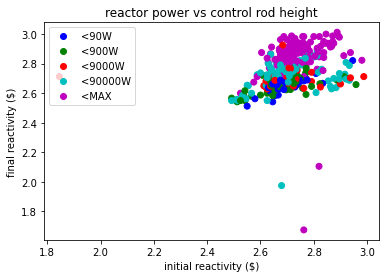
Figure 4: Classification: Reactor power versus rod heights

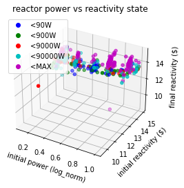
Figure 5: Classification: Reactor power versus reactivity from rods

2.2.3 Neural Network Design

Multiple deep learning models were generated and trained to determine the best design for predicting energy output. The basic type of network used was a feedforward model, although different ways to input the data and internal structures were tested. Regularization methods were deployed in every model to reduce overfitting, with L1 and L2 regularization commonly used. Models were optimized using either the Adam or Stochastic Gradient Descend (SGD) algorithms. The first models generated were classification networks using categorical cross-entropy loss due to the classified nature of the model. All models were designed using the Keras package of the TensorFlow Python module and trained against the generated data set. In contrast, the actual collected data was retained as the testing set.

33% of training samples were retained for a check set for each model. The check dataset was retained to ensure effective training of the model. Specifically, the check set would be run through the model at the end of each epoch. This is so that the neural network will not memorize the original dataset, avoiding overtraining. This standard ML checking method from neural network design is assumed to be an effective training method in this scenario.

An early stopping criterion was also developed for the model to reduce overfitting. If a model’s accuracy did not improve 0.5% within five epochs, then it would stop training and restore itself to the state it was in when it performed the best. TensorFlow performed this by allowing the model to restore its best weights. The model would train for 1000 epochs if this criterion were never achieved. Data were shuffled before each training cycle.

Different models were designed to determine which method would best facilitate the data. This could be typically grouped into two categories: separated input and all-in-one (AIO) input. The AIO input models were formatted like a standard feedforward deep neural network. The input data could be concatenated into a single vector which could be processed by the model for an output. The separated input models attempted to retain some of the physics of the system by having a defined input and output state, which could be processed and then concatenated deeper into the model to be processed for output. A few network designs are included as appendices 5.5 and 5.6. In these figures, the paired numbers indicate the size of that layer. The question mark is an artifact from the plotting functions in TensorFlow, indicating that the input dimension could be variable. The second number in the pair indicates the output size of the layer, pre-defined by the architecture. This is true for all subsequent model architecture plots.

The data input to some models was different from others. Some models used control rod heights as inputs, while some used total reactivity generated by control rods. Some models reduced the total number of input variables by summing the control rod information (when relevant) into a single variable. If the control rod heights were used this way, only control rods 1, 2, and 3 were summed. If the reactivity provided by each control rod was used, all of the rods were summed into a single variable. The types of models designed and trained can be viewed in Table 3.

Table 3: Types of Classifier Models Trained

Model	Separated Input	AIO	Uses Rod Heights	Uses Reactivity	Direction
(a1)	✓			✓	✓
(b1)	✓		✓		✓
(c1)	✓			✓
(d1)	✓		✓
(e1)		✓		✓	✓
(f1)		✓	✓		✓

To make a final prediction, regression models were created. The probabilistic output of the classifier networks could form a basis to better distribute the output values in a regression model and as such, were used as an input. These models utilized a sigmoid output function to squash the output so it could not produce a value greater than 1, which is the normalized maximum power. The architectures were designed similarly to the classifier models, with some having AIO input while others had split input and internal hidden layers. These models were also designed as feedforward neural networks using backpropagation. In both cases, the 5-label output vector from a classifier was used as an additional input. The two general styles are shown in appendices 5.7 and 5.8, along with the types of models produced in Table 4. All regression models utilized the power change direction. All regression models utilized a mean absolute error loss function.

Table 4: Types of Regression Models Trained

Model	Separated Input	AIO	Uses Rod Heights	Uses Reactivity
(a2)	✓		✓
(b2)	✓			✓
(c2)		✓	✓
(d2)		✓		✓

The model designs proposed in this paper follow the basic framework of feedforward deep neural networks using backpropagation. The complete models are proposed to function in series, in which the results from the classification models feed an additional input similar to keyword inputs from the traditional neural network design. Feedforward models’ benefit is their generalization ability and low computational resource requirements. The goal of these model designs was to allow for short-term forecasting during power change operations, which could assist reactor operators and allow for operational changes if necessary. Functions were created so each model could be quickly initialized. Once the data set was loaded and the model was initialized, each could be trained.

3 RESULTS & DISCUSSIONS

After models were created and inputs were generated, the proposed framework could be used in power prediction. The following sections show the training and testing results, with the results graphed for ease of visualization.

3.1 Training

The table below shows the models trained and relevant variables associated with their training. Models were stopped early if the aforementioned early stopping criterion was met. If a model were stopped this way, it would revert to the epoch in which it had the highest validation accuracy. Table 5 includes information from these epochs.

Table 5: Trained models and relevant variables

Model	Total Epochs	Best Validation Loss	Best Validation Accuracy
(a1)	15	0.3711	0.8568
(b1)	11	0.4697	0.8214
(c1)	11	0.3536	0.8708
(d1)	13	0.4829	0.8194
(e1)	6	0.9092	0.6549
(f1)	9	0.9093	0.6433

The loss and accuracy metrics of the models trained are included as Figures 6 and 7. A history of the training cycle was retained for this purpose. Figure 6 depicts the training losses of each model per epoch of training, and figure 7 depicts the accuracy of each model per epoch trained. This can be used to determine how quickly and effectively the models are trained. High performance models were saved in case they would need to be loaded in future instances.

It can be seen that while the split-input type models performed well, the AIO input models trained poorly. This is likely due to a lack of feature separation, causing confusion in the model. This would imply that input separation improves training for a physical problem.

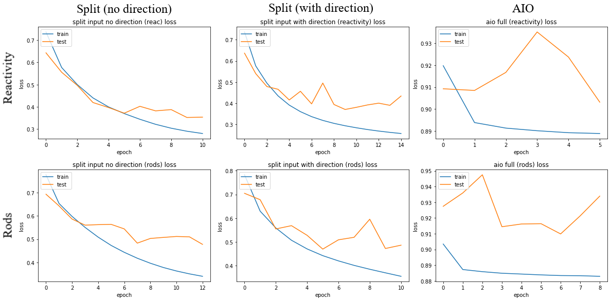
Figure 6: Classifier training losses

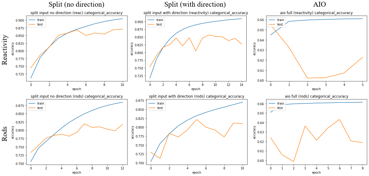
Figure 7: Classifier training accuracies

Regression models were trained using the output from the classifier most closely resembling its input. Early stopping criteria were applied, with the AIO regression predictors monitoring mean squared error and split input predictors monitoring loss. Models could be tested with the retained data after they were trained. The data from the regression predictor early stopping is included in Table 6.

Table 6: Regression predictor training

Model	Total Epochs	Best Validation Loss	Best Validation Accuracy
(a2)	14	0.0646	0.0082
(b2)	16	0.0559	0.0059
(c2)	6	0.0621	0.0082
(d2)	7	0.0541	0.0060

3.2 Verification

The testing results are included below. The goal of the testing is to verify that the models are capable of effective utility in MSTR. It is split into a section for the classifier and regression models.

3.2.1 Classifiers

After training, the better-performing models could be tested with the actual data from the reactor. Data from the reactor could be formatted into vectors and used by the model to predict outputs. Confusion matrices were used to visualize how well the data performed on the original dataset. The result is shown in Figure 8.

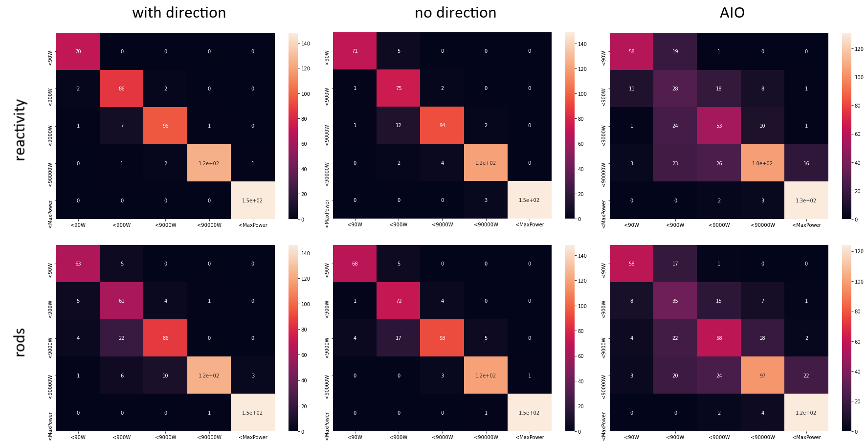
Figure 8: Confusion matrices from actual dataset

Precision and recall of the models could also be calculated to determine the best performers.

Table 7: Macro F1 scores of models

Model	Accuracy	Macro F1
(a1)	0.969	0.966
(b1)	0.886	0.874
(c1)	0.941	0.936
(d1)	0.924	0.918
(e1)	0.692	0.667
(f1)	0.686	0.673

It can be seen that the reactivity models produced better results than the rod height models. The internal accuracy metrics of some of the models are listed in Tables 8, 9, and 10.

Table 8: Internal accuracy metrics of model a1

Class	Precision	Recall	F1
<90W	1.000	0.959	0.979
<900W	0.956	0.915	0.935
<9000W	0.914	0.960	0.937
<90000W	0.969	0.992	0.980
<MAX	1.000	0.993	0.997

Table 9: Internal accuracy metrics of model d1

Class	Precision	Recall	F1
<90W	0.932	0.932	0.932
<900W	0.935	0.766	0.849
<9000W	0.782	0.93	0.849
<90000W	0.968	0.952	0.960
<MAX	0.993	0.993	0.993

Table 10: Internal accuracy metrics of model e1

Class	Precision	Recall	F1
<90W	0.744	0.795	0.768
<900W	0.424	0.298	0.350
<9000W	0.596	0.530	0.561
<90000W	0.607	0.833	0.702
<MAX	0.963	0.879	0.919

3.2.2 Regression

The regression models were trained using the output from the classifier most closely resembling its input type. The distribution and error of the regression models can be analyzed to show their efficacy. The results are shown in Figures 9, 10, and 11.

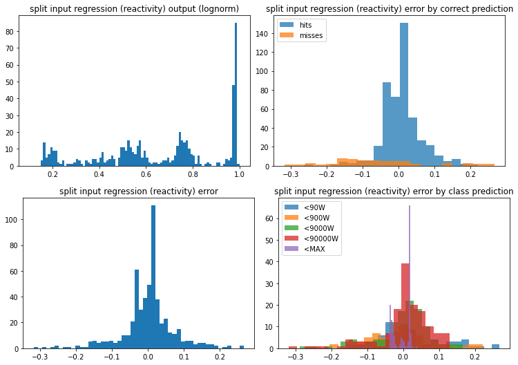
Figure 9: a2 prediction error

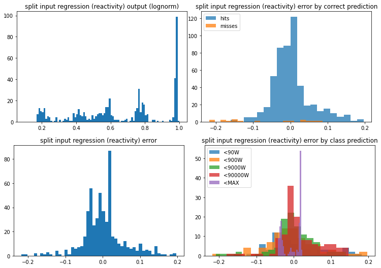
Figure 10: b2 prediction error

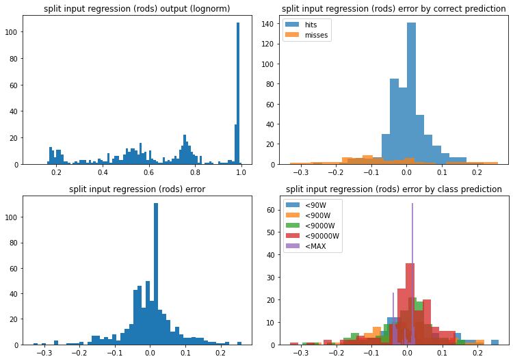
Figure 11: c2 prediction error

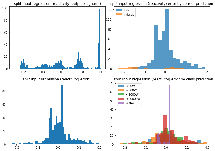
Figure 12: d2 prediction error

The results show that the models using control rod height rather than reactivity have a blind spot around the 0.4 output spike in the original dataset. This could be due to either the worse performance of the first stage classifiers using control rod height or the model cannot correctly infer the reactor physics from the control rod heights. The AIO and split input models have only minimal difference between the two, implying that most of the prediction information is inferenced from the classifier from the previous stage. Additional regularization of the classification input could help reduce this reliance.

3.2.3 Combined Model

To complete the model, the most successful models from each stage can be combined. A model can be defined in Tensorflow using a trained model from each stage as a functional layer. The result is a model which takes the input utilized in the first stage of the model and internally processes it for use in the second stage of the model. The output of the first stage is also utilized for the input in the second stage, as outlined in the training section. The full model with two functional layers and an input layer can be seen in Figure 13. The selected first-stage model was a1, and the selected second-stage model was b2.

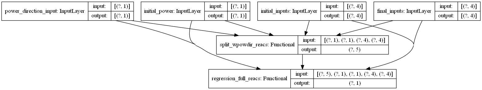
Figure 13: Final two-stage model

The resultant DNN outputs both categorical and numerical predictions. Since DNNs are replicable, the predictions in each stage are the same as those from models a1 and b2. This final DNN can be functionally applied, retrofitted, and exported to function as a component in a larger system.

Practically, a similar type of model could likely be developed in other reactors. The inputs would have to be developed based on the design of the reactor core, and the inputs could further be expanded as well. The normalization of control rod heights could cause the reduced accuracy of the models using control rod heights as input. More likely, however, is that the models struggle to inference the physics of the reactor core. With the reactivity provided, the model does not have to infer the effect of the rods on the power but can directly map the reactor power to reactivity. This allows future models to account for negative reactivity provided by burnable poisons or testing samples. Furthermore, reactivity would also allow the model to be more useable on reactor core configurations it was not trained on. That said, classifier accuracy for control rods could have been more impractically high, and most incorrect predictions were in an adjacent energy resolution. The classification accuracy using control rods is at least a proof of concept for future models using similar inputs.

Over the time the data was collected, MSTR saw significant use. This could have led to changes in core physics. This time period corresponds to a total burnup of 120MWd/MTU. Based on the fuel designs, this is 13% of the fuel’s lifetime burnup. This physical change, along with the increase of poisons generated inside the fuel, could cause complications with the results. Additional support modules may need to be developed to account for these effects.

4 CONCLUSIONS

Of the models generated, the classifier models produce effective results. Since the softmax output function is probabilistic, the outputs can be more closely reviewed to determine whether they are useable. The reactivity models provided by control rods produced more reliable results than those utilizing control rod heights. In a practical situation, reactivity input should be used for a predictive model if available. The power change direction provided only a minor change in the accuracy of the classifier. It could be excluded if desired.

The regression models produced reliable results as well. Accurate classifier predictions tended to remain within 10% error, although the prediction error would be much larger, closer to 1, due to the log normalization methods. In the regression models, the control rods also produced worse results than the reactivity states. Incorrect predictions, in general, could reach 20% error, likely due to the clustering around the 2*10x power states.

This implies that with robust analysis, a multi-stage machine learning model using probabilistic-to-continuous conversion would be useful in a DT system. This type of model effectively improves the reliability of predictions when the classification is correct, which can be analyzed in other subsystems or by personnel. This information can be used in other models, and uncertainty analysis can be performed using both prediction aspects of the model. These models are also computationally cheap after training, which is important for DT components.

Future work will take two forms; improved data and continued development. Increasing the available data would be useful, but more specifically, increasing the available input features and generating more distributed data would yield better results. Since the power output clusters around the 2*10x powers, the regression model can rely heavily on the classifier output. More distributed power output could force the regression network to train more using the physical information from the reactor. Additional input information could also be useful, such as the total reactor uptime, the presence of a sample, burnable poison, etc. Additional input features could affect accuracy.

The other subject of future research would be continued development. Besides developing different architectures for testing, the logical next steps would be either a full predictor, modular controller, or both. A Long Short-Term Memory (LSTM) or convolutional neural network could be developed as a time series predictor. A state-based predictor like the one developed could be used in conjunction with this model, which would provide an end state as a horizontal asymptote for the time series. If this type of model was desired, the state-based model could also be modified to produce a value for the time required to reach the final power as well. If an automatic controller were desired, one could be developed in conjunction with a state-based predictor as a sort of look-ahead function. The controller would perform an action, and the predictor could generate the final power of the transient and provide feedback to the controller. In fact, using a similar model to approximate feedback terms from reactor operation could be used in conjunction with other types of models (machine learning or physics-based) to streamline the prediction process. The predictor-controller could then be modularized and actively receive live information from the reactor to form an online automatic controller.

Furthermore, continued development will be performed to realize practical applications as a module in the back end of a Digital Twin (DT) system. Since DTs seek to give real-time data and system state predictions, this model could easily be implemented to generate those short-term predictions. This would allow operators or other modules to use control rod information to make decisions minutes to hours in advance. As DT research and applications become more popular ultra-lightweight predictive tools such as this will be an important part of the design process, allowing the advanced models to have a physics-based real-world rooting.

5 APPENDIX

5.1 power_ratio_sample function

⬇

1# creates an additional datapoint from sample

2# uses power ratio for small reactivities

3# equation from Lamarsh 346-347

4# performes microscopic power change on previously existing sample

5# assume given 4 rods and reactivities

6# allows additional preturbation of regulating rod (pos4)

7def power_ratio_sample(rods, power, reacs, change):

8 # determines whether the additional power change is positive or negative

9 # mainly changes the behavior of the random number generator

10 clear=False

11 delta = np.random.normal(loc=0.0, scale=0.15, size=4)

12 if change==1:

13 delta[0] = delta[0]+0.3

14 delta[1] = delta[1]+0.3

15 delta[2] = delta[2]+0.3

16 if change==-1:

17 delta[0] = delta[0]-0.3

18 delta[1] = delta[1]-0.3

19 delta[2] = delta[2]-0.3

20 if change==0:

21 delta[0] = (delta[0])

22 delta[1] = (delta[1])

23 delta[2] = (delta[2])

24 # preturb regulating rod separately

25 delta[3] = delta[3]*10

26 new_rods = delta+rods

27 # check if all control rod heights are real

28 if np.max(new_rods)>24 or np.min(new_rods)<0:

29 clear=False

30 else:

31 clear=True

32 # determine initial reactivity

33 init_reacs = rods*reacs

34 reac_i = np.sum(init_reacs)

35 # determine change in reactivity

36 delta_reacs = new_rods*reacs

37 reac_f = np.sum(delta_reacs)

38 # determine micro power change

39 new_power = power*((1-reac_f)/(1-reac_i))

40 # catch overpowers

41 if new_power>200000:

42 clear=False3

43 # equation becomes invalid for reactivities larger than 0.5$

44 if abs(reac_f-reac_i)>0.5:

45 clear=False

46 # outputs new rod and power state

47 return new_rods, new_power, clear

5.2 over_sample function

⬇

1# creates additional samples en masse

2# integral reactivity represented in $

3def over_sample(dataset, dates, n, change):

4 # create new array for generated data

5 new_data = np.empty(shape=(n,11))

6

7 # reactivities of each core configuration

8 reacs120 = np.array([.03832, .03228, .01778, .00293])/0.006

9 reacs121 = np.array([.03832, .03228, .01778, .00293])/0.006

10 reacs122 = np.array([.03958, .03239, .01778, .00232])/0.006

11 reacs123 = np.array([.0395, .0316, .0181, .0026])/0.006

12 # start dates of each core configuration, in ordinal

13 core121=date(year=2014, month=1, day=15)

14 core121=int(core121.toordinal())

15 core122=date(year=2014, month=10, day=9)

16 core122=int(core122.toordinal())

17 core123=date(year=2014, month=10, day=16)

18 core123=int(core123.toordinal())

19

20 # generate new samples via power ratio

21 for i in range(n):

22 # determine which original sample to use

23 og = np.random.randint(low=0, high=dataset.shape[0])

24 power_i = dataset[og,0]

25 power_f = dataset[og,1]

26 rods_i = dataset[og,2:6]

27 rods_f = dataset[og,6:10]

28 date_code = dataset[og,10]

29 # get the reactivity for this power change

30 day = dates[og]

31 if day<core121:

32 reacs=reacs120

33 config = 0

34 elif day<core122:

35 reacs=reacs121

36 config = 1

37 elif day<core123:

38 reacs=reacs122

39 config = 2

40 else:

41 reacs=reacs123

42 config = 3

43 # generate new initial state

44 new_rods_i, new_power_i, pass_i = power_ratio_sample(rods_i, power_i, reacs, change)

45 # generate new final state

46 new_rods_f, new_power_f, pass_f = power_ratio_sample(rods_f, power_f, reacs, change)

47 # port new information to output array

48 new_data[i,0] = new_power_i # initial power

49 new_data[i,1] = new_power_f # final power

50 new_data[i,2:6] = new_rods_i # initial rod heights

51 new_data[i,6:10] = new_rods_f # final rod heights

52 new_data[i,10] = date_code # ordinal date

53 # if sample doesn’t pass, redo sample

54 if not(pass_i) or not(pass_f):

55 i=i-1

56 return new_data

5.3 normalize_sample function

⬇

1# normalizes one sample for input to models

2def normalize_sample(sample, y):

3 # normalize inputs

4 output = np.empty(shape=(np.shape(sample)))

5 output[0] = np.log(sample[0])/np.log(200000) # gets log of initial power

6 output[1] = np.log(sample[1])/np.log(200000) # gets log of final power

7 output[2:6] = sample[2:6] / 24 # normalizes control rod height to max withdrawal

8 output[6:10] = sample[6:10] / 24 # normalizes control rod height to max withdrawal

9 output[10] = sample[10]

10 # normalize outputs

11 y_out = np.empty(shape=(np.shape(y)))

12 y_out[0] = y[0]

13 if y[1]<0:

14 out = np.abs(y[1])

15 out = np.log(out)

16 out = -out

17 y_out[1] = out

18 else:

19 out = y[1]

20 out = np.log(out)

21 y_out[1] = out

22 return output, y_out

5.4 undersample_from_sorted function

⬇

1# takes sorted array and undersamples so that each class has an even number of samples

2def undersample_from_sorted(sorted_list):

3 # get number of samples in each class

4 classes = len(sorted_list)

5 count=[]

6 # make empty arrays for counts in each class and counts for porting

7 for i in range(classes):

8 count.append(0.0)

9 # get number of samples in each class

10 for i in range(classes):

11 count[i] = sorted_list[i].shape[0]

12 # determine shape of new array

13 features = sorted_list[0].shape[1]

14 size = min(count)

15 smallest = count.index(min(count))

16 undersampled = np.empty(shape=(size*classes,features))

17 # loop through each class

18 index_count = 0

19 for i in range(classes):

20 # port smallest class directly

21 if i==smallest:

22 for j in range(size):

23 undersampled[index_count,:] = sorted_list[i][j,:]

24 index_count+=1

25 # random sample the other classes

26 else:

27 samples = sorted_list[i].shape[0]

28 for j in range(size):

29 # get random sample from desired class

30 current = np.random.randint(0,samples-1)

31 undersampled[index_count,:] = sorted_list[i][current,:]

32 # count up

33 index_count+=1

34 return undersampled

5.5 Multi-input Classifier Model (with Power Change Direction)

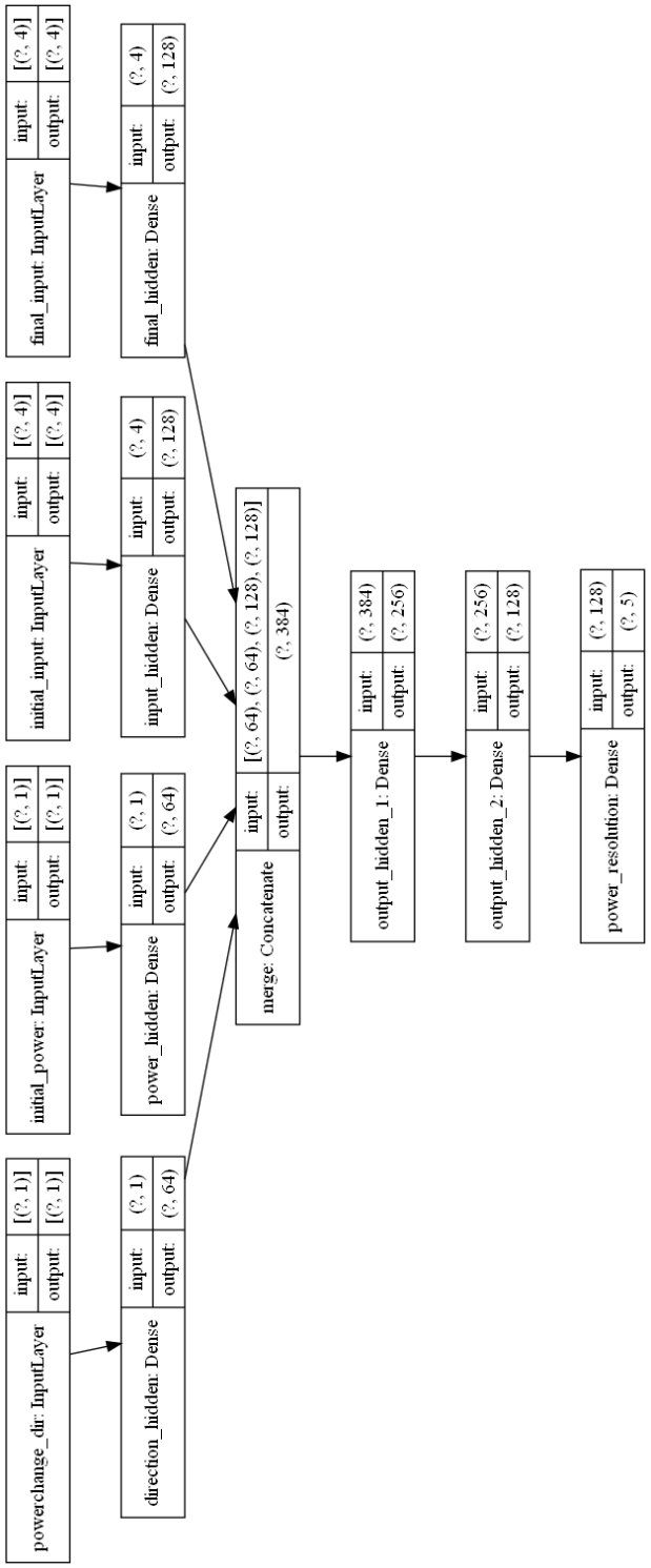
Figure 14: Graphical representation of classifier neural network utilizing separated inputs, including direction of power change. Figure generated through GraphViz and Tensorflow.

5.6 All-In-One Classifier Model

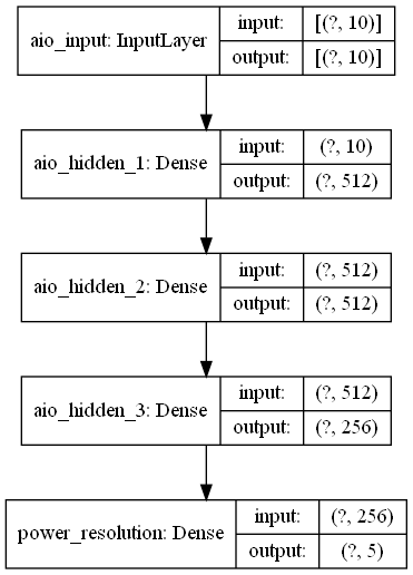
Figure 15: Graphical representation of classifier neural network utilizing all-in-one inputs. Data is concatenated in the first layer and processed at once. Figure generated through GraphViz and Tensorflow.

5.7 Split-input Regression Model

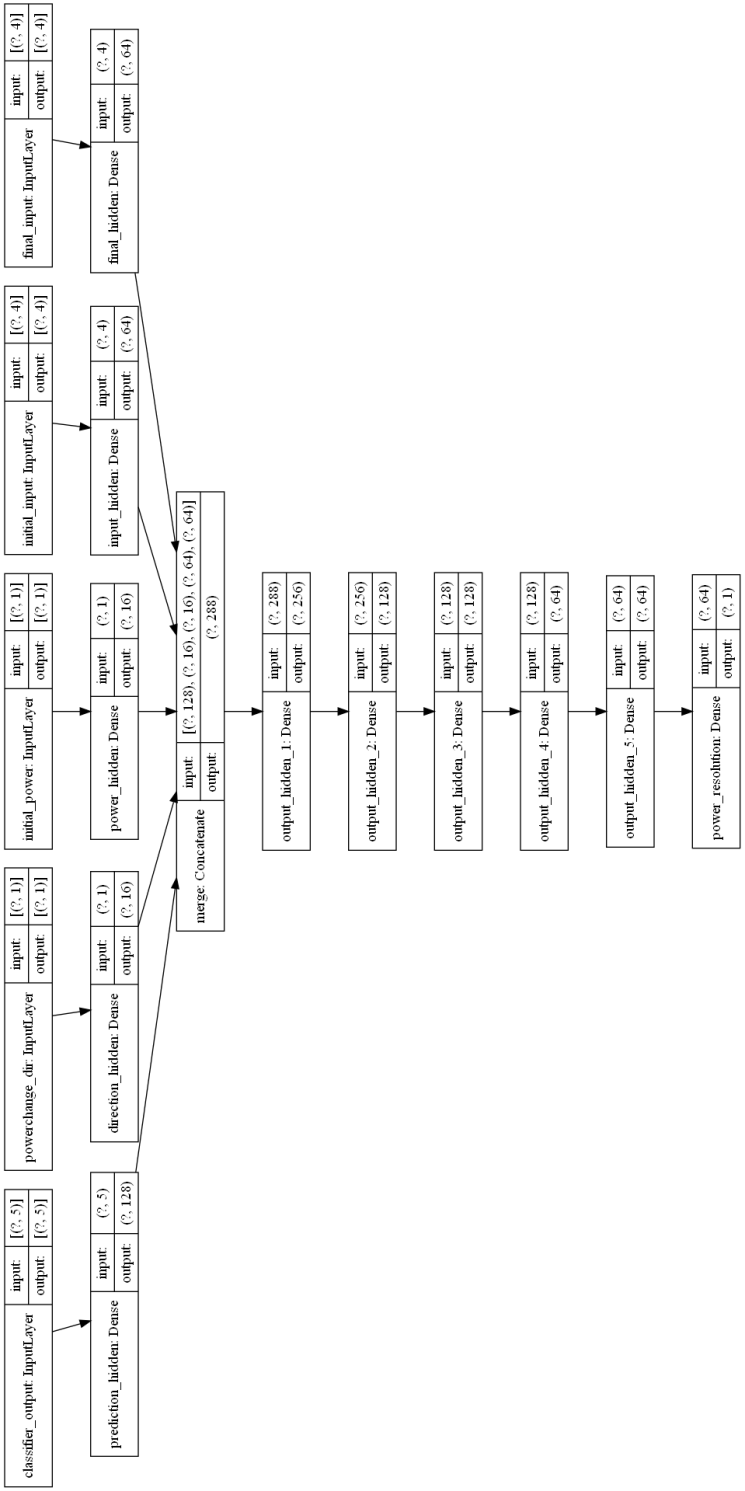
Figure 16: Graphical representation of regression model using split inputs. Input includes standard inputs for classifier model and probabilistic vector of output ranges. Figure generated through GraphViz and Tensorflow

5.8 All-In-One Regression Model

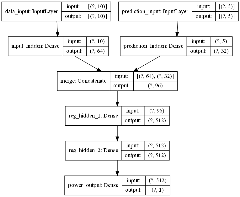
Figure 17: Graphical representation of regression model using all-in-one input. Input includes concatenated data vector and a separate probabilistic input for ranged generated by the classifier. Figure generated through GraphViz and Tensorflow

References

- Samal and Ghosh [2020] Kumar Samal and Suman Ghosh. Characterization and prediction of flow-conditions in the hot-leg of pwr during loss of coolant accident. Nuclear Engineering and Design, 359:110446, 2020.
- Okita et al. [2019] Taira Okita, Tomoya Kawabata, Hideaki Murayama, Nariaki Nishino, and Masaatsu Aichi. A new concept of digital twin of artifact systems: Synthesizing monitoring/inspections, physical/numerical models, and social system models. Procedia CIRP, 79:667–672, 2019. ISSN 22128271. doi:10.1016/J.PROCIR.2019.02.048.
- Varé and Morilhat [2020] Christophe Varé and Patrick Morilhat. Digital twins, a new step for long term operation of nuclear power plants. Lecture Notes in Mechanical Engineering, pages 96–103, 2020. ISSN 21954364. doi:10.1007/978-3-030-48021-9_11/FIGURES/4. URL https://link.springer.com/chapter/10.1007/978-3-030-48021-9_11.
- Sleiti et al. [2022] Ahmad K. Sleiti, Jayanta S. Kapat, and Ladislav Vesely. Digital twin in energy industry: Proposed robust digital twin for power plant and other complex capital-intensive large engineering systems. Energy Reports, 8:3704–3726, 11 2022. ISSN 23524847. doi:10.1016/J.EGYR.2022.02.305.
- Erol et al. [2020] Tolga Erol, Arif Furkan Mendi, and Dilara Dogan. Digital transformation revolution with digital twin technology. 4th International Symposium on Multidisciplinary Studies and Innovative Technologies, ISMSIT 2020 - Proceedings, 10 2020. doi:10.1109/ISMSIT50672.2020.9254288.
- Bowman et al. [2022] David Bowman, Lynn Dwyer, Andrew Levers, Eann A. Patterson, Sally Purdie, and Konstantin Vikhorev. A unified approach to digital twin architecture-proof-of-concept activity in the nuclear sector. IEEE Access, 10:44691–44709, 2022. ISSN 21693536. doi:10.1109/ACCESS.2022.3161626.
- Lin et al. [2020] Linyu Lin, Han Bao, and Nam Truc Dinh. On the formalization of development and assessment process for digital twins reactor safety development programme (rsdp) in vietnam view project computationally efficient prediction of containment thermal hydraulics using multi-scale simulation view project. 2020. doi:10.13182/T123-33488. URL https://dx.doi.org/10.13182/T123-33488.
- Kochunas and Huan [2021] Brendan Kochunas and Xun Huan. Digital twin concepts with uncertainty for nuclear power applications. Energies 2021, Vol. 14, Page 4235, 14:4235, 7 2021. ISSN 1996-1073. doi:10.3390/EN14144235. URL https://www.mdpi.com/1996-1073/14/14/4235/htmhttps://www.mdpi.com/1996-1073/14/14/4235.
- Massaoudi et al. [2021a] Mohamed Massaoudi, Ines Chihi, Haitham Abu-Rub, Shady S Refaat, and Fakhreddine S Oueslati. Convergence of photovoltaic power forecasting and deep learning: State-of-art review. IEEE Access, 2021a.
- Demuth et al. [2014] Howard B Demuth, Mark H Beale, Orlando De Jess, and Martin T Hagan. Neural network design. Martin Hagan, 2014.
- Lu et al. [2021] Bi-Liang Lu, Zhao-Hua Liu, Hua-Liang Wei, Lei Chen, Hongqiang Zhang, and Xiao-Hua Li. A deep adversarial learning prognostics model for remaining useful life prediction of rolling bearing. IEEE Transactions on Artificial Intelligence, 2(4):329–340, 2021.
- Leva et al. [2017] Sonia Leva, Alberto Dolara, Francesco Grimaccia, Marco Mussetta, and Emanuele Ogliari. Analysis and validation of 24 hours ahead neural network forecasting of photovoltaic output power. Mathematics and computers in simulation, 131:88–100, 2017.
- Bin and Wenlai [2013] Sun Bin and Yan Wenlai. Application of gaussian process regression to prediction of thermal comfort index. In 2013 IEEE 11th International Conference on Electronic Measurement & Instruments, volume 2, pages 958–961. IEEE, 2013.
- Kim et al. [2014] Dong Yeong Kim, Kwae Hwan Yoo, Ju Hyun Kim, Man Gyun Na, Seop Hur, and Chang-Hwoi Kim. Prediction of leak flow rate using fuzzy neural networks in severe post-loca circumstances. IEEE Transactions on Nuclear Science, 61(6):3644–3652, 2014.
- El-Sefy et al. [2021] M El-Sefy, A Yosri, W El-Dakhakhni, S Nagasaki, and L Wiebe. Artificial neural network for predicting nuclear power plant dynamic behaviors. Nuclear Engineering and Technology, 53(10):3275–3285, 2021.
- Corrado [2021] Jonathan K Corrado. Human-machine system optimization in nuclear facility systems. Nuclear Engineering and Technology, 53(10):3460–3463, 2021.
- Kim et al. [1993] Wan Joo Kim, Soon Heung Chang, and Byung Ho Lee. Application of neural networks to signal prediction in nuclear power plant. IEEE Transactions on Nuclear Science, 40(5):1337–1341, 1993.
- Myung-Sub et al. [1991] Roh Myung-Sub, Cheon Se-Woo, and Chang Soon-Heung. Thermal power prediction of nuclear power plant using neural network and parity space model. IEEE transactions on nuclear science, 38(2):866–872, 1991.
- Zhang et al. [2019] Aoxin Zhang, Jing Teng, Yun Ju, and Rong Zhou. Thermal power prediction of nuclear reactor core based on lstm. In 2019 Chinese Automation Congress (CAC), pages 5303–5307. IEEE, 2019.
- Shouman et al. [2022] Marwa A Shouman, Amany S Saber, Mohamed K Shaat, Ayman El-Sayed, and Hanaa Torkey. A hybrid machine learning model for reliability evaluation of the reactor protection system. Alexandria Engineering Journal, 61(9):6797–6809, 2022.
- Sola and Sevilla [1997] Jorge Sola and Joaquin Sevilla. Importance of input data normalization for the application of neural networks to complex industrial problems. IEEE Transactions on nuclear science, 44(3):1464–1468, 1997.
- Do Koo et al. [2018] Young Do Koo, Man Gyun Na, Kyung-Suk Kim, and Chang-Hwoi Kim. Prediction of nuclear reactor vessel water level using deep neural networks. In 2018 International Conference on Electronics, Information, and Communication (ICEIC), pages 1–3. IEEE, 2018.
- Radaideh et al. [2020] Majdi I Radaideh, Connor Pigg, Tomasz Kozlowski, Yujia Deng, and Annie Qu. Neural-based time series forecasting of loss of coolant accidents in nuclear power plants. Expert Systems with Applications, 160:113699, 2020.
- Massaoudi et al. [2021b] Mohamed Massaoudi, Haitham Abu-Rub, Shady S Refaat, Ines Chihi, and Fakhreddine S Oueslati. Deep learning in smart grid technology: A review of recent advancements and future prospects. IEEE Access, 9:54558–54578, 2021b.
- Hossain et al. [2020] Md Alamgir Hossain, Ripon K Chakrabortty, Sondoss Elsawah, and Michael J Ryan. Hybrid deep learning model for ultra-short-term wind power forecasting. In 2020 IEEE International Conference on Applied Superconductivity and Electromagnetic Devices (ASEMD), pages 1–2. IEEE, 2020.
- Muralitharan et al. [2018] K Muralitharan, Rathinasamy Sakthivel, and R Vishnuvarthan. Neural network based optimization approach for energy demand prediction in smart grid. Neurocomputing, 273:199–208, 2018.
- Lamarsh et al. [2001] John R Lamarsh, Anthony John Baratta, et al. Introduction to nuclear engineering, volume 3. Prentice hall Upper Saddle River, NJ, 2001.