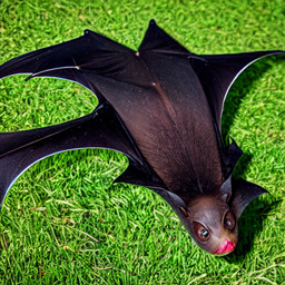
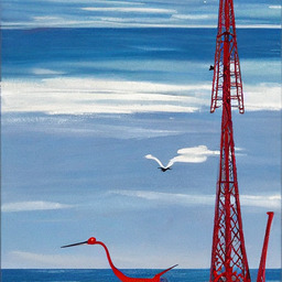
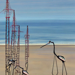
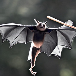
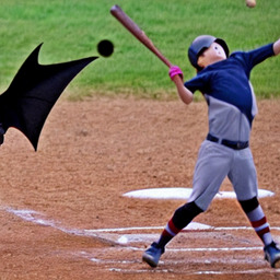
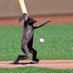
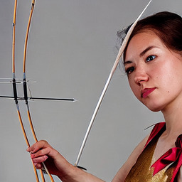
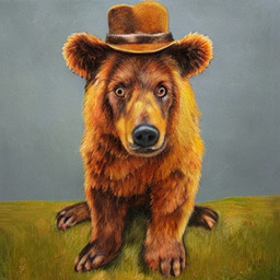
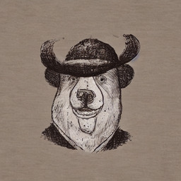
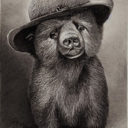
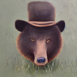
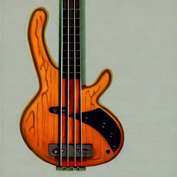
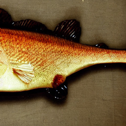
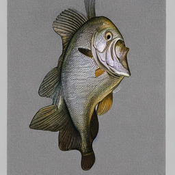
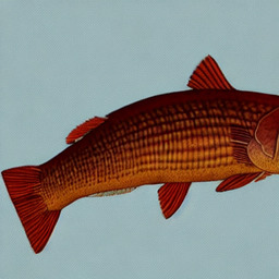
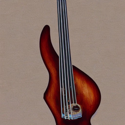
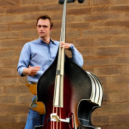
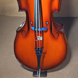
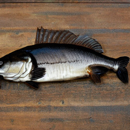
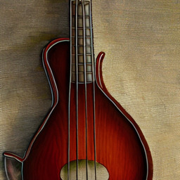
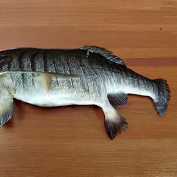
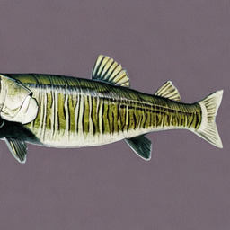
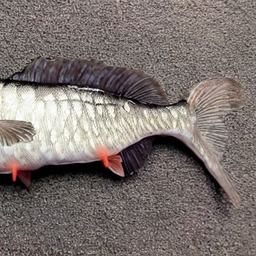
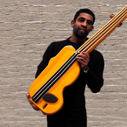
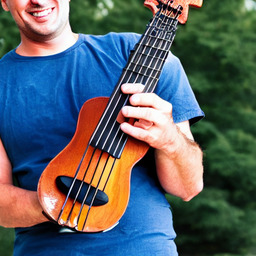
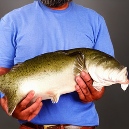
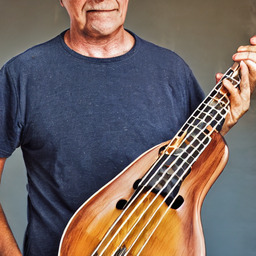
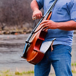
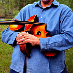
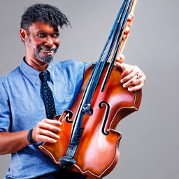
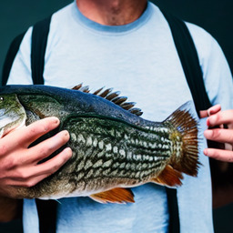
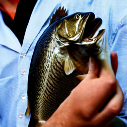
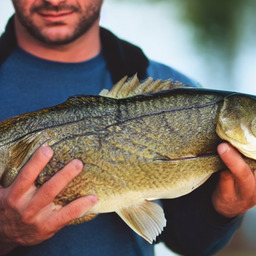
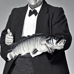
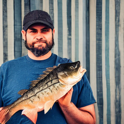
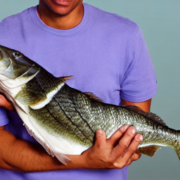
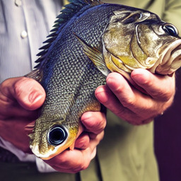
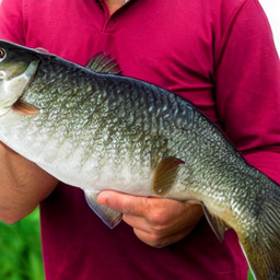
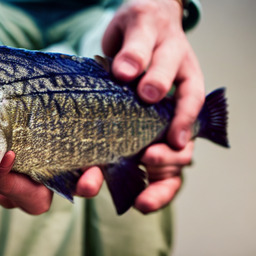
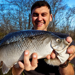
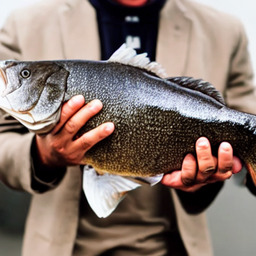
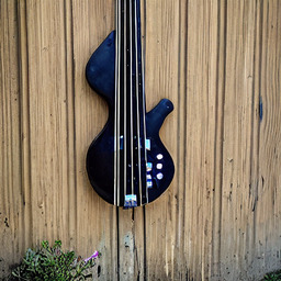
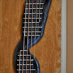
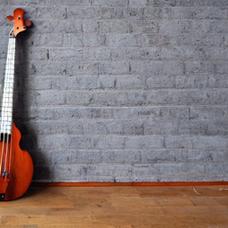
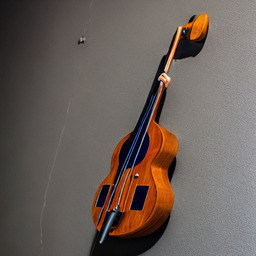
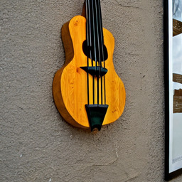
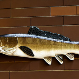
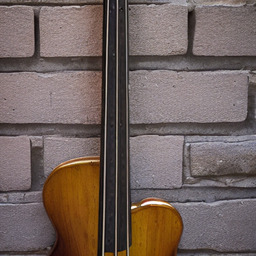
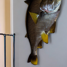
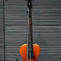
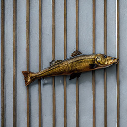
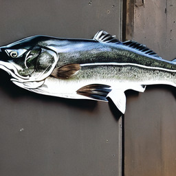
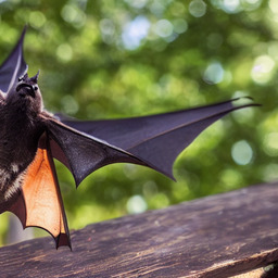
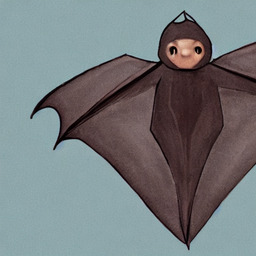
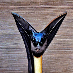
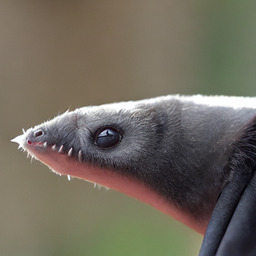
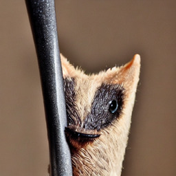
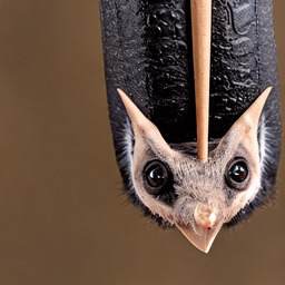
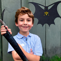
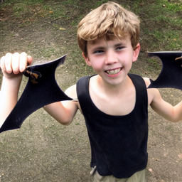
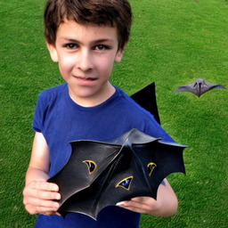
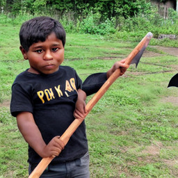
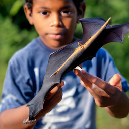
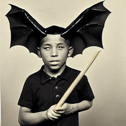
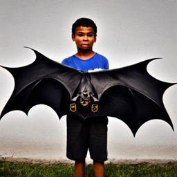
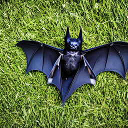
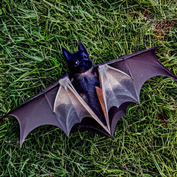
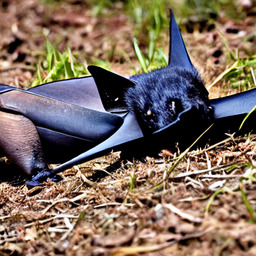
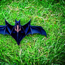
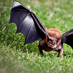
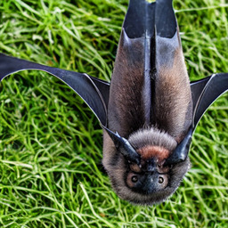
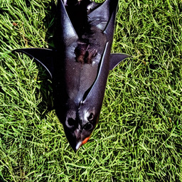
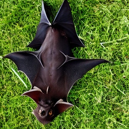
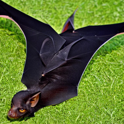
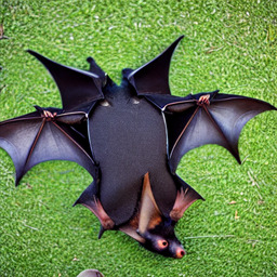
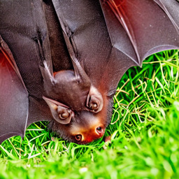
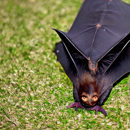
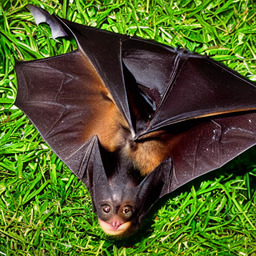
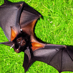
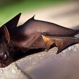
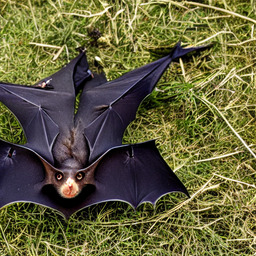
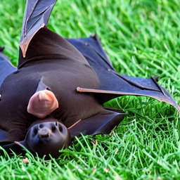
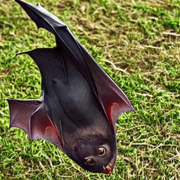
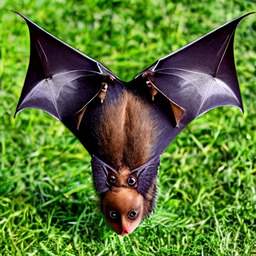
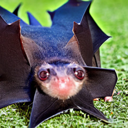
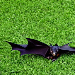
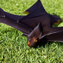
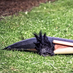
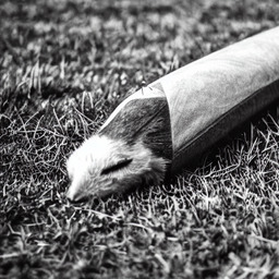
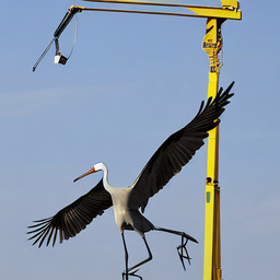
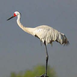
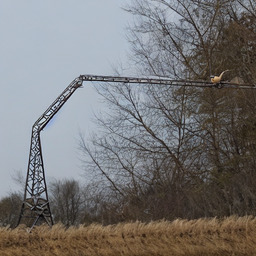
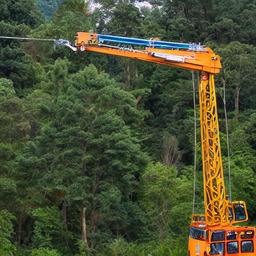
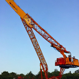
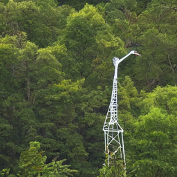
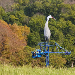
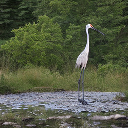
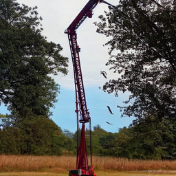
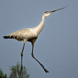
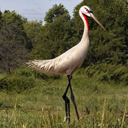
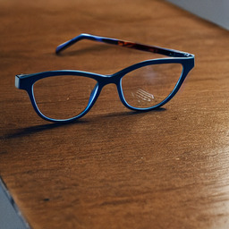
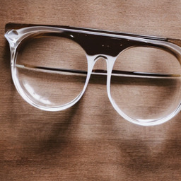
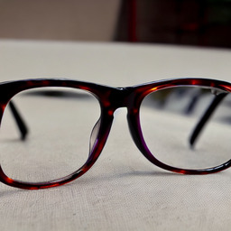
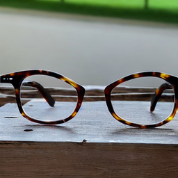
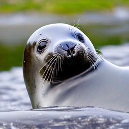
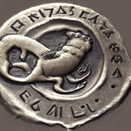
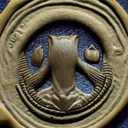
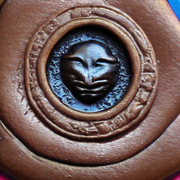
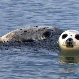
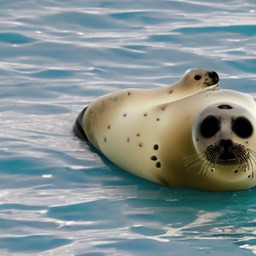
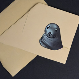
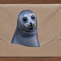
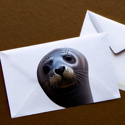
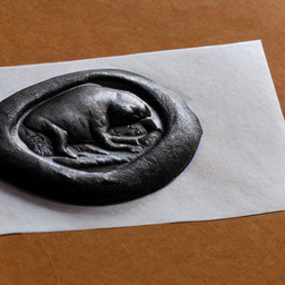
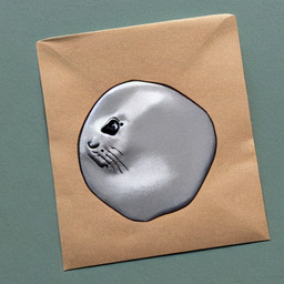
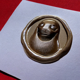
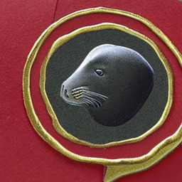
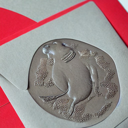
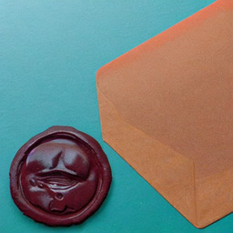
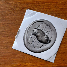
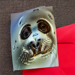
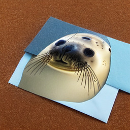
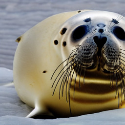
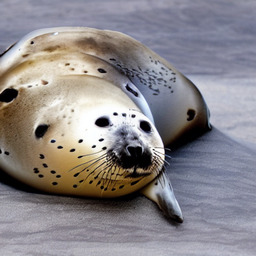
Schrödinger’s Bat: Diffusion Models Sometimes Generate Polysemous Words in Superposition

Jennifer C. White[Uncaptioned image][Uncaptioned image]{}^{\includegraphics[scale={0.05}]{bat_1f987.jpg}}      Ryan Cotterell[Uncaptioned image][Uncaptioned image]{}^{\includegraphics[scale={0.05}]{baseballbat.jpg}}
[Uncaptioned image]University of Cambridge   [Uncaptioned image]ETH Zürich
jw2088@cam.ac.uk   ryan.cotterell@inf.ethz.ch
Abstract

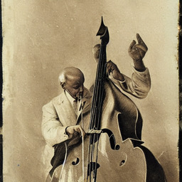
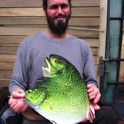
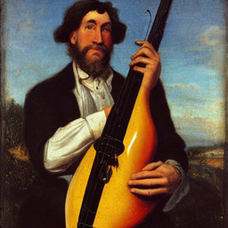
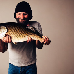
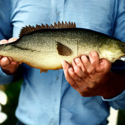
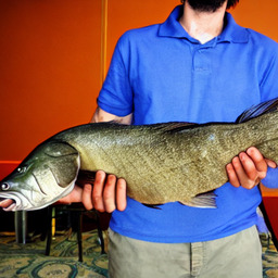
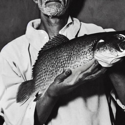
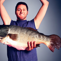
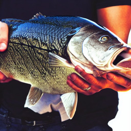
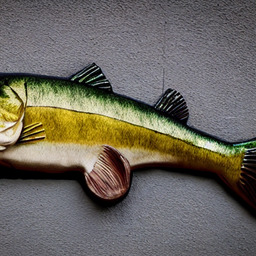
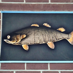
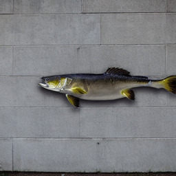
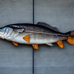
Recent work has shown that despite their impressive capabilities, text-to-image diffusion models such as DALL·E 2 (Ramesh et al., 2022) can display strange behaviours when a prompt contains a word with multiple possible meanings, often generating images containing both senses of the word (Rassin et al., 2022). In this work we seek to put forward a possible explanation of this phenomenon. Using the similar Stable Diffusion model (Rombach et al., 2022), we first show that when given an input that is the sum of encodings of two distinct words, the model can produce an image containing both concepts represented in the sum. We then demonstrate that the CLIP encoder used to encode prompts (Radford et al., 2021) encodes polysemous words as a superposition of meanings, and that using linear algebraic techniques we can edit these representations to influence the senses represented in the generated images. Combining these two findings, we suggest that the homonym duplication phenomenon described by Rassin et al. (2022) is caused by diffusion models producing images representing both of the meanings that are present in superposition in the encoding of a polysemous word.

  [Uncaptioned image]    https://github.com/rycolab/diffusion-polysemy

1 Introduction

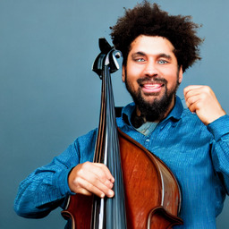
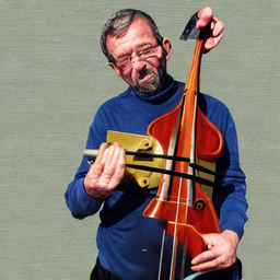
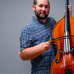
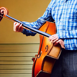
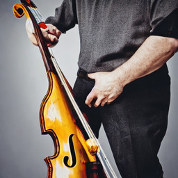
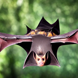
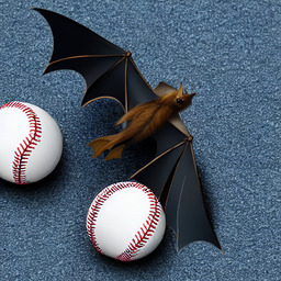
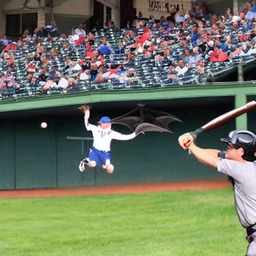
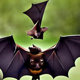
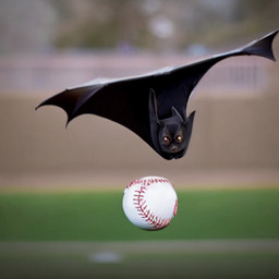
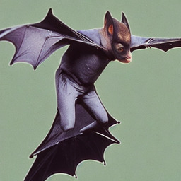
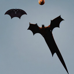
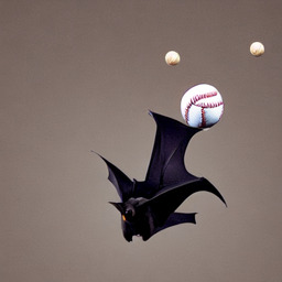
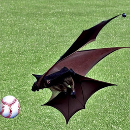
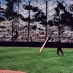
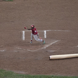
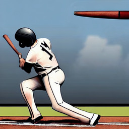
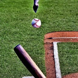
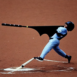
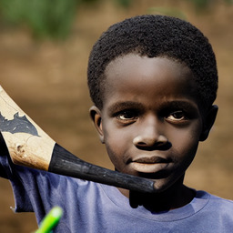
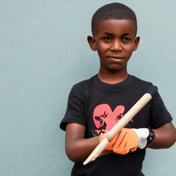
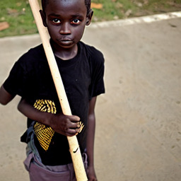
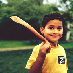
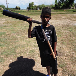
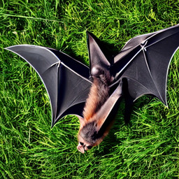
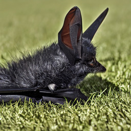
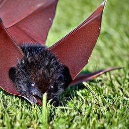
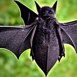
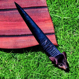
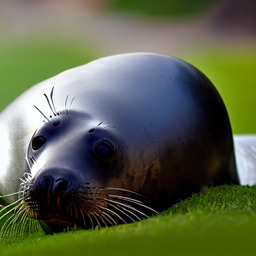
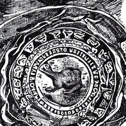
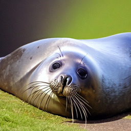
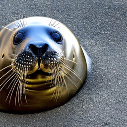
When humans encounter a word with more than one possible meaning, they can use information such as situational context and selectional restrictions to infer which meaning is the most likely. Models for language-based tasks such as translation struggle with this, often being biased towards the sense that is more commonly attested regardless of context and thus often producing a translation of the incorrect sense (Campolungo et al., 2022). Recent research by Rassin et al. (2022) showed that text-to-image diffusion models behave in a different and unexpected way when confronted with a prompt containing polysemous words. Specifically, they showed that when DALL·E 2 is prompted with a sentence containing a word with multiple possible meanings, such as “bat” or “bow”, the generated image often represents more than one of these meanings. For example, in the initial image in Fig. 1bat” is represented both as a baseball bat and an animal. They call this behaviour homonym duplication. Diffusion models have attracted much attention, even beyond the reaches of the research communities that spawned them.111For example, the Twitter account https://twitter.com/weirddalle, which posts images generated by diffusion models, has over 1 million followers at time of writing. Despite this, we are still lacking in our understanding of some of the unusual tendencies they exhibit, such as the phenomenon of homonym duplication.
Refer to caption
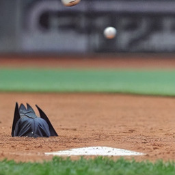
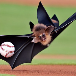
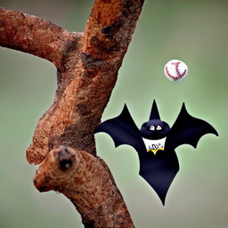
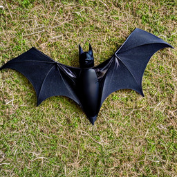
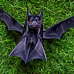
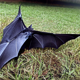
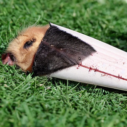
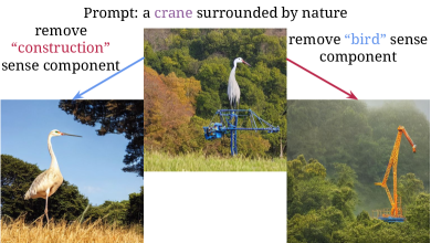
Figure 1: By editing prompt encodings by removing projections of vectors corresponding to each sense, we are able to reduce homonym duplication and produce the desired sense of the word “bat”.

In this work, we put forward one possible explanation of this phenomenon. We suggest that this occurs due to polysemous words in the prompt being encoded as a linear superposition of their possible meanings. In a text-based decoding task, such as translation, a representation of this form would not pose a problem, as the decoding model ultimately converts its representations into a probability distribution over tokens which it uses to select an output word. Thus, although both possibilities will influence the distribution obtained, it is forced to select a word representing one meaning or the other. However, diffusion models use the representation as input to condition the denoising process which predicts noise to remove, and such a choice between meanings is never forced. This means that both meanings influence the denoising process, and both meanings can be represented in the final image. To draw an analogy with quantum mechanics, in a famous thought experiment, Schrödinger (1935) described a scenario in which a cat in a box with a radioactive material is poisoned once a particle decay occurs, and suggested that since a particle’s state exists in a superposition of decayed and undecayed states until an observation is made, that the cat must be considered to be both alive and dead until the box is opened. In the translation scenario, the meaning of a word such as “bat” exists as a superposition of possibilities until an “observation” is made by sampling an output word. Since this never happens in diffusion models, the metaphorical box is never opened and the bat continues to be both a baseball bat and an animal.

Unfortunately, the internal workings of DALL·E 2 are not openly accessible, so we test this hypothesis by performing experiments using the implementation of Stable Diffusion (Rombach et al., 2022) available on HuggingFace (Wolf et al., 2020). This is a smaller diffusion model which encodes prompts using a CLIP (Radford et al., 2021) encoder, the same type of encoder used by DALL·E 2. We begin by showing that diffusion models can represent multiple concepts that are in linear superposition, by demonstrating that when Stable Diffusion takes as input a sum of CLIP encodings for two words, both objects can be represented in the generated image (§ 3). We then demonstrate that CLIP encodes polysemous words as a sum over their possible meanings, and that linear-algebraic manipulation of these representations can be used to generate one sense over another (§ 4), as demonstrated in Fig. 1. Combined, these two facts offer a possible explanation for the homonym duplication described by Rassin et al. (2022).

2 Background: Diffusion Models

Text-to-image diffusion models such as DALL·E 2 (Ramesh et al., 2022) and Stable Diffusion (Rombach et al., 2022) take a text prompt as input and generate an image corresponding to the prompt. During training, an image 𝐱0subscript𝐱0\mathbf{x}_{0} is transformed into random noise through the progressive addition of noise sampled from a Gaussian distribution whose mean depends on the image’s current value, i.e. 𝐱t=𝐱t1+ϵtsubscript𝐱𝑡subscript𝐱𝑡1subscriptbold-italic-ϵ𝑡\mathbf{x}_{t}=\mathbf{x}_{t-1}+\boldsymbol{\epsilon}_{t}, ϵt𝒩(αt𝐱t1,(1αt)𝐈)similar-tosubscriptbold-italic-ϵ𝑡𝒩subscript𝛼𝑡subscript𝐱𝑡11subscript𝛼𝑡𝐈\boldsymbol{\epsilon}_{t}\sim\mathcal{N}(\sqrt{\alpha_{t}}\mathbf{x}_{t-1},(1-\alpha_{t})\mathbf{I}) where αtsubscript𝛼𝑡\alpha_{t} is a value controlling the magnitude of the noise added at each step. The model is then trained to gradually denoise these images, step by step, conditioned on a descriptive caption of the image. Once trained, the model will apply this process to random noise to produce an image consistent with a given prompt.

2.1 CLIP Encoding

Both DALL·E 2 and Stable Diffusion encode text prompts using CLIP (Radford et al., 2021). CLIP is trained by jointly training a transformer-based text encoder and a transformer-based image encoder on pairs of images and captions with a contrastive objective – given N𝑁N pairs, it is trained to maximise the cosine similarity between the text and image encodings for these N𝑁N pairs, but also to minimise cosine similarity between the N2Nsuperscript𝑁2𝑁N^{2}-N other pairings.

2.2 Conditioned Denoising Process

Given a prompt 𝐬𝐬\mathbf{s}, diffusion models sample 𝐱T𝒩(𝟎,𝐈)similar-tosubscript𝐱𝑇𝒩0𝐈\mathbf{x}_{T}\sim\mathcal{N}(\mathbf{0},\mathbf{I}) as their initial image. This image is progressively denoised by taking 𝐱t1=𝐱tAtϵ^θ(𝐱t,t𝐬)+Btsubscript𝐱𝑡1subscript𝐱𝑡subscript𝐴𝑡subscript^bold-italic-ϵ𝜃subscript𝐱𝑡conditional𝑡𝐬subscript𝐵𝑡\mathbf{x}_{t-1}=\mathbf{x}_{t}-A_{t}\widehat{\boldsymbol{\epsilon}}_{\theta}(\mathbf{x}_{t},t\mid\mathbf{s})+B_{t}, where Atsubscript𝐴𝑡A_{t} and Btsubscript𝐵𝑡B_{t} are coefficients calculated by a scheduler. To allow generation to be guided by the prompt, ϵ^θ(𝐱t,t𝐬)=ϵθ(𝐱t,t)+γ(ϵθ(𝐱t,t𝐬)ϵθ(𝐱t,t))subscript^bold-italic-ϵ𝜃subscript𝐱𝑡conditional𝑡𝐬subscriptbold-italic-ϵ𝜃subscript𝐱𝑡conditional𝑡𝛾subscriptbold-italic-ϵ𝜃subscript𝐱𝑡conditional𝑡𝐬subscriptbold-italic-ϵ𝜃subscript𝐱𝑡conditional𝑡\widehat{\boldsymbol{\epsilon}}_{\theta}(\mathbf{x}_{t},t\mid\mathbf{s})=\boldsymbol{\epsilon}_{\theta}(\mathbf{x}_{t},t\mid\emptyset)+\gamma\cdot(\boldsymbol{\epsilon}_{\theta}(\mathbf{x}_{t},t\mid\mathbf{s})-\boldsymbol{\epsilon}_{\theta}(\mathbf{x}_{t},t\mid\emptyset)), where γ1𝛾1\gamma\geq 1 describes the strength of guidance and ϵθ(𝐱t,t𝐬)subscriptbold-italic-ϵ𝜃subscript𝐱𝑡conditional𝑡𝐬\boldsymbol{\epsilon}_{\theta}(\mathbf{x}_{t},t\mid\mathbf{s}) is the model that has been trained to predict the noise to remove at each step. ϵθ(𝐱t,t𝐬)subscriptbold-italic-ϵ𝜃subscript𝐱𝑡conditional𝑡𝐬\boldsymbol{\epsilon}_{\theta}(\mathbf{x}_{t},t\mid\mathbf{s}) is generally implemented with a version of U-Net (Ronneberger et al., 2015).

DALL·E 2.

In DALL·E 2, the prompt 𝐬𝐬\mathbf{s} is encoded using CLIP, a CLIP image encoding is predicted using a transformer-based diffusion prior model conditioned on 𝐬𝐬\mathbf{s} and CLIP(𝐬)CLIP𝐬\operatorname{CLIP}(\mathbf{s}). The main diffusion model is then conditioned on this image encoding by projecting it to the appropriate dimension and then concatenating it to the attention context at each layer.

Stable Diffusion.

In Stable Diffusion, the denoising process takes place entirely in the latent space. The starting point 𝐳Tsubscript𝐳𝑇\mathbf{z}_{T} is sampled and then de-noised conditioned on CLIP(𝐬)CLIP𝐬\operatorname{CLIP}(\mathbf{s}). The conditioning is implemented through cross-attention between U-Net representations and a projection of CLIP(𝐬)CLIP𝐬\operatorname{CLIP}(\mathbf{s}). The final output 𝐳0subscript𝐳0\mathbf{z}_{0} is decoded to an image using the decoder of a Variational Auto-encoder (Kingma and Welling, 2014).

2.3 Homonym Duplication in DALL·E 2

Rassin et al. (2022) demonstrate a number of strange behaviours exhibited by DALL·E 2. In this work, we are primarily concerned with the phenomenon of homonym duplication – when multiple senses of a polysemous word are realised in one image. They use a number of prompts to show that when a prompt contains a polysemous word such as “bat” or “bow”, rather than realising the sense that the model deems to be most likely, it often realises both senses in the final image. They also point out that this is observed less frequently in smaller models such as DALL·E Mini and Stable Diffusion.

2.3.1 Stable Diffusion and DALL·E 2

In this work we consider Stable Diffusion in lieu of DALL·E 2. We make this choice since our method directly manipulates the representations used in the generation process, which is not possible in publicly available releases of DALL·E 2. Both are similar in that they both text-to-image generation models based on diffusion and a CLIP encoder. They differ primarily in the fact that Stable Diffusion performs the denoising process entirely in the latent space. DALL·E 2 is also a much larger model in terms of the number of parameters. Our hypothesis, if true, would be more difficult to show in a smaller model with less representational capacity. Because of this, we consider it likely that positive conclusions drawn from this work would also apply to DALL·E 2, though we invite replication of our approach using DALL·E 2.

2.3.2 Homonym Duplication in Stable Diffusion

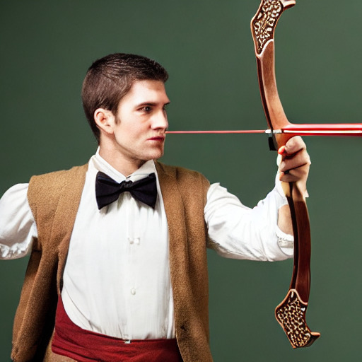
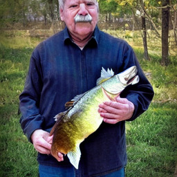
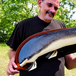
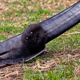
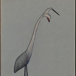
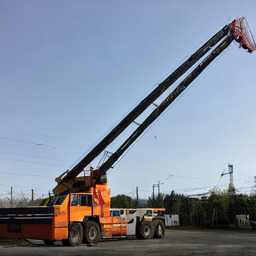
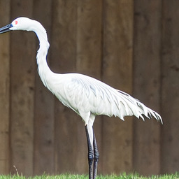
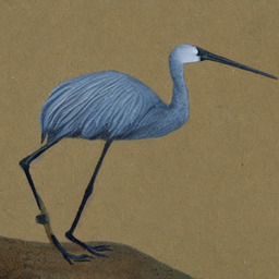
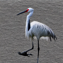
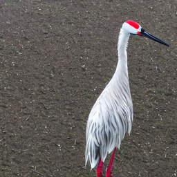
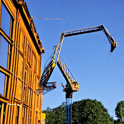
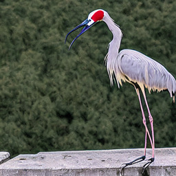
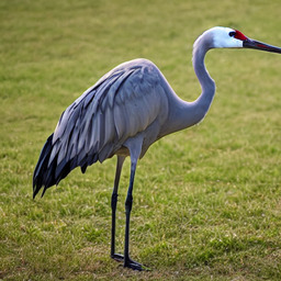
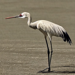
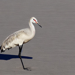
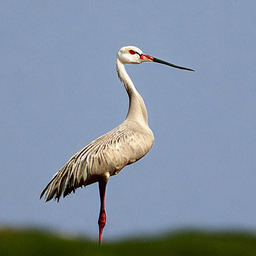
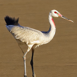
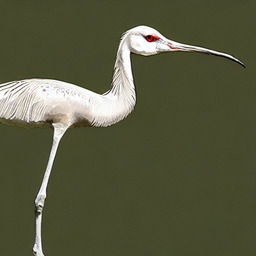
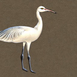
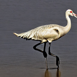
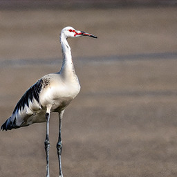
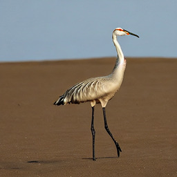
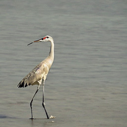
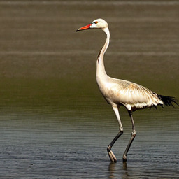
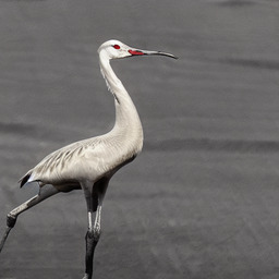
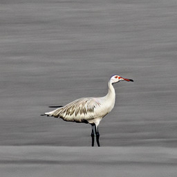
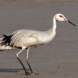
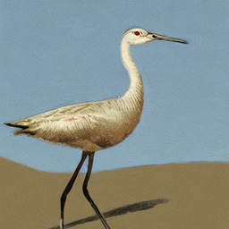
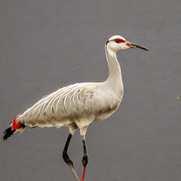
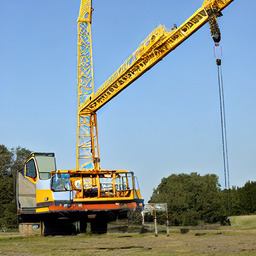
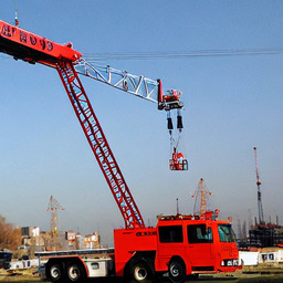
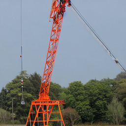
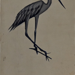
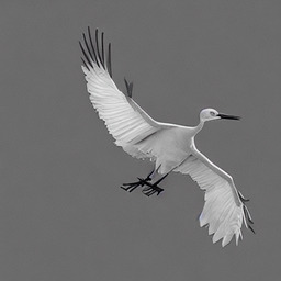
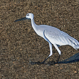
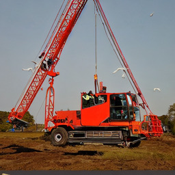
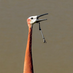
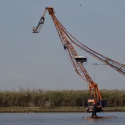
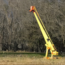
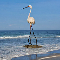
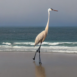
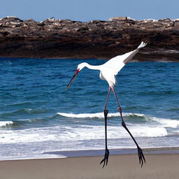
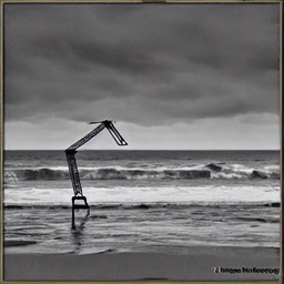
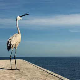
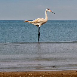
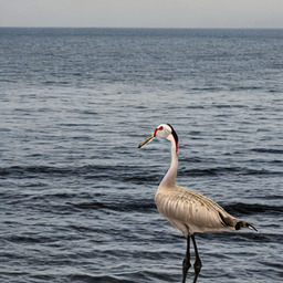
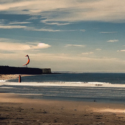
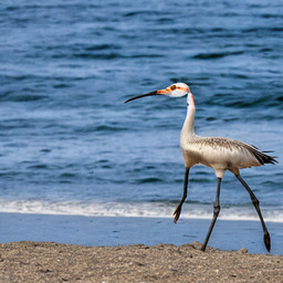
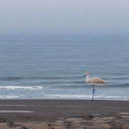
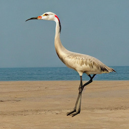
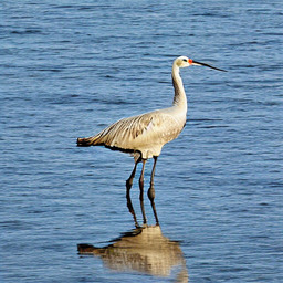
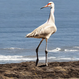
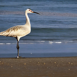
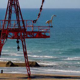
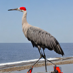
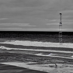
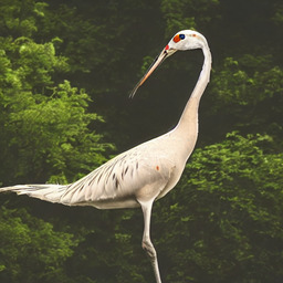
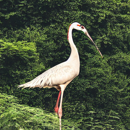
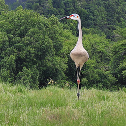
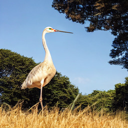
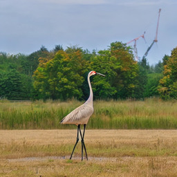
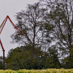
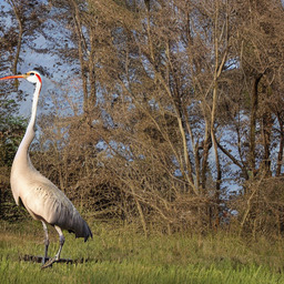
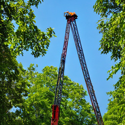
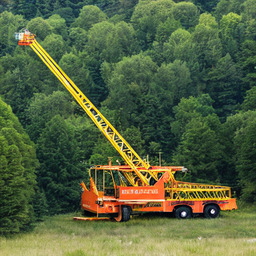
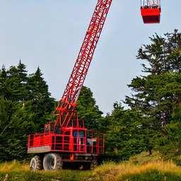
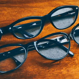
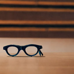
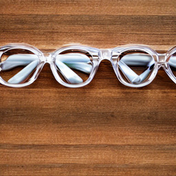
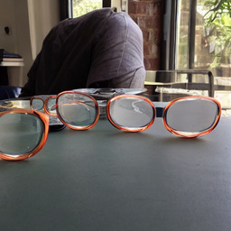
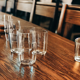
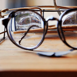
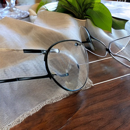
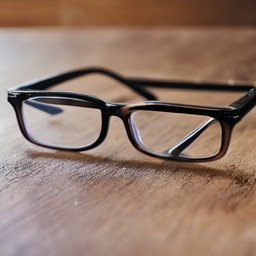
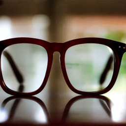
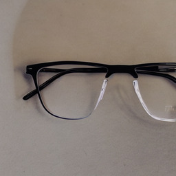
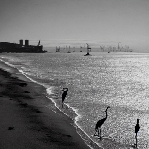
As Rassin et al. (2022) point out, the homonym duplication phenomenon that they observe in DALL·E 2 is seen less frequently in Stable Diffusion. Nonetheless, we were successful in replicating the behaviour for some prompts. Some of these images are shown in Fig. 1 and Fig. 2. More are included in § A.1.
Refer to caption
(a) Prompt: “tall cranes by the sea
Refer to caption
(b) Prompt: “a man holding glasses
Refer to caption
(c) Prompt: “a gentleman with a bow and arrow
Refer to caption
(d) Prompt: “a baseball bat inside a spooky cave
Figure 2: Examples of homonym generation observed in images generated using Stable Diffusion

3 Claim 1: Diffusion can realise multiple concepts in superposition

To construct an explanation for the phenomenon of homonym duplication, we first show that an encoding that is composed of a sum of encodings of multiple words can produce an image in which each word in the sum is represented. When using the model in the standard way, the prompt 𝐬𝐬\mathbf{s} is encoded using CLIP, and the result CLIP(𝐬)CLIP𝐬\operatorname{CLIP}(\mathbf{s}) is then used to condition the denoising process. In these experiments, we instead take two prompts 𝐬1subscript𝐬1\mathbf{s}_{1} and 𝐬2subscript𝐬2\mathbf{s}_{2}, and the denoising process is conditioned on the weighted sum of their CLIP encodings α1CLIP(𝐬1)+α2CLIP(𝐬2)subscript𝛼1CLIPsubscript𝐬1subscript𝛼2CLIPsubscript𝐬2\alpha_{1}\operatorname{CLIP}(\mathbf{s}_{1})+\alpha_{2}\operatorname{CLIP}(\mathbf{s}_{2}), where α1,α2subscript𝛼1subscript𝛼2\alpha_{1},\alpha_{2}\in\mathbb{R} and α1+α2=1subscript𝛼1subscript𝛼21\alpha_{1}+\alpha_{2}=1.222In practice, we achieved best results with α1=α2=0.5subscript𝛼1subscript𝛼20.5\alpha_{1}=\alpha_{2}=0.5.

3.1 Experimental Results

Refer to caption
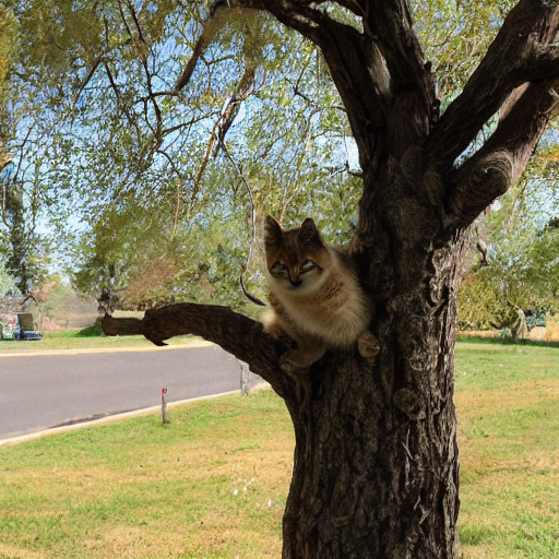
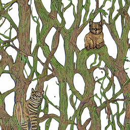
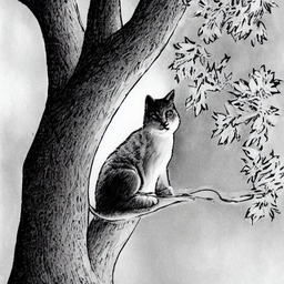
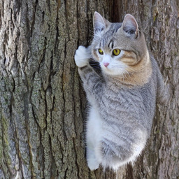
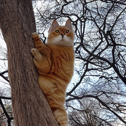
(a) (0.5CLIP(cat))0.5CLIPcat(0.5\cdot\operatorname{CLIP}(\text{``{cat}''})) +(0.5CLIP(tree))0.5CLIPtree+(0.5\cdot\operatorname{CLIP}(\text{``{tree}''}))
Refer to caption
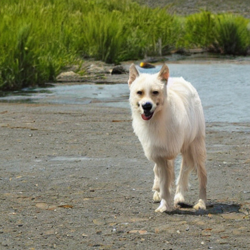
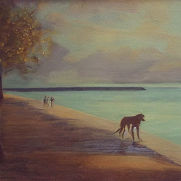
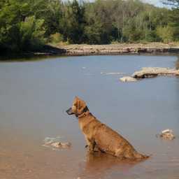
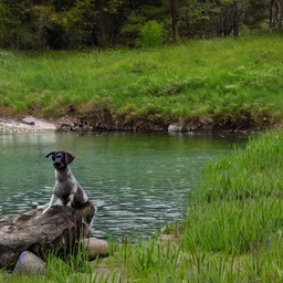
(b) (0.5CLIP(dog))0.5CLIPdog(0.5\cdot\operatorname{CLIP}(\text{``{dog}''})) +(0.5CLIP(lake))0.5CLIPlake+(0.5\cdot\operatorname{CLIP}(\text{``{lake}''}))
Refer to caption
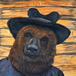
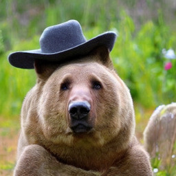
(c) (0.5CLIP(bear))0.5CLIPbear(0.5\cdot\operatorname{CLIP}(\text{``{bear}''})) +(0.5CLIP(hat))0.5CLIPhat+(0.5\cdot\operatorname{CLIP}(\text{``{hat}''}))
Refer to caption
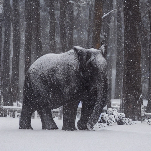
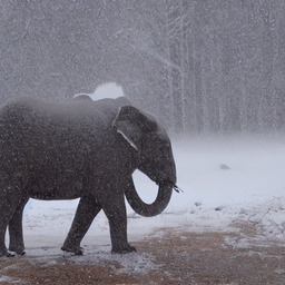
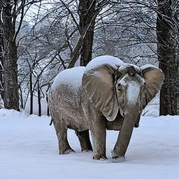
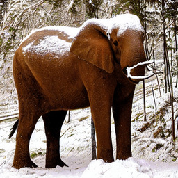
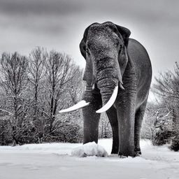
(d) (0.5CLIP(elephant))0.5CLIPelephant(0.5\cdot\operatorname{CLIP}(\text{``{elephant}''})) +(0.5CLIP(snow))0.5CLIPsnow+(0.5\cdot\operatorname{CLIP}(\text{``{snow}''}))
Refer to caption
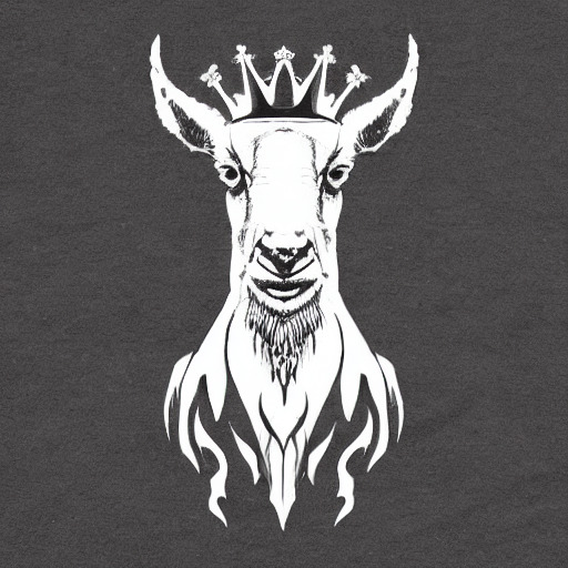
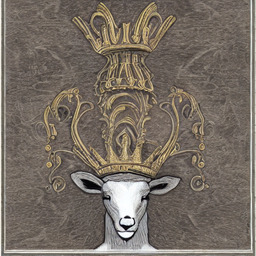
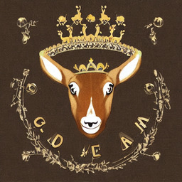
(e) (0.5CLIP(goat))0.5CLIPgoat(0.5\cdot\operatorname{CLIP}(\text{``{goat}''})) +(0.5CLIP(crown))0.5CLIPcrown+(0.5\cdot\operatorname{CLIP}(\text{``{crown}''}))
Refer to caption
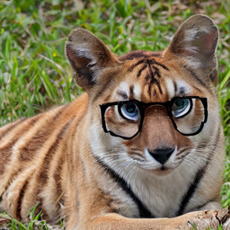
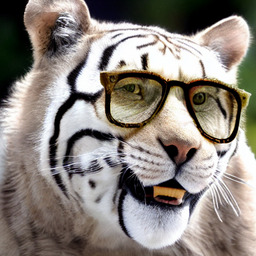
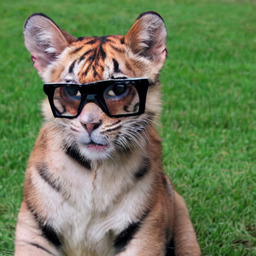
(f) (0.5CLIP(tiger))0.5CLIPtiger(0.5\cdot\operatorname{CLIP}(\text{``{tiger}''})) +(0.5CLIP(glasses))0.5CLIPglasses+(0.5\cdot\operatorname{CLIP}(\text{``{glasses}''}))
Figure 3: Images generated by summing representations of multiple prompts

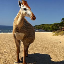
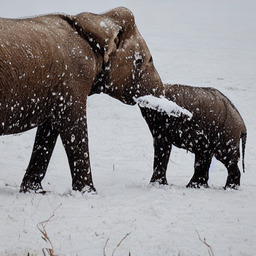
For each pair of prompts, 𝐬1subscript𝐬1\mathbf{s}_{1} and 𝐬2subscript𝐬2\mathbf{s}_{2}, 30 images were generated from α1CLIP(𝐬1)+α2CLIP(𝐬2)subscript𝛼1CLIPsubscript𝐬1subscript𝛼2CLIPsubscript𝐬2\alpha_{1}\operatorname{CLIP}(\mathbf{s}_{1})+\alpha_{2}\operatorname{CLIP}(\mathbf{s}_{2}), 30 images were generated from CLIP(𝐬1)CLIPsubscript𝐬1\operatorname{CLIP}(\mathbf{s}_{1}) and 30 images were generated from CLIP(𝐬2)CLIPsubscript𝐬2\operatorname{CLIP}(\mathbf{s}_{2}). Results presented here are for pairs that were observed to result in realisation of both prompts. Some of the images generated using this method are shown in Fig. 3, and table 1 shows the percentage of images generated that contained the object described by 𝐬1subscript𝐬1\mathbf{s}_{1}, that described by 𝐬2subscript𝐬2\mathbf{s}_{2}, both or neither. We can see that the model can, in fact, generate an image representing both of the words in the sum. In fact, we see that this occurs in over 40% of generated images. More generated images are included in § A.2.1 and a detailed breakdown of the contents of the images generated for each pair of prompts, along with details of statistical significance tests are given in § B.1.

There is no particular reason to assume that summing the representations of two words would result in a representation that can be interpreted by the model. Adding the representations in this way could result in a representation that doesn’t correspond to anything at all, and leads to the generation of low quality images. It’s also plausible that it would produce an interpolation between the two concepts described. However, we can see that this is not the case. The model sometimes produced both of the objects described in the two prompts, and otherwise largely produced one or the other. This indicates that the representations are encoded in such a way that the important information corresponding to each prompt does not interfere when the two are summed, potentially because they are stored in directions that are close to orthogonal.

As an additional observation on this point, we found that some pairs, such as 𝐬1=subscript𝐬1absent\mathbf{s}_{1}=cat”, 𝐬2=subscript𝐬2absent\mathbf{s}_{2}=dog”, did not behave in the same way, instead producing a cat-dog hybrid creature. We speculate that this may be because similar concepts such as “cat” and “dog” are likely to share similar representation space.

Percentage containing:
Input 𝐬1subscript𝐬1\mathbf{s}_{1} 𝐬2subscript𝐬2\mathbf{s}_{2} Both Neither
CLIP(𝐬1)CLIPsubscript𝐬1\operatorname{CLIP}(\mathbf{s}_{1}) 100.0 0 0 0
CLIP(𝐬2)CLIPsubscript𝐬2\operatorname{CLIP}(\mathbf{s}_{2}) 0 100.0 0 0
0.5(CLIP(𝐬1))+limit-from0.5CLIPsubscript𝐬10.5\cdot(\operatorname{CLIP}(\mathbf{s}_{1}))+
0.5(CLIP(𝐬2))0.5CLIPsubscript𝐬20.5\cdot(\operatorname{CLIP}(\mathbf{s}_{2}))
35.2 20 41.5 3.3
Table 1: Table showing which prompts were represented in images generated from each prompt in a pair and from their weighted sum

4 Claim 2: Polysemous words are represented as linear superpositions of meanings

Next, we seek to show that the CLIP encoder used by Stable Diffusion represents polysemous word as a linear superposition of their possible meanings. Other methods of encoding words have been previously shown to represent polysemy in this way (Arora et al., 2018). In this case, since the encoder is transformer-based, there is no static representation of each word, but instead a representation of each token of the word in the context of a sentence. Due to this, we instead approximate directions corresponding to each meaning across several sentences. For a particular word of interest, we take several sets of syntactically similar sentences where each sentence contains either an ambiguous use of the word, or a use where one sense is more likely than the other. A procedure similar to that used by Bolukbasi et al. (2016) is then used to obtain bases for the spaces corresponding to the difference between a representation of a particular meaning and the representation of the word in the corresponding ambiguous sentence. We then use projections into these spaces to obtain approximations of the representation of each meaning. We then demonstrate how these approximations can be used to intervene on a representation and change the sense that appears in generated images. This involves editing the representation in the subspace spanned by our approximate representations, and removing the contribution from the representation of the undesired meaning.

4.1 Identifying a Meaning Subspace
Refer to caption
Refer to caption
Refer to caption
(a) Unedited prompt encoding
Refer to caption
Refer to caption
Refer to caption
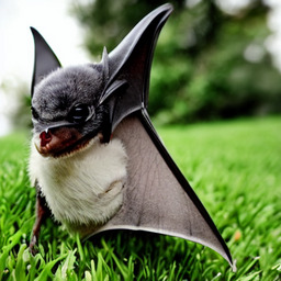
(b) Encoding edited to favour the animal sense
Refer to caption
Refer to caption
Refer to caption
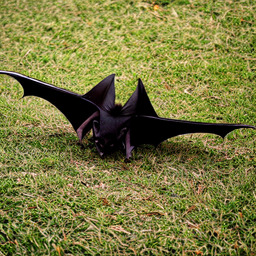
(c) Encoding edited to favour the sports-related sense
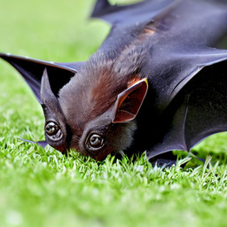
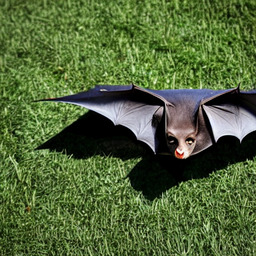
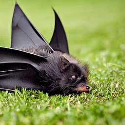
Figure 4: Prompt: “a bat laying on the grass
Refer to caption
Refer to caption
Refer to caption
(a) Unedited prompt encoding
Refer to caption
Refer to caption
Refer to caption
(b) Encoding edited to favour the music-related sense
Refer to caption
Refer to caption
Refer to caption
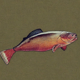
(c) Encoding edited to favour the fish sense
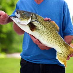
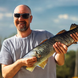
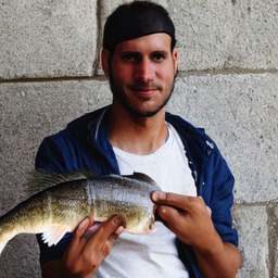
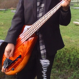
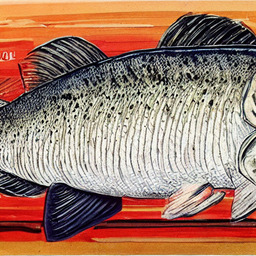
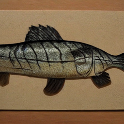
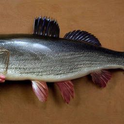
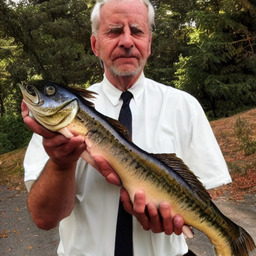
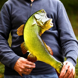
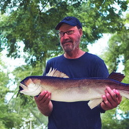
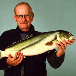
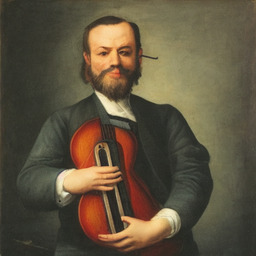
Figure 5: Prompt: “a man holding a bass

In a procedure based on that described by Bolukbasi et al. (2016), we begin by identifying a subspace in which representations of different meanings differ. Given a polysemous word wpsubscript𝑤𝑝w_{p} with distinct possible meanings, m1subscript𝑚1{\color[rgb]{0.390625,0.5859375,0.9296875}\definecolor[named]{pgfstrokecolor}{rgb}{0.390625,0.5859375,0.9296875}m_{1}} and m2subscript𝑚2{\color[rgb]{0.73046875,0.15234375,0.2890625}\definecolor[named]{pgfstrokecolor}{rgb}{0.73046875,0.15234375,0.2890625}m_{2}}, we hand-write a set of N𝑁N prompts containing wpsubscript𝑤𝑝w_{p} in which either of the two candidate meanings is possible. From each such prompt, 𝐬ambsuperscript𝐬amb\mathbf{s}^{{\color[rgb]{0.5625,0.3671875,0.61328125}\definecolor[named]{pgfstrokecolor}{rgb}{0.5625,0.3671875,0.61328125}\text{amb}}}, we manually create 𝐬(1)superscript𝐬1\mathbf{s}^{{\color[rgb]{0.390625,0.5859375,0.9296875}\definecolor[named]{pgfstrokecolor}{rgb}{0.390625,0.5859375,0.9296875}(1)}} and 𝐬(2)superscript𝐬2\mathbf{s}^{{\color[rgb]{0.73046875,0.15234375,0.2890625}\definecolor[named]{pgfstrokecolor}{rgb}{0.73046875,0.15234375,0.2890625}(2)}}, which differ from 𝐬ambsuperscript𝐬amb\mathbf{s}^{{\color[rgb]{0.5625,0.3671875,0.61328125}\definecolor[named]{pgfstrokecolor}{rgb}{0.5625,0.3671875,0.61328125}\text{amb}}} by the addition of a disambiguating modifier and changes to the lexical content to more strongly imply meanings m1subscript𝑚1{\color[rgb]{0.390625,0.5859375,0.9296875}\definecolor[named]{pgfstrokecolor}{rgb}{0.390625,0.5859375,0.9296875}m_{1}} and m2subscript𝑚2{\color[rgb]{0.73046875,0.15234375,0.2890625}\definecolor[named]{pgfstrokecolor}{rgb}{0.73046875,0.15234375,0.2890625}m_{2}} respectively, but otherwise have the same syntactic structure. For example,

𝐬ambsuperscript𝐬amb\displaystyle\mathbf{s}^{{\color[rgb]{0.5625,0.3671875,0.61328125}\definecolor[named]{pgfstrokecolor}{rgb}{0.5625,0.3671875,0.61328125}\text{amb}}} = bat in a boxabsent bat in a box\displaystyle=\text{``{a {\color[rgb]{0.5625,0.3671875,0.61328125}\definecolor[named]{pgfstrokecolor}{rgb}{0.5625,0.3671875,0.61328125} bat} in a box}''}
𝐬(1)superscript𝐬1\displaystyle\mathbf{s}^{{\color[rgb]{0.390625,0.5859375,0.9296875}\definecolor[named]{pgfstrokecolor}{rgb}{0.390625,0.5859375,0.9296875}(1)}} =a vampire  bat in a caveabsenta vampire  bat in a cave\displaystyle=\text{``{a vampire {\color[rgb]{0.390625,0.5859375,0.9296875}\definecolor[named]{pgfstrokecolor}{rgb}{0.390625,0.5859375,0.9296875} bat} in a cave}''}
𝐬(2)superscript𝐬2\displaystyle\mathbf{s}^{{\color[rgb]{0.73046875,0.15234375,0.2890625}\definecolor[named]{pgfstrokecolor}{rgb}{0.73046875,0.15234375,0.2890625}(2)}} =a baseball  bat in a lockerabsenta baseball  bat in a locker\displaystyle=\text{``{a baseball {\color[rgb]{0.73046875,0.15234375,0.2890625}\definecolor[named]{pgfstrokecolor}{rgb}{0.73046875,0.15234375,0.2890625} bat} in a locker}''}

Each sentence is encoded using CLIP and the vector representing wpsubscript𝑤𝑝w_{p} is extracted from each to give Vwp𝐬n={𝐯wp𝐬namb,𝐯wp𝐬n(1),𝐯wp𝐬n(2)}superscriptsubscript𝑉subscript𝑤𝑝subscript𝐬𝑛superscriptsubscript𝐯subscript𝑤𝑝superscriptsubscript𝐬𝑛ambsuperscriptsubscript𝐯subscript𝑤𝑝superscriptsubscript𝐬𝑛1superscriptsubscript𝐯subscript𝑤𝑝superscriptsubscript𝐬𝑛2V_{w_{p}}^{\mathbf{s}_{n}}=\Big{\{}\mathbf{v}_{w_{p}}^{\mathbf{s}_{n}^{{\color[rgb]{0.5625,0.3671875,0.61328125}\definecolor[named]{pgfstrokecolor}{rgb}{0.5625,0.3671875,0.61328125}\text{amb}}}},\mathbf{v}_{w_{p}}^{\mathbf{s}_{n}^{{\color[rgb]{0.390625,0.5859375,0.9296875}\definecolor[named]{pgfstrokecolor}{rgb}{0.390625,0.5859375,0.9296875}(1)}}},\mathbf{v}_{w_{p}}^{\mathbf{s}_{n}^{{\color[rgb]{0.73046875,0.15234375,0.2890625}\definecolor[named]{pgfstrokecolor}{rgb}{0.73046875,0.15234375,0.2890625}(2)}}}\Big{\}}, where 𝐯wp𝐬=CLIP(𝐬)wp\mathbf{v}_{w_{p}}^{\mathbf{s}}=\operatorname{CLIP}(\mathbf{s})_{w_{p}}.333In practice, all of the words we used in our experiments were tokenised to a single token, so our description assumes that we have one encoding per word. For a word consisting of multiple tokens, this process would be repeated for the encoding corresponding to each token.

Next we construct Dnamb1={𝐯wp𝐬namb,𝐯wp𝐬n(1)}subscriptsuperscript𝐷amb1𝑛superscriptsubscript𝐯subscript𝑤𝑝superscriptsubscript𝐬𝑛ambsuperscriptsubscript𝐯subscript𝑤𝑝superscriptsubscript𝐬𝑛1D^{{\color[rgb]{0.5625,0.3671875,0.61328125}\definecolor[named]{pgfstrokecolor}{rgb}{0.5625,0.3671875,0.61328125}\text{amb}}\rightarrow{\color[rgb]{0.390625,0.5859375,0.9296875}\definecolor[named]{pgfstrokecolor}{rgb}{0.390625,0.5859375,0.9296875}1}}_{n}=\Big{\{}\mathbf{v}_{w_{p}}^{\mathbf{s}_{n}^{{\color[rgb]{0.5625,0.3671875,0.61328125}\definecolor[named]{pgfstrokecolor}{rgb}{0.5625,0.3671875,0.61328125}\text{amb}}}},\mathbf{v}_{w_{p}}^{\mathbf{s}_{n}^{{\color[rgb]{0.390625,0.5859375,0.9296875}\definecolor[named]{pgfstrokecolor}{rgb}{0.390625,0.5859375,0.9296875}(1)}}}\Big{\}}, and calculate the mean of each such set:

𝝁namb1=1|Dnamb1|𝐯Dnamb1𝐯subscriptsuperscript𝝁amb1𝑛1subscriptsuperscript𝐷amb1𝑛subscript𝐯subscriptsuperscript𝐷amb1𝑛𝐯\boldsymbol{\mu}^{{\color[rgb]{0.5625,0.3671875,0.61328125}\definecolor[named]{pgfstrokecolor}{rgb}{0.5625,0.3671875,0.61328125}\text{amb}}\rightarrow{\color[rgb]{0.390625,0.5859375,0.9296875}\definecolor[named]{pgfstrokecolor}{rgb}{0.390625,0.5859375,0.9296875}1}}_{n}=\frac{1}{|D^{{\color[rgb]{0.5625,0.3671875,0.61328125}\definecolor[named]{pgfstrokecolor}{rgb}{0.5625,0.3671875,0.61328125}\text{amb}}\rightarrow{\color[rgb]{0.390625,0.5859375,0.9296875}\definecolor[named]{pgfstrokecolor}{rgb}{0.390625,0.5859375,0.9296875}1}}_{n}|}\sum_{\mathbf{v}\in D^{{\color[rgb]{0.5625,0.3671875,0.61328125}\definecolor[named]{pgfstrokecolor}{rgb}{0.5625,0.3671875,0.61328125}\text{amb}}\rightarrow{\color[rgb]{0.390625,0.5859375,0.9296875}\definecolor[named]{pgfstrokecolor}{rgb}{0.390625,0.5859375,0.9296875}1}}_{n}}\mathbf{v} (1)

A matrix is calculated by summing the outer products of each vector’s difference with the mean of its set:

C𝐶\displaystyle C =amb1{}^{{\color[rgb]{0.5625,0.3671875,0.61328125}\definecolor[named]{pgfstrokecolor}{rgb}{0.5625,0.3671875,0.61328125}\text{amb}}\rightarrow{\color[rgb]{0.390625,0.5859375,0.9296875}\definecolor[named]{pgfstrokecolor}{rgb}{0.390625,0.5859375,0.9296875}1}}= (2)
n=1N𝐯Dnamb1(𝐯𝝁namb1)(𝐯𝝁namb1)superscriptsubscript𝑛1𝑁subscript𝐯subscriptsuperscript𝐷amb1𝑛𝐯subscriptsuperscript𝝁amb1𝑛superscript𝐯subscriptsuperscript𝝁amb1𝑛top\displaystyle\sum_{n=1}^{N}\sum_{\mathbf{v}\in D^{{\color[rgb]{0.5625,0.3671875,0.61328125}\definecolor[named]{pgfstrokecolor}{rgb}{0.5625,0.3671875,0.61328125}\text{amb}}\rightarrow{\color[rgb]{0.390625,0.5859375,0.9296875}\definecolor[named]{pgfstrokecolor}{rgb}{0.390625,0.5859375,0.9296875}1}}_{n}}(\mathbf{v}-\boldsymbol{\mu}^{{\color[rgb]{0.5625,0.3671875,0.61328125}\definecolor[named]{pgfstrokecolor}{rgb}{0.5625,0.3671875,0.61328125}\text{amb}}\rightarrow{\color[rgb]{0.390625,0.5859375,0.9296875}\definecolor[named]{pgfstrokecolor}{rgb}{0.390625,0.5859375,0.9296875}1}}_{n})(\mathbf{v}-\boldsymbol{\mu}^{{\color[rgb]{0.5625,0.3671875,0.61328125}\definecolor[named]{pgfstrokecolor}{rgb}{0.5625,0.3671875,0.61328125}\text{amb}}\rightarrow{\color[rgb]{0.390625,0.5859375,0.9296875}\definecolor[named]{pgfstrokecolor}{rgb}{0.390625,0.5859375,0.9296875}1}}_{n})^{\top}

The singular value decomposition (SVD) gives Camb1=U1Σ1V1superscript𝐶amb1subscript𝑈1subscriptΣ1superscriptsubscript𝑉1topC^{{\color[rgb]{0.5625,0.3671875,0.61328125}\definecolor[named]{pgfstrokecolor}{rgb}{0.5625,0.3671875,0.61328125}\text{amb}}\rightarrow{\color[rgb]{0.390625,0.5859375,0.9296875}\definecolor[named]{pgfstrokecolor}{rgb}{0.390625,0.5859375,0.9296875}1}}=U_{{\color[rgb]{0.390625,0.5859375,0.9296875}\definecolor[named]{pgfstrokecolor}{rgb}{0.390625,0.5859375,0.9296875}1}}\Sigma_{{\color[rgb]{0.390625,0.5859375,0.9296875}\definecolor[named]{pgfstrokecolor}{rgb}{0.390625,0.5859375,0.9296875}1}}V_{{\color[rgb]{0.390625,0.5859375,0.9296875}\definecolor[named]{pgfstrokecolor}{rgb}{0.390625,0.5859375,0.9296875}1}}^{\top}. The first k𝑘k columns of the matrix U1subscript𝑈1U_{{\color[rgb]{0.390625,0.5859375,0.9296875}\definecolor[named]{pgfstrokecolor}{rgb}{0.390625,0.5859375,0.9296875}1}}, {𝐮1amb1,,𝐮kamb1}subscriptsuperscript𝐮amb11subscriptsuperscript𝐮amb1𝑘\{\mathbf{u}^{{\color[rgb]{0.5625,0.3671875,0.61328125}\definecolor[named]{pgfstrokecolor}{rgb}{0.5625,0.3671875,0.61328125}\text{amb}}\rightarrow{\color[rgb]{0.390625,0.5859375,0.9296875}\definecolor[named]{pgfstrokecolor}{rgb}{0.390625,0.5859375,0.9296875}1}}_{1},\dots,\mathbf{u}^{{\color[rgb]{0.5625,0.3671875,0.61328125}\definecolor[named]{pgfstrokecolor}{rgb}{0.5625,0.3671875,0.61328125}\text{amb}}\rightarrow{\color[rgb]{0.390625,0.5859375,0.9296875}\definecolor[named]{pgfstrokecolor}{rgb}{0.390625,0.5859375,0.9296875}1}}_{k}\} give an orthonormal basis for the subspace of difference between 𝐯wp𝐬ambsuperscriptsubscript𝐯subscript𝑤𝑝superscript𝐬amb\mathbf{v}_{w_{p}}^{\mathbf{s}^{{\color[rgb]{0.5625,0.3671875,0.61328125}\definecolor[named]{pgfstrokecolor}{rgb}{0.5625,0.3671875,0.61328125}\text{amb}}}} and 𝐯wp𝐬𝐬(1)superscriptsubscript𝐯subscript𝑤𝑝superscript𝐬superscript𝐬1\mathbf{v}_{w_{p}}^{\mathbf{s}^{\mathbf{s}^{{\color[rgb]{0.390625,0.5859375,0.9296875}\definecolor[named]{pgfstrokecolor}{rgb}{0.390625,0.5859375,0.9296875}(1)}}}}.444We choose k𝑘k based on a threshold on the corresponding singular values, specifically we take k𝑘k to be the smallest integer greater than 2 such that i=1kσii=1Nσi>0.95superscriptsubscript𝑖1𝑘subscript𝜎𝑖superscriptsubscript𝑖1𝑁subscript𝜎𝑖0.95\frac{\sum_{i=1}^{k}\sigma_{i}}{\sum_{i=1}^{N}\sigma_{i}}>0.95, where σisubscript𝜎𝑖\sigma_{i} is the i𝑖ith diagonal entry of Σ1subscriptΣ1\Sigma_{{\color[rgb]{0.390625,0.5859375,0.9296875}\definecolor[named]{pgfstrokecolor}{rgb}{0.390625,0.5859375,0.9296875}1}}. In practice, for all of our examples this results in k<5𝑘5k<5. To find {𝐮1amb2,,𝐮kamb2}subscriptsuperscript𝐮amb21subscriptsuperscript𝐮amb2𝑘\{\mathbf{u}^{{\color[rgb]{0.5625,0.3671875,0.61328125}\definecolor[named]{pgfstrokecolor}{rgb}{0.5625,0.3671875,0.61328125}\text{amb}}\rightarrow{\color[rgb]{0.73046875,0.15234375,0.2890625}\definecolor[named]{pgfstrokecolor}{rgb}{0.73046875,0.15234375,0.2890625}2}}_{1},\dots,\mathbf{u}^{{\color[rgb]{0.5625,0.3671875,0.61328125}\definecolor[named]{pgfstrokecolor}{rgb}{0.5625,0.3671875,0.61328125}\text{amb}}\rightarrow{\color[rgb]{0.73046875,0.15234375,0.2890625}\definecolor[named]{pgfstrokecolor}{rgb}{0.73046875,0.15234375,0.2890625}2}}_{k}\}, this procedure is repeated starting with Dnamb2={𝐯wp𝐬namb,𝐯wp𝐬n(2)}subscriptsuperscript𝐷amb2𝑛superscriptsubscript𝐯subscript𝑤𝑝superscriptsubscript𝐬𝑛ambsuperscriptsubscript𝐯subscript𝑤𝑝superscriptsubscript𝐬𝑛2D^{{\color[rgb]{0.5625,0.3671875,0.61328125}\definecolor[named]{pgfstrokecolor}{rgb}{0.5625,0.3671875,0.61328125}\text{amb}}\rightarrow{\color[rgb]{0.73046875,0.15234375,0.2890625}\definecolor[named]{pgfstrokecolor}{rgb}{0.73046875,0.15234375,0.2890625}2}}_{n}=\Big{\{}\mathbf{v}_{w_{p}}^{\mathbf{s}_{n}^{{\color[rgb]{0.5625,0.3671875,0.61328125}\definecolor[named]{pgfstrokecolor}{rgb}{0.5625,0.3671875,0.61328125}\text{amb}}}},\mathbf{v}_{w_{p}}^{\mathbf{s}_{n}^{{\color[rgb]{0.73046875,0.15234375,0.2890625}\definecolor[named]{pgfstrokecolor}{rgb}{0.73046875,0.15234375,0.2890625}(2)}}}\Big{\}}.

4.2 Finding Meaning Directions

We then use the difference subspaces defined by these bases to approximate vectors corresponding to m1subscript𝑚1{\color[rgb]{0.390625,0.5859375,0.9296875}\definecolor[named]{pgfstrokecolor}{rgb}{0.390625,0.5859375,0.9296875}m_{1}} and m2subscript𝑚2{\color[rgb]{0.73046875,0.15234375,0.2890625}\definecolor[named]{pgfstrokecolor}{rgb}{0.73046875,0.15234375,0.2890625}m_{2}}, which we term 𝐯1subscript𝐯1\mathbf{v}_{{\color[rgb]{0.390625,0.5859375,0.9296875}\definecolor[named]{pgfstrokecolor}{rgb}{0.390625,0.5859375,0.9296875}1}} and 𝐯2subscript𝐯2\mathbf{v}_{{\color[rgb]{0.73046875,0.15234375,0.2890625}\definecolor[named]{pgfstrokecolor}{rgb}{0.73046875,0.15234375,0.2890625}2}}.

The procedure for approximating these vectors begins by finding the average projection of 𝐯wp𝐬(1)superscriptsubscript𝐯subscript𝑤𝑝superscript𝐬1\mathbf{v}_{w_{p}}^{\mathbf{s}^{{\color[rgb]{0.390625,0.5859375,0.9296875}\definecolor[named]{pgfstrokecolor}{rgb}{0.390625,0.5859375,0.9296875}(1)}}} into the subspace defined by {𝐮1amb1,,𝐮kamb1}subscriptsuperscript𝐮amb11subscriptsuperscript𝐮amb1𝑘\{\mathbf{u}^{{\color[rgb]{0.5625,0.3671875,0.61328125}\definecolor[named]{pgfstrokecolor}{rgb}{0.5625,0.3671875,0.61328125}\text{amb}}\rightarrow{\color[rgb]{0.390625,0.5859375,0.9296875}\definecolor[named]{pgfstrokecolor}{rgb}{0.390625,0.5859375,0.9296875}1}}_{1},\dots,\mathbf{u}^{{\color[rgb]{0.5625,0.3671875,0.61328125}\definecolor[named]{pgfstrokecolor}{rgb}{0.5625,0.3671875,0.61328125}\text{amb}}\rightarrow{\color[rgb]{0.390625,0.5859375,0.9296875}\definecolor[named]{pgfstrokecolor}{rgb}{0.390625,0.5859375,0.9296875}1}}_{k}\}:

𝐯1(0)=j=1k(1Nn=1N𝐯wp𝐬n(1)𝐮jamb1)𝐮jamb1superscriptsubscript𝐯10superscriptsubscript𝑗1𝑘1𝑁superscriptsubscript𝑛1𝑁superscriptsubscript𝐯subscript𝑤𝑝superscriptsubscript𝐬𝑛1subscriptsuperscript𝐮amb1𝑗subscriptsuperscript𝐮amb1𝑗\mathbf{v}_{{\color[rgb]{0.390625,0.5859375,0.9296875}\definecolor[named]{pgfstrokecolor}{rgb}{0.390625,0.5859375,0.9296875}1}}^{(0)}=\sum_{j=1}^{k}\left(\frac{1}{N}\sum_{n=1}^{N}\mathbf{v}_{w_{p}}^{\mathbf{s}_{n}^{{\color[rgb]{0.390625,0.5859375,0.9296875}\definecolor[named]{pgfstrokecolor}{rgb}{0.390625,0.5859375,0.9296875}(1)}}}\cdot\mathbf{u}^{{\color[rgb]{0.5625,0.3671875,0.61328125}\definecolor[named]{pgfstrokecolor}{rgb}{0.5625,0.3671875,0.61328125}\text{amb}}\rightarrow{\color[rgb]{0.390625,0.5859375,0.9296875}\definecolor[named]{pgfstrokecolor}{rgb}{0.390625,0.5859375,0.9296875}1}}_{j}\right)\mathbf{u}^{{\color[rgb]{0.5625,0.3671875,0.61328125}\definecolor[named]{pgfstrokecolor}{rgb}{0.5625,0.3671875,0.61328125}\text{amb}}\rightarrow{\color[rgb]{0.390625,0.5859375,0.9296875}\definecolor[named]{pgfstrokecolor}{rgb}{0.390625,0.5859375,0.9296875}1}}_{j} (3)

We then make this orthogonal to all 𝐯wp𝐬(2)superscriptsubscript𝐯subscript𝑤𝑝superscript𝐬2\mathbf{v}_{w_{p}}^{\mathbf{s}^{{\color[rgb]{0.73046875,0.15234375,0.2890625}\definecolor[named]{pgfstrokecolor}{rgb}{0.73046875,0.15234375,0.2890625}(2)}}}, by taking 𝐯1^^subscript𝐯1\widehat{\mathbf{v}_{{\color[rgb]{0.390625,0.5859375,0.9296875}\definecolor[named]{pgfstrokecolor}{rgb}{0.390625,0.5859375,0.9296875}1}}} to be 𝐯1(N)𝐯1(N)superscriptsubscript𝐯1𝑁normsuperscriptsubscript𝐯1𝑁\frac{\mathbf{v}_{{\color[rgb]{0.390625,0.5859375,0.9296875}\definecolor[named]{pgfstrokecolor}{rgb}{0.390625,0.5859375,0.9296875}1}}^{(N)}}{||\mathbf{v}_{{\color[rgb]{0.390625,0.5859375,0.9296875}\definecolor[named]{pgfstrokecolor}{rgb}{0.390625,0.5859375,0.9296875}1}}^{(N)}||}, where

𝐯1(n)=𝐯1(n1)proj(𝐯1(n1),𝐯wp𝐬n(2))superscriptsubscript𝐯1𝑛superscriptsubscript𝐯1𝑛1projsuperscriptsubscript𝐯1𝑛1superscriptsubscript𝐯subscript𝑤𝑝superscriptsubscript𝐬𝑛2\mathbf{v}_{{\color[rgb]{0.390625,0.5859375,0.9296875}\definecolor[named]{pgfstrokecolor}{rgb}{0.390625,0.5859375,0.9296875}1}}^{(n)}=\mathbf{v}_{{\color[rgb]{0.390625,0.5859375,0.9296875}\definecolor[named]{pgfstrokecolor}{rgb}{0.390625,0.5859375,0.9296875}1}}^{(n-1)}-\operatorname{proj}(\mathbf{v}_{{\color[rgb]{0.390625,0.5859375,0.9296875}\definecolor[named]{pgfstrokecolor}{rgb}{0.390625,0.5859375,0.9296875}1}}^{(n-1)},\mathbf{v}_{w_{p}}^{\mathbf{s}_{n}^{{\color[rgb]{0.73046875,0.15234375,0.2890625}\definecolor[named]{pgfstrokecolor}{rgb}{0.73046875,0.15234375,0.2890625}(2)}}}) (4)

where proj(𝐚,𝐛)proj𝐚𝐛\operatorname{proj}(\mathbf{a},\mathbf{b}) denotes the projection of 𝐚𝐚\mathbf{a} onto 𝐛𝐛\mathbf{b}, i.e. proj(𝐚,𝐛)=𝐚𝐛𝐛𝐛𝐛proj𝐚𝐛𝐚𝐛𝐛𝐛𝐛\operatorname{proj}(\mathbf{a},\mathbf{b})=\frac{\mathbf{a}\cdot\mathbf{b}}{\mathbf{b}\cdot\mathbf{b}}\mathbf{b}. The vector 𝐯2^^subscript𝐯2\widehat{\mathbf{v}_{{\color[rgb]{0.73046875,0.15234375,0.2890625}\definecolor[named]{pgfstrokecolor}{rgb}{0.73046875,0.15234375,0.2890625}2}}} is found analogously.

By examination, we find that representations from ambiguous sentences tend to have negative dot products with both 𝐯1^^subscript𝐯1\widehat{\mathbf{v}_{{\color[rgb]{0.390625,0.5859375,0.9296875}\definecolor[named]{pgfstrokecolor}{rgb}{0.390625,0.5859375,0.9296875}1}}} and 𝐯2^^subscript𝐯2\widehat{\mathbf{v}_{{\color[rgb]{0.73046875,0.15234375,0.2890625}\definecolor[named]{pgfstrokecolor}{rgb}{0.73046875,0.15234375,0.2890625}2}}} (or occasionally positive dot products with both). Representations from sentences favouring m1subscript𝑚1{\color[rgb]{0.390625,0.5859375,0.9296875}\definecolor[named]{pgfstrokecolor}{rgb}{0.390625,0.5859375,0.9296875}m_{1}} tend to have a a positive dot product with 𝐯1^^subscript𝐯1\widehat{\mathbf{v}_{{\color[rgb]{0.390625,0.5859375,0.9296875}\definecolor[named]{pgfstrokecolor}{rgb}{0.390625,0.5859375,0.9296875}1}}} and a near-zero dot product with 𝐯2^^subscript𝐯2\widehat{\mathbf{v}_{{\color[rgb]{0.73046875,0.15234375,0.2890625}\definecolor[named]{pgfstrokecolor}{rgb}{0.73046875,0.15234375,0.2890625}2}}} (by construction), and vice versa for sentences favouring m2subscript𝑚2{\color[rgb]{0.73046875,0.15234375,0.2890625}\definecolor[named]{pgfstrokecolor}{rgb}{0.73046875,0.15234375,0.2890625}m_{2}}. This suggests how we may edit representations to target a desired sense.

The normalised vectors 𝐯1^^subscript𝐯1\widehat{\mathbf{v}_{{\color[rgb]{0.390625,0.5859375,0.9296875}\definecolor[named]{pgfstrokecolor}{rgb}{0.390625,0.5859375,0.9296875}1}}} and 𝐯2^^subscript𝐯2\widehat{\mathbf{v}_{{\color[rgb]{0.73046875,0.15234375,0.2890625}\definecolor[named]{pgfstrokecolor}{rgb}{0.73046875,0.15234375,0.2890625}2}}} are not used, instead we take 𝐯1=maxn(𝐯wp𝐬n(1)𝐯1^)𝐯1^subscript𝐯1subscript𝑛superscriptsubscript𝐯subscript𝑤𝑝superscriptsubscript𝐬𝑛1^subscript𝐯1^subscript𝐯1\mathbf{v}_{{\color[rgb]{0.390625,0.5859375,0.9296875}\definecolor[named]{pgfstrokecolor}{rgb}{0.390625,0.5859375,0.9296875}1}}=\max_{n}(\mathbf{v}_{w_{p}}^{\mathbf{s}_{n}^{{\color[rgb]{0.390625,0.5859375,0.9296875}\definecolor[named]{pgfstrokecolor}{rgb}{0.390625,0.5859375,0.9296875}(1)}}}\cdot\widehat{\mathbf{v}_{{\color[rgb]{0.390625,0.5859375,0.9296875}\definecolor[named]{pgfstrokecolor}{rgb}{0.390625,0.5859375,0.9296875}1}}})\widehat{\mathbf{v}_{{\color[rgb]{0.390625,0.5859375,0.9296875}\definecolor[named]{pgfstrokecolor}{rgb}{0.390625,0.5859375,0.9296875}1}}} and 𝐯2=maxn(𝐯wp𝐬n(2)𝐯2^)𝐯2^subscript𝐯2subscript𝑛superscriptsubscript𝐯subscript𝑤𝑝superscriptsubscript𝐬𝑛2^subscript𝐯2^subscript𝐯2\mathbf{v}_{{\color[rgb]{0.73046875,0.15234375,0.2890625}\definecolor[named]{pgfstrokecolor}{rgb}{0.73046875,0.15234375,0.2890625}2}}=\max_{n}(\mathbf{v}_{w_{p}}^{\mathbf{s}_{n}^{{\color[rgb]{0.73046875,0.15234375,0.2890625}\definecolor[named]{pgfstrokecolor}{rgb}{0.73046875,0.15234375,0.2890625}(2)}}}\cdot\widehat{\mathbf{v}_{{\color[rgb]{0.73046875,0.15234375,0.2890625}\definecolor[named]{pgfstrokecolor}{rgb}{0.73046875,0.15234375,0.2890625}2}}})\widehat{\mathbf{v}_{{\color[rgb]{0.73046875,0.15234375,0.2890625}\definecolor[named]{pgfstrokecolor}{rgb}{0.73046875,0.15234375,0.2890625}2}}}. We do this so that the vector also represents the magnitude of projection is this direction that is sufficient to have this sense represented.

4.3 Sense Editing Procedure

If we have a sentence 𝐬𝐬\mathbf{s} containing wpsubscript𝑤𝑝w_{p} then its standard, unedited encoding is given by 𝐯wp=CLIP(𝐬)wp\mathbf{v}_{w_{p}}=\operatorname{CLIP}(\mathbf{s})_{w_{p}}. To edit this representation to push its sense towards m2subscript𝑚2{\color[rgb]{0.73046875,0.15234375,0.2890625}\definecolor[named]{pgfstrokecolor}{rgb}{0.73046875,0.15234375,0.2890625}m_{2}}, we consider its projection onto the subspace spanned by 𝐯1subscript𝐯1\mathbf{v}_{{\color[rgb]{0.390625,0.5859375,0.9296875}\definecolor[named]{pgfstrokecolor}{rgb}{0.390625,0.5859375,0.9296875}1}} and 𝐯2subscript𝐯2\mathbf{v}_{{\color[rgb]{0.73046875,0.15234375,0.2890625}\definecolor[named]{pgfstrokecolor}{rgb}{0.73046875,0.15234375,0.2890625}2}} and aim to make its dot product with 𝐯1subscript𝐯1\mathbf{v}_{{\color[rgb]{0.390625,0.5859375,0.9296875}\definecolor[named]{pgfstrokecolor}{rgb}{0.390625,0.5859375,0.9296875}1}} in this subspace near-zero while aligning it with 𝐯2subscript𝐯2\mathbf{v}_{{\color[rgb]{0.73046875,0.15234375,0.2890625}\definecolor[named]{pgfstrokecolor}{rgb}{0.73046875,0.15234375,0.2890625}2}}, based on the observations described in the previous section.

Since 𝐯1subscript𝐯1\mathbf{v}_{{\color[rgb]{0.390625,0.5859375,0.9296875}\definecolor[named]{pgfstrokecolor}{rgb}{0.390625,0.5859375,0.9296875}1}} and 𝐯2subscript𝐯2\mathbf{v}_{{\color[rgb]{0.73046875,0.15234375,0.2890625}\definecolor[named]{pgfstrokecolor}{rgb}{0.73046875,0.15234375,0.2890625}2}} are, in general, not orthogonal, we first obtain an orthonormal basis of the subspace that they span: U={𝐯1𝐯1,𝐯2proj(𝐯2,𝐯1𝐯1)𝐯2proj(𝐯2,𝐯1𝐯1)}𝑈subscript𝐯1normsubscript𝐯1subscript𝐯2projsubscript𝐯2subscript𝐯1normsubscript𝐯1normsubscript𝐯2projsubscript𝐯2subscript𝐯1normsubscript𝐯1U=\left\{\frac{\mathbf{v}_{{\color[rgb]{0.390625,0.5859375,0.9296875}\definecolor[named]{pgfstrokecolor}{rgb}{0.390625,0.5859375,0.9296875}1}}}{||\mathbf{v}_{{\color[rgb]{0.390625,0.5859375,0.9296875}\definecolor[named]{pgfstrokecolor}{rgb}{0.390625,0.5859375,0.9296875}1}}||},\frac{\mathbf{v}_{{\color[rgb]{0.73046875,0.15234375,0.2890625}\definecolor[named]{pgfstrokecolor}{rgb}{0.73046875,0.15234375,0.2890625}2}}-\operatorname{proj}(\mathbf{v}_{{\color[rgb]{0.73046875,0.15234375,0.2890625}\definecolor[named]{pgfstrokecolor}{rgb}{0.73046875,0.15234375,0.2890625}2}},\frac{\mathbf{v}_{{\color[rgb]{0.390625,0.5859375,0.9296875}\definecolor[named]{pgfstrokecolor}{rgb}{0.390625,0.5859375,0.9296875}1}}}{||\mathbf{v}_{{\color[rgb]{0.390625,0.5859375,0.9296875}\definecolor[named]{pgfstrokecolor}{rgb}{0.390625,0.5859375,0.9296875}1}}||})}{||\mathbf{v}_{{\color[rgb]{0.73046875,0.15234375,0.2890625}\definecolor[named]{pgfstrokecolor}{rgb}{0.73046875,0.15234375,0.2890625}2}}-\operatorname{proj}(\mathbf{v}_{{\color[rgb]{0.73046875,0.15234375,0.2890625}\definecolor[named]{pgfstrokecolor}{rgb}{0.73046875,0.15234375,0.2890625}2}},\frac{\mathbf{v}_{{\color[rgb]{0.390625,0.5859375,0.9296875}\definecolor[named]{pgfstrokecolor}{rgb}{0.390625,0.5859375,0.9296875}1}}}{||\mathbf{v}_{{\color[rgb]{0.390625,0.5859375,0.9296875}\definecolor[named]{pgfstrokecolor}{rgb}{0.390625,0.5859375,0.9296875}1}}||})||}\right\}, and then compute

𝐯~wpm2=𝐯wpprojU𝐯wpsubscriptsuperscript~𝐯subscript𝑚2subscript𝑤𝑝subscript𝐯subscript𝑤𝑝subscriptproj𝑈subscript𝐯subscript𝑤𝑝\displaystyle\widetilde{\mathbf{v}}^{{\color[rgb]{0.73046875,0.15234375,0.2890625}\definecolor[named]{pgfstrokecolor}{rgb}{0.73046875,0.15234375,0.2890625}m_{2}}}_{w_{p}}=\mathbf{v}_{w_{p}}-\operatorname{proj}_{U}\mathbf{v}_{w_{p}} (5)
+𝐯2𝐯2proj(𝐯2,𝐯1)(𝐯2proj(𝐯2,𝐯1))normsubscript𝐯2normsubscript𝐯2projsubscript𝐯2subscript𝐯1subscript𝐯2projsubscript𝐯2subscript𝐯1\displaystyle+\frac{||\mathbf{v}_{{\color[rgb]{0.73046875,0.15234375,0.2890625}\definecolor[named]{pgfstrokecolor}{rgb}{0.73046875,0.15234375,0.2890625}2}}||}{||\mathbf{v}_{{\color[rgb]{0.73046875,0.15234375,0.2890625}\definecolor[named]{pgfstrokecolor}{rgb}{0.73046875,0.15234375,0.2890625}2}}-\operatorname{proj}(\mathbf{v}_{{\color[rgb]{0.73046875,0.15234375,0.2890625}\definecolor[named]{pgfstrokecolor}{rgb}{0.73046875,0.15234375,0.2890625}2}},\mathbf{v}_{{\color[rgb]{0.390625,0.5859375,0.9296875}\definecolor[named]{pgfstrokecolor}{rgb}{0.390625,0.5859375,0.9296875}1}})||}(\mathbf{v}_{{\color[rgb]{0.73046875,0.15234375,0.2890625}\definecolor[named]{pgfstrokecolor}{rgb}{0.73046875,0.15234375,0.2890625}2}}-\operatorname{proj}(\mathbf{v}_{{\color[rgb]{0.73046875,0.15234375,0.2890625}\definecolor[named]{pgfstrokecolor}{rgb}{0.73046875,0.15234375,0.2890625}2}},\mathbf{v}_{{\color[rgb]{0.390625,0.5859375,0.9296875}\definecolor[named]{pgfstrokecolor}{rgb}{0.390625,0.5859375,0.9296875}1}}))

where projU𝐯subscriptproj𝑈𝐯\operatorname{proj}_{U}\mathbf{v} is the projection onto the subspace defined by U𝑈U, i.e. projU𝐯=𝐮U(𝐯𝐮)𝐮subscriptproj𝑈𝐯subscript𝐮𝑈𝐯𝐮𝐮\operatorname{proj}_{U}\mathbf{v}=\sum_{\mathbf{u}\in U}(\mathbf{v}\cdot\mathbf{u})\mathbf{u}.

Subtracting projU𝐯wpsubscriptproj𝑈subscript𝐯subscript𝑤𝑝\operatorname{proj}_{U}\mathbf{v}_{w_{p}} removes the entire projection of the vector onto this subspace, including its component along 𝐯1subscript𝐯1\mathbf{v}_{{\color[rgb]{0.390625,0.5859375,0.9296875}\definecolor[named]{pgfstrokecolor}{rgb}{0.390625,0.5859375,0.9296875}1}}, making it orthogonal to 𝐯1subscript𝐯1\mathbf{v}_{{\color[rgb]{0.390625,0.5859375,0.9296875}\definecolor[named]{pgfstrokecolor}{rgb}{0.390625,0.5859375,0.9296875}1}} as desired. We then wish to add 𝐯2subscript𝐯2\mathbf{v}_{{\color[rgb]{0.73046875,0.15234375,0.2890625}\definecolor[named]{pgfstrokecolor}{rgb}{0.73046875,0.15234375,0.2890625}2}}, but since this is not orthogonal to 𝐯1subscript𝐯1\mathbf{v}_{{\color[rgb]{0.390625,0.5859375,0.9296875}\definecolor[named]{pgfstrokecolor}{rgb}{0.390625,0.5859375,0.9296875}1}} we remove its projection along 𝐯1subscript𝐯1\mathbf{v}_{{\color[rgb]{0.390625,0.5859375,0.9296875}\definecolor[named]{pgfstrokecolor}{rgb}{0.390625,0.5859375,0.9296875}1}} and rescale accordingly. This means that in the subspace defined by U𝑈U, 𝐯~wpm2subscriptsuperscript~𝐯subscript𝑚2subscript𝑤𝑝\widetilde{\mathbf{v}}^{{\color[rgb]{0.73046875,0.15234375,0.2890625}\definecolor[named]{pgfstrokecolor}{rgb}{0.73046875,0.15234375,0.2890625}m_{2}}}_{w_{p}} is orthogonal to 𝐯1subscript𝐯1\mathbf{v}_{{\color[rgb]{0.390625,0.5859375,0.9296875}\definecolor[named]{pgfstrokecolor}{rgb}{0.390625,0.5859375,0.9296875}1}} and has high cosine similarity with 𝐯2subscript𝐯2\mathbf{v}_{{\color[rgb]{0.73046875,0.15234375,0.2890625}\definecolor[named]{pgfstrokecolor}{rgb}{0.73046875,0.15234375,0.2890625}2}}. This edited representation replaces 𝐯wpsubscript𝐯subscript𝑤𝑝\mathbf{v}_{w_{p}} in the sentence encoding, which is then passed to the model as input.

4.4 Experimental Results

Prompts
a bass a crane
a man holds a bass a crane by the ocean
a bass is displayed on a wall a crane surrounded by nature
a bat glasses on a table
a bat and a baseball fly through the air a seal
a boy holds a black bat a seal on an envelope
a bat laying on the grass a trunk
Table 2: Prompts used to evaluate our editing procedure, with the word of interest in bold
Refer to caption
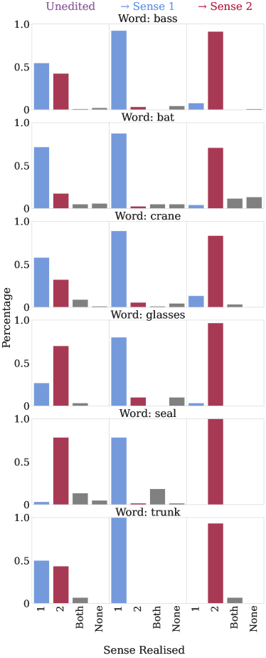
Figure 6: For each word, the proportion of images across all prompts realising each sense is compared across the Unedited encoding, the encoding shifted towards Sense 1 ( \rightarrow Sense 1), and the encoding shifted towards Sense 2 ( \rightarrow Sense 2)

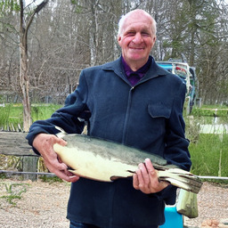
The sense editing procedure was performed on a set of prompts (shown in table 2) that were selected either because they had been observed to exhibit homonym duplication or because the sense that was represented in generated images was not always the same. In Fig. 4 and Fig. 5, we show some example images generated using an unedited prompt and some using prompts edited to favour one sense over another. More images are provided in § A.3. In Fig. 6, we display the proportion of images realising each sense before and after applying this procedure (with \rightarrow Sense 1 and \rightarrow Sense 2 denoting the encodings edited to favour Sense 1 and Sense 2 respectively). Detailed numbers and details of statistical significance testing can be found in § B.2. We can see that this procedure is successful in shifting the represented sense towards the intended sense. This suggests that the representations produced by CLIP do indeed incorporate a linear sum over representations of possible meanings, because a representation can be rewritten in terms of its projection into the subspace spanned by 𝐯1subscript𝐯1\mathbf{v}_{{\color[rgb]{0.390625,0.5859375,0.9296875}\definecolor[named]{pgfstrokecolor}{rgb}{0.390625,0.5859375,0.9296875}1}} and 𝐯2subscript𝐯2\mathbf{v}_{{\color[rgb]{0.73046875,0.15234375,0.2890625}\definecolor[named]{pgfstrokecolor}{rgb}{0.73046875,0.15234375,0.2890625}2}} and a component in the nullspace of this projection. It also shows that manipulating this sum affects the content of the resulting images.

We note that this is, of course, a simplified approach. The directions obtained are an approximation based on a small number of handwritten sentences, and we intervene only on the polysemous word of interest, not on any of the other encodings in the sentence, which may also contain relevant information. Nonetheless, that such a simple and approximate method is capable of achieving such results is a signal in itself.

5 An Explanation for Homonym Duplication

Combining the two claims that we have demonstrated, we arrive at a possible explanation of homonym duplication: words with multiple meanings are represented by a sum over multiple meanings, and both of these are then represented in the generated image. The difficulty inherent to dealing with words with potentially ambiguous meanings is by no means unique to text-to-image diffusion models, and, indeed, previous work has shown that similarly structured representations can arise through other methods Arora et al. (2018). So, it is natural to ask why the phenomenon of duplication has not been observed in text-based models that use such representations. For example, consider a machine translation model translating the phrase “a bat” from English to French. The English word “bat” can correspond to one of multiple words in French,author=ryan,color=violet!40,size=,fancyline,caption=,]I would list them. depending on which sense is intended. Although it is possible that the model’s representation may include contributions from bothauthor=ryan,color=violet!40,size=,fancyline,caption=,]You switched from multiple to both, which implies two. I would just name the two senses in this example. possible meanings, when the decoder comes to generate an output word corresponding to “bat”, this representation will be converted into a distribution over output tokens and only one is sampled, corresponding to one of the two senses. This functionally represents the model selecting that sense over the other. When the next output token is sampled, the model’s output distribution is affected by the previous output and accordingly is very unlikely to generate further tokens corresponding to the other sense as this would produce nonsensical sentences unlike anything seen in training. Such models may produce the incorrect sense in a translation, but they have not been observed to produce both in the way diffusion models do.

In contrast, diffusion models use prompt representations to condition the denoising process. This process produces probability distributions over noise to be removed from the image at each step. This means that, unlike the translation model, the diffusion model is effectively never forced to sample from the possible meanings to select one over the other, and both can be represented in the resultant image. We have seen this to be the case in § 3. This difference is likely why we see this unique behaviour in diffusion models and not in text-based models using similarly-structured representations.

6 Stable Diffusion and DALL·E 2

Rassin et al. (2022) found that smaller models exhibit homonym duplication much less frequently than larger ones. The superposition explanation is consistent with this finding: larger models have a larger representational capacity, and, thus, are capable of representing more features without interference. As shown by Elhage et al. (2022), models with more limited representational capacity may not represent features that do not prove to be sufficiently important. This suggests that smaller models may cease to represent a meaning that is improbable, and, in effect, one meaning is selected, whereas larger models are capable of continuing to represent alternative possible meanings, even if they are modelled to be unlikely.

It is also possible that this difference is a result of the two different processes followed by the models in training and in generating a new image. For a training pair (𝐱,𝐲)𝐱𝐲(\mathbf{x},\mathbf{y}), Stable Diffusion uses a variational autoencoder (Kingma and Welling, 2014) to obtain 𝐳0subscript𝐳0\mathbf{z}_{0}, a representation of 𝐱𝐱\mathbf{x} in latent space. The denoising process is then trained to recover 𝐳0subscript𝐳0\mathbf{z}_{0} from a noised 𝐳Tsubscript𝐳𝑇\mathbf{z}_{T}, conditioned on CLIP(𝐲)CLIP𝐲\operatorname{CLIP}(\mathbf{y}). Since the latent space is learned through autoencoding, it is likely that it will prioritise encoding information necessary to reconstruct the image, and there is no reason why distinct concepts described by a polysemous word should be encoded similarly. Thus, the denoising process of Stable Diffusion may learn to discard this information.

7 Related Work

Previous work has investigated models’ learned representations through the lens of superposition. Elhage et al. (2022) conducted a controlled investigation into superposition in learned representations in feedforward neural networks. They investigated the tendency for a learned feature in a network to correspond to multiple features in superposition, and demonstrated how this allows for efficient storage of important features, allowing a representation to encode more features than it has dimensions. Previous work by Arora et al. (2018) has also found that learned representations of words can represent polysemous words as a linear superposition of possible meanings.

Work modelling inference of the meaning of an ambiguous word also offers some insight. Erk and Herbelot (2021) model this process using a probabilistic graphical model, where meanings are latent variables that are inferred using the information provided by other words, such as the topical context and semantic restrictions. From this perspective, beliefs about the meaning of an ambiguous word are always viewed as a distribution over possible meanings, even if it is skewed so that one is much more likely. If we view computational models as similarly inferring a probability distribution over meanings, text-based decoding models are ultimately forced to sample from the resulting distribution, whereas diffusion models maintain both possibilities throughout the process of generating an image and thus can produce an image containing both.

8 Conclusion

In this work, we set out a possible explanation for the phenomenon of homonym duplication in text-to-image diffusion models as described by Rassin et al. (2022). We showed that summing representations of two distinct prompts and using this as input to the denoising process often leads to images in which both prompts are realised. This suggests that prompts are encoded in such a way that representations of distinct concepts can be summed without substantially interfering with each other. It also demonstrates that the denoising process does not restrict diffusion models to representing only one meaning.

We further described a procedure for manipulating which sense of a polysemous word appears in a generated image, based on the assumption that a representation of such a word contains linear contributions from each possible meaning. We demonstrated this procedure on several prompts, including some that exhibit homonym duplication, finding that it substantially increases the number of generated images containing the targeted sense, even when this sense is only rarely produced using the unedited representation. The success of this manipulation method provides support for the hypothesised structure of the representations.

We suggest that these facts combine to offer a plausible explanation of homonym duplication.

References

Appendix A More Generated Images

In this section we provide a selection of additional images generated during our experiments.

A.1 Homonym Duplication

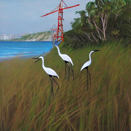
Fig. 7 displays further examples of homonym duplication seen in Stable Diffusion.
Refer to caption
Refer to caption
Refer to caption
Refer to caption
(a) Prompt: “tall cranes by the ocean
Refer to caption
Refer to caption
Refer to caption
Refer to caption
(b) Prompt: “a bat and a baseball fly through the air
Refer to caption
Refer to caption
(c) Prompt: “a woman with a silk bow and arrow
Figure 7: Examples of homonym duplication

A.2 Summing Encodings

Here we include further examples of images generated from the weighted sum of two prompt encodings as described in § 3.

A.2.1 Both Concepts Realised

In Fig. 8 we include examples of images where both concepts in the sum are realised in the final image.
Refer to caption
Refer to caption
Refer to caption
Refer to caption
Refer to caption
Refer to caption
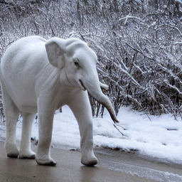
(a) (0.5CLIP(elephant))+(0.5CLIP(snow))0.5CLIPelephant0.5CLIPsnow(0.5\cdot\operatorname{CLIP}(\text{``{elephant}''}))+(0.5\cdot\operatorname{CLIP}(\text{``{snow}''}))
Refer to caption
Refer to caption
Refer to caption
Refer to caption
Refer to caption
Refer to caption
(b) (0.5CLIP(goat))+(0.5CLIP(crown))0.5CLIPgoat0.5CLIPcrown(0.5\cdot\operatorname{CLIP}(\text{``{goat}''}))+(0.5\cdot\operatorname{CLIP}(\text{``{crown}''}))
Refer to caption
Refer to caption
Refer to caption
Refer to caption
Refer to caption
Refer to caption
(c) (0.5CLIP(tiger))+(0.5CLIP(glasses))0.5CLIPtiger0.5CLIPglasses(0.5\cdot\operatorname{CLIP}(\text{``{tiger}''}))+(0.5\cdot\operatorname{CLIP}(\text{``{glasses}''}))
Refer to caption
Refer to caption
Refer to caption
Refer to caption
Refer to caption
Refer to caption
(d) (0.5CLIP(bear))+(0.5CLIP(hat))0.5CLIPbear0.5CLIPhat(0.5\cdot\operatorname{CLIP}(\text{``{bear}''}))+(0.5\cdot\operatorname{CLIP}(\text{``{hat}''}))
Refer to caption
Refer to caption
Refer to caption
Refer to caption
Refer to caption
Refer to caption
(e) (0.5CLIP(dog))+(0.5CLIP(lake))0.5CLIPdog0.5CLIPlake(0.5\cdot\operatorname{CLIP}(\text{``{dog}''}))+(0.5\cdot\operatorname{CLIP}(\text{``{lake}''}))
Refer to caption
Refer to caption
Refer to caption
Refer to caption
Refer to caption
Refer to caption
(f) (0.5CLIP(cat))+(0.5CLIP(tree))0.5CLIPcat0.5CLIPtree(0.5\cdot\operatorname{CLIP}(\text{``{cat}''}))+(0.5\cdot\operatorname{CLIP}(\text{``{tree}''}))
Refer to caption
Refer to caption
Refer to caption
Refer to caption
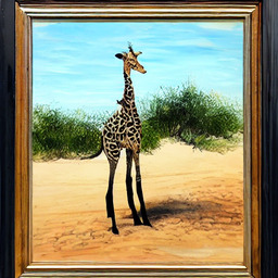
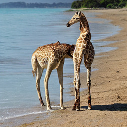
(g) (0.5CLIP(giraffe))0.5CLIPgiraffe(0.5\cdot\operatorname{CLIP}(\text{``{giraffe}''}))
+(0.5CLIP(beach))0.5CLIPbeach+(0.5\cdot\operatorname{CLIP}(\text{``{beach}''}))
Refer to caption
Refer to caption
Refer to caption
Refer to caption
(h) (0.5CLIP(bear))0.5CLIPbear(0.5\cdot\operatorname{CLIP}(\text{``{bear}''}))
+(0.5CLIP(waterfall))0.5CLIPwaterfall+(0.5\cdot\operatorname{CLIP}(\text{``{waterfall}''}))
Refer to caption
Refer to caption
Refer to caption
Refer to caption
(i) (0.5CLIP(snow))0.5CLIPsnow(0.5\cdot\operatorname{CLIP}(\text{``{snow}''}))
+(0.5CLIP(church))0.5CLIPchurch+(0.5\cdot\operatorname{CLIP}(\text{``{church}''}))
Figure 8: Images generated from sums of encodings demonstrating the realisation of both concepts in the sum

A.2.2 Leakage

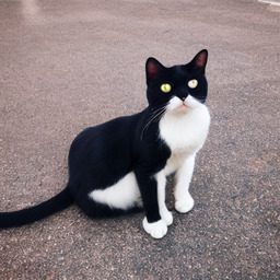
In Fig. 9 we include some images that do not fully realise both concepts, but instead allow some kind of concept “leakage” as a result of the sum. For example, the prompts “a completely black cat” and “a completely white cat”, both overwhelmingly generate images of cats of one colour, as described. The weighted sum of the two does not generate one completely white cat and one completely black cat. Instead it generates a cat that is both black and white.
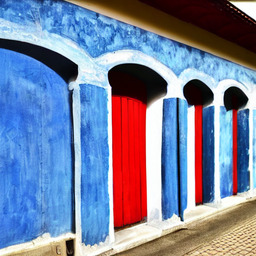
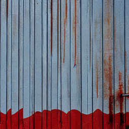
Similarly, the sum of “a wall painted red” and “a wall painted blue” does not generate a red wall and a blue wall, or even (for the majority of the time) a wall that is both red and blue. Instead, it tends to generate a wall that is one of the two colours described, but where something else in the image (such as a door) is of the other colour.
Refer to caption
Refer to caption
Refer to caption
Refer to caption
Refer to caption
Refer to caption
(a) (0.5CLIP(a completely black cat))+(0.5CLIP(a completely white cat))0.5CLIPa completely black cat0.5CLIPa completely white cat(0.5\cdot\operatorname{CLIP}(\text{``{a completely black cat}''}))\\ +(0.5\cdot\operatorname{CLIP}(\text{``{a completely white cat}''}))
Refer to caption
Refer to caption
Refer to caption
Refer to caption
Refer to caption
Refer to caption
(b) (0.5CLIP(a wall painted red))+(0.5CLIP(a wall painted blue))0.5CLIPa wall painted red0.5CLIPa wall painted blue(0.5\cdot\operatorname{CLIP}(\text{``{a wall painted red}''}))\\ +(0.5\cdot\operatorname{CLIP}(\text{``{a wall painted blue}''}))
Figure 9: Images generated from sums of encodings that demonstrate concept leakage

A.3 Sense Editing

In this section we provide more example images demonstrating the effects of our linear subspace procedure as described in § 4.

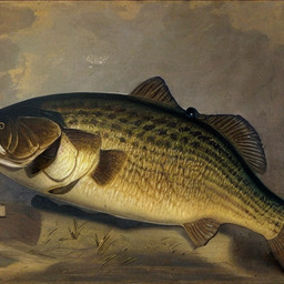
For each prompt we display 15 images sampled from the image generated from the unedited prompt encoding, alongside 15 generated from the encoding after editing it to favour each sense.
Refer to caption
Refer to caption
Refer to caption
Refer to caption
Refer to caption
Refer to caption
Refer to caption
Refer to caption
Refer to caption
Refer to caption
Refer to caption
Refer to caption
Refer to caption
Refer to caption
Refer to caption
(a) Unedited prompt encoding
Refer to caption
Refer to caption
Refer to caption
Refer to caption
Refer to caption
Refer to caption
Refer to caption
Refer to caption
Refer to caption
Refer to caption
Refer to caption
Refer to caption
Refer to caption
Refer to caption
Refer to caption
(b) Encoding edited to favour music-related sense
Refer to caption
Refer to caption
Refer to caption
Refer to caption
Refer to caption
Refer to caption
Refer to caption
Refer to caption
Refer to caption
Refer to caption
Refer to caption
Refer to caption
Refer to caption
Refer to caption
Refer to caption
(c) Encoding edited to favour fish sense
Figure 10: Prompt: “a bass
Refer to caption
Refer to caption
Refer to caption
Refer to caption
Refer to caption
Refer to caption
Refer to caption
Refer to caption
Refer to caption
Refer to caption
Refer to caption
Refer to caption
Refer to caption
Refer to caption
Refer to caption
(a) Unedited prompt encoding
Refer to caption
Refer to caption
Refer to caption
Refer to caption
Refer to caption
Refer to caption
Refer to caption
Refer to caption
Refer to caption
Refer to caption
Refer to caption
Refer to caption
Refer to caption
Refer to caption
Refer to caption
(b) Encoding edited to favour music-related sense
Refer to caption
Refer to caption
Refer to caption
Refer to caption
Refer to caption
Refer to caption
Refer to caption
Refer to caption
Refer to caption
Refer to caption
Refer to caption
Refer to caption
Refer to caption
Refer to caption
Refer to caption
(c) Encoding edited to favour fish sense
Figure 11: Prompt: “a man holding a bass
Refer to caption
Refer to caption
Refer to caption
Refer to caption
Refer to caption
Refer to caption
Refer to caption
Refer to caption
Refer to caption
Refer to caption
Refer to caption
Refer to caption
Refer to caption
Refer to caption
Refer to caption
(a) Unedited prompt encoding
Refer to caption
Refer to caption
Refer to caption
Refer to caption
Refer to caption
Refer to caption
Refer to caption
Refer to caption
Refer to caption
Refer to caption
Refer to caption
Refer to caption
Refer to caption
Refer to caption
Refer to caption
(b) Encoding edited to favour music-related sense
Refer to caption
Refer to caption
Refer to caption
Refer to caption
Refer to caption
Refer to caption
Refer to caption
Refer to caption
Refer to caption
Refer to caption
Refer to caption
Refer to caption
Refer to caption
Refer to caption
Refer to caption
(c) Encoding edited to favour fish sense
Figure 12: Prompt: “a bass displayed on a wall
Refer to caption
Refer to caption
Refer to caption
Refer to caption
Refer to caption
Refer to caption
Refer to caption
Refer to caption
Refer to caption
Refer to caption
Refer to caption
Refer to caption
Refer to caption
Refer to caption
Refer to caption
(a) Unedited prompt encoding
Refer to caption
Refer to caption
Refer to caption
Refer to caption
Refer to caption
Refer to caption
Refer to caption
Refer to caption
Refer to caption
Refer to caption
Refer to caption
Refer to caption
Refer to caption
Refer to caption
Refer to caption
(b) Encoding edited to favour animal sense
Refer to caption
Refer to caption
Refer to caption
Refer to caption
Refer to caption
Refer to caption
Refer to caption
Refer to caption
Refer to caption
Refer to caption
Refer to caption
Refer to caption
Refer to caption
Refer to caption
Refer to caption
(c) Encoding edited to favour sports-related sense
Figure 13: Prompt: “a bat
Refer to caption
Refer to caption
Refer to caption
Refer to caption
Refer to caption
Refer to caption
Refer to caption
Refer to caption
Refer to caption
Refer to caption
Refer to caption
Refer to caption
Refer to caption
Refer to caption
Refer to caption
(a) Unedited prompt encoding
Refer to caption
Refer to caption
Refer to caption
Refer to caption
Refer to caption
Refer to caption
Refer to caption
Refer to caption
Refer to caption
Refer to caption
Refer to caption
Refer to caption
Refer to caption
Refer to caption
Refer to caption
(b) Encoding edited to favour animal sense
Refer to caption
Refer to caption
Refer to caption
Refer to caption
Refer to caption
Refer to caption
Refer to caption
Refer to caption
Refer to caption
Refer to caption
Refer to caption
Refer to caption
Refer to caption
Refer to caption
Refer to caption
(c) Encoding edited to favour sports-related sense
Figure 14: Prompt: “a bat and a baseball fly through the air
Refer to caption
Refer to caption
Refer to caption
Refer to caption
Refer to caption
Refer to caption
Refer to caption
Refer to caption
Refer to caption
Refer to caption
Refer to caption
Refer to caption
Refer to caption
Refer to caption
Refer to caption
(a) Unedited prompt encoding
Refer to caption
Refer to caption
Refer to caption
Refer to caption
Refer to caption
Refer to caption
Refer to caption
Refer to caption
Refer to caption
Refer to caption
Refer to caption
Refer to caption
Refer to caption
Refer to caption
Refer to caption
(b) Encoding edited to favour animal sense
Refer to caption
Refer to caption
Refer to caption
Refer to caption
Refer to caption
Refer to caption
Refer to caption
Refer to caption
Refer to caption
Refer to caption
Refer to caption
Refer to caption
Refer to caption
Refer to caption
Refer to caption
(c) Encoding edited to favour sports-related sense
Figure 15: Prompt: “a boy holds a black bat
Refer to caption
Refer to caption
Refer to caption
Refer to caption
Refer to caption
Refer to caption
Refer to caption
Refer to caption
Refer to caption
Refer to caption
Refer to caption
Refer to caption
Refer to caption
Refer to caption
Refer to caption
(a) Unedited prompt encoding
Refer to caption
Refer to caption
Refer to caption
Refer to caption
Refer to caption
Refer to caption
Refer to caption
Refer to caption
Refer to caption
Refer to caption
Refer to caption
Refer to caption
Refer to caption
Refer to caption
Refer to caption
(b) Encoding edited to favour animal sense
Refer to caption
Refer to caption
Refer to caption
Refer to caption
Refer to caption
Refer to caption
Refer to caption
Refer to caption
Refer to caption
Refer to caption
Refer to caption
Refer to caption
Refer to caption
Refer to caption
Refer to caption
(c) Encoding edited to favour sports-related sense
Figure 16: Prompt: “a bat laying on the grass
Refer to caption
Refer to caption
Refer to caption
Refer to caption
Refer to caption
Refer to caption
Refer to caption
Refer to caption
Refer to caption
Refer to caption
Refer to caption
Refer to caption
Refer to caption
Refer to caption
Refer to caption
(a) Unedited prompt encoding
Refer to caption
Refer to caption
Refer to caption
Refer to caption
Refer to caption
Refer to caption
Refer to caption
Refer to caption
Refer to caption
Refer to caption
Refer to caption
Refer to caption
Refer to caption
Refer to caption
Refer to caption
(b) Encoding edited to favour bird sense
Refer to caption
Refer to caption
Refer to caption
Refer to caption
Refer to caption
Refer to caption
Refer to caption
Refer to caption
Refer to caption
Refer to caption
Refer to caption
Refer to caption
Refer to caption
Refer to caption
Refer to caption
(c) Encoding edited to favour construction-related sense
Figure 17: Prompt: “a crane
Refer to caption
Refer to caption
Refer to caption
Refer to caption
Refer to caption
Refer to caption
Refer to caption
Refer to caption
Refer to caption
Refer to caption
Refer to caption
Refer to caption
Refer to caption
Refer to caption
Refer to caption
(a) Unedited prompt encoding
Refer to caption
Refer to caption
Refer to caption
Refer to caption
Refer to caption
Refer to caption
Refer to caption
Refer to caption
Refer to caption
Refer to caption
Refer to caption
Refer to caption
Refer to caption
Refer to caption
Refer to caption
(b) Encoding edited to favour bird sense
Refer to caption
Refer to caption
Refer to caption
Refer to caption
Refer to caption
Refer to caption
Refer to caption
Refer to caption
Refer to caption
Refer to caption
Refer to caption
Refer to caption
Refer to caption
Refer to caption
Refer to caption
(c) Encoding edited to favour construction-related sense
Figure 18: Prompt: “a crane by the ocean
Refer to caption
Refer to caption
Refer to caption
Refer to caption
Refer to caption
Refer to caption
Refer to caption
Refer to caption
Refer to caption
Refer to caption
Refer to caption
Refer to caption
Refer to caption
Refer to caption
Refer to caption
(a) Unedited prompt encoding
Refer to caption
Refer to caption
Refer to caption
Refer to caption
Refer to caption
Refer to caption
Refer to caption
Refer to caption
Refer to caption
Refer to caption
Refer to caption
Refer to caption
Refer to caption
Refer to caption
Refer to caption
(b) Encoding edited to favour bird sense
Refer to caption
Refer to caption
Refer to caption
Refer to caption
Refer to caption
Refer to caption
Refer to caption
Refer to caption
Refer to caption
Refer to caption
Refer to caption
Refer to caption
Refer to caption
Refer to caption
Refer to caption
(c) Encoding edited to favour construction-related sense
Figure 19: Prompt: “a crane surrounded by nature
Refer to caption
Refer to caption
Refer to caption
Refer to caption
Refer to caption
Refer to caption
Refer to caption
Refer to caption
Refer to caption
Refer to caption
Refer to caption
Refer to caption
Refer to caption
Refer to caption
Refer to caption
(a) Unedited prompt encoding
Refer to caption
Refer to caption
Refer to caption
Refer to caption
Refer to caption
Refer to caption
Refer to caption
Refer to caption
Refer to caption
Refer to caption
Refer to caption
Refer to caption
Refer to caption
Refer to caption
Refer to caption
(b) Encoding edited to favour drinking-related sense
Refer to caption
Refer to caption
Refer to caption
Refer to caption
Refer to caption
Refer to caption
Refer to caption
Refer to caption
Refer to caption
Refer to caption
Refer to caption
Refer to caption
Refer to caption
Refer to caption
Refer to caption
(c) Encoding edited to favour eyeglasses sense
Figure 20: Prompt: “glasses on a table
Refer to caption
Refer to caption
Refer to caption
Refer to caption
Refer to caption
Refer to caption
Refer to caption
Refer to caption
Refer to caption
Refer to caption
Refer to caption
Refer to caption
Refer to caption
Refer to caption
Refer to caption
(a) Unedited prompt encoding
Refer to caption
Refer to caption
Refer to caption
Refer to caption
Refer to caption
Refer to caption
Refer to caption
Refer to caption
Refer to caption
Refer to caption
Refer to caption
Refer to caption
Refer to caption
Refer to caption
Refer to caption
(b) Encoding edited to favour sense of wax or official seal
Refer to caption
Refer to caption
Refer to caption
Refer to caption
Refer to caption
Refer to caption
Refer to caption
Refer to caption
Refer to caption
Refer to caption
Refer to caption
Refer to caption
Refer to caption
Refer to caption
Refer to caption
(c) Encoding edited to favour animal sense
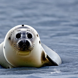
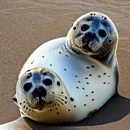
Figure 21: Prompt: “a seal
Refer to caption
Refer to caption
Refer to caption
Refer to caption
Refer to caption
Refer to caption
Refer to caption
Refer to caption
Refer to caption
Refer to caption
Refer to caption
Refer to caption
Refer to caption
Refer to caption
Refer to caption
(a) Unedited prompt encoding
Refer to caption
Refer to caption
Refer to caption
Refer to caption
Refer to caption
Refer to caption
Refer to caption
Refer to caption
Refer to caption
Refer to caption
Refer to caption
Refer to caption
Refer to caption
Refer to caption
Refer to caption
(b) Encoding edited to favour sense of wax or official seal
Refer to caption
Refer to caption
Refer to caption
Refer to caption
Refer to caption
Refer to caption
Refer to caption
Refer to caption
Refer to caption
Refer to caption
Refer to caption
Refer to caption
Refer to caption
Refer to caption
Refer to caption
(c) Encoding edited to favour animal sense
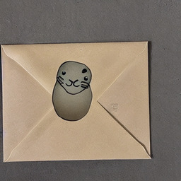
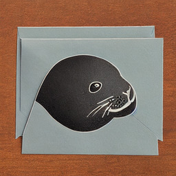
Figure 22: Prompt: “a seal on an envelope
Refer to caption
Refer to caption
Refer to caption
Refer to caption
Refer to caption
Refer to caption
Refer to caption
Refer to caption
Refer to caption
Refer to caption
Refer to caption
Refer to caption
Refer to caption
Refer to caption
Refer to caption
(a) Unedited prompt encoding
Refer to caption
Refer to caption
Refer to caption
Refer to caption
Refer to caption
Refer to caption
Refer to caption
Refer to caption
Refer to caption
Refer to caption
Refer to caption
Refer to caption
Refer to caption
Refer to caption
Refer to caption
(b) Encoding edited to favour luggage-related sense
Refer to caption
Refer to caption
Refer to caption
Refer to caption
Refer to caption
Refer to caption
Refer to caption
Refer to caption
Refer to caption
Refer to caption
Refer to caption
Refer to caption
Refer to caption
Refer to caption
Refer to caption
(c) Encoding edited to favour tree-related sense
Figure 23: Prompt: “a trunk

Appendix B Statistical Comparisons

In this section we provide detailed information about the content of the images generated in our experiments, and provide details on statistical significance testing.

B.1 Summing Encodings

The information in this section concerns the experiments described in § 3.

For each pair of prompts, 𝐬1subscript𝐬1\mathbf{s}_{1} and 𝐬2subscript𝐬2\mathbf{s}_{2}, 30 images were generated from each prompt, and 30 were generated from their weighted sum.

We were interested in the frequency with which both 𝐬1subscript𝐬1\mathbf{s}_{1} and 𝐬2subscript𝐬2\mathbf{s}_{2} were realised in an image generated by the weighted sum of their encodings. To ensure that this was not a coincidence, statistical significance was established using an unpaired permutation test where the statistic concerned was the difference between the number of images in which both prompts were realised in the images generated from the weighted sum and the images generated from each prompt alone. Some prompt pairs that we initially tried were discarded because they co-occurred too frequently in images generated by one of the prompts (for example, 𝐬1=subscript𝐬1absent\mathbf{s}_{1}=a dog in a public square” and 𝐬2=subscript𝐬2absent\mathbf{s}_{2}=a tree in a public square” were discarded because trees appear frequently in images generated by 𝐬1subscript𝐬1\mathbf{s}_{1} alone, and thus a large number of samples would have been required to establish a statistically significant difference).

All weighted sums in this section were found to realise both 𝐬1subscript𝐬1\mathbf{s}_{1} and 𝐬2subscript𝐬2\mathbf{s}_{2} more frequently than either prompt alone to a statistically significant extent (p<0.05𝑝0.05p<0.05).

Number containing:
Input Dog Lake Both Neither
CLIP(dog)CLIPdog\operatorname{CLIP}(\text{``{dog}''}) 30 0 0 0
CLIP(lake)CLIPlake\operatorname{CLIP}(\text{``{lake}''}) 0 30 0 0
0.5(CLIP(dog))+0.5(CLIP(lake))0.5CLIPdog0.5CLIPlake0.5\cdot(\operatorname{CLIP}(\text{``{dog}''}))+0.5\cdot(\operatorname{CLIP}(\text{``{lake}''})) 3 11 16 0
Table 3: Frequency of realisation of each concept for 𝐬1=subscript𝐬1absent\mathbf{s}_{1}=dog”, 𝐬2=subscript𝐬2absent\mathbf{s}_{2}=lake
Number containing:
Input Cat Tree Both Neither
CLIP(cat)CLIPcat\operatorname{CLIP}(\text{``{cat}''}) 30 0 0 0
CLIP(tree)CLIPtree\operatorname{CLIP}(\text{``{tree}''}) 0 30 0 0
0.5(CLIP(cat))+0.5(CLIP(tree))0.5CLIPcat0.5CLIPtree0.5\cdot(\operatorname{CLIP}(\text{``{cat}''}))+0.5\cdot(\operatorname{CLIP}(\text{``{tree}''})) 6 2 22 0
Table 4: Frequency of realisation of each concept for 𝐬1=subscript𝐬1absent\mathbf{s}_{1}=cat”, 𝐬2=subscript𝐬2absent\mathbf{s}_{2}=tree
Number containing:
Input Bear Hat Both Neither
CLIP(bear)CLIPbear\operatorname{CLIP}(\text{``{bear}''}) 30 0 0 0
CLIP(hat)CLIPhat\operatorname{CLIP}(\text{``{hat}''}) 0 30 0 0
0.5(CLIP(bear))+0.5(CLIP(hat))0.5CLIPbear0.5CLIPhat0.5\cdot(\operatorname{CLIP}(\text{``{bear}''}))+0.5\cdot(\operatorname{CLIP}(\text{``{hat}''})) 20 3 5 2
Table 5: Frequency of realisation of each concept for 𝐬1=subscript𝐬1absent\mathbf{s}_{1}=bear”, 𝐬2=subscript𝐬2absent\mathbf{s}_{2}=hat
Number containing:
Input Bear Waterfall Both Neither
CLIP(bear)CLIPbear\operatorname{CLIP}(\text{``{bear}''}) 30 0 0 0
CLIP(waterfall)CLIPwaterfall\operatorname{CLIP}(\text{``{waterfall}''}) 0 30 0 0
0.5(CLIP(bear))+0.5(CLIP(waterfall))0.5CLIPbear0.5CLIPwaterfall0.5\cdot(\operatorname{CLIP}(\text{``{bear}''}))+0.5\cdot(\operatorname{CLIP}(\text{``{waterfall}''})) 10 12 6 2
Table 6: Frequency of realisation of each concept for 𝐬1=subscript𝐬1absent\mathbf{s}_{1}=bear”, 𝐬2=subscript𝐬2absent\mathbf{s}_{2}=waterfall
Number containing:
Input Elephant Snow Both Neither
CLIP(elephant)CLIPelephant\operatorname{CLIP}(\text{``{elephant}''}) 30 0 0 0
CLIP(snow)CLIPsnow\operatorname{CLIP}(\text{``{snow}''}) 0 30 0 0
0.5(CLIP(elephant))+0.5(CLIP(snow))0.5CLIPelephant0.5CLIPsnow0.5\cdot(\operatorname{CLIP}(\text{``{elephant}''}))+0.5\cdot(\operatorname{CLIP}(\text{``{snow}''})) 7 3 20 0
Table 7: Frequency of realisation of each concept for 𝐬1=subscript𝐬1absent\mathbf{s}_{1}=elephant”, 𝐬2=subscript𝐬2absent\mathbf{s}_{2}=snow
Number containing:
Input Giraffe Beach Both Neither
CLIP(giraffe)CLIPgiraffe\operatorname{CLIP}(\text{``{giraffe}''}) 30 0 0 0
CLIP(beach)CLIPbeach\operatorname{CLIP}(\text{``{beach}''}) 0 30 0 0
0.5(CLIP(giraffe))+0.5(CLIP(beach))0.5CLIPgiraffe0.5CLIPbeach0.5\cdot(\operatorname{CLIP}(\text{``{giraffe}''}))+0.5\cdot(\operatorname{CLIP}(\text{``{beach}''})) 3 17 9 1
Table 8: Frequency of realisation of each concept for 𝐬1=subscript𝐬1absent\mathbf{s}_{1}=giraffe”, 𝐬2=subscript𝐬2absent\mathbf{s}_{2}=beach
Number containing:
Input Goat Crown Both Neither
CLIP(goat)CLIPgoat\operatorname{CLIP}(\text{``{goat}''}) 30 0 0 0
CLIP(crown)CLIPcrown\operatorname{CLIP}(\text{``{crown}''}) 0 30 0 0
0.5(CLIP(goat))+0.5(CLIP(crown))0.5CLIPgoat0.5CLIPcrown0.5\cdot(\operatorname{CLIP}(\text{``{goat}''}))+0.5\cdot(\operatorname{CLIP}(\text{``{crown}''})) 11 4 11 4
Table 9: Frequency of realisation of each concept for 𝐬1=subscript𝐬1absent\mathbf{s}_{1}=goat”, 𝐬2=subscript𝐬2absent\mathbf{s}_{2}=crown
Number containing:
Input Snow Church Both Neither
CLIP(snow)CLIPsnow\operatorname{CLIP}(\text{``{snow}''}) 30 0 0 0
CLIP(church)CLIPchurch\operatorname{CLIP}(\text{``{church}''}) 0 30 0 0
0.5(CLIP(snow))+0.5(CLIP(church))0.5CLIPsnow0.5CLIPchurch0.5\cdot(\operatorname{CLIP}(\text{``{snow}''}))+0.5\cdot(\operatorname{CLIP}(\text{``{church}''})) 14 1 15 0
Table 10: Frequency of realisation of each concept for 𝐬1=subscript𝐬1absent\mathbf{s}_{1}=snow”, 𝐬2=subscript𝐬2absent\mathbf{s}_{2}=church
Number containing:
Input Tiger Glasses Both Neither
CLIP(tiger)CLIPtiger\operatorname{CLIP}(\text{``{tiger}''}) 30 0 0 0
CLIP(glasses)CLIPglasses\operatorname{CLIP}(\text{``{glasses}''}) 0 30 0 0
0.5(CLIP(tiger))+0.5(CLIP(glasses))0.5CLIPtiger0.5CLIPglasses0.5\cdot(\operatorname{CLIP}(\text{``{tiger}''}))+0.5\cdot(\operatorname{CLIP}(\text{``{glasses}''})) 21 1 8 0
Table 11: Frequency of realisation of each concept for 𝐬1=subscript𝐬1absent\mathbf{s}_{1}=tiger”, 𝐬2=subscript𝐬2absent\mathbf{s}_{2}=glasses

B.2 Sense Editing

The information in this section concerns the experiments described in § 4.

For each prompt, 𝐬𝐬\mathbf{s}, 30 images were generated from the unedited prompt encoding and 30 each were generated from the version edited to favour each sense.
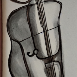
We were interested in the frequency with which the intended sense was the only sense realised in an image generated by the one of the edited encodings. The value for the targeted sense of an edited encoding is bolded if it was found to be a statistically significant increase of realisation of that sense when compared to the unedited encoding. Statistical significance was established using an unpaired permutation test where the statistic concerned was the difference between the number of images in which the intended sense was realised, between images generated by the edited encoding and the unedited encoding. The significance level used in these experiments was p<0.05𝑝0.05p<0.05.

Table 12, table 13 and table 14 concern prompts including the word “bass”, where Sense 1 is a type of musical instrument (for counting purposes we included all kinds of instruments that can be described as a “bass”) and Sense 2 is a type of fish.

Sense 1 Sense 2 Both Neither
Unedited 16 14 0 0
Edited ( \rightarrow Sense 1) 29 1 0 0
Edited ( \rightarrow Sense 2) 3 27 0 0
Table 12: Frequency of realisation of each concept for 𝐬=𝐬absent\mathbf{s}=a bass” from the unedited prompt encoding, and encodings edited to favour each sense.
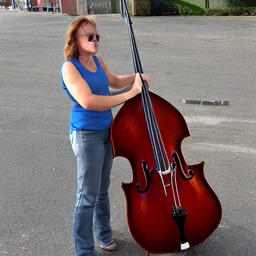
Sense 1 Sense 2 Both Neither
Unedited 10 19 1 0
Edited ( \rightarrow Sense 1) 24 2 0 4
Edited ( \rightarrow Sense 2) 0 30 0 0
Table 13: Frequency of realisation of each concept for 𝐬=𝐬absent\mathbf{s}=a man holds a bass” from the unedited prompt encoding, and encodings edited to favour each sense.
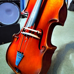
Sense 1 Sense 2 Both Neither
Unedited 23 5 0 2
Edited ( \rightarrow Sense 1) 30 0 0 0
Edited ( \rightarrow Sense 2) 4 25 0 1
Table 14: Frequency of realisation of each concept for 𝐬=𝐬absent\mathbf{s}=a bass is displayed on a wall” from the unedited prompt encoding, and encodings edited to favour each sense.

Table 15, table 16, table 17 and table 18 concern prompts that include the ambiguous word “bat”, for which Sense 1 is a winged nocturnal mammal, and Sense 2 is a piece of equipment used to play sports such as baseball.

Sense 1 Sense 2 Both Neither
Unedited 30 0 0 0
Edited ( \rightarrow Sense 1) 30 0 0 0
Edited ( \rightarrow Sense 2) 2 16 8 4
Table 15: Frequency of realisation of each concept for 𝐬=𝐬absent\mathbf{s}=a bat” from the unedited prompt encoding, and encodings edited to favour each sense.
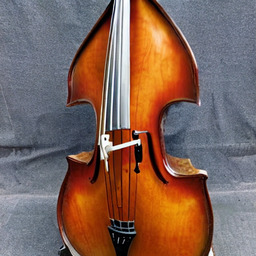
Sense 1 Sense 2 Both Neither
Unedited 22 4 2 2
Edited ( \rightarrow Sense 1) 27 0 1 2
Edited ( \rightarrow Sense 2) 1 24 3 2
Table 16: Frequency of realisation of each concept for 𝐬=𝐬absent\mathbf{s}=a bat and a baseball fly through the air” from the unedited prompt encoding, and encodings edited to favour each sense.
Sense 1 Sense 2 Both Neither
Unedited 4 17 4 5
Edited ( \rightarrow Sense 1) 18 3 5 4
Edited ( \rightarrow Sense 2) 0 27 0 3
Table 17: Frequency of realisation of each concept for 𝐬=𝐬absent\mathbf{s}=a boy holds a black bat” from the unedited prompt encoding, and encodings edited to favour each sense.
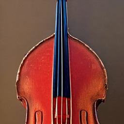
Sense 1 Sense 2 Both Neither
Unedited 30 0 0 0
Edited ( \rightarrow Sense 1) 30 0 0 0
Edited ( \rightarrow Sense 2) 2 18 3 7
Table 18: Frequency of realisation of each concept for 𝐬=𝐬absent\mathbf{s}=a bat laying on the grass” from the unedited prompt encoding, and encodings edited to favour each sense.
Table 19, table 20 and table 21 all include the ambiguous word “crane”, for which Sense 1 is a long-legged bird, and Sense 2 is a piece of machinery often used in construction.

Sense 1 Sense 2 Both Neither
Unedited 24 4 2 0
Edited ( \rightarrow Sense 1) 29 0 0 1
Edited ( \rightarrow Sense 2) 10 18 2 0
Table 19: Frequency of realisation of each concept for 𝐬=𝐬absent\mathbf{s}=a crane” from the unedited prompt encoding, and encodings edited to favour each sense.
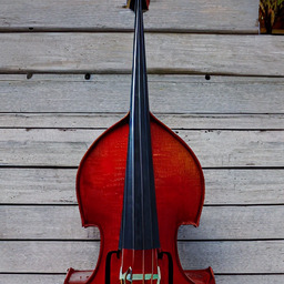
Sense 1 Sense 2 Both Neither
Unedited 19 9 1 1
Edited ( \rightarrow Sense 1) 27 1 0 2
Edited ( \rightarrow Sense 2) 1 28 1 0
Table 20: Frequency of realisation of each concept for 𝐬=𝐬absent\mathbf{s}=a crane by the ocean” from the unedited prompt encoding, and encodings edited to favour each sense.
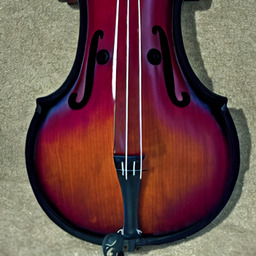
Sense 1 Sense 2 Both Neither
Unedited 9 16 5 0
Edited ( \rightarrow Sense 1) 24 4 1 1
Edited ( \rightarrow Sense 2) 1 29 0 0
Table 21: Frequency of realisation of each concept for 𝐬=𝐬absent\mathbf{s}=a crane surrounded by nature” from the unedited prompt encoding, and encodings edited to favour each sense.
Table 22 gives results for the prompt “glasses on a table”, where Sense 1 of “glasses” refers to glasses used for drinking, and Sense 2 refers to eyeglasses.

Sense 1 Sense 2 Both Neither
Unedited 8 21 1 0
Edited ( \rightarrow Sense 1) 24 3 0 3
Edited ( \rightarrow Sense 2) 0 29 0 1
Table 22: Frequency of realisation of each concept for 𝐬=𝐬absent\mathbf{s}=glasses on a table” from the unedited prompt encoding, and encodings edited to favour each sense.
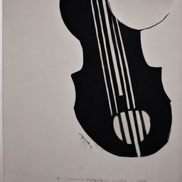
Table 23 and table 24 give results for prompts containing the word “seal”, where Sense 1 refers to a wax seal or an official seal on a letter or document, and Sense 2 refers to a marine mammal.

Sense 1 Sense 2 Both Neither
Unedited 2 22 6 0
Edited ( \rightarrow Sense 1) 26 0 4 0
Edited ( \rightarrow Sense 2) 0 30 0 0
Table 23: Frequency of realisation of each concept for 𝐬=𝐬absent\mathbf{s}=a seal” from the unedited prompt encoding, and encodings edited to favour each sense.
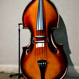
Sense 1 Sense 2 Both Neither
Unedited 0 25 2 3
Edited ( \rightarrow Sense 1) 21 1 7 1
Edited ( \rightarrow Sense 2) 0 30 0 0
Table 24: Frequency of realisation of each concept for 𝐬=𝐬absent\mathbf{s}=a seal on an envelope” from the unedited prompt encoding, and encodings edited to favour each sense.
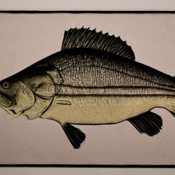
Table 25 provides results for the prompt “a trunk” where Sense 1 of “trunk” refers to a box used as luggage (for counting purposes, the trunk of a car was also included in this sense) and Sense 2 refers to the trunk of a tree.

Sense 1 Sense 2 Both Neither
Unedited 15 13 2 0
Edited ( \rightarrow Sense 1) 30 0 0 0
Edited ( \rightarrow Sense 2) 0 28 2 0
Table 25: Frequency of realisation of each concept for 𝐬=𝐬absent\mathbf{s}=a trunk” from the unedited prompt encoding, and encodings edited to favour each sense.
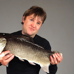
Appendix C Sentences Used to Find Meaning Directions

Here we provide the sentences 𝐬ambsuperscript𝐬amb\mathbf{s}^{{\color[rgb]{0.5625,0.3671875,0.61328125}\definecolor[named]{pgfstrokecolor}{rgb}{0.5625,0.3671875,0.61328125}\text{amb}}}, 𝐬(1)superscript𝐬1\mathbf{s}^{{\color[rgb]{0.390625,0.5859375,0.9296875}\definecolor[named]{pgfstrokecolor}{rgb}{0.390625,0.5859375,0.9296875}(1)}} and 𝐬(2)superscript𝐬2\mathbf{s}^{{\color[rgb]{0.73046875,0.15234375,0.2890625}\definecolor[named]{pgfstrokecolor}{rgb}{0.73046875,0.15234375,0.2890625}(2)}} that were used to calculate difference subspaces and meaning directions for each of the words we used.
𝐬ambsuperscript𝐬amb\mathbf{s}^{{\color[rgb]{0.5625,0.3671875,0.61328125}\definecolor[named]{pgfstrokecolor}{rgb}{0.5625,0.3671875,0.61328125}\text{amb}}} 𝐬(1)superscript𝐬1\mathbf{s}^{{\color[rgb]{0.390625,0.5859375,0.9296875}\definecolor[named]{pgfstrokecolor}{rgb}{0.390625,0.5859375,0.9296875}(1)}} 𝐬(2)superscript𝐬2\mathbf{s}^{{\color[rgb]{0.73046875,0.15234375,0.2890625}\definecolor[named]{pgfstrokecolor}{rgb}{0.73046875,0.15234375,0.2890625}(2)}}
a bass a double bass a sea bass
there is a bass there is a double bass there is a sea bass
the person saw a bass the musician played a double bass the fisherman caught a sea bass
a person mentions a bass a musician plays a double bass an angler holds a sea bass
a nearby location has a bass a jazz band has a double bass a local aquarium has a sea bass
Table 26: Sentences used to find meaning directions for “bass
𝐬ambsuperscript𝐬amb\mathbf{s}^{{\color[rgb]{0.5625,0.3671875,0.61328125}\definecolor[named]{pgfstrokecolor}{rgb}{0.5625,0.3671875,0.61328125}\text{amb}}} 𝐬(1)superscript𝐬1\mathbf{s}^{{\color[rgb]{0.390625,0.5859375,0.9296875}\definecolor[named]{pgfstrokecolor}{rgb}{0.390625,0.5859375,0.9296875}(1)}} 𝐬(2)superscript𝐬2\mathbf{s}^{{\color[rgb]{0.73046875,0.15234375,0.2890625}\definecolor[named]{pgfstrokecolor}{rgb}{0.73046875,0.15234375,0.2890625}(2)}}
a bat a fruit bat a baseball bat
there is a bat there is a fruit bat there is a baseball bat
i do things with the bat i feed insects to the fruit bat i play baseball with the baseball bat
the person saw a bat the boy saw a fruit bat the boy bought a baseball bat
a person mentions a bat a wildlife expert feeds a fruit bat a baseball player swings a baseball bat
a bat is laying on the floor a fruit bat is hanging from the tree a baseball bat is laying on the base
a bat in a box a fruit bat in a cave a baseball bat in a store
a nearby location has a bat a local zoo keeps an fruit bat a sports store sells a baseball bat
Table 27: Sentences used to find meaning directions for “bat
𝐬ambsuperscript𝐬amb\mathbf{s}^{{\color[rgb]{0.5625,0.3671875,0.61328125}\definecolor[named]{pgfstrokecolor}{rgb}{0.5625,0.3671875,0.61328125}\text{amb}}} 𝐬(1)superscript𝐬1\mathbf{s}^{{\color[rgb]{0.390625,0.5859375,0.9296875}\definecolor[named]{pgfstrokecolor}{rgb}{0.390625,0.5859375,0.9296875}(1)}} 𝐬(2)superscript𝐬2\mathbf{s}^{{\color[rgb]{0.73046875,0.15234375,0.2890625}\definecolor[named]{pgfstrokecolor}{rgb}{0.73046875,0.15234375,0.2890625}(2)}}
a crane a sandhill crane a tower crane
there is a crane there is a sandhill crane there is a tower crane
there is a crane on the other side there is a sandhill crane on the nature reserve there is a tower crane on the building site
a crane is tall a sandhill crane hunts fish a tower crane lifts loads
a boy sees a crane a boy feeds a sandhill crane a man operates a tower crane
a crane beside a tree a sandhill crane beside a nest a tower crane beside a bulldozer
a crane is casting a shadow a sandhill crane is eating some fish a tower crane is lifting a container
a crane by the ocean a sandhill crane in a nest a tower crane in a quarry
Table 28: Sentences used to find meaning directions for “crane
𝐬ambsuperscript𝐬amb\mathbf{s}^{{\color[rgb]{0.5625,0.3671875,0.61328125}\definecolor[named]{pgfstrokecolor}{rgb}{0.5625,0.3671875,0.61328125}\text{amb}}} 𝐬(1)superscript𝐬1\mathbf{s}^{{\color[rgb]{0.390625,0.5859375,0.9296875}\definecolor[named]{pgfstrokecolor}{rgb}{0.390625,0.5859375,0.9296875}(1)}} 𝐬(2)superscript𝐬2\mathbf{s}^{{\color[rgb]{0.73046875,0.15234375,0.2890625}\definecolor[named]{pgfstrokecolor}{rgb}{0.73046875,0.15234375,0.2890625}(2)}}
glasses wine glasses reading glasses
there are glasses there are wine glasses there are reading glasses
the person saw glasses the waiter filled wine glasses the scientist wore reading glasses
a person holds glasses a waiter fills wine glasses a scientist wears reading glasses
glasses are being used wine glasses are being cleaned reading glasses are being cleaned
Table 29: Sentences used to find meaning directions for “glasses
𝐬ambsuperscript𝐬amb\mathbf{s}^{{\color[rgb]{0.5625,0.3671875,0.61328125}\definecolor[named]{pgfstrokecolor}{rgb}{0.5625,0.3671875,0.61328125}\text{amb}}} 𝐬(1)superscript𝐬1\mathbf{s}^{{\color[rgb]{0.390625,0.5859375,0.9296875}\definecolor[named]{pgfstrokecolor}{rgb}{0.390625,0.5859375,0.9296875}(1)}} 𝐬(2)superscript𝐬2\mathbf{s}^{{\color[rgb]{0.73046875,0.15234375,0.2890625}\definecolor[named]{pgfstrokecolor}{rgb}{0.73046875,0.15234375,0.2890625}(2)}}
a seal a wax seal a harp seal
there is a seal there is a wax seal there is a harp seal
the person saw a seal the postmaster stamped a wax seal the zookeeper fed a harp seal
a person mentions a seal a butler opens a wax seal a boy pets a harp seal
a seal in a frame a wax seal on an envelope a harp seal in the ocean
a nearby location has a seal a fancy letter has a wax seal a large zoo has a harp seal
Table 30: Sentences used to find meaning directions for “seal
𝐬ambsuperscript𝐬amb\mathbf{s}^{{\color[rgb]{0.5625,0.3671875,0.61328125}\definecolor[named]{pgfstrokecolor}{rgb}{0.5625,0.3671875,0.61328125}\text{amb}}} 𝐬(1)superscript𝐬1\mathbf{s}^{{\color[rgb]{0.390625,0.5859375,0.9296875}\definecolor[named]{pgfstrokecolor}{rgb}{0.390625,0.5859375,0.9296875}(1)}} 𝐬(2)superscript𝐬2\mathbf{s}^{{\color[rgb]{0.73046875,0.15234375,0.2890625}\definecolor[named]{pgfstrokecolor}{rgb}{0.73046875,0.15234375,0.2890625}(2)}}
a trunk a storage trunk a tree trunk
there is a trunk there is a storage trunk there is a tree trunk
the person saw a trunk the traveller carried a storage trunk the lumberjack sawed a tree trunk
a person mentions a trunk a passenger carries a storage trunk a carpenter uses a tree trunk
a trunk is being used a storage trunk is being packed a tree trunk is being felled
Table 31: Sentences used to find meaning directions for “trunk