Asynchronous global-local non-invasive coupling
for linear elliptic problems

Abstract

This paper presents the first asynchronous version of the Global/Local non-invasive coupling, capable of dealing efficiently with multiple, possibly adjacent, patches. We give a new interpretation of the coupling in terms of primal domain decomposition method, and we prove the convergence of the relaxed asynchronous iteration. The asynchronous paradigm lifts many bottlenecks of the Global/Local coupling performance. We illustrate the method on several linear elliptic problems as encountered in thermal and elasticity studies.

1 Introduction

Engineering problems are often defined on very different scales, ranging from a coarse scale to model the whole structure to very fine scales that allow for the local details to be resolved. A method frequently used in the industry to link the scales is the submodeling [33, 50, 12]. This non-intrusive method is simple to implement but has shown limits regarding the accuracy of the results.

The non-invasive Global-Local coupling technique was first proposed and implemented in [22]. It aims at making submodeling accurate by means of iterations. It extends some previous reanalysis techniques [32, 56, 57], and it has strong connections with Schwarz domain decomposition methods [29, 26] and multiscale methods [36] while preserving the non-intrusive character of submodeling. Thus, it was implemented to couple research codes and legacy commercial software like Abaqus [6], Code_Aster [15], or Z-set [55].

The philosophy is to start from a simplified global model and then allow local alterations (geometry, material, load, and mesh) to be inserted and their effect to be evaluated without heavy intervention on the initial model (see [1] for a pedagogic presentation). It was successfully applied in many contexts like the introduction of local plasticity and geometrical refinements [22], the computation of the propagation of cracks in a sound model [15], the evaluation of stochastic effects with deterministic computations [9, 47], the taking into account of the exact geometry of connectors in an assembly of plates [28]. In [15] the method was used in order to implement a nonlinear domain decomposition method [34, 13, 30, 46] in a non-invasive manner in Code_Aster. Extension of the approach to explicit dynamics was proposed in [3], improved in [4] and applied to the prediction of delamination under impact loading in [5].

All the above applications were developed in a synchronous framework that has been taken advantage of by accelerators (Aitken, quasi-Newton, Krylov), see [26] where the method is proved to be an implementation of an alternating Dirichlet-Robin approach where the Robin parameter corresponds to the condensation of the coarse domain covered by the patch. However, due to the alternating nature of the method, its computational performance is inherently limited, with some processors idling while others are computing. This paper aims at deriving an asynchronous version of the global-local coupling, which enables us to get rid of most waiting periods.

Asynchronous iteration was introduced in [8], under the name of chaotic relaxation, to solve large linear systems. It has subsequently been the subject of several studies, [44] generalized the method to nonlinear problems, the work in [2] allowed the first implementation of asynchronous methods on multiprocessor architectures, in [17, 49] convergence results for the asynchronous iterations based on the notion of classical contraction was presented, recent work in [10] show interesting theoretical and practical results for the Richardson iterations from the asynchronous point of view.

Several works have shown that domain decomposition methods are well suited for asynchronous parallel computation, such as alternating Schwarz [54], optimized Schwarz [39, 59, 7], sub-structuring methods [38, 20], primal Schur domain decomposition method [21] and also multigrid methods [58]. In [53, 19], one can find a global review of asynchronous iterations from both theoretical and implementation points of view.

Our study is conducted on linear elliptic problems discretized by the finite element approach. We prove the convergence of relaxed iterations using the theory of paracontractions [16], and illustrate it on several examples of thermal and elasticity problems.

The paper is organized as follows: in Section 2 a new derivation of the method is proposed, in Section 3 the asynchronous framework is exposed and studied, illustrations are given in Section 4.

2 The non-invasive global/local coupling

The framework chosen to develop the method is the one of linear elliptic problems. This corresponds to certain thermal or elasticity static problems. We propose to derive the method as an evolution of the submodeling technique, we also give another (original) interpretation in terms of domain decomposition method.

2.1 Principle of the method

(a) Global problem

(b) Refined zones of interest

(c) Reference problem

Figure 1: Models and subdomains for the Global/Local coupling

(a) Global solution

(b) Submodeling solution

(c) Reference solution

Figure 2: Comparison of the norm of the heat flux for the submodeling and reference approaches (thermal problem)

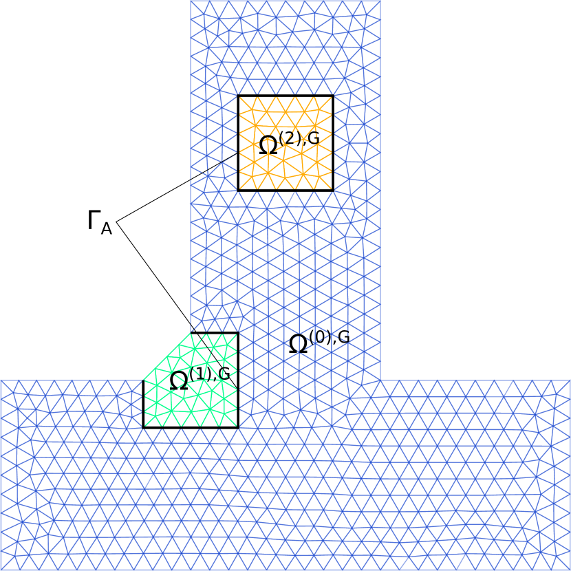
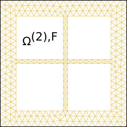
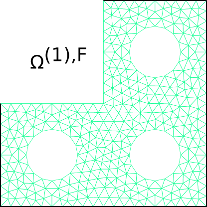
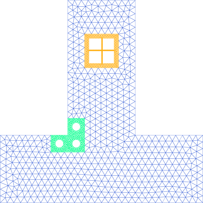
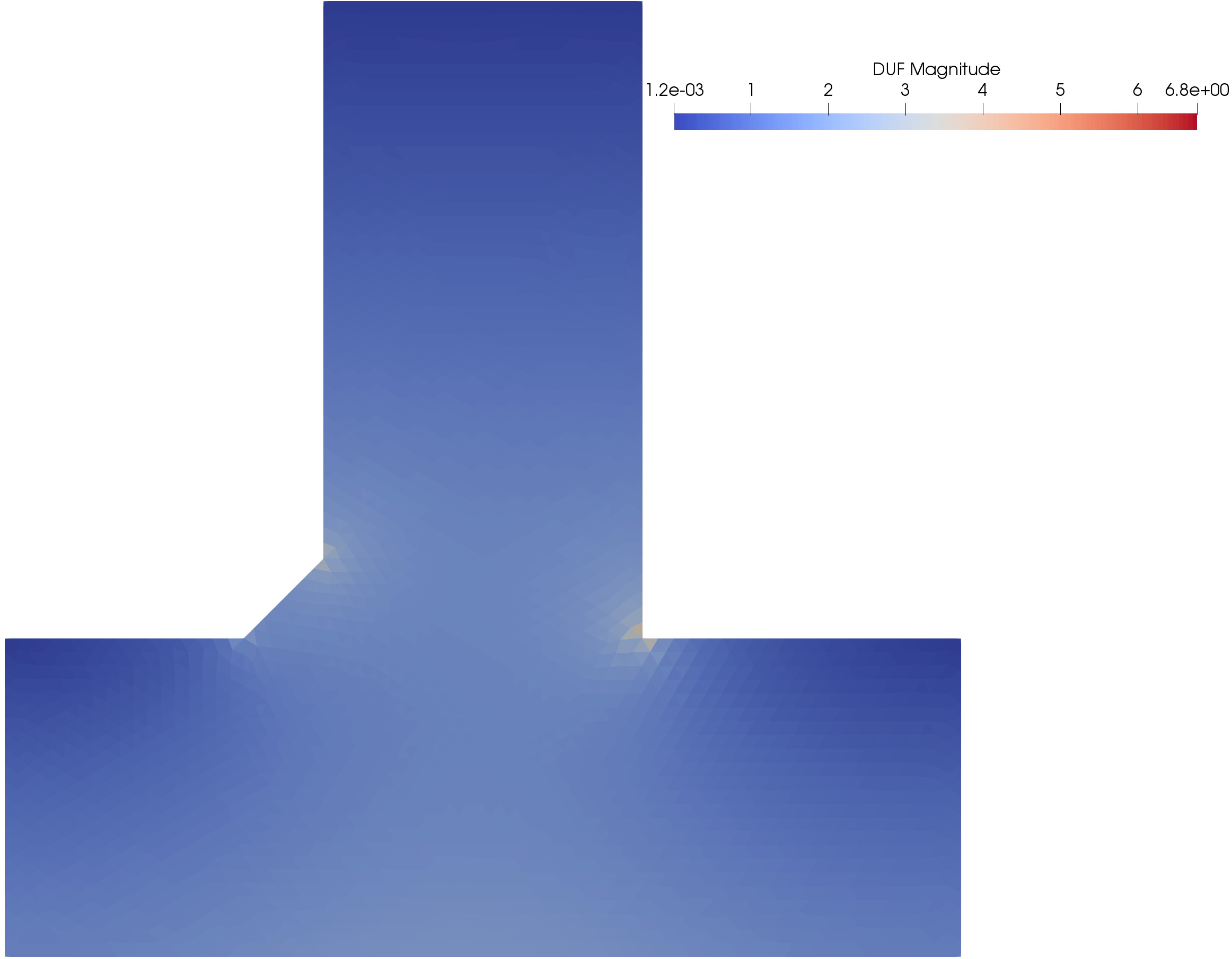
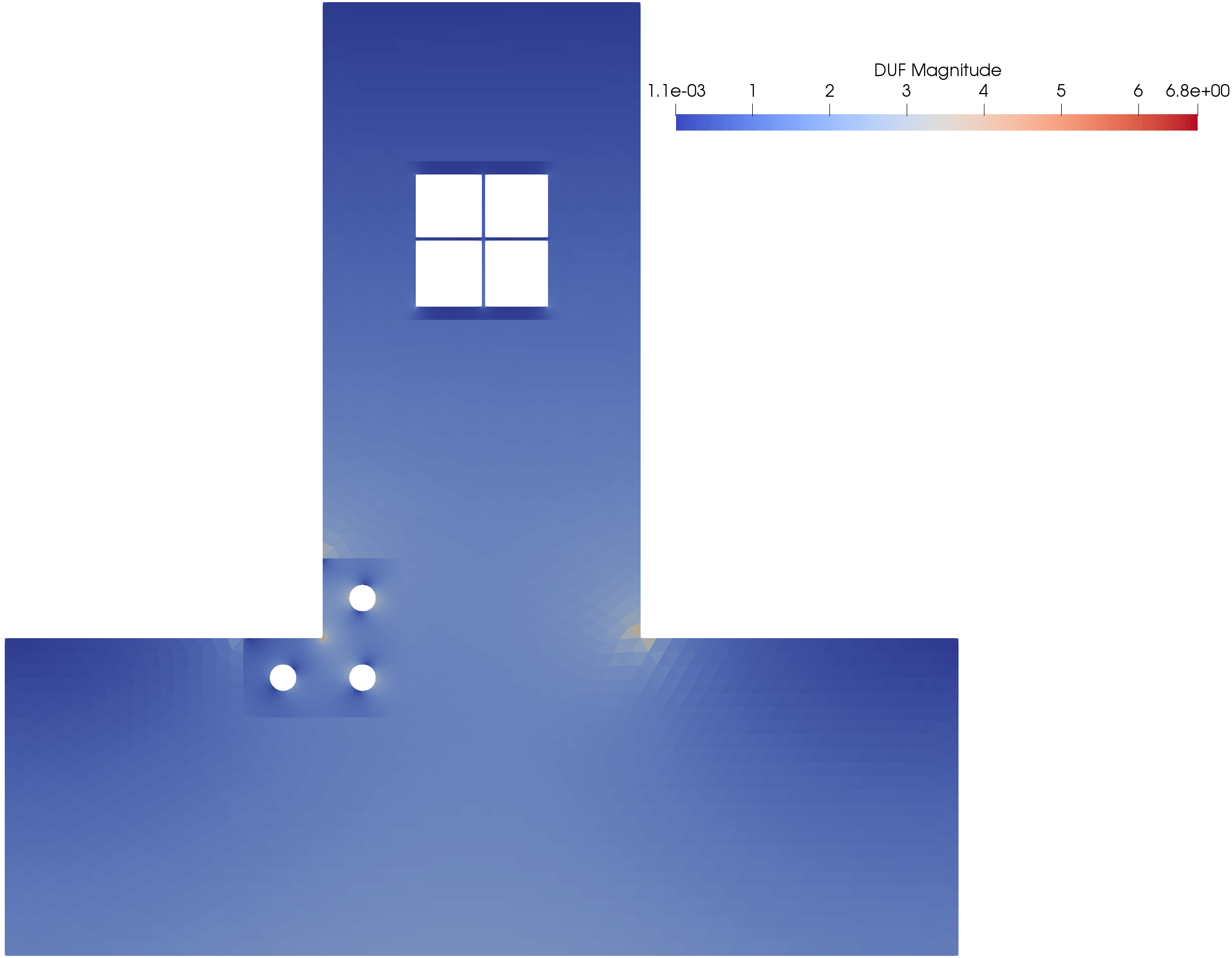
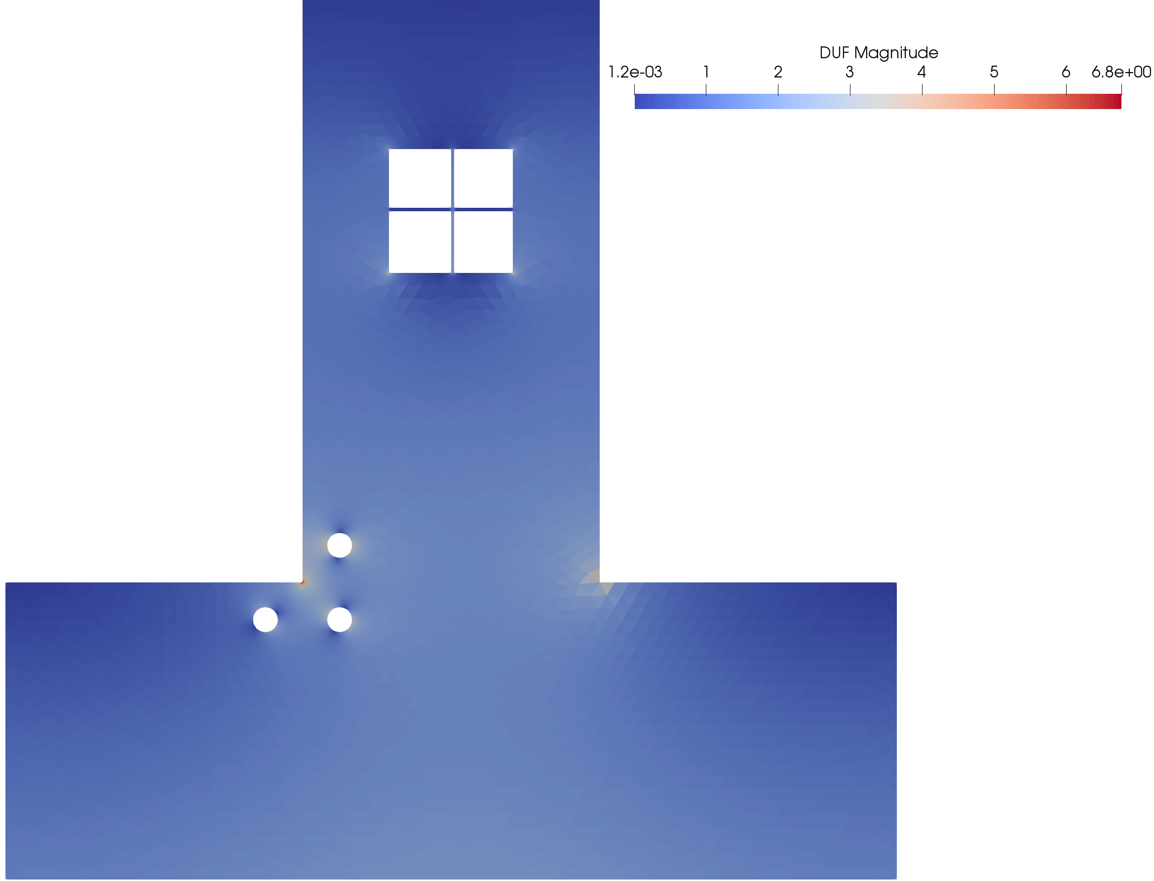
The classical scenario is illustrated on Figure 1. A linear Global coarse model is used to describe a large structure. After the initial computation (Figure 2(a)), some zones of interest $\Omega^{s,G}$ $(s>0)$ are selected because some criterion has been exceeded or because it was known from the beginning that some details were missing in the Global model. This is the case for our illustration where geometrical details and adapted meshes are introduced in the Fine modeling of the zones of interest $\Omega^{s,F}$. Material laws could also be modified by the introduction of some heterogeneity. Fine computations are run in parallel on the patches using the Global solution as Dirichlet boundary condition (for $s>0$, the interior of the Fine and Global subdomains may differ, but their interface $\Gamma^{s}$ must be the same $\Gamma^{s}=\Omega\cap\partial\Omega^{s,G}=\Omega\cap\partial\Omega^{s,F}$).

This sequence of computations corresponds to the (in)famous submodeling technique which is known to result in large errors because the effects of Fine patches are not sent back to the Global model, and interactions between patches are thus impossible to be accounted for.

The error can be materialized by the lack of balance of the fluxes between the Global zone not covered by patches, denoted by $\Omega^{0}$ and the Fine models. As can be seen on Figure 2(b), which shows the norm of the heat flux and where the Fine models overwrite the Global ones. There is a discontinuity at the interface which does not exist in the Reference computation where all interactions are taken into account; see Figure 2(c) which corresponds to a direct computation of the Reference model where the zones of interest are described with the Fine models, see Figure 1(c).

The Global/Local coupling is a simple iterative technique (a Richardson iteration for its simpler version) aiming at obtaining the Reference solution from computations carried on the Global and Fine models (that is to say without the potentially cumbersome creation of the Reference model) with minimal intervention on the models and software.

2.2 Derivation of the Global/Local coupling

There exist many ways to derive the Global/Local coupling. This subsection just sets up the method, the convergence of the asynchronous iteration being the subject of the next section.

We use boldface for discrete (nodal) quantities, lower case for vectors and upper case for matrices.

2.2.1 Global problem

The Global problem is the classical finite element discretization of a coarse model of the structure, with one extra interface load. Let $\mathbf{p}_{\Gamma}$ denote the vector of nodal fluxes applied on the interface nodes $\Gamma=\bigcup_{s=0}^{N}\Gamma^{s}$. To position the interface in the Global domain we introduce the boolean trace operator $\mathbf{T}^{G}:\Omega^{G}\to\Gamma$, its transpose is the extension-by-0 operator.

The discrete Global problem can be written as:

$$\left|\begin{aligned} &\text{For given }\mathbf{p}_{\Gamma}\text{ on }\Gamma,\text{ find }\mathbf{u}^{G}\text{ in }\Omega^{G},\text{ such that}\\ &\mathbf{K}^{G}\mathbf{u}^{G}=\mathbf{f}^{G}+\mathbf{T}^{G^{T}}\mathbf{p}_{\Gamma}\end{aligned}\right.$$ (1)

where one can recognize the symmetric definite positive stiffness matrix $\mathbf{K}^{G}$, the vector of generalized loads $\mathbf{f}^{G}$, the vector of unknowns $\mathbf{u}^{G}$.

The interface load is non-standard since it is a Neumann condition applied on an immersed surface. This corresponds to imposing a flux discontinuity in the Global model. It appears that such a load can easily be applied in industrial software, and the Global solution is obtained with a classical solver.

In order to single out the contribution of subdomains, we introduce the boolean assembly operators $\mathbf{A}^{s}:\ \Gamma^{s,G}\to\Gamma^{G}$ as classically encountered in the primal domain decomposition methods, see [27] for instance. Their transpose enables us to restrict some Global interface data to the boundary of a subdomain.

2.2.2 Fine problems

The Fine problems are set on the discretized subdomains $\Omega^{s,F}$. Boolean matrix $\mathbf{T}^{s,F}$ is the trace operator on the Fine mesh $\Omega^{s,F}\to\Gamma^{s,F}$. For a good matching of the models, the interface is assumed to suit edges of the Fine elements. Anyhow, we do not require matching Global and Fine discretization, and we introduce Global-to-Fine transfer matrix $\mathbf{J}^{s}$ which enables us to define Fine Dirichlet problems with boundary conditions coming from the Global model.

The fine problems can be written as:

$$\left|\begin{aligned} &\text{Given }\mathbf{u}^{G}_{\Gamma}\text{ on }\Gamma;\forall s>0,\text{ find }\mathbf{u}^{s,F}\text{ in }\Omega^{s,F}\text{ and }\boldsymbol{\lambda}^{s,F}\text{ on }\Gamma^{s}\text{ such that}\\ &\mathbf{K}^{s,F}\mathbf{u}^{s,F}+\mathbf{f}^{s,F}=\mathbf{T}^{s,F^{T}}\boldsymbol{\lambda}^{s,F}\\ &\mathbf{T}^{s,F}\mathbf{u}^{s,F}=\mathbf{J}^{s}\mathbf{A}^{s^{T}}\mathbf{u}^{G}_{\Gamma}\\ \end{aligned}\right.$$ (2)

2.2.3 Reference problem

The Reference problem is the collection of Fine problems connected to the same interface displacement $\mathbf{u}^{G}_{\Gamma}$ and such that the nodal reactions are in balance once projected back on the Global interface.

First, we need to clarify the role played by Subdomain $0$, which might be non-existent. It is a subdomain, sometimes called Complement domain in the Global/Local literature, where the Fine and Global model coincide (same geometry $\Omega^{0}$, same properties, same load, same approximation). Its main role is to help process the nodal reaction $\boldsymbol{\lambda}^{0}$:

$$\boldsymbol{\lambda}^{0}=\mathbf{T}^{0}(\mathbf{K}^{0}\mathbf{u}^{0}-\mathbf{f}^{0})$$ (3)

We are now in position to formulate the Reference problem:

$$\left|\begin{aligned} &\text{Find }\mathbf{u}^{G}_{\Gamma}\text{ on }\Gamma\text{ s.t }\\ &\mathbf{r}_{\Gamma}:=-\left(\mathbf{A}^{0}\boldsymbol{\lambda}^{0}+\sum_{s=1}^{N}\mathbf{A}^{s}\mathbf{J}^{s^{T}}\boldsymbol{\lambda}^{s,F}\right)=0\\ &\text{ where the reactions are obtained from}~{}\eqref{eq:sdF}\text{ and}~{}\eqref{eq:sd0}.\end{aligned}\right.$$ (4)

2.2.4 Condensed problems

As usual with domain decomposition methods, the process is fully driven by the convergence of interface quantities. For the analysis of the method, it is thus convenient to condense these previous problems at the interface.

We then deduce from the system 2 the Dirichlet-to-Neumann operator for the Fine problems which can be written as:

$$\boldsymbol{\lambda}^{s,F}=\mathbf{S}^{s,F}\mathbf{u}^{s,F}_{\Gamma}-\mathbf{b}^{s,F}\\$$ (5)

With:

$$\begin{cases}\mathbf{S}^{s,F}&=\mathbf{K}^{s,F}_{\Gamma\Gamma}-\mathbf{K}^{s,F}_{\Gamma i}\mathbf{K}^{s,F^{-1}}_{ii}\mathbf{K}^{s,F}_{i\Gamma}\\ \mathbf{b}^{s,F}&=\mathbf{f}^{s,F}_{\Gamma}-\mathbf{K}^{s,F}_{\Gamma i}\mathbf{K}^{s,F^{-1}}_{ii}\mathbf{f}^{s,F}_{i}\end{cases}$$

where $\mathbf{S}^{s,F}$ is the well-known Schur complement and $\mathbf{b}^{s,F}$ is the condensed right-hand side.

We use then the same notation for the condensation of Global subdomains, we can rewrite the Global problem 1 as:

$$\underset{\mathbf{S}^{G}}{\underbrace{\left(\sum_{s=0}^{N}\mathbf{A}^{s}\mathbf{S}^{s,G}\mathbf{A}^{s^{T}}\right)}}\mathbf{u}^{G}_{\Gamma}=\underset{\mathbf{b}^{G}}{\underbrace{\left(\sum_{s=0}^{N}\mathbf{A}^{s}\mathbf{b}^{s,G}\right)}}+\mathbf{p}_{\Gamma}$$ (6)

The reference then ends up to being:

$$\left|\begin{aligned} &\text{Find }\mathbf{\hat{p}}_{\Gamma}\text{ such that}\\ &\sum_{s=0}^{N}\mathbf{A}^{s}\mathbf{J}^{s^{T}}\left(\mathbf{S}^{s,F}\mathbf{J}^{s}\mathbf{A}^{s^{T}}\left(\mathbf{S}^{G^{-1}}\left(\mathbf{\hat{p}}_{\Gamma}+\mathbf{b}^{G}\right)\right)-\mathbf{b}^{s,F}\right)=0\end{aligned}\right.$$

In order to ease the reading, we introduce the notations:

$$\begin{cases}\mathbf{\hat{S}}^{s,F}&=\mathbf{A}^{s}\mathbf{J}^{s^{T}}\mathbf{S}^{s,F}\mathbf{J}^{s}\mathbf{A}^{s^{T}}\\ {\mathbf{\hat{b}}}&=\sum_{s=0}^{N}\mathbf{A}^{s}\mathbf{J}^{s^{T}}(\mathbf{S}^{s,F}\mathbf{J}^{s}\mathbf{A}^{s^{T}}\mathbf{S}^{G^{-1}}\mathbf{b}^{G}-\mathbf{b}^{s,F})\end{cases}$$ (7)

so that the system to be solved can be written as:

$$\left(\sum_{s=0}^{N}\mathbf{\hat{S}}^{s,F}\right)\mathbf{S}^{G^{-1}}\mathbf{\hat{p}}_{\Gamma}+\mathbf{\hat{b}}=0$$ (8)

This system can be viewed as the primal domain decomposition formulation [37] of the Reference problem $\left(\sum_{s=0}^{N}\mathbf{\hat{S}}^{s,F}\right)\mathbf{u}^{G}_{\Gamma}=\left(\sum_{s=0}^{N}\mathbf{A}^{s}\mathbf{J}^{s^{T}}\mathbf{b}^{s,F}\right)$ right-preconditioned by the Global problem $\mathbf{u}^{G}_{\Gamma}=\mathbf{S}^{G^{-1}}(\mathbf{b}^{G}+\mathbf{\hat{p}}_{\Gamma})$. This preconditioner is of course much less scalable than the classical BDD strategy [43] where local inverses of the Fine representation are used in conjunction with a much smaller coarse (global) problem. But this preconditioner provides a pertinent initialization $\mathbf{u}^{G}_{\Gamma,0}=\mathbf{S}^{G^{-1}}\mathbf{b}^{G}$ and it can be expected to introduce less irregularity at the interface, making it useless to add an enriched (spectral) coarse problem [52]. Contrarily to the BDD approach where Krylov solver is mandatory (because the spectrum of the preconditioned operator is bounded from below by 1 [35]), the Global/Local coupling supports stationary iteration. More, the right-preconditioning does not modify the nature of the residual of the system to be solved, allowing flexibility, and in our context, asynchronism.

2.2.5 Global/Local coupling

The aim of the coupling is to achieve (4) using (1,2,3). To do so, a simple modified Richardson iteration is used. Starting from $\mathbf{p}_{\Gamma}=0$, we compute $\mathbf{u}^{G}$ as in (1), then we use $\mathbf{u}^{G}_{\Gamma}$ as a Dirichlet condition to compute the Fine reactions $\boldsymbol{\lambda}^{s,F}$ using (2) and (3), finally the residual $\mathbf{r}_{\Gamma}$ is the lack of balance between the nodal reactions as in (4). If the residual is not small enough, the interface load is updated as $\mathbf{p}_{\Gamma}=\mathbf{p}_{\Gamma}+\omega\mathbf{r}_{\Gamma}$. It can be proved that under the chosen hypothesis, there exist $\omega_{\max}>0$ such that the iteration converges for all $0<\omega<\omega_{\max}$. In practice, dynamic relaxation through Aitken’s $\delta^{2}$ gives excellent performance.

Algorithm 1 corresponds to applying a modified Richardson iteration to (8). The relaxation parameter is discussed in the next section as a particular case of the asynchronous iteration. In practice, it is recommended to use dynamic relaxation with Aitken’s formula.

Initialization $\mathbf{p}_{\Gamma}=0$, $\omega$ sufficiently small

while $\|\mathbf{r}\|$ is too large do

       Resolution of the Global system (1) or (6), $\mathbf{u}^{G}_{\Gamma}=\mathbf{S}^{G^{-1}}(\mathbf{p}_{\Gamma}+\mathbf{b}^{G})$

       if $\Omega^{0}$ exists  then

            Post-processing (3), $\mathbf{q}^{0}:=\boldsymbol{\lambda}^{0}=\mathbf{S}^{0}\mathbf{u}^{0,G}_{\Gamma}-\mathbf{b}^{0,G}$

       end if

      Global scatters $\mathbf{A}^{s^{T}}\mathbf{u}^{G}_{\Gamma}$ to subdmains $s>0$

       for $s>0$ do

             Patch receives $\mathbf{A}^{s^{T}}\mathbf{u}^{G}_{\Gamma}$

             Fine solution (2), $\boldsymbol{\lambda}^{s,F}=\mathbf{S}^{s,F}\mathbf{J}^{s}\mathbf{A}^{s^{T}}\mathbf{u}^{G}_{\Gamma}-\mathbf{b}^{s,F}$

             Patch sends of $\mathbf{q}^{s}:=\mathbf{J}^{s^{T}}\boldsymbol{\lambda}^{s,F}$ to the Global

       end for

      Global gathers all $\mathbf{q}^{s}$

       Global computes residual $\mathbf{r}=-\sum_{s}\mathbf{A}^{s}\mathbf{q}^{s}$

       Global updates $\mathbf{p}_{\Gamma}=\mathbf{p}_{\Gamma}+\omega\mathbf{r}$

end while

Algorithm 1 Synchronous stationary iterations

3 Asynchronous version

3.1 Introduction

In previous section, the Global/Local coupling has been presented as a robust and non-invasive method. However, from a performance point of view, it remains limited and less adapted to high performance computing, due to its alternating nature, see [26]. As an illustration, we consider the case of two zones of interest and a global problem as presented in Figure 1.

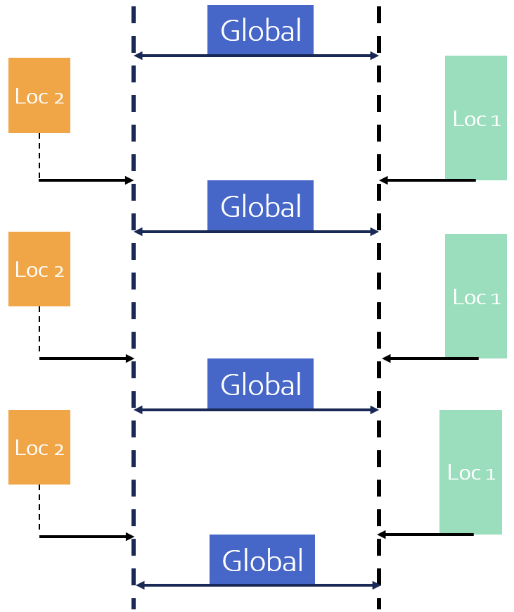
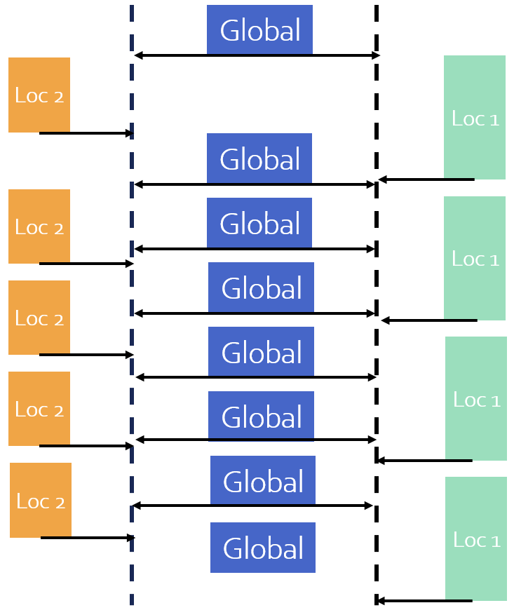
Figure 3(a) presents the time sequence of the classical synchronous approach, which alternates between global and parallel Fine calculations. Such an organization generates waiting and inactivity times on both sides, which seriously affects the performance. This phenomenon would be even amplified by bad load balancing, communication delays, or machine failures.

We establish an asynchronous parallel version of the Global/Local coupling to address these problems. The idea is to allow each processor to work at its own pace without waiting for the other processors, considering only the latest version of the available data. This technique leads to the time sequence of Figure 3(b) where processors only wait when they have no new data to process

(a) Synchronous iteration

(b) Asynchronous iteration

Figure 3: Time course of the Global/Local coupling in the case of two patches

Based on the figure3(b), the algorithm 2, presents an asynchronous version of the algorithm 1.

Initialization $\mathbf{p}_{\Gamma}=0$, $\omega$ sufficiently small

while $\|\mathbf{r}\|$ is too large do

       if Rank 0 is available and detects at least one new $\mathbf{q}^{s}$ then

             Resolution of the Global system (1) or (6), $\mathbf{u}^{G}_{\Gamma}=\mathbf{S}^{G^{-1}}(\mathbf{p}_{\Gamma}+\mathbf{b}^{G})$

             if $\Omega^{0}$ exists  then

                  Post-processing (3), $\mathbf{q}^{0}:=\boldsymbol{\lambda}^{0}=\mathbf{S}^{0}\mathbf{u}^{0,G}_{\Gamma}-\mathbf{b}^{0,G}$

             end if

            Global scatters $\mathbf{A}^{s^{T}}\mathbf{u}^{G}_{\Gamma}$ to subdmains $s>0$

            

       end if

      for $s>0$ do

             if Subdomain $s>0$ is available and detects new $(\mathbf{A}^{s^{T}}\mathbf{u}^{G})$ then

                   Patch receives $\mathbf{A}^{s^{T}}\mathbf{u}^{G}_{\Gamma}$

                   Fine solution (2), $\boldsymbol{\lambda}^{s,F}=\mathbf{S}^{s,F}\mathbf{J}^{s}\mathbf{A}^{s^{T}}\mathbf{u}^{G}_{\Gamma}-\mathbf{b}^{s,F}$

                   Patch sends of $\mathbf{q}^{s}:=\mathbf{J}^{s^{T}}\boldsymbol{\lambda}^{s,F}$ to the Global

             end if

            

       end for

      Global gathers all $\mathbf{q}^{s}$

       Global computes residual $\mathbf{r}=-\sum_{s}\mathbf{A}^{s}\mathbf{q}^{s}$

       Global updates $\mathbf{p}_{\Gamma}=\mathbf{p}_{\Gamma}+\omega\mathbf{r}$

end while

Algorithm 2 Asynchronous iterations

Note that the detection of the convergence of asynchronous iteration may require a specific, sometime complex, protocol [45, 41]. Since the Global/Local coupling always assembles the residual on the Global model, our stopping criterion can be the same as in the synchronous case, simply based on the norm of the residual.

3.2 Convergence proof of the asynchronous iteration

Proving the convergence of asynchronous iteration can be tedious. In our case, we have the advantage of the Global domain playing a special role such that it can be used to cadence the solver. Referring to Algorithm 2, we can consider that during the step from iteration $j$ to $j+1$, some patches provide new pieces of information in order to evaluate the residual, anyhow these pieces of information may be related to old configurations $p_{j-\sigma(s,j)}$ where $\sigma(s,j)\geqslant 0$ is a delay function. So that we can model the asynchronous iteration as:

$$\begin{cases}\begin{aligned} &\mathbf{u}^{G}_{\Gamma,j}=\mathbf{S}^{G^{-1}}(\mathbf{b}^{G}+{\mathbf{p}_{\Gamma}}_{j})\\ &\text{ If }s=0:\mathbf{q}^{0}_{j}=\mathbf{S}^{0}(\mathbf{A}^{0^{T}}\mathbf{u}^{G}_{\Gamma,j}-\mathbf{b}^{0,G})\\ &\text{ If }s>0:\mathbf{q}^{s}_{j}=\begin{cases}\mathbf{J}^{s^{T}}(\mathbf{S}^{s,F}\mathbf{J}^{s}\mathbf{A}^{s^{T}}\mathbf{u}^{G}_{\Gamma,j-\sigma(s,j)}-\mathbf{b}^{s,F})\text{ if updated }\\ \qquad\mathbf{q}^{s}_{j-1},\text{ if not updated }\\ \end{cases}\\ &\mathbf{r}_{j}=-\left(\mathbf{A}^{0}\mathbf{q}^{0}_{j}+\sum_{s>0}\mathbf{A}^{s}\mathbf{q}^{s}_{j}\right)\\ &{\mathbf{p}_{\Gamma}}_{j+1}={\mathbf{p}_{\Gamma}}_{j}+\omega\mathbf{r}_{j}\end{aligned}\end{cases}$$ (9)

For subdomains not updated, we set: $\sigma(s,j)=\sigma(s,j-1)+1$.

It is crucial to note that if it exists, subdomain $0$ always contributes to the evaluation of the residual because computing $\mathbf{q}^{0}_{j+1}$ is only a cheap postprocessing of the Global solution. In order to unify notations, we introduce $\sigma(0,j)=0$, $\forall j$, and then:

$${\mathbf{p}_{\Gamma}}_{j+1} ={\mathbf{p}_{\Gamma}}_{j}-\omega\sum_{s=0}^{N}\mathbf{A}^{s}\mathbf{J}^{s^{T}}(\mathbf{S}^{s,F}\mathbf{J}^{s}\mathbf{A}^{s^{T}}\mathbf{S}^{G^{-1}}({\mathbf{p}_{\Gamma}}_{j-\sigma(s,j)}+\mathbf{b}^{G})-\mathbf{b}^{s,F})$$ (10)

$$={\mathbf{p}_{\Gamma}}_{j}-\omega\left(\sum_{s=0}^{N}\mathbf{\hat{S}}^{s,F}\mathbf{S}^{G^{-1}}{\mathbf{p}_{\Gamma}}_{j-\sigma(s,j)}+\mathbf{\hat{b}}\right)$$

Note that this expression is valid only after all local patches have at least contributed once to the estimation of the residual.

In order to ensure that at some point all patches provide new information, we assume that:

$$\exists D\geqslant 0\text{ such that }\forall(s,j),\ \sigma(s,j)\leqslant D$$ (11)

For a given delay $0\leqslant k\leqslant D$, we write $\varpi(k,j)$ the set of subdomains $(s)$ such that $\sigma(s,j)=k$ so that the iteration can be rewritten as:

$${\mathbf{p}_{\Gamma}}_{j+1} ={\mathbf{p}_{\Gamma}}_{j}-\omega\left(\sum_{k=0}^{D}\left(\sum_{s\in\varpi(k,j)}\mathbf{\hat{S}}^{s,F}\right)\mathbf{S}^{G^{-1}}{\mathbf{p}_{\Gamma}}_{j-k}+\mathbf{\hat{b}}\right)$$ (12)

3.2.1 Tools for convergence study

The asynchronous Richardson iteration was the object of [11] in the case of a maximal delay of 2. In order to extend the method, we rely on the theory of paracontractions [16].

Let $(T_{m})$ be a finite family of paracontractions with a common fixed point $\hat{x}$ in some Hilbert space $E$. In other words:

• $\forall x\in E,\ \|T_{m}(x)-\hat{x}\|<\|x-\hat{x}\|$ or $T_{m}(x)=x$,

• $\forall m,\ T_{m}(\hat{x})=\hat{x}$.

Then a sequence of the form:

$$x_{j+1}=T_{m(j)}(x_{j})$$ (13)

converges to $\hat{x}$, assuming that all the paracontractions $(T_{m})$ are sufficiently frequently activated.

3.2.2 Analysis of Global/Local coupling

In order to make appear paracontraction, we assume a non-zero delay $D>0$, and we work in the “history space” obtained by concatenating the last $(D+1)$ values of ${\mathbf{p}_{\Gamma}}_{j}$.

We can rewrite the history at iteration $j+1$ as:

$$\begin{pmatrix}{\mathbf{p}_{\Gamma}}_{j+1}\\ {\mathbf{p}_{\Gamma}}_{j}\\ \vdots\\ {\mathbf{p}_{\Gamma}}_{j-D+1}\end{pmatrix}=\underset{\mathbf{B}_{j}}{\underbrace{\begin{pmatrix}\mathbf{I}-\omega\mathbf{X}_{j,0}&-\omega\mathbf{X}_{j,1}&\ldots&-\omega\mathbf{X}_{j,D}\\ \mathbf{I}&0&\ldots&0\\ 0&\mathbf{I}&0&\ldots\\ \ldots&0&\mathbf{I}&0\end{pmatrix}}}\begin{pmatrix}{\mathbf{p}_{\Gamma}}_{j}\\ {\mathbf{p}_{\Gamma}}_{j-1}\\ \vdots\\ {\mathbf{p}_{\Gamma}}_{j-D}\end{pmatrix}-\begin{pmatrix}\omega\tilde{\mathbf{b}}\\ 0\\ \vdots\\ 0\end{pmatrix}$$ (14)

$$\text{with }\mathbf{X}_{j,k}=\left(\sum_{s\in\varpi(k,j)}\mathbf{\hat{S}}^{s,F}\right)\mathbf{S}^{G^{-1}}$$

Since $\forall j,\ \sum_{k}\mathbf{X}_{j,k}\mathbf{\hat{p}}_{\Gamma}+\tilde{\mathbf{b}}=0$, the vector obtained by repeating the solution $\mathbf{\hat{p}}_{\Gamma}$ of (8) is a fixed point for the above iteration.

In order to prove the paracontracting nature of the iteration, it suffices to prove that any matrix $\mathbf{B}_{j}$ of (14) can be turned into contraction by correctly selecting the relaxation $\omega>0$. Since $\mathbf{B}_{j}$ is a block companion matrix, it seems natural to study its spectrum and prove that it can be bounded by 1.

The eigenvalues $(\lambda)$ of $\mathbf{B}_{j}$ are the roots of the polynomial:

$$\det\left((1-\lambda)\lambda^{D}\mathbf{I}-\omega\sum_{k=0}^{D}\lambda^{D-k}\mathbf{X}_{j,k}\right)=0$$ (15)

This is the determinant of a real momic matrix polynomial [25]. In order to benefit from the underlying symmetry, we can introduce the Cholesky factorization of $\mathbf{S}^{G}=\mathbf{L}\mathbf{L}^{T}$, left-multiply the polynomial by $\mathbf{L}^{-1}$ and right-multiply it by $\mathbf{L}$, the roots of (15) are also the root of the polynomial $P_{j,\omega}(\lambda)$:

$$P_{j,\omega}(\lambda) =\det\left((1-\lambda)\lambda^{D}\mathbf{I}-\omega\sum_{k=0}^{D}\lambda^{D-k}\mathbf{\hat{X}}_{j,k}\right)=0$$ (16)

where $\mathbf{\hat{X}}_{j,k}=\mathbf{L}^{-1}\mathbf{{X}}_{j,k}\mathbf{L}=\mathbf{L}^{-1}\left(\sum_{s\in\varpi(k,j)}\mathbf{\hat{S}}^{s,F}\right)\mathbf{L}^{-T}$.

Using the absolute continuity of the roots of a polynomial with respect to its coefficients (see [31, 48] for instance), we see that for a small enough $\omega$, the eigenvalues tend to concentrate around the roots of $P_{j,0}(\lambda)=\det((1-\lambda)\lambda^{D}\mathbf{I})$, that is to say around $0$ and $1$.

Let $\tilde{\lambda}_{j,\omega}$ be one of the roots of $P_{j,\omega}$, and $\varepsilon=\min\left(\sin\left(\frac{\pi}{3D}\right),\frac{1}{2}\right)$, we can find $\omega_{0}$ such that $\omega<\omega_{0}$ $\Rightarrow$ $|\tilde{\lambda}_{j,\omega}-\tilde{\lambda}_{j,0}|<\varepsilon$. At that point, the roots that tend to zero have all modulus less than $\varepsilon<1$, only the roots that tend to 1 could pose a problem. In what follows, $\tilde{\lambda}_{j,\omega}$ is such a root that tends to 1, we can bound its modulus and argument, see Figure 4.

Figure 4: Constraining roots near $1$

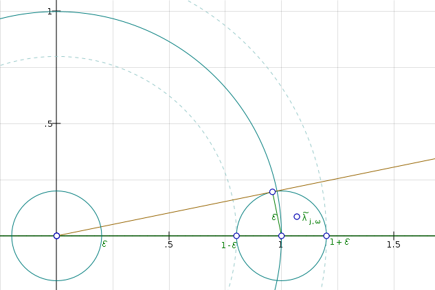
$|\tilde{\lambda}_{j,\omega}-1|<\varepsilon$ implies that:

$$1-\varepsilon<|\tilde{\lambda}_{j,\omega}|<1+\varepsilon$$ (17)

$$|\sin(\arg(\tilde{\lambda}_{j,\omega}))|<\varepsilon$$

For $\varepsilon=\sin{\frac{\pi}{3D}}$ and $0\leqslant k\leqslant D$, we have bounds on the modulus and on the reel part (symbol $\Re$):

$$(1-\varepsilon)^{D} <|\tilde{\lambda}_{j,\omega}|^{k}<(1+\varepsilon)^{D}$$ (18)

$$\Re(\tilde{\lambda}^{k}_{j,\omega}) =|\tilde{\lambda}_{j,\omega}|^{k}\cos(k\arg(\tilde{\lambda}_{j,\omega}))>\frac{(1-\varepsilon)^{D}}{2}$$

Let $\mathbf{\tilde{v}}_{j,\omega}$ be an eigenvector of the matrix polynomial associated with $\tilde{\lambda}_{j,\omega}$:

$$(1-\tilde{\lambda}_{j,\omega})\tilde{\lambda}_{j,\omega}^{D}\mathbf{\tilde{v}}_{j,\omega}-\omega\sum_{k=0}^{D}\tilde{\lambda}_{j,\omega}^{D-k}\mathbf{\hat{X}}_{j,k}\mathbf{\tilde{v}}_{j,\omega} =0$$ (19)

We can left-multiply the expression by the Hermitian transpose $\mathbf{\tilde{v}}_{j,\omega}^{H}$:

$$(1-\tilde{\lambda}_{j,\omega})\tilde{\lambda}_{j,\omega}^{D}\mathbf{\tilde{v}}^{H}_{j,\omega}\mathbf{\tilde{v}}_{j,\omega}-\omega\sum_{k=0}^{D}\tilde{\lambda}_{j,\omega}^{D-k}\mathbf{\tilde{v}}^{H}_{j,\omega}\mathbf{\hat{X}}_{j,k}\mathbf{\tilde{v}}_{j,\omega} =0$$ (20)

To simplify, $\mathbf{\tilde{v}}_{j,\omega}$ can be chosen of unit Euclidean norm. For $\omega<\omega_{0}$ we have $\tilde{\lambda}_{j,\omega}\neq 0$, and then:

$$\tilde{\lambda}_{j,\omega} =1-\omega\sum_{k=0}^{D}\frac{\|\mathbf{\tilde{v}}_{j,\omega}\|^{2}_{\mathbf{\hat{X}}_{j,k}}}{\tilde{\lambda}_{j,\omega}^{k}}$$ (21)

$$|\tilde{\lambda}_{j,\omega}|^{2} =1-2\omega\sum_{k=0}^{D}\frac{\Re(\tilde{\lambda}_{j,\omega}^{k})\|\mathbf{\tilde{v}}\|^{2}_{\mathbf{\hat{X}}_{j,k}}}{|\tilde{\lambda}_{j,\omega}|^{2k}}+\omega^{2}\left|\sum_{k=0}^{D}\frac{\|\mathbf{\tilde{v}}\|^{2}_{\mathbf{\hat{X}}_{j,k}}}{\tilde{\lambda}_{j,\omega}^{k}}\right|^{2}$$

Using (18), we have:

$$|\tilde{\lambda}_{j,\omega}|^{2} <1-\omega\frac{\left(\sum_{k=0}^{D}\|\mathbf{\tilde{v}}\|^{2}_{\mathbf{\hat{X}}_{j,k}}\right)}{(1+\varepsilon)^{D}}+\omega^{2}\frac{\left(\sum_{k=0}^{D}\|\mathbf{\tilde{v}}\|^{2}_{\mathbf{\hat{X}}_{j,k}}\right)^{2}}{(1-\varepsilon)^{2D}}$$ (22)

The sum of norms is simplified because each subdomain appears only once:

$$\sum_{k=0}^{D}\|\mathbf{\tilde{v}}\|^{2}_{\mathbf{\hat{X}}_{j,k}} =\sum_{k=0}^{D}\mathbf{\tilde{v}}_{j,\omega}^{H}\mathbf{\hat{X}}_{j,k}\mathbf{\tilde{v}}_{j,\omega}=\mathbf{\tilde{v}}_{j,\omega}^{H}\mathbf{L}^{-1}\left(\sum_{k=0}^{D}\sum_{s\in\varpi(k,j)}\mathbf{\hat{S}}^{s,F}\right)\mathbf{L}^{-T}\mathbf{\tilde{v}}_{j,\omega}$$ (23)

$$=\mathbf{\tilde{v}}_{j,\omega}^{H}\mathbf{L}^{-1}\left(\sum_{s=0}^{N}\mathbf{\hat{S}}^{s,F}\right)\mathbf{L}^{-T}\mathbf{\tilde{v}}_{j,\omega}$$

Since $\mathbf{\tilde{v}}_{j,\omega}$ is of unit Euclidean norm, the term above can directly be bounded by the extremal eigenvalues of $\mathbf{L}^{-1}\left(\sum_{s=0}^{N}\mathbf{\hat{S}}^{s,F}\right)\mathbf{L}^{-T}$ which coincide to the generalized eigenvalues of the pair of matrices $(\sum_{s=0}^{N}\mathbf{\hat{S}}^{s,F},\mathbf{S}^{G})$:

$$\alpha_{\min} \leqslant\sum_{k=0}^{D}\|\mathbf{\tilde{v}}\|^{2}_{\mathbf{\hat{X}}_{j,k}}\leqslant\alpha_{\max}$$ (24)

$$\text{where the }(\alpha)\text{ solve } \det\left(\left(\sum_{s=0}^{N}\mathbf{\hat{S}}^{s,F}\right)+\alpha\mathbf{S}^{G}\right)=0$$

We thus obtain the upper bound:

$$|\tilde{\lambda}_{j,\omega}|^{2} \leqslant 1-\omega\frac{\alpha_{\min}}{(1+\varepsilon)^{D}}+\omega^{2}\frac{\alpha_{\max}^{2}}{(1-\varepsilon)^{2D}},\qquad\forall 0<\omega<\omega_{0}$$ (25)

This is a bound of the form $|\tilde{\lambda}_{j,\omega}|^{2}\leqslant 1-A\omega+B\omega^{2}$ (with $0<A<B$) which is a second degree polynomial in $\omega$, and which is less than 1 for $0<\omega<A/B$. As a consequence:

$$|\tilde{\lambda}_{j,\omega}|<1\text{ for }0<\omega<\omega_{\mathrm{async}}=\min\left(\omega_{0},\frac{(1-\varepsilon)^{D}\alpha_{\min}}{(1+\varepsilon)^{2D}\,\alpha_{\max}^{2}}\right)$$ (26)

This is probably an extremely crude bound, but it has the advantage to only depend on $D$ and not on the configuration of the iteration (index $j$). Thus, such a relaxation makes any $\mathbf{B}_{j}$ a paracontraction, and it makes the asynchronous iteration converge.

Remark 1.

For the synchronous iteration, the bound can be derived from (15) with $D=0$, it is $0<\omega<\omega_{\mathrm{sync}}=\frac{2}{\alpha_{\max}}$. Note that $\omega_{\mathrm{sync}}>\omega_{\mathrm{async}}$.

3.3 Implementation details

Several approaches are available in the literature to implement asynchronous model. In [42, 40], an efficient library is proposed for asynchronous domain decomposition solvers, based on classical non-blocking two-sided communications. In [59, 24] the use of one-sided communications, also known as MPI-RDMA (Remote Direct Memory Access), is considered. The one-sided communication is meant to reduce management overhead. Note that the performance of the RDMA strongly depends on the MPI implementation and the network hardware.

The basic idea is that each rank exposes a so-called window of its local memory and grants other ranks write or read access. Ranks, in this case, are no longer identified as sender or receiver but as origin rank who initiates the operation and target rank. The latter does not participate in the data exchange.

The RMA-MPI workflow is based on the following five steps:

1. Allocation of the window (local memory buffer accessible from other ranks).

2. Epoch opening: beginning of the period when the window is open the other ranks.

3. Data accessing: Each origin rank can access the target ranks’ window to Put (write data) or to Get (read data). See Figure 5(a) where Processor 0 puts a data Y in Processor 1 window and Figure 5(b) where Processor 1 gets a data Y from Processor 0 window.

4. Epoch closing: the target rank which closes the windows ensures that all accesses are completed (local synchronization). At this point, the target rank can read and process the data put by other ranks.

5. Window freeing: liberation of the memory buffer.

(a) Put

(b) Get

Figure 5: One-sided communication concepts [18]

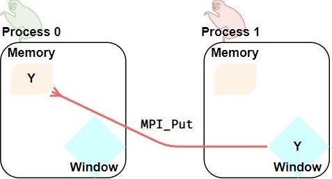
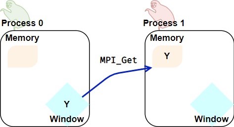
To secure the data access in a window, one may consider two ways:

Active synchronization

consists in performing a collective blocking call on both the target and origin using the MPI.Fence() command at the beginning and at the end of the epoch to synchronize the data.

Passive synchronization

emulates shared memory. The target processor is not involved in the management of the data, full asynchronous communication is possible. MPI.Lock(Target rank) opens an epoch and allows the origin processor to access securely the target’s window. The epoch is then closed by MPI.Unlock(Target rank). To ensure the completion of an operation within an epoch, one can use MPI.Flush(Target rank)

Algorithm 3 proposes an RDMA implementation of the asynchronous version of the Global/Local coupling algorithm 2 with passive synchronization. The principle is to have the subdomains compute whenever they idle and a new piece of information becomes available: a new interface Dirichlet condition for the fine patches, any new interface nodal reaction for the global model.

Window creation + Initialization $\mathbf{p}_{\Gamma}=0$, $\omega$ sufficiently small

MPI.Lock(target) (For all the window by specifying the specific target of each one) while $\|\mathbf{r}\|$ is too large do

       if Rank 0 is available and detects at least one new $\mathbf{q}^{s}$ then

             Resolution of the Global system (1) or (6), $\mathbf{u}^{G}_{\Gamma}=\mathbf{S}^{G^{-1}}(\mathbf{p}_{\Gamma}+\mathbf{b}^{G})$

             if $\Omega^{0}$ exists  then

                  Post-processing (3), $\mathbf{q}^{0}:=\boldsymbol{\lambda}^{0}=\mathbf{S}^{0}\mathbf{u}^{0,G}_{\Gamma}-\mathbf{b}^{0,G}$

             end if

            Put $\mathbf{A}^{s^{T}}\mathbf{u}^{G}_{\Gamma}$ in subdmains $s>0$ windows + Flush(subdomains s window)

            

       end if

      for $s>0$ do

             if Subdomain $s>0$ is available and detects new $(\mathbf{A}^{s^{T}}\mathbf{u}^{G})$ then

                   Fine solution (2), $\boldsymbol{\lambda}^{s,F}=\mathbf{S}^{s,F}\mathbf{J}^{s}\mathbf{A}^{s^{T}}\mathbf{u}^{G}_{\Gamma}-\mathbf{b}^{s,F}$

                   Put of $\mathbf{q}^{s}:=\mathbf{J}^{s^{T}}\boldsymbol{\lambda}^{s,F}$ to the rank 0 window + Flush(0)

                  

             end if

            

       end for

      Global computes residual $\mathbf{r}=-\sum_{s}\mathbf{A}^{s}\mathbf{q}^{s}$

       Global updates $\mathbf{p}_{\Gamma}=\mathbf{p}_{\Gamma}+\omega\mathbf{r}$

end while

MPI.UnLock(target) (For all the window by specifying the specific target of each one)

Algorithm 3 Asynchronous iterations using RDMA

Remark 2.

An RDMA implementation of the synchronous coupling in algorithm 1 is proposed in Algorithm 4, it makes use of active synchronization with MPI.Fence().

Window creation + Initialization $\mathbf{p}_{\Gamma}=0$, $\omega$ sufficiently small

while $\|\mathbf{r}\|$ is too large do

       MPI.Fence()(For the global displacement window)

       if rank == 0 then

             Resolution of the Global system (1) or (6), $\mathbf{u}^{G}_{\Gamma}=\mathbf{S}^{G^{-1}}(\mathbf{p}_{\Gamma}+\mathbf{b}^{G})$

             if $\Omega^{0}$ exists  then

                  Post-processing (3), $\mathbf{q}^{0}:=\boldsymbol{\lambda}^{0}=\mathbf{S}^{0}\mathbf{u}^{0,G}_{\Gamma}-\mathbf{b}^{0,G}$

             end if

            Put $\mathbf{A}^{s^{T}}\mathbf{u}^{G}_{\Gamma}$ in subdmains $s>0$ windows ;

       end if

      MPI.Fence()(For the global displacement window)

       MPI.Fence()(For the local nodal reaction)

       if rank != 0 then

             Fine solution (2), $\boldsymbol{\lambda}^{s,F}=\mathbf{S}^{s,F}\mathbf{J}^{s}\mathbf{A}^{s^{T}}\mathbf{u}^{G}_{\Gamma}-\mathbf{b}^{s,F}$

             Patch Put $\mathbf{q}^{s}:=\mathbf{J}^{s^{T}}\boldsymbol{\lambda}^{s,F}$ in the rank 0 window

       end if

      MPI.Fence()(For the local nodal reaction)

       MPI.Fence()(For the convergence detection window)

       if rank == 0 then

             Global computes residual $\mathbf{r}=-\sum_{s}\mathbf{A}^{s}\mathbf{q}^{s}$

             Global updates $\mathbf{p}_{\Gamma}=\mathbf{p}_{\Gamma}+\omega\mathbf{r}$

       end if

      MPI.Fence()(For the convergence detection window)

      

end while

Window free

Algorithm 4 Synchronous stationary iterations using RDMA

4 Applications

To illustrate the theory presented above, we consider two kind of equations. First the Poisson equation, which models thermal problems:

$$\text{Find }u :\Omega\subset\mathbb{R}^{d}\to\mathbb{R}$$ (27)

$$\operatorname{div}(a\operatorname{grad}(u)) =1\text{ in }\Omega$$

$$u =0\text{ on }\partial_{d}\Omega$$

$$\frac{\partial u}{\partial n} =0\text{ on }\partial\Omega\setminus\partial_{d}\Omega$$

for simplicity, we used unit source term and homogeneous boundary conditions. In some cases a contrast of conductivity coefficient $a$ is used.

Second, the linear elasticity equation:

$$\text{Find }u :\Omega\subset\mathbb{R}^{d}\to\mathbb{R}^{d}$$ (28)

$$\operatorname{div}(\sigma)+f =0\text{ in }\Omega$$

$$u =0\text{ on }\partial_{d}\Omega$$

$$\sigma\cdot n =0\text{ on }\partial\Omega\setminus\partial_{d}\Omega$$

$$\sigma =\frac{E}{1+\nu}\left(\varepsilon(u)+\frac{\nu}{1-2\nu}\operatorname{tr}(\varepsilon(u))I\right)$$

$$\varepsilon(u) =\frac{1}{2}(\nabla u+(\nabla u)^{T})$$

$E$ is Young’s modulus, and $\nu=0.3$ is Poisson’s coefficient. In some cases, a contrast of Young’s modulus is used. The value of the source term f varies with the study cases.

We propose to assess the asynchronous Global/Local coupling on two academic examples: the simple 2D case of Figures 1(a) and 1(b), and a more challenging 3D case involving many patches. In order to evaluate the performance we compare the following approaches:

• non-relaxed synchronous iteration ($\omega=1$),

• Aitken-accelerated (synchronous) iteration,

• non-relaxed asynchronous iteration ($\omega=1$),

• asynchronous iteration with optimized relaxation.

Aitken’s acceleration can be viewed as an efficient way to find a good dynamic relaxation. The optimized relaxation coefficient for the asynchronous iteration is obtained by trial-and-error.

Our Ethernet network does not support RDMA communication by default. It generates implicit synchronizations when we use MPI.Lock() and MPI.Unlock() commands to check if new data is available in the target processor. In order to achieve the best possible time, we used a computational sequence slightly different than Figure 3(b): processors always compute with the available data without checking for their novelty (thus possibly redoing the same calculus several times but never triggering unwanted sync).

Our code is realized in Python with mpi4py module [14]. It uses several other tools and software like GMSH [23] to generate the geometries and meshes of the studied cases. For the finite element approximation, we use the GetFEM library [51].

The study was carried out with the cluster of the LMPS simulation center using several workstations with an Ethernet network. These machines are quite heterogeneous with 4 different generation of CPUs :(Intel(R) Xeon(R) CPU E5-1660 v3 (Haswell) @ 3.00GHz, Intel(R) Xeon(R) CPU E5-2630 v4 (Broadwell) @ 2.20GHz, Intel(R) Xeon(R) Silver 4116 CPU (Skylake) @ 2.10GHz, Intel(R) Xeon(R) W-2255 CPU (Cascade Lake) @ 3.70GHz.

4.1 Simple 2D test-case

To begin with the illustrations, we use the test-case of Figures 1(a) and 1(b) where the patches only introduce geometric alterations. The patches and the global model are treated on three different CPUs.

As shown in Table 1, the problem is of very small dimension, and the patches are well-balanced, which is in favor of synchronous algorithms.

Problem	Global	$1^{st}$ zone of interest	$2^{nd}$ zone of interest
#nodes	701	381	379

Table 1: Size of the domains or the 2D test case.

Tables 2 and 3 present the performance in terms of time and number of iterations. In the asynchronous cases, the number of local solves may differ from the number of iterations, so the range of the number of local solves is also indicated. For these small cases, Aitken remains unbeatable. We observe the interest of finding a good relaxation for the asynchronous iteration to perform better than the non-relaxed synchronous iteration.

Variant	Sync.
$\omega=1$	Sync.
Aitken	Async.
$\omega=1$	Async.
$\omega_{\mathrm{opt}}$
Time (s)	0.22	0.12	0.3	0.19
#iter. glob.	23	12	45	29
#loc. sol. [min, max]	$\cdot$	$\cdot$	[96,97]	[64,65]

Table 2: 2D test-case: performance for thermal problem.

Variant	Sync.
$\omega=1$	Sync.
Aitken	Async.
$\omega=1$	Async.
$\omega_{\mathrm{opt}}$
Time (s)	0.67	0.3	0.6	0.52
#iter. glob.	43	16	53	48
#loc. sol. [min, max]	$\cdot$	$\cdot$	[112,119]	[100,107]

Table 3: 2D test-case: performance for the elasticity problem.

What is more interesting to observe is the large amount of computation that can be done by the asynchronous solver thanks to the removal of waiting time.

4.2 Weak scalability 3D test-case

Weak scalability tests aim at proving the ability of the method to solve large problems in reasonable time.

In order to be able to generate test-cases with many patches, we created a cuboid geometry made out of $n^{3}$ ($n=2..7$) cube patches. As classically done for weak scalability assessment of domain decomposition methods, the size of the domain increases with the number of subdomains. Note that the whole domain is covered with patches ($\Omega^{0}=\emptyset$). The Global model is homogeneous, whereas the Local models contain one softer spherical inclusion, see Figures 6(a) and 6(b). One side of the Global model is submitted to Dirichlet conditions.

In the case of thermal problems, the inclusions have a diffusion coefficient 10 times lower than the rest of the domain, whereas in the elasticity case the Young’s modulus in the inclusions is 100 times lower than in the rest of the domain.

(a) Global model

(b) Reference model

Figure 6: Weak scalability test-case: $2\times 2\times 2$ subdomains

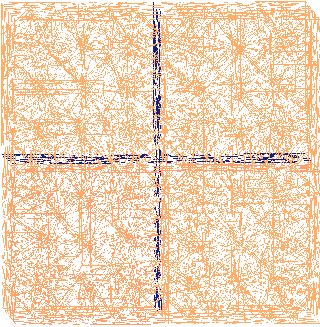
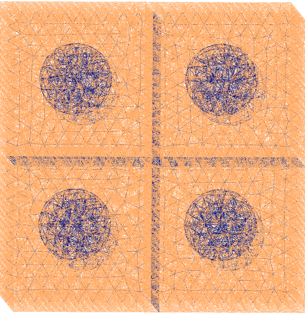
Even if their meshes are not identical, the patches are well-balanced in terms of degrees of freedom and numerical complexity (since the problem is linear). Of course, the Global model grows along the study, from 8 times smaller than one patch to 3.7 times larger. This is a strong limitation of the method in comparison with classical domain decomposition methods were the coarse problem’s growth is much more moderate. Table 4 sums up the number of nodes for each case.

#subdomains	8	27	64	125	216	343
#nodes of glob. problem	233	667	1449	2681	4465	6903
#nodes of per loc. problem (= 1 subdomain)	1858	1858	1858	1858	1858	1858

Table 4: Number of nodes in the meshes for the weak scalability study.

Figure 7: Time performance in the weak scalability study for linear thermal problem

Figure 8: Time performance in the weak scalability study for linear elasticity problem

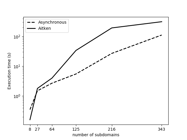
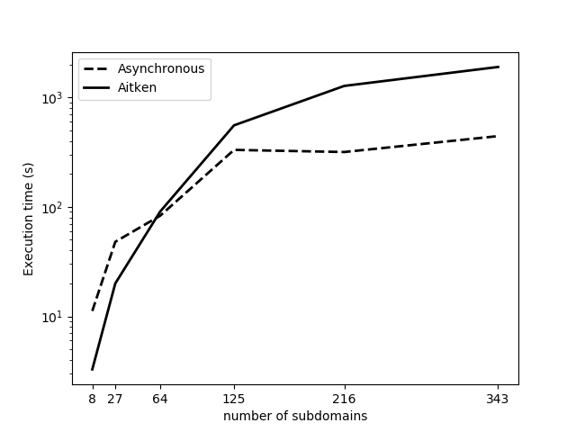
Figures 8 and 7 compare the performance in wall-clock time of the relaxed asynchronous iteration (with hand-tuned relaxation) and the synchronous iteration with Aitken’s dynamic relaxation. We observe the good performance of the asynchronous version despite the good load-balancing.

For the small test-cases (8 and 27 subdomains), the size of the global problem is negligible compared to the size of the local problems. This means that the sequential phase of the synchronous coupling is realized very quickly and this leads to the Aitken accelerator being faster than the asynchronous solver. However, for 64 subdomains and more, this step becomes heavier and takes more synchronous time. For the asynchronous method, the Global solve is realized simultaneously with the local solves. Thus, the execution time increases very slightly from one case to another and remains 2 to 3 times less than for Aitken.

#patches	8	27	64	125	216	343
Aitken #iter.	11	13	12	11	11	11
Async. #iter. glob.	255	256	87	65	69	71
Async. #loc. sol. [min, max]	[32,39]	[43,74]	[49,153]	[84,207]	[276,694]	[407,2902]

Table 5: Weak scalability: Number of iterations in the thermal case.

#patches	8	27	64	125	216	343
Aitken #iter.	22	21	25	25	26	29
Async. #iter. glob.	2065	1349	372	296	295	209
Async. #loc. sol. [min, max]	[78,240]	[102,237]	[128,475]	[157,517]	[147,514]	[175,407]

Table 6: Weak scalability: Number of iterations in the elasticity case.

Tables 5 and  6 gather the number of iterations for each case. In the asynchronous case, the number of iterations (or Global solves) is given as well as the minimum and maximum numbers of patches’ solve. We see that the number of iterations barely varies in the synchronous experiments (in particular for the thermal problem) for all studied cases.

For the asynchronous solver, it can be seen that in the 8 and 27 patches cases where the global problem is very small, many more solves are performed by the global domain than by the local patches. Because of the non-waiting asynchronous model the global problem repeats several times the same calculation without having new information from the locals, however when the size of this problem increases (more than 64 subdomains), we begin to see that the patches make more repeated iterations while waiting for the update of the global problem which performs only a few iterations.

Note the performance achieved in the elasticity case (2 times faster) despite the tremendous number of iterations (7 times more).

4.3 Poor load balancing

We wish to evaluate the influence of a significant disequilibrium in the number of nodes to be handled by processors. We start from a geometry formed with a $16\times 4\times 4$ repetition of cubes with spherical inclusion (this time 1000 times stiffer than the rest of the domain), see Figure 9.

Figure 9: Fine representation with unbalanced subdomains

Each Fine subdomain has a randomly chosen number of nodes compared to the other subdomains, allowing to have very refined subdomains and others slightly refined. Table 7 summarizes the number of nodes for the global problem and the smallest and largest number of nodes among the 256 Fine subdomains. We can see that the most refined subdomain is ten times larger than the least refined.

	Global	Smallest local	Biggest local
#nodes	5490	534	4698

Table 7: Mesh

Variant	Sync.
Aitken	Async.
$\omega_{\mathrm{opt}}$
Time (s)	881.55	79.44
#iter. glob.	36	506
#loc. sol. [min, max]	$\cdot$	[348, 6788]

Table 8: Poor load balancing case: Iterations & Time (thermal problem)

Variant	Sync.
Aitken	Async.
$\omega_{\mathrm{opt}}$
Time (s)	3509.6	1904.34
#iter. glob.	113	2354
#loc. sol. [min, max]	$\cdot$	[818, 2951]

Table 9: Poor load balancing case: Iterations & Time (linear elasticity problem)

This case study has been performed using 257 processors, one for the global problem and one processor for each one of the 256 local problems. Table 8 and 9 show the computation time and the number of iterations.

We see that even if the number of iterations can be very large in the asynchronous case, the CPU time is much reduced: 10 times in the thermal case and 2 times for the elasticity case. Again, this highlights the prohibitive cost of synchronization.

5 Conclusion

An asynchronous version of the non-intrusive global/local computation method has been presented for linear elliptic problems, starting from the new interpretation of the method as a right-preconditioned primal domain decomposition method. A proof of convergence has been established for the discretized system using paracontractions techniques. An implementation with MPI RDMA parallelization has been set. The coupling has been tested on linear thermal and elasticity problems involving up to hundreds of patches. The performance in terms of computation time is convincing: the asynchronous method (with hand tuned relaxation) is faster than the synchronous solver with Aitken’s dynamic relaxation on a cluster of heterogeneous machines.

Future work should focus on finding an efficient estimation of the optimal relaxation for the asynchronous iteration.

References

- [1] Olivier Allix and Pierre Gosselet. Non intrusive global/local coupling techniques in solid mechanics: An introduction to different coupling strategies and acceleration techniques. In L. De Lorenzis and A. Düster, editors, Modeling in Engineering Using Innovative Numerical Methods for Solids and Fluids, volume 599 of CISM International Centre for Mechanical Sciences – Courses and Lectures, pages 203–220. Springer Nature Switzerland AG, February 2020.
- [2] Gerard M. Baudet. Asynchronous iterative methods for multiprocessors. Journal of the Association for Computing Machinery, 25(2), 1978.
- [3] Omar Bettinotti, Olivier Allix, and Benoît Malherbe. A coupling strategy for adaptive local refinement in space and time with a fixed global model in explicit dynamics. Computational Mechanics, pages 1–14, 2013.
- [4] Omar Bettinotti, Olivier Allix, Umberto Perego, Victor Oncea, and Benoît Malherbe. A fast weakly intrusive multiscale method in explicit dynamics. International Journal for Numerical Methods in Engineering, 100(8):577–595, 2014.
- [5] Omar Bettinotti, Olivier Allix, Umberto Perego, Victor Oncea, and Benoît Malherbe. Simulation of delamination under impact using a global local method in explicit dynamics. Finite Elements in Analysis and Design, 125:1–13, 2017.
- [6] Maxime Blanchard, Olivier Allix, Pierre Gosselet, and Geoffrey Desmeure. Space/time global/local noninvasive coupling strategy: Application to viscoplastic structures. Finite Elements in Analysis and Design, 156:1–12, April 2019.
- [7] José C.Garay, Frédéric Magoulès, and Daniel B.Szyld. Synchronous and asynchronous optimized schwarz methods for poisson’s equation in rectangular domains. Electron. Trans. Numer. Anal., 55:744–791, 2022.
- [8] D. Chazan and W. Miranker. Chaotic relaxation. Linear Algebra and Its Application, 2:199–222, 1969.
- [9] M. Chevreuil, A. Nouy, and E. Safatly. A multiscale method with patch for the solution of stochastic partial differential equations with localized uncertainties. Computer Methods in Applied Mechanics and Engineering, 255(0):255–274, 2013.
- [10] Edmond Chow, Andreas Frommer, and Daniel B.Szyld. Asynchronous richardson iterations: theory and practice. Numerical algorithms, 87:1635–1651, 2021.
- [11] Edmond Chow, Andreas Frommer, and Daniel B.Szyld. AsynchronousRichardson iterations: theory and practice. Numerical Algorithms, 87(4):1635–1651, 2021.
- [12] N. G. Cormier, B. S. Smallwood, G. B. Sinclair, and G. Meda. Aggressive submodelling of stress concentrations. International Journal for Numerical Methods in Engineering, 46(6):889–909, 1999.
- [13] Philippe Cresta, Olivier Allix, Christian Rey, and Stéphane Guinard. Nonlinear localization strategies for domain decomposition methods: application to post-buckling analyses. Computer Methods in Applied Mechanics and Engineering, 196(8):1436–1446, 2007.
- [14] Lisandro Dalcin and Yao-Lung L.Fang. mpi4py: Status update after 12 years of development,. Computing in Science & Engineering, 23(4):47–54, 2021.
- [15] Mickaël Duval, Jean-Charles Passieux, Michel Salaün, and Stéphane Guinard. Non-intrusive coupling: recent advances and scalable nonlinear domain decomposition. Archives of Computational Methods in Engineering, pages 1–22, 2014.
- [16] L. Eisner, I. Koltracht, and M. Neumann. Convergence of sequential and asynchronous nonlinear paracontractions. Numerische Mathematik, 62:305–319, 1992.
- [17] Mouhamed Nabih El Tarazi. Some convergence results for asynchronous algorithms. Numerische Mathematik, 39:325–340, 1982.
- [18] ENCC and Sweden. Intermediate mpi : One-sided communication concepts. https://enccs.github.io/intermediate-mpi/one-sided-concepts, 2020.
- [19] Andreas Frommer and Daniel B.Szyld. On asynchronous iterations. Journal of Computational and Applied Mathematics,, 123:201–216, 2000.
- [20] Guillaume Gbikpi-Benissan and Frédéric Magoulès. Asynchronous substructuring method with alternating local and global iterations. Journal of Computational and Applied Mathematics, 393:116–133, 2021.
- [21] Guillaume Gbikpi-Benissan and Frédéric Magoulès. Resilient asynchronous primal schur method. Applications of Mathematics, 2022.
- [22] Lionel Gendre, Olivier Allix, Pierre Gosselet, and François Comte. Non-intrusive and exact global/local techniques for structural problems with local plasticity. Computational Mechanics, 44(2):233–245, 2009.
- [23] Christophe Geuzaine and Jean-François Remacle. Gmsh : a three-dimensional nite element mesh generator with built-in pre- and post-processing facilities,. International Journal for Numerical Methods in Engineering, 79(11):1309–1331, 2009.
- [24] Christian Glusa, Erik Boman, Edmond Chow, Siva Rajamanickam, and Daniel B.Szyld. Sacalable asynchronous domain decomposition solvers. SIAM Journal on Scientific Computing, 42(6):384–409, 2020.
- [25] I. Gohberg, P. Lancaster, and L. Rodman. Matrix Polynomials. Society for Industrial and Applied Mathematics, 2009.
- [26] Pierre Gosselet, Maxime Blanchard, Olivier Allix, and Guillaume Guguin. Non-invasive global-local coupling as a Schwarz domain decomposition method: acceleration and generalization. Advanced Modeling and Simulation in Engineering Sciences, 5(4), 2018.
- [27] Pierre Gosselet and Christian Rey. Non-overlapping domain decomposition methods in structural mechanics. Archives of computational methods in engineering, 13(4):515–572, 2007.
- [28] Guillaume Guguin, Olivier Allix, Pierre Gosselet, and Stéphane Guinard. On the computation of plate assemblies using realistic 3d joint model: a non-intrusive approach. Advanced Modeling and Simulation in Engineering Sciences, 3(16), 2016.
- [29] F. Hecht, A. Lozinski, and O. Pironneau. Numerical zoom and the Schwarz algorithm. In Proceedings of the 18th conference on domain decomposition methods, pages 63–73, 2009.
- [30] J. Hinojosa, O. Allix, P.A. Guidault, and P. Cresta. Domain decomposition methods with nonlinear localization for the buckling and post-buckling analyses of large structures. Advances in Engineering Software, 70:13–24, 2014.
- [31] Kenichi Hirose. Continuity of the roots of a polynomial. The American Mathematical Monthly, 127(4):359–363, 2020.
- [32] C. C. Jara-Almonte and C. E. Knight. The specified boundary stiffness/force SBSF method for finite element subregion analysis. International Journal for Numerical Methods in Engineering, 26(7):1567–1578, 1988.
- [33] FS Kelley. Mesh requirements for the analysis of a stress concentration by the specified boundary displacement method. In Proceedings of the Second International Computers in Engineering Conference, ASME, pages 39–42, 1982.
- [34] David E Keyes. Aerodynamic applications of Newton-Krylov-Schwarz solvers. In Fourteenth International Conference on Numerical Methods in Fluid Dynamics, pages 1–20. Springer, 1995.
- [35] Axel Klawonn and Olof Widlund. Feti and neumann-neumann iterative substructuring methods: Connections and new results. Communications on Pure and Applied Mathematics, 54(1):57–90, 2001.
- [36] Pierre Ladevèze, Olivier Loiseau, and David Dureisseix. A micro-macro and parallel computational strategy for highly heterogeneous structures. International Journal for Numerical Methods in Engineering, 52(1-2):121–138, 2001.
- [37] P. Le Tallec, Y. H. De Roeck, and M. Vidrascu. Domain decomposition methods for large linearly elliptic three-dimensional problems. Journal of Computational and Applied Mathematics, 34(1):93, 1991.
- [38] Frédéric Magoules and Cédric Venet. Asynchronous iterative sub-structuring methods. Mathematics and Computers in Simulation, 145:34–49, 2018.
- [39] Frédéric Magoulès, Daniel B.Szyld, and Cédric Venet. Asynchronous optimized schwarz methods with and without overlap. Numerische Mathematik, 137:199–227, 2017.
- [40] Frédéric Magoulès and Guillaume Gbikpi-Benissan. Jack: An asynchronous communication kernel library for iterative algorithms. The Journal of Supercomputing, 73(8):3468–3487, 2017.
- [41] Frédéric Magoulès and Guillaume Gbikpi-Benissan. Distributed convergence detection based on global residual error under asynchronous iterations,. IEEE transactions on parallel and distributed systems, 29, 2018.
- [42] Frédéric Magoulès and Guillaume Gbikpi-Benissan. Jack2: An mpi-based communication library with non-blocking synchronization for asynchronous iterations. Advances in Engineering Software, 119:116–133, 2018.
- [43] Jan Mandel. Balancing domain decomposition. Communications in Numerical Methods in Engineering, 9(3):233, 1993.
- [44] Jean-Claude Miellou. Algorithmes de relaxation chaotiques à retard. ESAIM Mathematical modelling and numerical analysis, 9:55–82, 1975.
- [45] Jean-Claude Miellou, Pierre Spiteri, and Didier El Baz. A new stopping criterion for linear perturbed asynchronous iterations,. Journal of Computational and Applied Mathematics, 219:471–483, 2008.
- [46] Camille Negrello, Pierre Gosselet, Christian Rey, and Julien Pebrel. Substructured formulations of nonlinear structure problems — influence of the interface condition. International Journal for Numerical Methods in Engineering, 107(13):1083–1105, 2016.
- [47] Anthony Nouy and Florent Pled. A multiscale method for semi-linear elliptic equations with localized uncertainties and non-linearities. ESAIM: Mathematical Modelling and Numerical Analysis, 2018. 39 pages.
- [48] Adam Parusinski and Armin Rainer. Optimal regularity of roots of polynomials. working paper or preprint, March 2016.
- [49] Dimitri P.Bertsekas. Distributed asynchronous computation of fixed points. Mathematical Programming, 27(599):107 – 120, 1983.
- [50] Jonathan B Ransom, Susan L McCleary, Mohammad A Aminpour, and Norman F Knight Jr. Computational methods for global/local analysis. NASA STI/Recon Technical Report N, 92:33104, 1992.
- [51] Yves Renard and Konstantinos Poulios. Getfem: Automated fe modeling of multiphysics problems based on a generic weak form language,. Advances in Engineering Software, 47:1–31, 2021.
- [52] Nicole Spillane and Daniel J. Rixen. Automatic spectral coarse spaces for robust FETI and BDD algorithms. Internat. J. Num. Meth. Engin., 95(11):953–990, 2013.
- [53] Pierre Spiteri. Parallel asynchronous algorithms: A survey. Advances in Engineering Software, 149:102896, 2020.
- [54] Pierre Spiteri, Jean-Claude Miellou, and Didier El Baz. Asynchronous schwarz alternating methods with flexible communication for the obstacle problem. Calculateurs parallèles, réseaux et systèmes répartis, 13:47–66, 2001.
- [55] Maxence Wangermez, Olivier Allix, Pierre-Alain Guidault, Oana Ciobanu, and Christian Rey. Non-intrusive global-local analysis of heterogeneous structures based on a second-order interface coupling. Computational Mechanics,, 69:1241–1257, 2022.
- [56] J. D. Whitcomb. Iterative global/local finite element analysis. Computers and structures, 40(4):1027–1031, 1991.
- [57] J. D. Whitcomb and K. Woo. Application of iterative global/local finite-element analysis. part 1: linear analysis. Communications in Numerical Methods in Engineering, 9:745–745, 1993.
- [58] Jordi Wolfson-Pou and Edmond Chow. Asynchronous multigrid methods. IEEE International Parallel and Distributed Processing Symposium (IPDPS), 149, 2020.
- [59] Ichitaro Yamazaki, Edmond Chow, Aurelien Bouteiller, and Jack Dongarra. Performance of asynchronous optimized schwarz with one-sided communication. Parallel Computing, 86:66–81, 2019.