Rate-Induced Tipping in Heterogeneous Reaction-Diffusion Systems:
An Invariant Manifold Framework and Geographically Shifting Ecosystems

Abstract

We propose a framework to study tipping points in reaction-diffusion equations (RDEs) in one spatial dimension, where the reaction term decays in space (asymptotically homogeneous) and varies linearly with time (nonautonomous) due to an external input. A compactification of the moving-frame coordinate together with Lin’s method to construct heteroclinic orbits along intersections of stable and unstable invariant manifolds allows us to (i) obtain multiple coexisting pulse and front solutions for the RDE by computing heteroclinic orbits connecting equilibria at negative and positive infinity in the compactified moving-frame ordinary differential equation, (ii) detect tipping points as dangerous bifurcations of such heteroclinic orbits and, (iii) obtain tipping diagrams by numerical continuation of such bifurcations. We apply our framework to an illustrative model of a habitat patch that features an Allee effect in population growth and is geographically shrinking or shifting due to human activity or climate change. Thus, we identify two classes of tipping points to extinction: bifurcation-induced tipping (B-tipping) when the shrinking habitat falls below some critical length and rate-induced tipping (R-tipping) when the shifting habitat exceeds some critical speed. We explore two-parameter R-tipping diagrams to understand how the critical speed depends on the size of the habitat patch and the dispersal rate of the population, uncover parameter regions where the shifting population survives, and relate these regions to the invasion speed in an infinite homogeneous habitat. Furthermore, we contrast the tipping instabilities with gradual transitions to extinction found for logistic population growth without the Allee effect.

Keywords

Tipping points, reaction-diffusion equations, moving habitats, compactification, numerical continuation, invariant manifolds, Lin’s method, regime shifts.

Contents

1. 1 Introduction
2. 2 The model
   1. 2.1 The habitat model
   2. 2.2 B-tipping and R-tipping in the habitat model
3. 3 The framework
   1. 3.1 Nondimensionalization
   2. 3.2 Pulses and fronts in the moving-frame ODE
   3. 3.3 Compactification
   4. 3.4 Numerical implementation
4. 4 Pulse solutions and their bifurcations in the habitat model
   1. 4.1 Equilibria and their stability in the compactified habitat model
   2. 4.2 Pulse solutions as heteroclinic orbits in the compactified system
   3. 4.3 B-tipping in a shrinking habitat: Critical length
   4. 4.4 R-tipping in a moving habitat: Critical speed
   5. 4.5 Two-parameter bifurcation diagrams
5. 5 Discussion
6. A Appendix
   1. A.1 Compactified logistic model
   2. A.2 Invasion speed in a homogeneous good habitat
      1. A.2.1 Invasion speed in the Allee growth model
      2. A.2.2 Invasion speed in the logistic growth model

1 Introduction

Tipping points or critical transitions are often described as large and sudden changes in the state of an open system that arise in response to small and slow changes in the external inputs. The phenomenon of tipping is ubiquitous in natural and human systems, could be of great environmental impact, and has thus attracted much interest from the scientific community over the past two decades, especially in climate science [36, 37], as well as in ecology [19, 47, 58, 60, 63], where it is referred to as a “regime shift” [4, 59, 68, 69]. So far, mathematical approaches to tipping have focused on examples and theory of instability in nonautonomous ordinary differential equation (ODE) models [1, 2, 3, 10, 31, 32, 48, 52, 53, 61, 65]. These studies have identified different critical factors for tipping as well as various tipping mechanisms. On the other hand, tipping in spatially-extended systems modelled by nonautonomous partial differential equations (PDEs) has been much less explored [6, 11, 40]. While PDE models will likely exhibit new critical factors and interesting tipping mechanisms, their analysis is more challenging and requires new methods.

In this work, we analyze tipping in spatially-extended systems modelled by reaction-diffusion equations (RDEs) with reaction terms that are space dependent (heterogeneous), decaying at the boundaries (bi-asymptotically homogeneous), and possibly time dependent (nonautonomous). Specifically, we develop a mathematical framework that allows us to analyze tipping in such RDEs in terms of intersecting invariant manifolds of saddle equilibria for a suitably compactified moving-frame ODE. Inspired by [6], we apply our framework to an RDE model of a geographically shifting or shrinking ecosystem and describe two different tipping mechanisms that are characteristic of spatially-extended systems.

When discussing tipping points in nonautonomous systems with time-varying external inputs, it is useful to consider the corresponding frozen system with fixed-in-time inputs. In the frozen system, we identify a desired stable state and refer to this state as the base state. When the external input changes over time, the shape and position of the base state may change too, and the nonautonomous system will try to adapt to the changing base state. In other words, the nonautonomous system will try to track the stable branch of base states for the frozen system. However, in some cases tracking is not possible, and the nonautonomous system tips from the base state to a different state, such as an alternative stable state. For example, the base state may lose stability or disappear in a classical bifurcation at some critical level of the external input. If this bifurcation is dangerous [3], meaning that it gives rise to a discontinuity in the stable branch of base states, we say the system undergoes bifurcation-induced tipping or B-tipping [3]. What is more, if the external input changes faster than some critical rate, the nonautonomous system may deviate too far from the changing base state, cross some threshold, and tip to an alternative stable state, even though the base state never loses stability or disappears. Such transitions are caused entirely by the rate of change of the external input, and we say the system undergoes rate-induced tipping or R-tipping [3, 48, 65].

In our framework, we consider a one-dimensional RDE with a bi-asymptotically homogeneous reaction term. In the moving frame, such an RDE reduces to a special nonautonomous moving-frame ODE that is often described as a bi-asymptotically autonomous ODE [42, 66]. We exploit the asymptotic properties of the nonautonomous moving-frame ODE and use the compactification technique of [66] to reformulate it into an autonomous ODE on a suitably extended and compactified phase space. We refer to the ensuing autonomous ODE as the compactified system. Different compactification methods have been used before to study the phase space near infinity [15, 16, 18, 29, 43], compute linear spectra of nonlinear wave solutions [23, 27], and facilitate analysis of nonautonomous ODEs [65, 66]. A particular advantage of our compactified system is that, unlike the nonautonomous moving-frame ODE, it is autonomous and contains regular equilibria from infinity. This allows us to obtain pulse and front solutions for the original RDE by computing heteroclinic orbits that connect an equilibrium from negative infinity to an equilibrium from positive infinity in the compactified system. We compute such heteroclinic orbits as intersections of invariant manifolds of these equilibria, which automatically allows us to capture multiple coexisting pulse and front solutions. In practice, we obtain the unstable invariant manifold of the equilibrium from negative infinity and the stable invariant manifold of the equilibrium from positive infinity by combining an adaptive collocation method [55] and pseudo-arclength continuation [13]. Intersections of these manifolds are detected using Lin’s method for connecting orbits [39]. For convenience, all three numerical methods are implemented in the continuation software package AUTO [14]. This implementation enables us to perform numerical continuation of heteroclinic orbits in the compactified system, giving rise to bifurcation diagrams of pulse and front solutions for the original RDE. Finally, we identify tipping points as dangerous bifurcations of pulse and front solutions in the moving frame of reference.

Inspired by the work done in [6], we choose as an illustrative example for our framework a mathematical model of a habitat that is shrinking in size due to, for example, increased human activity, or shifting in space due to, for example, global warming. The difference is that we consider a more general reaction term. The reaction term used in [6] was a discontinuous piecewise-homogeneous function of space. In other words, the spatial domain was separated into a homogeneous “good habitat,” where any non-zero population tends toward the carrying capacity, and a homogeneous “bad habitat,” where population always declines to extinction. This gives rise to a piecewise-autonomous ODE in a moving frame. Then, pulse solutions for the original RDE were constructed in the moving frame by gluing orbit segments of a linear autonomous ODE obtained inside the bad habitat and orbit segments of a nonlinear autonomous ODE obtained inside the good habitat. In contrast, our reaction term is a nonhomogeneous $C^{1}$-smooth function of space with a continuous transition between the good and bad habitats. Such a reaction term gives rise to a nonautonomous ODE in a moving frame, meaning that the approach of gluing orbit segments of different autonomous ODEs does not apply. To address this problem, we propose a framework that combines compactification, invariant manifold computations, Lin’s method, and numerical continuation to study tipping from pulse and front solutions in RDEs with such reaction terms.

Most studies of geographically shifting ecosystems  [6, 7, 38, 41, 50] focused on a monostable logistic population growth model inside the good habitat. On the other hand, some studies [22, 54] considered a bistable growth model that takes into account the effect of undercrowding at low population density, also known as the Allee effect (see [64] and [12, Sec.3]). Roques et al. [54] considered three different configurations of a two-dimensional spatial domain and found that the populations subject to the Allee effect are more sensitive to the shape and position of the habitat. Harsch et al. [22] used integrodifference equations to conduct case studies for the impact of moving habitats on (i) populations subject to the Allee model, (ii) interspecific competitions, and (iii) disease-infected populations. Other work [5, 51] focused on interspecific competitions and investigated the effect of moving habitats in invasion problems. Here, we introduce a non-homogeneous $C^{1}$-smooth habitat function, couple it with the Allee growth model, and highlight the key differences from the the logistic growth model.

As the main result, we uncover B-tipping to extinction below a critical length of the habitat and R-tipping to extinction above a critical speed of the shifting habitat. Each tipping point corresponds to a fold, or equivalently saddle-node, bifurcation of pulse solutions for the RDE, which are obtained by computing a codimension-one heteroclinic orbit along a (quadratic) tangency of invariant manifolds in the compactified system. Furthermore, we continue these heteroclinic orbits in the system parameters to produce two-parameter tipping diagrams, revealing nonobvious dependence of the critical length and critical speed on the diffusion, or equivalently the dispersal rate, of the population.

The organization of the paper is as follows. Section 2 presents the general form of the RDE and the specifics of the habitat model, and demonstrates the presence of both B-tipping and R-tipping via direct numerical simulations. In Section 3, we outline the details of our mathematical framework for studying pulse and front solutions in bi-asymptotically homogeneous RDEs. The framework is presented in four steps: (i) nondimensionalization, (ii) reformulation of the problem and comparison to practiced approaches to obtaining pulse and front solutions by computing connecting orbits in the moving-frame ODE, (iii) compactification, and (iv) numerical implementation. In Section 4 , we demonstrate the results for pulse solutions and their bifurcations in the habitat model. Conclusions and final remarks are discussed in Section 5.

2 The model

This paper considers nonlinear dynamics of RDEs in one spatial dimension

$$u_{t}=D\,u_{xx}+f\left(u,H(x-ct)\right),$$ (2.1)

with Dirichlet boundary conditions on an unbounded domain:

$${\lim_{x\to\pm\infty}}u(x,t)=u^{\pm}\in\mathbb{R},$$ (2.2)

where the independent variables $x\in\mathbb{R}$ and $t\in[0,\infty)$ represent space and time, respectively, and the subscripts represent partial derivatives $u_{t}=\partial u/\partial t$ and $u_{xx}=\partial^{2}u/\partial x^{2}$.

As an illustrative example, we consider a conceptual model of a habitat that can shrink or shift [6], where the state variable $u(x,t)\geq 0$ represents the spatiotemporal density of the inhabiting population. In this model, the constant diffusion coefficient $D\geq 0$ quantifies the magnitude of population flux from higher to lower density areas, while the space-dependent (heterogeneous) and time-dependent (nonautonomous) reaction term

$$f(u,H(x-ct)),$$ (2.3)

describes population growth. The spatial extent of the habitat supporting population growth, and the linear shift of the habitat in $x$ at a given constant speed $c\geq 0$, are specified by the habitat function $H(x-ct)$, which is introduced in the next section. The model variables and different parameter values, along with their physical units are summarized in table 1.

In typical reaction-diffusion problems, the reaction term is homogeneous (space independent) and autonomous (time independent), the boundary conditions specify what types of traveling-wave solutions (e.g., fronts, pulses or wave trains) are possible, and the primary aim is to obtain such solutions and determine their unknown speed. In our problem, the boundary conditions (2.2) together with the reaction term (2.3) specify either travelling-pulse ($u^{-}=u^{+}$) or travelling-front ($u^{-}\neq u^{+}$) solutions and, in contrast to the typical problems, the speed of travelling pulses is already given by $c$. Thus, it is convenient to define the moving-frame coordinate

$$\xi=x-ct,$$

together with an equivalent state variable

$$U(\xi,t)=u(x,t),$$

and reformulate the BVP (2.1) and (2.2) in the moving frame with the given speed $c$, in terms of $t$ and $\xi$ as the new independent variables. This gives the advection-reaction-diffusion equation (ARDE)

$$U_{t}=D\,U_{\xi\xi}+c\,U_{\xi}+f(U,H(\xi)),$$ (2.4)

with the boundary conditions

$$\displaystyle{\lim_{\xi\to\pm\infty}}U(\xi,t)=U^{\pm}\in\mathbb{R}.$$ (2.5)

Note that the reaction term $f$ in (2.4) is heterogeneous in $\xi$ but no longer depends on time $t$. Furthermore, travelling-pulse (travelling-front) solutions with speed $c$ in the original-frame BVP (2.1)–(2.2) correspond to stationary-pulse (stationary-front) solutions in the moving-frame BVP (2.4)–(2.5). We will use the term pulse solutions (front solutions) to mean either, depending on the context. Such solutions can be obtained by setting $U_{t}=0$ in (2.4) and solving the ensuing heterogeneous BVP

$$D\,U_{\xi\xi}+c\,U_{\xi}+f(U,H(\xi))=0,$$ (2.6)

$$\displaystyle{\lim_{\xi\to\pm\infty}}U(\xi)=U^{\pm}\in\mathbb{R},$$ (2.7)

where the subscripts denote new ordinary derivatives $U_{\xi}=dU/d\xi$ and $U_{\xi\xi}=d^{2}U/d\xi^{2}$. The second-order ODE in (2.6) is often referred to as a moving-frame ODE. The method of computing pulse and front solutions (i.e., solving the BVP (2.6)–(2.7)) depends on the form of the reaction term, as will be explained in Section 3.2.

Quantity	Allee unit	Allee value	Logistic unit	Logistic value
$u$, $U$	$indiv/km$	$[0,\infty)$	$indiv/km$	$[0,\infty)$
$x$	$km$	$(-\infty,\infty)$	$km$	$(-\infty,\infty)$
$t$	$yr$	$[0,\infty)$	$yr$	$[0,\infty)$
$\xi$	$km$	$(-\infty,\infty)$	$km$	$(-\infty,\infty)$
$D$	$km^{2}/yr$ $km^{3}/yr$	varied	$km^{2}/yr$	varied
$\beta$	$1/yr$	0.45	$1/yr$	5
$\gamma$	$km^{2}/(indiv^{2}\ yr)$	1	$km/(indiv\ yr)$	1
$\lambda$	$km/(indiv\ yr)$	$4\sqrt{\beta\gamma}$	$1/yr$	$2\beta$
$L$	$km$	varied	$km$	varied
$a$	$km^{-1}$	5	$km^{-1}$	5
$c$	$km/yr$	varied	$km/yr$	varied

Table 1: Physical quantities for system (2.1) with the logistic reaction term (2.8) and the Allee reaction term (2.9); $indiv$, $km$ and $yr$ denote individuals, kilometers, and years, respectively.

2.1 The habitat model

In the illustrative example of a changing habitat, we consider two distinct population growth models that are characterized by two different reaction terms. The logistic growth model, which is the focus of [6], is characterized by the logistic reaction term

$$f_{L}(U,H(\xi))=-\beta\,U+\lambda\,H(\xi)\,U-\gamma\,U^{2},$$ (2.8)

which accounts for limited resources at large population density. This quadratic function has two roots. The zero root corresponds to extinction, while the positive root corresponds to the carrying capacity of the habitat. In contrast, the Allee growth model is characterized by the Allee reaction term

$$f_{A}(U,H(\xi))=-\beta\,U+\lambda\,H(\xi)\,U^{2}-\gamma\,U^{3},$$ (2.9)

which accounts for limited resources at large population density as well as for the undercrowding Allee effect at low population density; see [64] and [12, Sec.3]. The main difference from the logistic growth model is that this cubic function has three roots and may give rise to bistability between extinction and carrying capacity, which are separated by the unstable Allee threshold for population growth. Our focus is on the analysis of the Allee growth model and how it contrasts with the logistic growth model. The logistic growth model is discussed in the appendix.

For both growth models, the constant parameters $\beta\geq 0$ and $\gamma\geq 0$ represent the linear and nonlinear death rates, respectively. The second term in (2.8) and (2.9) characterises birth processes and consists of two factors. The constant parameter $\lambda\geq 0$ is the birth rate , and the dimensionless and heterogeneous-in-$\xi$ habitat function

$$H(\xi)=\dfrac{\tanh\left(a\left(\xi+L/2\right)\right)-\tanh\left(a\left(\xi-L/2\right)\right)}{2\tanh\left(aL/2\right)},$$ (2.10)

specifies the position of the good habitat patch in the moving frame; see Figure 1. By good habitat, we mean the $\xi$-interval for which $H\approx 1$. We also use the terms bad habitat to refer to the two $\xi$-intervals for which $H\approx 0$ and transitional habitat to refer to the two $\xi$-intervals where $0\lesssim H\lesssim 1$. Here, $a>0$ quantifies the spatial slope of the transitional habitat, and $L>0$ approximates the length of the good habitat when $a$ is large enough.

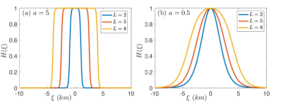
Figure 1: Continuous heterogeneous-in-$\xi$ habitat function $H\big{(}\xi)$ as defined in (2.10) with (a) a steep spatial gradient $a=5\ km^{-1}$ and (b) a gentle spatial gradient $a=0.5\ km^{-1}$. In each panel, the three different colours represent three different lengths $L=2,5$, and $8\ km$.

To motivate our work, we consider two cases for a given $L$. In the case of sufficiently large $a$, there is an abrupt transition between the good and bad habitats, with the length of the good habitat being approximately $L$, and with a relatively short length of the transitional habitat; see Figure 1(a). In this case, the heterogeneous habitat function in (2.10) can be approximated by a piecewise-homogeneous function which greatly simplifies analysis of pulse solutions – we explain this in more detail in Section 3.2. However, in the case of sufficiently small $a$, the transitional habitat extends over relatively wide $\xi$-intervals, and the length of the good habitat is noticeably shorter than $L$; see Figure 1(b). This means that the piecewise-homogeneous approximation is no longer valid, and there is a need for an alternative approach to analyze pulse solutions.

2.2 B-tipping and R-tipping in the habitat model

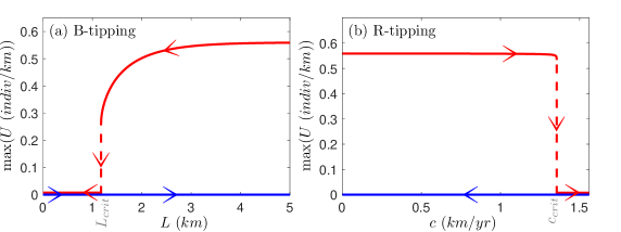
Figure 2: One-parameter attractor diagrams of pulses for the RDE (2.1)–(2.2) with the Allee reaction term (2.9), obtained using the ARDE (2.4)–(2.5) with (2.9). (a) Decreasing (red) and then increasing (blue) the length $L$ of a static habitat ($c=0\ km/yr$) shows B-tipping from a standing pulse to extinction at a critical length $L\approx 1.1748727\ km$. (b) Increasing (red) and then decreasing (blue) the speed $c$ of a moving habitat with a fixed $L_{crit}=5\ km$ shows R-tipping from a travelling pulse to extinction at a critical speed $c_{crit}\approx 1.35536596\ km/yr$. Other parameter values are given in Table 1.

To give a taste of different tipping mechanisms that are present in the habitat model, we perform direct numerical simulations to detect stable pulse solutions in the ARDE (2.4)–(2.5) with the Allee reaction term (2.9) and $U^{\pm}=0$; see Figure 2.

In Figure 2(a), we set $c=0$ and simulate a slowly shrinking habitat. We start with $L=5$, detect a stable standing pulse solution, then decrement $L$, use the previously obtained solution as an initial condition, converge to the new stable solution, and repeat this procedure until we reach $L=0$. The result is a stable branch of standing pulses that terminates at the critical length $L=L_{crit}\approx 1.17537$. For $0<L<L_{crit}$, the system always converges to the extinction solution $U(x)=0$. Subsequently, we increment $L$ using the same procedure, which shows that the branch of extinction solutions is stable, at least up to $L=5$. Thus, the shrinking habitat undergoes B-tipping to extinction upon decreasing $L$, and this transition cannot be reversed by increasing $L$ back to its initial value.

In Figure 2(b), we fix $L=5$ and simulate a geographically shifting habitat at different speeds $c>0$. We start with $c=0$, detect a stable standing pulse solution, then increment $c$, and proceed in the same manner as in Figure 2(a). The result is a stable branch of travelling pulses that terminates at the critical speed $c=c_{crit}\approx 1.35527$. For $c>c_{crit}$, the system always converges to the extinction solution $U(x)=0$. Thus, the moving habitat undergoes R-tipping to extinction above the critical rate $c_{crit}$. Note that, in contrast to the branch of standing pulses near $L_{crit}$ in (a), the branch of travelling pulses in (b) remains nearly constant, showing no indication of the imminent critical speed. In the remainder of the paper, we develop a framework to study pulse solutions in bi-asymptotically homogeneous RDEs and use this framework to uncover and discuss the dynamical mechanisms responsible for both tipping examples in Figure 2.

3 The framework

We here propose a framework that facilitates analysis of travelling pulses and fronts in the heterogeneous and nonautonomous RDE (2.1) or stationary fronts and pulses in the heterogeneous ARDE (2.4). This framework

• is applicable to $C^{1}$-smooth reaction terms that are bi-asymptotically homogeneous in $\xi$, meaning that 

  $$H(\xi)\to h^{\pm}\in\mathbb{R}\;\;\;\mbox{and}\;\;\;f(U,H(\xi))\to f(U,h^{\pm})\;\;\;\mbox{as}\;\;\;\xi\to\pm\infty,$$

  and Dirichlet boundary conditions

  $$\lim_{\xi\to\pm\infty}U(\xi,t)=U^{\pm}\in\mathbb{R};$$

• uses the compactification technique of [66] to transform a pulse or front solution in system (2.1) or (2.4) into a heteroclinic orbit in a suitably compactified system;

• uses Lin’s method [39] implemented in the continuation software package AUTO [14, 30] to compute heteroclinic orbits in the compactified system that correspond to pulse and front solutions in system (2.1) or (2.4).

We introduce this framework in four steps.

3.1 Nondimensionalization

Quantity	Allee rescaling	Allee value	Logistic rescaling	Logistic value
$\mathcal{U}$	$\sqrt{\frac{\gamma}{a^{2}D}}\,U$	$[0,\infty)$	$\frac{\gamma}{a^{2}D}\,U$	$[0,\infty)$
$z$	$a\,\xi$	$(-\infty,\infty)$	$a\,\xi$	$(-\infty,\infty)$
$\tau$	$a^{2}Dt$	$[0,\infty)$	$a^{2}Dt$	$[0,\infty)$
$\tilde{\beta}$	$\sqrt{\frac{\beta}{a^{2}D}}$	varied	$\sqrt{\frac{\beta}{a^{2}D}}$	varied
$\tilde{L}$	$a\,L$	varied	$a\,L$	varied
$\tilde{c}$	$\frac{c}{aD}$	varied	$\frac{c}{aD}$	varied

Table 2: Dimensionless variables and parameters for system (3.1)–(3.2) with $D>0$.

In the first step, summarized in Table 2, we rewrite the BVP (2.6)–(2.7) in terms of a dimensionless moving-frame coordinate $z$ and a dimensionless state variable $\mathcal{U}(z)$ as 

$$\mathcal{U}_{zz}+\tilde{c}\,\mathcal{U}_{z}+\tilde{f}(\mathcal{U},\tilde{H}(z))=0,$$ (3.1)

$$\displaystyle{\lim_{z\to\pm\infty}}\mathcal{U}(z)={\mathcal{U}}^{\pm}\in\mathbb{R}.$$ (3.2)

A particular advantage of this nondimensionalization is that the number of parameters in the system reduces from seven to just three, namely, $\tilde{c}$, $\tilde{\beta}$, and $\tilde{L}$. This advantage becomes clear from the rescaled Allee reaction term (2.9),

$$\tilde{f}_{A}(\mathcal{U},\tilde{H}(z))=\mathcal{U}\left(-\tilde{\beta}^{2}+4\tilde{\beta}\,\tilde{H}(z)\,\mathcal{U}-\mathcal{U}^{2}\right),$$ (3.3)

and the rescaled habitat function (2.10),

$$\tilde{H}(z)=\dfrac{\tanh(z+\tilde{L}/2)-\tanh(z-\tilde{L}/2)}{2\tanh(\tilde{L}/2)}.$$ (3.4)

3.2 Pulses and fronts in the moving-frame ODE

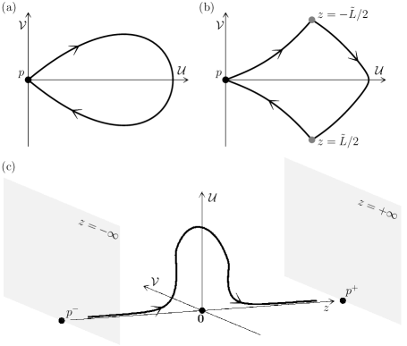
Figure 3: A pulse solution for an RDE can be obtained in the moving-frame ODE by computing (a) a smooth homoclinic orbit to a saddle $p$ when the reaction term is homogeneous ($z$-independent), (b) a piecewise-smooth homoclinic orbit to a saddle $p$ when the reaction term is piecewise-homogeneous (piecewise-constant in $z$), and (c) a trajectory that limits to an equilibrium $p^{\pm}$ as $z$ tends to $\pm\infty$ when the reaction term is bi-asymptotically homogeneous.

In the second step, we rewrite the second-order BVP (3.1)–(3.2) as a first-order BVP at the expense of introducing an additional dependent variable $\mathcal{V}(z)={\mathcal{U}}_{z}(z)$:

$$\mathcal{U}_{z} =\mathcal{V},$$ (3.5)

$$\mathcal{V}_{z} =-\tilde{c}\,\mathcal{V}-\tilde{f}(\mathcal{U},\tilde{H}(z)),$$ (3.6)

$$\displaystyle{\lim_{z\to\pm\infty}}\mathcal{U}(z) ={\mathcal{U}}^{\pm}\in\mathbb{R}.$$ (3.7)

We then view the moving-frame ODEs (3.5) and (3.6) as a dynamical system on $\mathbb{R}^{2}$, where $z$ plays the role of time. The following three paragraphs overview how one can obtain pulse and front solutions to the BVP (3.5)–(3.7) depending on the nature of the reaction term $\tilde{f}$.

In typical problems with a $z$-independent reaction term $\tilde{f}(\mathcal{U},h)$ and a constant $h\in\mathbb{R}$, the ensuing dynamical system is autonomous. Pulse solutions are possible if ${\mathcal{U}}^{\pm}={\mathcal{U}}^{*}$ and there is a saddle equilibrium point $p=({\mathcal{U}}^{*},0)$ in the $(\mathcal{U},\mathcal{V})$ phase plane, in which case such solutions can be computed as homoclinic orbits to $p$; see Figure 3(a). Similarly, front solutions are possible if ${\mathcal{U}}^{-}\neq{\mathcal{U}}^{+}$ and there are two different equilibrium points, $p^{-}=({\mathcal{U}}^{-},0)$ and $p^{+}=({\mathcal{U}}^{+},0)$, in which case such solutions can be computed as heteroclinic orbits from ${p}^{-}$ to ${p}^{+}$. This typical approach has been widely implemented, for example, in [33, Ch.7], [34, Ex.6.3] and [9, 24, 56, 57].

In problems where the reaction term $\tilde{f}(U,\tilde{H}(z))$ can be approximated by a piecewise-homogeneous function, the ensuing dynamical system is piecewise-autonomous. For example, if

$$\tilde{f}(U,\tilde{H}(z))=\begin{cases}\tilde{f}(U,h^{-}),\quad h^{-}\in\mathbb{R},&\text{if}\;\;\;z<-\tilde{L}/2,\\ \tilde{f}(U,h^{0}),\quad\ h^{0}\in\mathbb{R},&\text{if }-\tilde{L}/2\leq z\leq\tilde{L}/2,\\ \tilde{f}(U,h^{+}),\quad h^{+}\in\mathbb{R},&\text{if}\;\;\;z>\tilde{L}/2,\end{cases}$$ (3.8)

the system is given by a set of three (constituent) autonomous dynamical systems that are defined on three adjacent $z$-intervals with shared boundaries at $z=\pm L/2$; see Figure 1(a). Pulse solutions are possible if ${\mathcal{U}}^{\pm}=\mathcal{U}^{*}$ and there is a saddle equilibrium point $p=(\mathcal{U}^{*},0)$ for $z<-\tilde{L}/2$ and $z>\tilde{L}/2$. Then, such solutions can be computed as piecewise-smooth homoclinic orbits to $p$, via a concatenation of three orbit segments of the three constituent autonomous systems that match at ‘times’ $z=\pm\tilde{L}/2$; see Figure 3(b). Similarly, front solutions are possible if ${\mathcal{U}}^{-}\neq{\mathcal{U}}^{+}$ and there are two different equilibrium points, $p^{-}=({\mathcal{U}}^{-},0)$ for $z<-\tilde{L}/2$ and $p^{+}=({\mathcal{U}}^{+},0)$ for $z>\tilde{L}/2$, in which case such solutions can be computed as piecewise-smooth heteroclinic orbits from $p^{-}$ to $p^{+}$. Such a concatenation technique was proposed in [26, 25, 35] and has been implemented in various contexts and applications [6, 28, 46, 62].

By contrast, a general $z$-dependent reaction term $\tilde{f}(\mathcal{U},\tilde{H}(z))$ poses an obstacle to computing pulse and front solutions: it gives rise to a nonautonomous dynamical system (3.5)–(3.6) that has no equilibrium points in the extended $(\mathcal{U},\mathcal{V},z)$ phase space; see Figure 3(c). This obstacle becomes particularly apparent when the BVP (3.5)–(3.7) has multiple ‘nearby’ pulse or front solutions that may be difficult to capture by a shooting method or a collocation method. To overcome this obstacle, we exploit the fact that the reaction term is bi-asymptotically homogeneous in the sense that

$$\tilde{f}(\mathcal{U},\tilde{H}(z))\to\tilde{f}(\mathcal{U},h^{\pm})\quad\mbox{as}\quad z\to\pm\infty.$$

Specifically, we use an equilibrium point

$$p^{-}=(\mathcal{U},\mathcal{V})=({\mathcal{U}}^{-},0),$$

for the autonomous past limit system

$$\begin{split}\mathcal{U}_{z}&=\mathcal{V},\\ \mathcal{V}_{z}&=-\tilde{c}\,\mathcal{V}-\tilde{f}(\mathcal{U},h^{-}),\end{split}$$ (3.9)

and an equilibrium point

$$p^{+}=(\mathcal{U},\mathcal{V})=({\mathcal{U}}^{+},0),$$

for the autonomous future limit system

$$\begin{split}\mathcal{U}_{z}&=\mathcal{V},\\ \mathcal{V}_{z}&=-\tilde{c}\,\mathcal{V}-\tilde{f}(\mathcal{U},h^{+}),\end{split}$$ (3.10)

to construct pulse or front solutions as heteroclinic orbits from $p^{-}$ to $p^{+}$ in a suitably compactified system.

3.3 Compactification

In the third step, we bring in equilibria of the limit systems from infinity by reformulating the nonautonomous system (3.5)–(3.6) on $\mathbb{R}^{2}$ into an autonomous compactified system on $\mathbb{R}^{2}\times[-1,1]$. This requires a suitable coordinate transformation that makes the additional dependent variable bounded and ensures that the compactified system is at least $C^{1}$-smooth on the extended phase space.

Reference [66, Sec. 4] constructs examples of coordinate transformations for different asymptotic decays of the nonautonomous reaction term, ranging from sub-logarithmic to super-exponential decays. Here, we focus on the case where the nonautonomous reaction term decays exponentially with a decay coefficient $\rho>0$ as $z$ tends to $\pm\infty$, in the sense that [65]

$$\lim_{z\to\pm\infty}\frac{\tilde{H}_{z}(z)}{e^{\mp\rho z}}\;\;\mbox{exists for some $\rho>0$}.$$

Thus, we use the parameterized coordinate transformation [66, Eq.(48)], designed for exponentially or faster decaying reaction terms, to augment the nonautonomous system (3.5)–(3.6) with

$$s=g_{\alpha}(z)=\tanh\left(\frac{\alpha}{2}z\right),$$ (3.11)

as a third dependent variable. The compactification parameter $\alpha>0$ quantifies the rate of the exponential decay of both $s(z)$ and $s_{z}(z)$. We note that $s\in(-1,1)$ for $z\in\mathbb{R}$, use the definition of $\tanh^{-1}$ to obtain the inverse transformation

$$z=g_{\alpha}^{-1}(s)=\frac{1}{\alpha}\ln{\frac{1+s}{1-s}},$$ (3.12)

and differentiate $g_{\alpha}(z)$ in (3.11) with respect to $z$ to derive the ODE for $s$:

$$s_{z}=\frac{\alpha}{2}\,(1-s^{2}).$$

Next, we continuously extend the new dependent variable $s$ to include the limits from $z=\pm\infty$, which correspond to $s=\pm 1$. This gives the autonomous compactified system

$$\left\{\begin{array}[]{rrl}\mathcal{U}_{z}&=&\mathcal{V},\\ \mathcal{V}_{z}&=&-\tilde{c}\,\mathcal{V}-\tilde{f}\Big{(}\mathcal{U},\tilde{H}_{\alpha}(s)\Big{)},\\ s_{z}&=&\dfrac{\alpha}{2}(1-s^{2}),\end{array}\right.$$ (3.13)

defined on $\mathbb{R}^{2}\times[-1,1]$, with the continuously-extended habitat function

$$\tilde{H}_{\alpha}(s)=\begin{cases}\tilde{H}(g^{-1}_{\alpha}(s)),&\text{for}\;\;\;s\in(-1,1),\\ h^{-},&\text{for }s=-1,\\ h^{+},&\text{for}\;\;\;s=1.\end{cases}$$ (3.14)

It follows from [66, Cor.4.1] that if $\tilde{H}(z)$ decays exponentially with a decay coefficient $\rho>0$, then the compactified system (3.13) is continuously differentiable on the extended phase space $\mathbb{R}^{2}\times[-1,1]$ for any

$$\alpha\in(0,\rho].$$

In other words, one needs to ensure that the compactification parameter $\alpha$ does not exceed the exponential decay coefficient $\rho$.

A particular advantage of compactification is that the flow-invariant planes of the compactified system (3.13), namely,

$$S^{-}=\mathbb{R}^{2}\times\{-1\}\quad\mbox{and}\quad S^{+}=\mathbb{R}^{2}\times\{1\},$$

contain equilibria $p^{-}$ and $p^{+}$ of the autonomous past (3.9) and future (3.10) limit systems, respectively. When embedded in the extended phase space of the compactified system (3.13), $p^{-}$ becomes

$$\tilde{p}^{-}=(\mathcal{U},\mathcal{V},s)=(\mathcal{U}^{-},0,-1)\in S^{-},$$

and gains one additional eigendirection $v^{-}$ with positive eigenvalue $\alpha>0$, and $p^{+}$ becomes

$$\tilde{p}^{+}=(\mathcal{U},\mathcal{V},s)=(\mathcal{U}^{+},0,1)\in S^{+},$$

and gains one additional eigendirection $v^{+}$ with negative eigenvalue $-\alpha<0$; see [66, Rem. 3.1 and Cor. 4.1]. Thus, a pulse or front solution to the BVP (2.6)–(2.7) can be computed as a heteroclinic connecting orbit from $\tilde{p}^{-}$ to $\tilde{p}^{+}$ in the compactified system (3.13). The computation of such connecting orbits becomes more convenient if

• $v^{-}$ is normal to $S^{-}$ and typical trajectories leave $\tilde{p}^{-}$ along $v^{-}$,

• $v^{+}$ is normal to $S^{+}$ and typical trajectories approach $\tilde{p}^{+}$ along $v^{+}$.

Suppose that ${p}^{-}$ and ${p}^{+}$ are hyperbolic and note from the discussion of additional eigenvalues due to compactification that $\tilde{p}^{-}$ and $\tilde{p}^{+}$ must be hyperbolic too. If the unstable (stable) invariant manifold of $\tilde{p}^{-}$ ($\tilde{p}^{+}$) is of dimension one, conditions (i) and (ii) are satisfied for any $\alpha\in(0,\rho)$; see [66, Rem. 3.1 and Cor. 4.1] and [65, Prop.6.3]. In contrast, if the unstable invariant manifold of $\tilde{p}^{-}$ is of dimension greater than one, condition (i) is satisfied for any $\alpha\in\left(0,\min\{\rho,l^{-}\}\right)$, where $l^{-}$ is the smallest-magnitude eigenvalue within the unstable eigenspace of $p^{-}$ in the autonomous past limit system (3.9); see [65, Prop.6.3]. Similarly, if the stable invariant manifold of $\tilde{p}^{+}$ is of dimension greater than one, condition (ii) is satisfied for any $\alpha\in\left(0,\min\{\rho,|l^{+}|\}\right)$, where $l^{+}$ is the smallest-magnitude eigenvalue within the stable eigenspace of $p^{+}$ in the autonomous future limit system (3.10).

3.4 Numerical implementation

In the fourth step, we outline a numerical setup for computing pulse and front solutions in a reaction-diffusion system (2.1) or (2.4) as heteroclinic orbits from $\tilde{p}^{-}\in S^{-}$ to $\tilde{p}^{+}\in S^{+}$ in the autonomous compactified system (3.13). For convenience, we use the continuation software package AUTO [14], which allows numerical continuation of solutions to autonomous ODEs subject to boundary conditions.

We start with the notation and write

$$\Gamma(z)=\left(\mathcal{U}(z),\mathcal{V}(z),s(z)\right)\in\mathbb{R}^{2}\times[-1,1],$$

to denote a solution to the compactified system (3.13) at ‘time’ $z$. Furthermore, we write $E^{u}(\tilde{p}^{-})$ to denote the unstable eigenspace of $\tilde{p}^{-}$, $W^{u}(\tilde{p}^{-})$ to denote a (numerical approximation of a local) unstable manifold of $\tilde{p}^{-}$, $E^{s}(\tilde{p}^{+})$ to denote the stable eigenspace of $\tilde{p}^{+}$, and $W^{s}(\tilde{p}^{+})$ to denote a (numerical approximation of a local) stable manifold of $\tilde{p}^{+}$ in (3.13).

A heteroclinic orbit from $\tilde{p}^{-}$ to $\tilde{p}^{+}$ in (3.13) is a special orbit that connects $\tilde{p}^{-}$ to $\tilde{p}^{+}$ along an intersection of $W^{u}(\tilde{p}^{-})$ and $W^{s}(\tilde{p}^{+})$. Such a connection can be approximated by a finite-time orbit segment that starts from $E^{u}(\tilde{p}^{-})$ sufficiently close to $\tilde{p}^{-}$ at time $z=0$, and crosses $E^{s}(\tilde{p}^{+})$ sufficiently close to $\tilde{p}^{+}$ at some later time $z=Z>0$. Specifically, for fixed $\varepsilon^{-},\varepsilon^{+}>0$, we consider a finite-time orbit segment

$$\Gamma:=\left\{\Gamma(z)~{}:~{}z\in[0,Z]\right\}\subset\mathbb{R}^{2}\times[-1,1],$$ (3.15)

where

$$\left\{\begin{array}[]{ll}\Gamma(0)&\in E^{u}(\tilde{p}^{-})\quad\mbox{and}\quad\left\|\Gamma(0)-\tilde{p}^{-}\right\|=\varepsilon^{-},\\ \Gamma(Z)&\in E^{s}(\tilde{p}^{+})\quad\mbox{and}\quad\left\|\Gamma(Z)-\tilde{p}^{+}\right\|=\varepsilon^{+}.\end{array}\right.$$ (3.16)

In other words, $\Gamma(0)$ lies on a half $(n-1)$-sphere of radius $\varepsilon^{-}$ about $\tilde{p}^{-}$ within an $n$-dimensional $E^{u}(\tilde{p}^{-})$, and $\Gamma(Z)$ lies on a half $(m-1)$-sphere of radius $\varepsilon^{+}$ about $\tilde{p}^{+}$ within an $m$-dimensional $E^{u}(\tilde{p}^{-})$. Moreover, $\varepsilon^{-}$ and $\varepsilon^{+}$ are chosen small enough so that $E^{u}(\tilde{p}^{-})$ is a good approximation of $W^{u}(\tilde{p}^{-})$ on the half $(n-1)$-sphere about $\tilde{p}^{-}$, and $E^{s}(\tilde{p}^{+})$ is a good approximation of $W^{s}(\tilde{p}^{+})$ on the half $(m-1)$-sphere of about $\tilde{p}^{+}$.

To obtain such finite-time orbit segments, we implement Lin’s method [39] in AUTO [14]; see also [1, 17, 30, 44, 45, 49, 70]. First, we need to identify a two-dimensional cross section $\Sigma$ that is transversal to the flow along the heteroclinic orbit and, for practical purposes, is sufficiently far from both $\tilde{p}^{-}$ and $\tilde{p}^{+}$. We note that $s_{z}=\alpha/2>0$ at $s=0$ and choose

$$\Sigma:=\{(\mathcal{U},\mathcal{V},s)~{}:~{}s=0\}=\mathbb{R}^{2}\times\{0\},$$ (3.17)

which satisfies the transversality requirement.

Second, we compute two orbit segments, denoted $\Gamma^{-}$ and $\Gamma^{+}$. We define $\Gamma^{-}$ as an orbit segment that starts at time $z=0$ from an $(n-1)$-sphere about $\tilde{p}^{-}$ within $E^{u}(\tilde{p}^{-})$ and meets $\Sigma$ at time $z=Z^{-}>0$:

$$\Gamma^{-}:=\left\{\Gamma^{-}(z)~{}:~{}z\in[0,Z^{-}]\right\}\subset\mathbb{R}^{2}\times[-1,0],$$

where

$$\left\{\begin{array}[]{lll}\Gamma^{-}(0)&\in&E^{u}(\tilde{p}^{-})\quad\mbox{and}\quad\left\|\Gamma^{-}(0)-\tilde{p}^{-}\right\|=\varepsilon^{-},\\ \Gamma^{-}(Z^{-})&\in&\Sigma.\end{array}\right.$$ (3.20)

Going backward in $z$, we define $\Gamma^{+}$ as an orbit segment that starts at ‘time’ $z=0$ from an $(m-1)$-sphere about $\tilde{p}^{+}$ within $E^{s}(\tilde{p}^{+})$ and meets $\Sigma$ at ‘time’ $z=Z^{+}<0$:

$$\Gamma^{+}:=\left\{\Gamma^{+}(z)~{}:~{}z\in[Z^{+},0]\right\}\subset\mathbb{R}^{2}\times[0,1],$$

where

$$\left\{\begin{array}[]{lll}\Gamma^{+}(0)&\in&E^{s}(\tilde{p}^{+})\quad\mbox{and}\quad\left\|\Gamma^{+}(0)-\tilde{p}^{+}\right\|=\varepsilon^{+},\\ \Gamma^{+}(Z^{+})&\in&\Sigma.\end{array}\right.$$ (3.21)

The computation of these two orbit segments can be performed by the shooting method, that is, by reducing the BVP to an IVP and solving the IVP using direct $z$-integration. Here, we use AUTO instead, which solves the BVP directly by combining an adaptive collocation method [55] and pseudoarclength continuation [13]. One advantage of our approach is to equidistribute the local discretization error along the computed orbit segment. Another advantage is that once an orbit segment satisfying (3.20) or (3.21) is computed in AUTO, it can be readily numerically continued in AUTO by varying a system parameter or a parameterized boundary condition. To be more precise, in the case where the eigenspace $E^{u}(\tilde{p}^{-})$ is one-dimensional, the boundary condition $\Gamma^{-}(0)$ is fixed at a half zero-sphere (a single point) within $E^{u}(\tilde{p}^{-})$, a distance $\varepsilon^{-}$ from $\tilde{p}^{-}$. Similarly, if $E^{s}(\tilde{p}^{+})$ is one-dimensional, the boundary condition $\Gamma^{+}(0)$ is fixed at a single point within $E^{s}(\tilde{p}^{+})$, a distance $\varepsilon^{+}$ from $\tilde{p}^{+}$. However, in the case where the eigenspace $E^{u}(\tilde{p}^{-})$ is two-dimensional, the boundary condition $\Gamma^{-}(0)$ is contained in a half one-sphere (a half circle) of radius $\varepsilon^{-}$ about $\tilde{p}^{-}$ within $E^{u}(\tilde{p}^{-})$. Similarly, if $E^{s}(\tilde{p}^{+})$ is two-dimensional, the boundary condition $\Gamma^{+}(0)$ is contained in a half circle of radius $\varepsilon^{+}$ about $\tilde{p}^{+}$ within $E^{s}(\tilde{p}^{+})$. Thus, when $E^{u}(\tilde{p}^{-})$ or $E^{s}(\tilde{p}^{+})$ is two-dimensional, we parameterise the boundary condition $\Gamma^{-}(0)$ on the respective half circle by an angle parameter $\theta^{-}\in(0,\pi)$, and $\Gamma^{+}(0)$ on the respective half circle by an angle parameter $\theta^{+}\in(0,\pi)$.

Third, we proceed to close the so-called Lin’s gap, which is defined as the Euclidean distance between the end points $\Gamma^{-}(Z^{-})$ and $\Gamma^{+}(Z^{+})$ in $\Sigma$:

$$\eta=\left\|\Gamma^{-}(Z^{-})-\Gamma^{+}(Z^{+})\right\|.$$

We are interested in structurally-stable (observable) pulse and front solutions, which typically correspond to codimension-zero heteroclinic orbits from $\tilde{p}^{-}$ to $\tilde{p}^{+}$, meaning that such connections persist on an open set of system parameters. Hence, we close the Lin’s gap by varying parameterized boundary conditions rather than system parameters. For example, when $W^{u}(\tilde{p}^{-})$ and $W^{s}(\tilde{p}^{+})$ are both two dimensional, their transverse intersections are codimension-zero heteroclinic orbits, and we close the Lin’s gap by varying $\theta^{-}$ and $\theta^{+}$. The strategy is to fix $\varepsilon^{-}$ and $\varepsilon^{+}$, solve the BVP (3.13) and (3.20) with a suitable choice of $\theta^{-}$, solve the BVP (3.13) and (3.21) with a suitable choice of $\theta^{+}$, and then vary $\theta^{-}$ and $\theta^{+}$ simultaneously and monitor the Lin’s gap $\eta$. Once the Lin’s gap is closed, meaning that $\eta=0$ and $\Gamma^{-}(Z^{-})=~{}\Gamma^{+}(Z^{+})$, we concatenate $\Gamma^{-}$ and $\Gamma^{+}$ to obtain a single orbit segment $\Gamma$ that satisfies the desired BVP (3.13) and (3.16) and has a finite integration time of $Z=Z^{-}-Z^{+}$. In this way, we can approximate a single heteroclinic orbit from $\tilde{p}^{-}$ to $\tilde{p}^{+}$ in (3.13), which corresponds to a pulse or front solution in (2.1) or (2.4).

In the case where both eigenspaces $E^{u}(\tilde{p}^{-})$ and $E^{s}(\tilde{p}^{+})$ are of dimension two, there can be multiple coexisting heteroclinic orbits from $\tilde{p}^{-}$ to $\tilde{p}^{+}$. To capture multiple coexisting heteroclinic orbits, we proceed as follows. We write $\Gamma^{-}_{\theta^{-}}$ and $\Gamma^{+}_{\theta^{+}}$ to indicate the dependence of the orbit segments $\Gamma^{-}$ and $\Gamma^{+}$ on the angle parameters $\theta^{-}$ and $\theta^{+}$. Numerical continuation in $\theta^{-}$ of an orbit segment $\Gamma^{-}_{\theta^{-}}$ satisfying (3.20) gives a parameterized family of orbit segments

$$W^{u}(\tilde{p}^{-}):=\{\Gamma^{-}_{\theta^{-}}~{}:~{}\theta^{-}\in(0,\pi)\},$$

which approximates the two-dimensional local unstable manifold of $\tilde{p}^{-}$. Similarly, numerical continuation in $\theta^{+}$ of an orbit segment $\Gamma^{+}_{\theta^{+}}$ satisfying (3.21) gives a parameterized family of orbit segments

$$W^{s}(\tilde{p}^{+}):=\{\Gamma^{+}_{\theta^{+}}~{}:~{}\theta^{+}\in(0,\pi)\},$$

which approximates the two-dimensional local stable manifold of $\tilde{p}^{+}$. $W^{u}(\tilde{p}^{-})$ and $W^{s}(\tilde{p}^{+})$ each intersects the cross section $\Sigma$ along a different curve. Typically, these two curves intersect each other at isolated points in $\Sigma$. Each such isolated point in $\Sigma$ approximates an intersection of $\Sigma$ with a different heteroclinic orbit from $\tilde{p}^{-}$ to $\tilde{p}^{+}$. For each such isolated point in $\Sigma$, a finite-time approximation $\Gamma$ to the corresponding heteroclinic orbit is obtained by a concatenation of the two orbit segments, $\Gamma^{-}$ and $\Gamma^{+}$, that meet at this point.

Furthermore, in the case of multiple coexisting heteroclinic orbits from $\tilde{p}^{-}$ to $\tilde{p}^{+}$, there is a possibility that some connections become degenerate, for example, along a (codimension-one) tangency of $W^{u}(\tilde{p}^{-})$ and $W^{s}(\tilde{p}^{+})$, as the system parameters are varied. Such degeneracies of heteroclinic orbits in the compactified system (3.13) correspond to bifurcations of pulse and front solutions in a reaction-diffusion system (2.1) or (2.4). Bifurcations of travelling waves is an area of great interest; see, for example, [20, 56, 57]. A particular advantage of our framework is that these bifurcations can be detected by numerical continuation of the orbit segment $\Gamma$ in one of the system parameters in AUTO. Once detected, these bifurcations can be then continued in two system parameters to produce two-parameter bifurcation diagrams of pulse and front solutions.

4 Pulse solutions and their bifurcations in the habitat model

In this section, we study the existence and bifurcations of pulse solutions in the geographically shifting habitat model (2.1)–(2.2), or equivalently (2.4)–(2.5), with

$$u^{\pm}=U^{\pm}=0,$$ (4.1)

the Allee reaction term (2.9), and the habitat function (2.10). Specifically, we use the framework outlined in section 3 to obtain pulse solutions for the habitat model by computing heteroclinic orbits in the nondimensionalized compactified system

$$\left\{\begin{array}[]{rrl}\mathcal{U}_{z}&=&\mathcal{V},\\ \mathcal{V}_{z}&=&-\tilde{c}\,\mathcal{V}-\tilde{f}_{A}\Big{(}\mathcal{U},\tilde{H}_{\alpha}(s)\Big{)},\\ s_{z}&=&\dfrac{\alpha}{2}(1-s^{2}).\end{array}\right.$$ (4.2)

Here, the dimensionless Allee reaction term (3.3) is given in terms of $s$ instead of $z$,

$$\tilde{f}_{A}\Big{(}\mathcal{U},\tilde{H}_{\alpha}(s)\Big{)}=-\tilde{\beta}^{2}\mathcal{U}+4\tilde{\beta}\,\tilde{H}_{\alpha}(s)\,\mathcal{U}^{2}-\mathcal{U}^{3},$$ (4.3)

using the rescaled and extended habitat function $\tilde{H}_{\alpha}(s)$ from (3.14) with $h^{\pm}=0$ and

$$\tilde{H}(g^{-1}_{\alpha}(s))=\frac{e^{\tilde{L}}-e^{-\tilde{L}}}{\tanh\left(\frac{\tilde{L}}{2}\right)\left(e^{\tilde{L}}\ +e^{-\tilde{L}}+\left(\frac{1+s}{1-s}\right)^{\frac{2}{\alpha}}+\left(\frac{1-s}{1+s}\right)^{\frac{2}{\alpha}}\right)},$$ (4.4)

which is derived by employing the inverse coordinate transformation (3.12) to express $z$ in terms of $s$ in the rescaled habitat function (3.4). The compactified logistic model is given in section A.1.

4.1 Equilibria and their stability in the compactified habitat model

We consider the two extinction equilibria for the compactified system (4.2), namely,

$$\tilde{p}^{-}=(\mathcal{U},\mathcal{V},s)=(0,0,-1)\in S^{-},$$

and

$$\tilde{p}^{+}=(\mathcal{U},\mathcal{V},s)=(0,0,1)\in S^{+},$$

which correspond to $u^{\pm}=0$ in (2.2), or equivalently to $U^{\pm}=0$ in (2.5). Next, we note that the rescaled habitat function $\tilde{H}(z)$ in (3.4) decays exponentially to zero with a decay coefficient $\rho=2$ as $z\to\pm\infty$. Hence, we need to choose the compactification parameter

$$\alpha\in(0,2],$$

to ensure that the compactified system (4.2) is C¹-smooth (continuously differentiable) at the added invariant planes $S^{-}$ containing $\tilde{p}^{-}$ and $S^{+}$ containing $\tilde{p}^{+}$; see section 3.3 and the references therein. Linear stability analysis shows that $\tilde{p}^{-}$ is a saddle with eigenvalues

$$l^{-}_{1}=\frac{-\tilde{c}-\sqrt{\tilde{c}^{2}+4\tilde{\beta}^{2}}}{2}<0,\quad l^{-}_{2}=\frac{-\tilde{c}+\sqrt{\tilde{c}^{2}+4\tilde{\beta}^{2}}}{2}>0,\quad\mbox{and}\quad l^{-}_{3}=\alpha>0,$$

meaning that it has a two-dimensional local unstable invariant manifold $W^{u}(\tilde{p}^{-})$. Similarly, $\tilde{p}^{+}$ is a saddle with eigenvalues

$$l^{+}_{1}=l^{-}_{1}<0,\quad l^{+}_{2}=l^{-}_{2}>0,\quad\mbox{and}\quad l^{+}_{3}=-l^{-}_{3}=-\alpha<0,$$

meaning that it has a two-dimensional local stable invariant manifold $W^{s}(\tilde{p}^{+})$. Next, we note that $l_{2}^{-}\leq|l_{1}^{+}|$ and, for practical convenience, we limit the choices for the compactification parameter to

$$\alpha\in\left(0,\min\{2,l^{-}_{2},|l_{1}^{+}|\}\right),\quad\text{or equivalently}\quad\alpha\in\left(0,\min\{2,l^{-}_{2}\}\right),$$

to ensure that the additional eigenvector $v^{-}_{3}$ (corresponding to $l^{-}_{3}$) is normal to $S^{-}$, the additional eigenvector $v^{+}_{3}$ (corresponding to $l^{+}_{3}$) is normal to $S^{+}$, and typical trajectories leave $\tilde{p}^{-}$ along $v^{-}_{3}$ and approach $\tilde{p}^{+}$ along $v^{+}_{3}$; see section 3.3 and the references therein. We then note that, for $\tilde{c}\geq 0$ and $\tilde{\beta}<2$, $l_{2}^{-}\in(0,\tilde{\beta}]$ if and only if $D>4.5\times 10^{-3}$. Hence we choose

$$\alpha=\begin{cases}l_{2}^{-}/2,&\text{if}\;\;\;D>4.5\times 10^{-3},\\ 1,&\text{if}\;\;\;0<D<4.5\times 10^{-3}.\end{cases}$$ (4.5)

We fix all the model parameters in Table 1, except for $L$, $c$, and $D$, which could be varied. Although we work with the nondimensionalized compactified system (4.2), we specify the original parameters as input parameters in all figures.

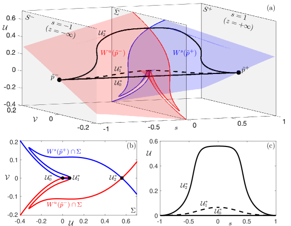
Figure 4: Standing-pulse solutions for the RDE (2.1)–(2.2) with the Allee reaction term (2.9) obtained by computing intersections of two-dimensional invariant manifolds $W^{u}(\tilde{p}^{-})$ and $W^{s}(\tilde{p}^{+})$ in the compactified moving-frame ODE (4.2) with the $s$-dependent Allee reaction term (4.3). (a) The unstable invariant manifold $W^{u}(\tilde{p}^{-})$ of saddle $\tilde{p}^{-}$ (red surface), the stable invariant manifold $W^{s}(\tilde{p}^{+})$ of saddle $\tilde{p}^{+}$ (blue surface), intersections of $W^{u}(\tilde{p}^{-})$ and $W^{s}(\tilde{p}^{+})$ with the cross section $\Sigma$ (3.17) (red and blue curves, respectively), and transverse heteroclinic intersections of $W^{u}(\tilde{p}^{-})$ with $W^{s}(\tilde{p}^{+})$ (black curves $\mathcal{U}_{0}^{*}$, $\mathcal{U}_{1}^{*}$, and $\mathcal{U}_{2}^{*}$). (b) The cross section $\Sigma$ from (a). (c) The stable extinction state $\mathcal{U}_{0}^{*}$, the unstable standing pulse $\mathcal{U}_{1}^{*}$, and the stable standing pulse $\mathcal{U}_{2}^{*}$, shown over the compactified dimensionless space coordinate $s$. We used $c=0\ km/yr$, $D=~{}0.8\ km^{2}/yr$, and $L=5\ km$; other parameter values are given in table 1.

4.2 Pulse solutions as heteroclinic orbits in the compactified system

Codimension-zero heteroclinic orbits from $\tilde{p}^{-}$ to $\tilde{p}^{+}$ along transverse intersections of $W^{u}(\tilde{p}^{-})$ and $W^{s}(\tilde{p}^{+})$ in the extended phase space $\mathbb{R}\times[-1,1]$ of compactified system (4.2) correspond to structurally-stable pulse solutions in the habitat model, whereas codimension-one heteroclinic orbits along tangent intersections of $W^{u}(\tilde{p}^{-})$ and $W^{s}(\tilde{p}^{+})$ correspond to bifurcations of pulse solutions; see section 3.4 for more details. Numerically, we approximate both types of heteroclinic orbits using a finite-time orbit segment (3.15) with boundary conditions (3.16) parameterized by the angles $\theta^{-}$ and $\theta^{+}$ as follows:

$$\left\{\begin{array}[]{lcr}\Gamma(0)&=&\tilde{p}^{-}+\varepsilon^{-}(v^{-}_{2}\cos\theta^{-}+v^{-}_{3}\sin\theta^{-}),\\ \Gamma(Z)&=&\tilde{p}^{+}+\varepsilon^{+}(v^{+}_{1}\cos\theta^{+}+v^{+}_{3}\sin\theta^{+}).\end{array}\right.$$ (4.6)

Here, the unit eigenvectors $v^{-}_{2}$ and $v^{-}_{3}$ correspond to the eigenvalues $l^{-}_{2}$ and $l^{-}_{3}$ and span the unstable eigenspace $E^{u}(\tilde{p}^{-})$. The unit eigenvectors $v^{+}_{1}$ and $v^{+}_{3}$ correspond to the eigenvalues $l^{+}_{1}$ and $l^{+}_{3}$ and span the stable eigenspace $E^{s}(\tilde{p}^{+})$. To ensure that $s\in(-1,1)$ for $\Gamma(0)$ and $\Gamma(Z)$, we use $\theta^{\pm}\in(0,\pi)$; see section 3.4.

To compute multiple coexisting heteroclinic orbits from $\tilde{p}^{-}$ to $\tilde{p}^{+}$, we use the numerical setup described in the last two paragraphs of section 3.4. The results shown in Figure 4 include (a)-(b) intersecting two-dimensional invariant manifolds $W^{u}(\tilde{p}^{-})$ and $W^{s}(\tilde{p}^{+})$, together with (c) the corresponding dimensionless pulse solutions $\mathcal{U}^{*}(s)$. In panel (a), we plot the (light red) unstable manifold $W^{u}(\tilde{p}^{-})$ of $\tilde{p}^{-}\in S^{-}$ and the (light blue) stable manifold $W^{s}(\tilde{p}^{+})$ of $\tilde{p}^{+}\in S^{+}$, each computed up to the (grey) two-dimensional cross section $\Sigma$ defined in (3.17). The invariant manifolds $W^{u}(\tilde{p}^{-})$ and $W^{s}(\tilde{p}^{+})$ each intersect $\Sigma$ along a different curve. The (dark red) intersection curve $W^{u}(\tilde{p}^{-})\cap\Sigma$ and the (dark blue) intersection curve $W^{s}(\tilde{p}^{+})\cap\Sigma$ are shown in more detail in Figure 4(b). These two curves intersect each other in three isolated (black) points in $\Sigma$, labelled $\mathcal{U}_{0}^{*}$, $\mathcal{U}_{1}^{*}$, and $\mathcal{U}_{2}^{*}$. Each of these points corresponds to an intersection of a different heteroclinic orbit from $\tilde{p}^{-}$ to $\tilde{p}^{+}$ with $\Sigma$. The three heteroclinic orbits are shown (in black) in the projection onto ($s,\mathcal{U}$)-plane in panel (c).

In the habitat model (2.1)–(2.2), the trivial heteroclinic orbit $\mathcal{U}^{*}_{0}=0$ corresponds to the extinction state, which is stable. The nontrivial heteroclinic orbits $\mathcal{U}^{*}_{1}$ and $\mathcal{U}^{*}_{2}$ correspond to pulses that are standing when $c=0$, or travelling when $c>0$; see Figure 4(c). Pulse $\mathcal{U}^{*}_{2}$ represents the carrying capacity of the habitat and is stable. Pulse $\mathcal{U}^{*}_{1}$ is unstable and is contained in the (infinite-dimensional) Allee threshold, which separates initial states that converge to extinction $\mathcal{U}^{*}_{0}$ from those that converge to the carrying capacity $\mathcal{U}^{*}_{2}$.

4.3 B-tipping in a shrinking habitat: Critical length

Here, we consider a static habitat with $c=0$, meaning the the original space coordinate and the moving-frame coordinate are identical, that is, $x=\xi$. Thus, the new variable $s$ in (3.11) can be interpreted as a compactified and rescaled original coordinate $x$:

$$s=\tanh\left(\frac{1}{4}\sqrt{\frac{\beta}{D}}\,x\right).$$

Our aim is to describe standing-pulse solutions in the habitat model (2.1)–(2.2) and how they depend on $L$. To start with, we compute branches of standing pulses in (2.1)–(2.2) by performing numerical continuation of nontrivial heteroclinic orbits in parameter $L$ in the compactified system (4.2). The ensuing one-parameter bifurcation diagram for the Allee reaction term (4.3) is shown in Figure 5(a). The stable extinction state $\mathcal{U}^{*}_{0}$ exists for all $L>0$ and is the only stationary solution for $L$ sufficiently small. As $L$ is increased, there is a saddle-node (SN) bifurcation of standing pulses at some critical length $L=L_{crit}$. This bifurcation gives rise to two standing pulses that exist for $L>L_{crit}$, namely, the unstable pulse $\mathcal{U}^{*}_{1}$ and the stable carrying-capacity pulse $\mathcal{U}^{*}_{2}$, and explains the the attractor diagram in Figure 2(a).

Now consider a shrinking-habitat scenario during which $L(t)$ slowly decreases over time, for example, due to deforestation and changes in land use by the growing human population. We expect that the ecosystem, represented by the red trajectory in Figure 5(a), tracks the stable branch of changing carrying-capacity base states $\mathcal{U}^{*}_{2}$ until $L(t)$ reaches its critical value $L_{crit}$. At this bifurcation point the carrying-capacity base state $\mathcal{U}^{*}_{2}$ disappears. The ensuing discontinuity in the stable branch of base states gives rise to a sudden transition to the alternative stable state, namely, the extinction state $\mathcal{U}^{*}_{0}$. This transition is an example of B-tipping because it is caused solely by a dangerous bifurcation of standing pulses and occurs no matter how slowly $L$ decreases. Ecologically speaking, a habitat with $L<L_{crit}$ becomes too small to support population growth: dispersion brings the habitat population below the Allee threshold, leading to extinction.

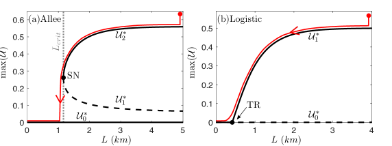
Figure 5: One-parameter bifurcation diagrams of standing pulses for the RDE (2.1)–(2.2) obtained by numerical continuation of heteroclinic orbits in the compactified moving-frame ODE. (a) In the Allee model (4.2)–(4.3) with $c=0\ km/yr$ and $D=0.8\ km^{2}/yr$, the branches of stable pulses $\mathcal{U}^{*}_{2}$ (solid black curve) and unstable pulses $\mathcal{U}^{*}_{1}$ (dashed black curve) meet and terminate in a saddle-node (SN) bifurcation (black dot), while the extinction solution $\mathcal{U}^{*}_{0}=0$ (solid black line) is stable for all values of $L$; compare with fig. 2(a). (b) In the logistic model (A.1)–(A.2) with $c=0\ km/yr$ and $D=0.4\ km^{2}/yr$, the branch of stable pulses $\mathcal{U}^{*}_{1}$ (solid black curve) meets the extinction solution $\mathcal{U}^{*}_{0}=0$ and terminates in a transcritical (TR) bifurcation (black dot), where $\mathcal{U}^{*}_{0}$ changes stability. Red trajectories are the expected solutions of the system when $L$ is decreased slowly. Other parameter values are given in table 1.

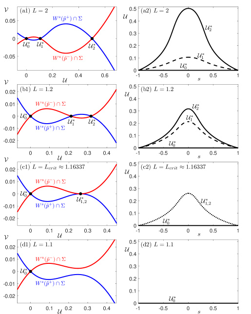
Figure 6: B-tipping in a shrinking habitat RDE (2.1)–(2.2) with the Allee reaction term (2.9) shown as (left column) changing intersections of the (blue) stable and (red) unstable invariant manifolds on the cross section $\Sigma$ (3.17) in the compactified moving-frame ODE (4.2)–(4.3) with $c=0\ km/yr$ and $D=0.8\ km^{2}/yr$ and (right column) colliding (solid curves) stable and (dashed curves) unstable standing pulses, (a)–(b) before, (c) at, and (d) after a SN bifurcation of standing pulses $\mathcal{U}^{*}_{1}$ and $\mathcal{U}^{*}_{2}$. Other parameter values are given in table 1.

The critical length $L_{crit}$ can be detected by finding $L$ that gives a codimension-one heteroclinic orbit along a tangent intersection of $W^{u}(\tilde{p}^{-})$ and $W^{s}(\tilde{p}^{+})$ in the compactified system (4.2). This is shown in more detail in Figure 6. The left column of Figure 6 shows the interplay between the unstable invariant manifold $W^{u}(\tilde{p}^{-})$ and the stable invariant manifold $W^{s}(\tilde{p}^{+})$ on the two-dimensional cross section $\Sigma$ in the compactified system (4.2). The right column of Figure 6 shows the rescaled stationary solutions $\mathcal{U}^{*}(s)$ of the habitat model (2.1)–(2.2) that correspond to the intersections of $W^{u}(\tilde{p}^{-})$ and $W^{s}(\tilde{p}^{+})$. For $L>L_{crit}$, the stable and unstable invariant manifolds intersect transversally in the three points marked with black dots; see Figure 6(a1) and (b1). These intersections give rise to three codimension-zero heteroclinic orbits. These orbits correspond to one trivial solution $\mathcal{U}^{*}_{0}(s)$ that exists for $L>0$, and two standing pulses $\mathcal{U}^{*}_{1}(s)$ and $\mathcal{U}^{*}_{2}(s)$; see Figure 6(a2) and (b2). The situation is different when $L$ reaches a critical level $L=L_{crit}\approx 1.16337$. In addition to the transverse intersection of the manifolds at the origin, there is a tangent intersection away from the origin. This tangent intersection gives rise to a codimension-one heteroclinic orbit, which corresponds to a saddle-node (SN) bifurcation of standing pulses, where $\mathcal{U}^{*}_{1}(s)$ and $\mathcal{U}^{*}_{2}(s)$ coalesce into $\mathcal{U}^{*}_{1,2}(s)$; see Figure 6(c1) and (c2). For $L<L_{crit}$, there is only one transverse intersection of the manifolds at the origin, meaning that $\mathcal{U}^{*}_{0}(s)$ is the only stationary solution for the habitat model; see Figure 6(d1) and (d2).

For comparison, we show the one-parameter bifurcation diagram for the logistic growth model (A.1)–(A.2) in Figure 5(b). As $L$ is increased, there is a transcritical (TR) bifurcation of standing pulses, in which a branch of stable carrying-capacity pulses $\mathcal{U}^{*}_{1}$ bifurcates from the branch of stable extinction states $\mathcal{U}^{*}_{0}$, while $\mathcal{U}^{*}_{0}$ turns unstable. The main difference from the Allee reaction term is that TR is a safe bifurcation, meaning that there is no discontinuity in the branch of stable solutions at TR. There is no critical level $L=L_{crit}$ or bistability either. Thus, when $L(t)$ slowly decreases over time, the (red trajectory) ecosystem tracks the branch of changing carrying-capacity base states $\mathcal{U}^{*}_{1}$ and declines toward the alternative extinction state $\mathcal{U}^{*}_{0}$ gradually, that is, without any sudden transitions. In other words, there is no tipping point for the logistic reaction term.

4.4 R-tipping in a moving habitat: Critical speed

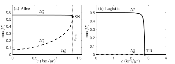
Figure 7: One-parameter bifurcation diagrams of travelling pulses for the RDE (2.1)–(2.2) obtained by numerical continuation of heteroclinic orbits in the compactified moving-frame ODE; refer to fig. 5 for more details. (a) The Allee model (4.2)–(4.3) with $L=5\ km$ and $D=0.8\ km^{2}/yr$; compare with fig. 2(b). (b) The logistic model (A.1)–(A.2) with $L=5\ km$ and $D=0.4\ km^{2}/yr$. Other parameter values are given in table 1.

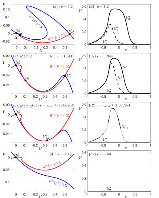
Figure 8: R-tipping in a shifting habitat RDE (2.1)–(2.2) with the Allee reaction term (2.9) shown as (left column) changing intersections of the (blue) stable and (red) unstable invariant manifolds on the cross section $\Sigma$ (3.17) in the compactified moving-frame ODE (4.2)–(4.3) with $D=0.8\ km^{2}/yr$ and $L=5\ km$ and (right column) colliding (solid curves) stable and (dashed curves) unstable travelling pulses, (a)–(b) before, (c) at, and (d) after a SN bifurcation of travelling pulses. Other parameter values are given in table 1.

Here, we fix $L=5>L_{crit}$ and consider a habitat that is moving at a constant speed $c>0$, for example, due to changing weather patterns and ensuing geographical shifts in vegetation communities. Thus, the new variable $s$ in (3.11) can be interpreted as a compactified and rescaled moving-frame coordinate $\xi=x-ct$:

$$s=\tanh\left(\frac{-c+\sqrt{c^{2}+4\beta D}}{8D}\,(x-ct)\right).$$

Our aim is to describe travelling-pulse solutions in the habitat model (2.1)–(2.2) and how they depend on $c$. To start with, we compute branches of travelling pulses in (2.1)–(2.2) by performing numerical continuation of nontrivial heteroclinic orbits in parameter $c$ in the compactified system. The ensuing one-parameter bifurcation diagram for the Allee model (4.2)–(4.3) is shown in Figure 7(a). The stable extinction state $\mathcal{U}^{*}_{0}$ exists for all $c\geq 0$. For $c>0$ sufficiently small, there are two travelling pulses in addition to $\mathcal{U}^{*}_{0}$, namely, an unstable pulse $\mathcal{U}^{*}_{1}$ and a stable carrying-capacity pulse $\mathcal{U}^{*}_{2}$ that represents the ability of an ecosystem to track the moving habitat. Interestingly, as $c$ is increased, the amplitude of the stable carrying-capacity pulse $\mathcal{U}^{*}_{2}$ remains nearly unchanged, while the amplitude of the unstable pulse $\mathcal{U}^{*}_{1}$ increases. Then, at some critical speed $c=c_{crit}$, there is an SN bifurcation of travelling pulses, at which $\mathcal{U}^{*}_{2}$ and $\mathcal{U}^{*}_{1}$ meet and disappear. For $c>c_{crit}$, the ecosystem always goes extinct since $\mathcal{U}^{*}_{0}$ is the only stable state, which explains the attractor diagram in Figure 2(b). This is an example of R-tipping because extinction is caused entirely by the rate of change in the position of the otherwise stable ecosystem. In other words, the spatial position of a static habitat patch in the infinite domain has no effect on the stability of the carrying-capacity base state $\mathcal{U}^{*}_{2}$. Rather, it is the rate of change in the spatial position of the habitat patch alone that causes extinction. Ecologically speaking, a habitat that is shifting faster than $c_{crit}$ cannot support population growth: the dispersion rate no longer allows the population to keep pace with the shifting habitat, so that the population within the habitat drops below the Allee threshold, leading to extinction.

It is important to note that if the external input is a linear function of time (or, equivalently, varies at a constant speed), critical rates for R-tipping can be detected as classical autonomous bifurcations in a suitable moving frame. This is the case here and in [3, Sec.3(a),(b)]. However, a different approach will be required for external inputs that are nonlinear functions of time. Such inputs are left for future research.

The critical speed $c_{crit}$ can be detected by finding $c$ that gives a codimension-one heteroclinic orbit along a tangent intersection of $W^{u}(\tilde{p}^{-})$ and $W^{s}(\tilde{p}^{+})$ in the compactified system (4.2). This is shown in more detail in Figure 8. The left column of Figure 8 shows the interplay between the unstable invariant manifold $W^{u}(\tilde{p}^{-})$ and the stable invariant manifold $W^{s}(\tilde{p}^{+})$ on the two-dimensional cross section $\Sigma$ in the compactified system (4.2). The right column of Figure 8 shows the rescaled trivial and travelling-pulse solutions $\mathcal{U}^{*}(s)$ of the habitat model (2.1)–(2.2) that correspond to the intersections of $W^{u}(\tilde{p}^{-})$ and $W^{s}(\tilde{p}^{+})$. For $0<c<c_{crit}$, the stable and unstable invariant manifolds intersect transversally in the three points marked with black dots; see Figure 8(a1) and (b1). These intersections give rise to three codimension-zero heteroclinic orbits. These orbits correspond to one trivial solution $\mathcal{U}^{*}_{0}(s)$ that exists for $c>0$ and two travelling pulses $\mathcal{U}^{*}_{1}(s)$ and $\mathcal{U}^{*}_{2}(s)$; see Figure 8(a2) and (b2). Note the increasing asymmetry in the shape of the intersecting manifolds and travelling pulses, which can be understood in terms of the symmetry-breaking advection term in (2.4) that is proportional to $c$. When $c=c_{crit}\approx 1.355264$, in addition to the transverse intersection of the manifolds at the origin, there is a tangent intersection away from the origin. This tangent intersection gives rise to a codimension-one heteroclinic orbit, which corresponds to an SN bifurcation of travelling pulses, where $\mathcal{U}^{*}_{1}(s)$ and $\mathcal{U}^{*}_{2}(s)$ coalesce into $\mathcal{U}^{*}_{1,2}(s)$; see Figure 8(c1) and (c2). For $c>c_{crit}$, there is only one transverse intersection of the manifolds at the origin, meaning that $\mathcal{U}^{*}_{0}(s)$ is the only stationary solution in the moving frame; see Figure 8(d1) and (d2).

For comparison, we show the one-parameter bifurcation diagram for the logistic growth model (A.1)–(A.2) in Figure 7(b). As $c$ is increased, there is a TR bifurcation of travelling pulses at which a branch of stable carrying-capacity pulses $\mathcal{U}^{*}_{1}$ meets the branch of unstable extinction states $\mathcal{U}^{*}_{0}$ and disappears, while $\mathcal{U}^{*}_{0}$ turns stable. Since TR is a safe bifurcation, the stable branch of the carrying-capacity base states $\mathcal{U}^{*}_{1}$ declines toward the alternative extinction state $\mathcal{U}^{*}_{0}$ rapidly but gradually, that is, without any critical speed. Thus, we do not consider this instability of a moving habitat with the logistic reaction term as R-tipping, but rather as a rate-induced gradual transition to extinction.

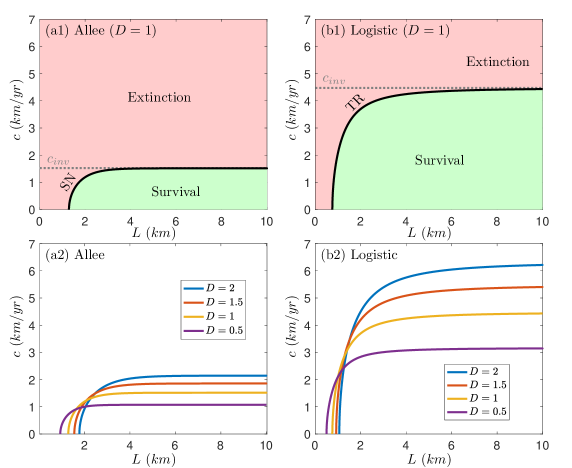
Figure 9: Two-parameter bifurcation diagrams for the RDE (2.1)–(2.2) in the parameter plane $(L,c)$ showing the boundary between the regions of (red) extinction and (green) survival, obtained by numerical continuation of SN and TR bifurcations of heteroclinic orbits in the compactified moving-frame ODE. The boundary is asymptotic to (the horizontal gray line) $c=c_{inv}$, where $c_{inv}$ depends on $D$; see section A.2 for details. (Left column) In the Allee model (4.2)–(4.3), the tipping boundary is a SN bifurcation of pulses. (Right column) In the logistic model (A.1)–(A.2), the boundary is a TR bifurcation of pulses. (Bottom row) The boundary for different values of $D$. Other parameter values are given in table 1.

4.5 Two-parameter bifurcation diagrams

In this section, we explore two-parameter bifurcation diagrams of pulse solutions in the habitat model (2.1)–(2.2). Primarily, we are interested in the persistence of stable carrying-capacity pulses when multiple parameters are varied. To start with, we compute the carrying-capacity pulse solution of the habitat model (2.1)–(2.2) as a heteroclinic orbit in the compactified system and detect a codimension-one bifurcation of this pulse solution while varying a single parameter. Then we trace this bifurcation as a one-dimensional curve in a two-parameter plane. In this way, we identify parameter regions of survival with a stable carrying-capacity pulse and extinction with the extinction state being the only stable state.

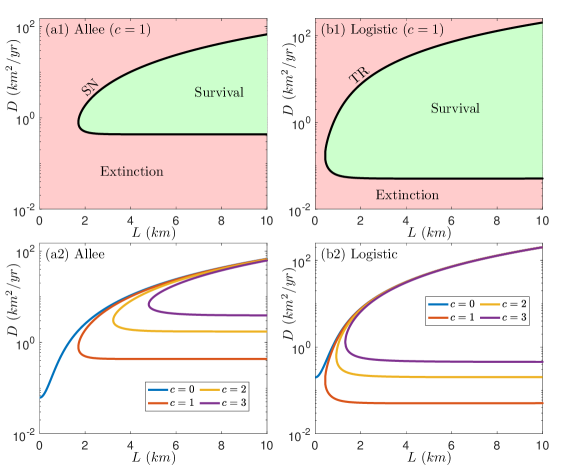
Figure 10: Two-parameter bifurcation diagrams for the RDE (2.1)–(2.2) in the parameter plane $(L,D)$ showing the boundary between the regions of (red) extinction and (green) survival, obtained by numerical continuation of SN and TR bifurcations of heteroclinic orbits in the compactified moving-frame ODE. See fig. 9 for more details.

The two-parameter bifurcation diagram in the ($L,c$)-plane for the Allee model (4.2)–(4.3) is shown in Figure 9(a1)–(a2). For $D=1$, the (red) extinction and (green) survival regions are separated by a (black) curve of SN bifurcations of pulse solutions; see Figure 9(a1). Note that SN has a (dotted grey) horizontal asymptote $c=c_{inv}$. In other words, no pulses can propagate faster than $c=c_{inv}$. It turns out that $c_{inv}$, often called the invasion speed, is the speed of a travelling front in an infinitely-long and homogeneous habitat. The separating tipping curves SN for different values of $D$ are shown in Figure 9(a2). As the dispersal rate $D$ is increased, the corresponding value of the invasion speed $c_{inv}$ (not displayed) also increases, and the survival region becomes larger.

For comparison, the two-parameter bifurcation diagram in the ($L,c$)-plane for the logistic growth model (A.1)–(A.2) is shown in Figure 9(b1)–(b2). The extinction and survival regions for $D=1$ are separated by a TR bifurcation of pulse solutions; see Figure 9(b1). The separating curves TR for different values of $D$ are shown in Figure 9(b2).

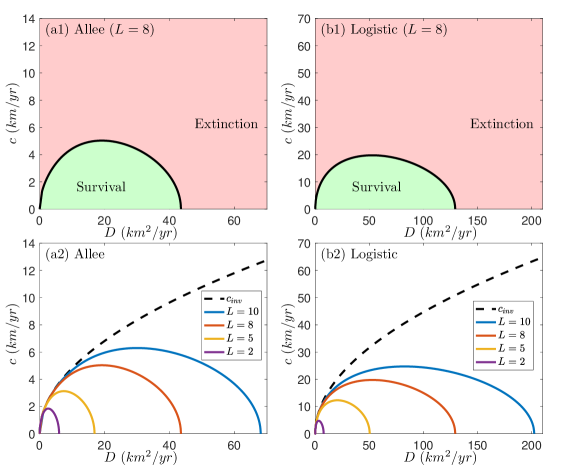
Figure 11: Two-parameter bifurcation diagrams for the RDE (2.1)–(2.2) in the parameter plane $(D,c)$ showing the boundary between the regions of (red) extinction and (green) survival, obtained by numerical continuation of SN and TR bifurcations of heteroclinic orbits in the compactified moving-frame ODE. See fig. 9 for more details.

The two-parameter bifurcation diagram of pulse solutions in the $(L,D)$-plane for the Allee growth model (4.2)–(4.3) is shown in Figure 10(a1)–(a2); note the logarithmic scale of $D$. For $c=1$, the tongue-shaped survival region is separated from extinction by a SN bifurcation of pulse solutions; see Figure 10(a1). For sufficiently large fixed $L$, survival is possible only within some bounded interval $(D_{min},D_{max})$ with $D_{min}>0$. When $0<D<D_{min}$, the dispersal rate is too low for the population to keep pace with the shifting habitat, and the habitat population falls below the Allee threshold, leading to extinction. When $D>D_{max}$, the large dispersal rate compels a larger proportion of the population to move outside the good habitat, causes the good habitat population to drop below the Allee threshold, and also leads to extinction. The observation that the population of moving habitats can only survive within a finite range of a dispersal rate has also been reported in [54]. The separating tipping curves SN for different values of $D$ are shown in Figure 10(a2). For $c>0$, the survival region of stable carrying-capacity travelling pulses sustain the tongue-like shape with $D_{min}>0$. However, for $c=0$, the survival region changes shape qualitatively so that it extends to $L=0$ and retains $D_{max}>0$, but $D_{min}$ becomes zero.

For comparison, the two-parameter bifurcation diagram of pulse solutions in the $(L,D)$-plane for the logistic growth model (A.1)–(A.2) is shown in Figure 10(b1)–(b2).

The two-parameter bifurcation diagram of pulse solutions in the $(D,c)$-plane for the Allee growth model (4.2)–(4.3) is shown in Figure 11(a1)–(a2). For $L=8$, the bubble-shaped survival region is separated from extinction by a SN bifurcation of pulse solutions; see Figure 11(a1). For sufficiently small fixed $c$, the survival region exists within a bounded interval $(D_{min},D_{max})$ with $D_{min}>0$ for reasons similar to those explained in the two paragraphs above. The separating tipping curves SN for different values of $L$ are shown in different colors in Figure 11(a2). When $L$ is increased, the survival region extends over a wider range in the $(D,c)$-plane. The different tipping curves accumulate on the dashed black curve, which shows the invasion speed $c_{inv}$ for an infinitely-long homogeneous good habitat $(L=\infty)$ as a function of the dispersal rate $D$.

For comparison, the two-parameter bifurcation diagram of pulse solutions in the $(D,c)$-plane for the logistic growth model (A.1)–(A.2) is shown in Figure 11(b1)–(b2).

5 Discussion

A brief overview of the article. Tipping points, or critical transitions, have been studied predominantly in ordinary differential equation (ODE) models. However, they remain largely unexplored in partial differential equation (PDE) models, where spatial dynamics can give rise to new tipping mechanisms. In this article, we studied tipping points in a special class of PDEs, namely, reaction-diffusion equations (RDEs) with a linearly time-varying and asymptotically-homogeneous reaction term. To analyze such problems, we introduced a mathematical framework that is based on two primary ingredients: (i) compactification of the moving-frame coordinate and (ii) computations of pulse and front solutions for such an RDE as heteroclinic orbits connecting two equilibria from infinity in the ensuing compactified ODE. As an illustrative example, we considered a conceptual ecosystem model subject to a geographically moving or shrinking habitat induced by climate change or human activity. Our focus was on tipping points to extinction for the population growth model with an Allee effect (cubic nonlinearity) and how it contrasts to the simpler logistic growth model (quadratic nonlinearity).

Summary of the framework. The summary of our framework is as follows. We started with a nondimensionalization of variables and parameters, followed by a reformulation of the nondimensionalized RDE into a first-order moving-frame ODE. Of importance is the fact that this ODE is only asymptotically autonomous. Thus, we applied a compactification technique, adapted from [66], to transform the nonautonomous ODE into an autonomous ODE on a suitably extended and compactified phase space that contains equilibria of autonomous limit systems from infinity. In the last step of the framework, we implemented a numerical method for obtaining pulse and front solutions for the RDE by computing heteroclinic orbits connecting these equilibria in the autonomous compactified ODE. Such heteroclinic orbits can be detected as intersections of the corresponding stable and unstable invariant manifolds using Lin’s method [39]. A particular advantage of our framework is that it also allows for numerical continuation of pulse and front solutions, as well as their bifurcations, in the space of the system and input parameters.

Summary of the example. To demonstrate its applicability, the mathematical framework was implemented in AUTO [14] and illustrated by the example of an ecosystem subject to a moving or shrinking habitat. As a result, we provided new insight into nonlinear dynamics of the moving habitat problem by performing the following:

• Computations of the two-dimensional unstable manifold of a hyperbolic saddle from negative infinity and the two-dimensional stable invariant manifold of a hyperbolic saddle from positive infinity in the compactified autonomous ODE.

• Computation of multiple heteroclinic orbits connecting these two saddles along intersections of the manifolds. These heteroclinic orbits correspond to coexisting pulse solutions for the ecosystem RDE, and may not be possible to obtain using traditional computational techniques.

• Continuation of these heteroclinic orbits to detect their bifurcations, which correspond to bifurcations of pulse solutions for the ecosystem RDE. We distinguished between dangerous bifurcations that give rise to tipping points (abrupt transitions to extinction) and safe bifurcations that give rise to gradual transitions to extinction

• Continuation of bifurcations of heteroclinic orbits for the compactified autonomous ODE to obtain two-parameter bifurcation diagrams of pulse solutions for the ecosystem RDE.

Our main findings include bifurcation-induced tipping (B-tipping) to extinction below some critical length of a shrinking habitat and rate-induced tipping (R-tipping) to extinction above some critical speed of a moving habitat. We also showed that abrupt tipping points found for the Allee growth model were replaced by gradual transitions to extinction for the logistic growth model. Finally, we examined the impact of system and input parameters by analyzing curves that separate regions of survival and extinction in two-parameter planes of: the habitat length and speed, the habitat length and population dispersion rate, and the population dispersion rate and habitat speed.

Future work. One interesting research direction for the future is to generalize the mathematical framework for tipping points in RDEs. Here, we considered reaction terms with linear time dependence, namely, $f(u,x-ct)$. Thus, we were able to simplify the original RDE to an ODE in the moving-frame coordinate $\xi=x-ct$. More generally, one will be interested in reaction terms with a nonlinear time dependence $g(rt)$, namely, $f(u,x-g(rt))$. However, such an RDE no longer simplifies to an ODE in the moving-frame coordinate $\xi=x-g(rt)$. Other interesting research directions include more complicated, possibly nonstationary, population dynamics within the habitat and extension to two spatial dimensions.

Funding

This work was supported by Laya Healthcare and the Enterprise Ireland Innovative Partnership Programme project IP20190771. CRH acknowledges the partial funding by the Natural Environment Research Council (grant NE/W005042/1). SW acknowledges partial support by the EvoGamesPlus Innovative Training Network funded by the European Union’s Horizon 2020 research and innovation program under the Marie Skłodowska-Curie grant agreement 955708.

Appendix A Appendix

A.1 Compactified logistic model

Here, we lay out the nondimensionalized compactified system for the logistic model

$$\left\{\begin{array}[]{rrl}\mathcal{U}_{z}&=&\mathcal{V},\\ \mathcal{V}_{z}&=&-\tilde{c}\,\mathcal{V}-\tilde{f}_{L}\Big{(}\mathcal{U},\tilde{H}_{\alpha}(s)\Big{)},\\ s_{z}&=&\dfrac{\alpha}{2}(1-s^{2}),\end{array}\right.$$ (A.1)

where the dimensionless logistic reaction term is expressed in terms of $s$ and given by

$$\tilde{f}_{L}\Big{(}\mathcal{U},\tilde{H}_{\alpha}(s)\Big{)}=\mathcal{U}\left(\tilde{\beta}^{2}\left(2\tilde{H}_{\alpha}(s)-1\right)-\mathcal{U}\right),$$ (A.2)

and the $s$-dependent habitat function, $\tilde{H}_{\alpha}(s)$, is given by (3.14) and (4.4).

A.2 Invasion speed in a homogeneous good habitat

Here, we compute the invasion speed in an infinite homogeneous habitat $(L=\infty$), which is the speed of travelling fronts for a constant $H(\xi)=1$. Thus, the reaction terms in the RDE (2.1) and the moving-frame ARDE (2.4) are now homogeneous and autonomous. In the nondimensionalized setting, this corresponds to setting $\tilde{H}(z)=1$ for all $z$, and the nonautonomous moving-frame ODE (3.5)–(3.6) is now autonomous. We obtain travelling fronts for the homogeneous RDE (2.1) by computing heteroclinic orbits in the autonomous moving-frame ODE (3.5)–(3.6).

A.2.1 Invasion speed in the Allee growth model

For the Allee model, we consider the ensuing autonomous system

$$\begin{split}\mathcal{U}_{z}&=\mathcal{V},\\ \mathcal{V}_{z}&=-\tilde{c}\,\mathcal{V}-\tilde{f}_{A}(\mathcal{U},1),\end{split}$$ (A.3)

with the Allee reaction term

$$\tilde{f}_{A}(\mathcal{U},1)=\mathcal{U}\left(-\tilde{\beta}^{2}+4\tilde{\beta}\,\mathcal{U}-\mathcal{U}^{2}\right).$$ (A.4)

System (A.3)–(A.4) has three equilibrium points,

$$\mathcal{U}^{*}_{0}:=(\mathcal{U},\mathcal{V})=(0,0),\quad\mathcal{U}^{*}_{1}:=(\mathcal{U},\mathcal{V})=((2-\sqrt{3})\tilde{\beta},0),\quad\mathcal{U}^{*}_{2}:=(\mathcal{U},\mathcal{V})=((2+\sqrt{3})\tilde{\beta},0),$$

which represent extinction, the Allee threshold, and carrying capacity, respectively. Stability analysis shows that $\mathcal{U}^{*}_{0}$ and $\mathcal{U}^{*}_{2}$ are always of saddle type. The Allee threshold equilibrium $\mathcal{U}^{*}_{1}$ is a center for $c=0$ and a sink for $c>0$. To find the speed $c=c_{inv}$ of travelling fronts, we seek a heteroclinic orbit that connects the saddle equilibria $\mathcal{U}^{*}_{0}$ and $\mathcal{U}^{*}_{2}$. We detect this heteroclinic orbit by computing the unstable manifold of $\mathcal{U}^{*}_{2}$ and the stable manifold of $\mathcal{U}^{*}_{0}$ and finding $c$ for which the two manifolds intersect; see Figure 12. In Figure 12(a)–(b), where $c<c_{inv}$ , the unstable manifold of $\mathcal{U}^{*}_{2}$ (red curve) lies below the stable manifold of $\mathcal{U}^{*}_{0}$ (blue curve). In Figure 12(c), where $c=c_{inv}$, the two manifolds intersect along a codimension-one heteroclinic orbit (magenta curve). In Figure 12(d), the unstable manifold of $\mathcal{U}^{*}_{2}$ (red curve) lies above the stable manifold of $\mathcal{U}^{*}_{0}$ (blue curve) and connects to saddle $\mathcal{U}^{*}_{1}$ instead. Since $c_{inv}$ depends on $D$, we use numerical continuation of heteroclinic orbits to obtain the invasion speed curve in the parameter plane $(D,c)$. We find that the invasion speed curve $c_{inv}$ indeed marks the upper bound for the speed of travelling pulses for a bi-asymptotically homogeneous habitat; see fig. 9(a1) and fig. 11(a2).

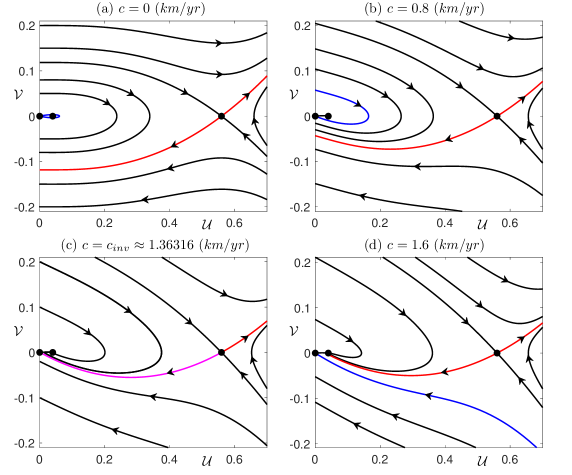
Figure 12: The phase portrait of system (A.3)–(A.4), (a)–(b) before, (c) at, and (d) after the heteroclinic orbit. Here, $D=0.8$ and $c$ is varied. From left to right, the black dots on the $V$-axis are the equilibria $\mathcal{U}^{*}_{0}$ (saddle), $\mathcal{U}^{*}_{1}$ (center for $c=0$ and sink for $c>0$), and $\mathcal{U}^{*}_{2}$ (saddle). The blue and red orbit trajectories represent the stable and unstable manifolds of $\mathcal{U}^{*}_{0}$ and $\mathcal{U}^{*}_{2}$, respectively. The magenta trajectory represents the heteroclinic orbit that connects $\mathcal{U}^{*}_{0}$ with $\mathcal{U}^{*}_{2}$ at $c=c_{inv}$.

A.2.2 Invasion speed in the logistic growth model

For the logistic model, the ensuing autonomous system is

$$\begin{split}\mathcal{U}_{z}&=\mathcal{V},\\ \mathcal{V}_{z}&=-\tilde{c}\,\mathcal{V}-\tilde{f}_{L}(\mathcal{U},1),\end{split}$$ (A.5)

with the logistic reaction term

$$\tilde{f}_{A}(\mathcal{U},1)=\mathcal{U}\left(\tilde{\beta}^{2}-\mathcal{U}\right).$$ (A.6)

System (A.5)–(A.6) has two equilibrium points,

$$\mathcal{U}^{*}_{0}:=(\mathcal{U},\mathcal{V})=(0,0),\quad\mathcal{U}^{*}_{1}:=(\mathcal{U},\mathcal{V})=(\tilde{\beta}^{2},0),$$

which represent extinction and the carrying capacity, respectively. Stability analysis shows that $\mathcal{U}^{*}_{0}$ is always a sink and $\mathcal{U}^{*}_{1}$ is always a saddle. The invasion speed can be obtained as follows; see, for example, [6, 8]. When $\tilde{c}^{2}<4\tilde{\beta}^{2}$, $\mathcal{U}^{*}_{0}$ is a stable spiral, and when $\tilde{c}^{2}\geq 4\tilde{\beta}^{2}$, $\mathcal{U}^{*}_{0}$ becomes a stable node. The heteroclinic orbit between $\mathcal{U}^{*}_{0}$ and $\mathcal{U}^{*}_{1}$ is of codimension-zero. However, when $\tilde{c}^{2}<4\tilde{\beta}^{2}$, this heteroclinic orbit crosses the $\mathcal{V}$-axis due to the spiralling nature of the spiral sink, which means that there is at least one negative $\mathcal{U}$-value along the heteroclinic orbit. On the other hand, when $\tilde{c}^{2}\geq 4\tilde{\beta}^{2}$, the heteroclinic orbit connecting $\mathcal{U}^{*}_{0}$ to $\mathcal{U}^{*}_{1}$ does not violate the condition $\mathcal{U}(z)\geq 0$ for all $z$. Therefore, the corresponding travelling front for $\tilde{c}^{2}\geq 4\tilde{\beta}^{2}$ is physically relevant if and only if $\tilde{c}^{2}\geq 4\tilde{\beta}^{2}$. Here, we define the invasion speed in the logistic model as the value of $c$ that corresponds to the onset of physically relevant travelling fronts. This onset is given by the analytical expression $\tilde{c}^{2}=4\tilde{\beta}^{2}$, or equivalently, $c=c_{inv}=2\sqrt{\beta D}$. We find that the invasion speed $c_{inv}$ indeed marks the upper bound for the speed of travelling pulses in the logistic model; see fig. 9(b1) and fig. 11(b2).

References

- [1] Hassan M Alkhayuon and Peter Ashwin. Rate-induced tipping from periodic attractors: Partial tipping and connecting orbits. Chaos: An Interdisciplinary Journal of Nonlinear Science, 28(3):033608, 2018.
- [2] Peter Ashwin, Clare Perryman, and Sebastian Wieczorek. Parameter shifts for nonautonomous systems in low dimension: bifurcation-and rate-induced tipping. Nonlinearity, 30(6):2185, 2017.
- [3] Peter Ashwin, Sebastian Wieczorek, Renato Vitolo, and Peter Cox. Tipping points in open systems: bifurcation, noise-induced and rate-dependent examples in the climate system. Philosophical Transactions of the Royal Society A: Mathematical, Physical and Engineering Sciences, 370(1962):1166–1184, 2012.
- [4] Golan Bel, Aric Hagberg, and Ehud Meron. Gradual regime shifts in spatially extended ecosystems. Theoretical Ecology, 5:591–604, 2012.
- [5] Henri Berestycki, Laurent Desvillettes, and Odo Diekmann. Can climate change lead to gap formation? Ecological Complexity, 20:264–270, 2014.
- [6] Henri Berestycki, Odo Diekmann, Cornelis J Nagelkerke, and Paul A Zegeling. Can a species keep pace with a shifting climate? Bulletin of mathematical biology, 71(2):399–429, 2009.
- [7] Juliette Bouhours and Thomas Giletti. Spreading and vanishing for a monostable reaction–diffusion equation with forced speed. Journal of dynamics and differential equations, 31(1):247–286, 2019.
- [8] José Canosa. On a nonlinear diffusion equation describing population growth. IBM Journal of Research and Development, 17(4):307–313, 1973.
- [9] Alan R Champneys. Homoclinic orbits in reversible systems and their applications in mechanics, fluids and optics. Physica D: Nonlinear Phenomena, 112(1-2):158–186, 1998.
- [10] Yuxin Chen, John A Gemmer, Mary Silber, and Alexandria Volkening. Noise-induced tipping under periodic forcing: Preferred tipping phase in a non-adiabatic forcing regime. Chaos: An Interdisciplinary Journal of Nonlinear Science, 29(4):043119, 2019.
- [11] Yuxin Chen, Theodore Kolokolnikov, Justin Tzou, and Chunyi Gai. Patterned vegetation, tipping points, and the rate of climate change. European Journal of Applied Mathematics, 26(6):945–958, 2015.
- [12] Brian Dennis. Allee effects: population growth, critical density, and the chance of extinction. Natural Resource Modeling, 3(4):481–538, 1989.
- [13] Eusebius J Doedel. Lecture notes on numerical analysis of nonlinear equations. In Numerical Continuation Methods for Dynamical Systems, pages 1–49. Springer, New York, 2007.
- [14] Eusebius J Doedel, Alan R Champneys, Fabio Dercole, Thomas F Fairgrieve, Yu A Kuznetsov, B Oldeman, RC Paffenroth, B Sandstede, XJ Wang, and CH Zhang. AUTO-07P: Continuation and Bifurcation Software for Ordinary Differential Equations, 2007, https://github.com/auto-07p.
- [15] Freddy Dumortier. Compactification and desingularization of spaces of polynomial Liénard equations. Journal of Differential Equations, 224(2):296–313, 2006.
- [16] Andrus Giraldo, Bernd Krauskopf, and Hinke M Osinga. Saddle invariant objects and their global manifolds in a neighborhood of a homoclinic flip bifurcation of case B. SIAM Journal on Applied Dynamical Systems, 16(1):640–686, 2017.
- [17] Andrus Giraldo, Bernd Krauskopf, and Hinke M Osinga. Cascades of global bifurcations and chaos near a homoclinic flip bifurcation: a case study. SIAM Journal on Applied Dynamical Systems, 17(4):2784–2829, 2018.
- [18] Andrus Giraldo, Bernd Krauskopf, and Hinke M Osinga. Computing connecting orbits to infinity associated with a homoclinic flip bifurcation. Journal of Computational Dynamics, 7(2):489–510, 2020.
- [19] Karna Gowda, Hermann Riecke, and Mary Silber. Transitions between patterned states in vegetation models for semiarid ecosystems. Physical Review E, 89(2):022701, 2014.
- [20] Aric Hagberg and Ehud Meron. Pattern formation in non-gradient reaction-diffusion systems: the effects of front bifurcations. Nonlinearity, 7(3):805–835, 1994.
- [21] Samir Hamdi, William E Schiesser, and Graham W Griffiths. Method of lines. Scholarpedia, 2(7):2859, 2007.
- [22] Melanie A Harsch, Austin Phillips, Ying Zhou, Margaret-Rose Leung, D Scott Rinnan, and Mark Kot. Moving forward: insights and applications of moving-habitat models for climate change ecology. Journal of ecology, 105(5):1169–1181, 2017.
- [23] James Alexander, Christopher KRT Jones and Robert Gardner. A topological invariant arising in the stability analysis of travelling waves. Journal für die reine und angewandte Mathematik, pages 167–212, 1990.
- [24] Christopher KRT Jones. Stability of the travelling wave solution of the Fitzhugh-Nagumo system. Transactions of the American Mathematical Society, 286(2):431–469, 1984.
- [25] Christopher KRT Jones. Instability of standing waves for nonlinear Schrödinger type equations. Ergodic Theory and Dynamical Systems, 8:119–128, 1988.
- [26] Christopher KRT Jones and Jerome V Moloney. Instability of standing waves in nonlinear optical waveguides. Physics Letters A, 117(4):175–180, 1986.
- [27] Todd Kapitula and Björn Sandstede. Eigenvalues and resonances using the Evans function. Discrete & Continuous Dynamical Systems, 10(4):857–869, 2004.
- [28] Michal Kozák, Eamonn A Gaffney, and Václav Klika. Pattern formation in reaction-diffusion systems with piecewise kinetic modulation: an example study of heterogeneous kinetics. Physical Review E, 100(4):042220, 2019.
- [29] Bernd Krauskopf. Bifurcations at in a model for 1: 4 resonance. Ergodic theory and dynamical systems, 17(4):899–931, 1997.
- [30] Bernd Krauskopf and Thorsten Rieß. A Lin’s method approach to finding and continuing heteroclinic connections involving periodic orbits. Nonlinearity, 21(8):1655, 2008.
- [31] Christian Kuehn. A mathematical framework for critical transitions: Bifurcations, fast–slow systems and stochastic dynamics. Physica D: Nonlinear Phenomena, 240(12):1020–1035, 2011.
- [32] Christian Kuehn. A mathematical framework for critical transitions: normal forms, variance and applications. Journal of Nonlinear Science, 23(3):457–510, 2013.
- [33] Christian Kuehn. PDE Dynamics: An Introduction, volume 23. SIAM, Philadelphia, 2019.
- [34] Yuri A Kuznetsov. Elements of applied bifurcation theory, volume 112. Springer Science, New York, 2013.
- [35] Uwe Langbein, Falk Lederer, and Hans-Ernst Ponath. Generalized dispersion relations for nonlinear slab-guided waves. Optics communications, 53(6):417–420, 1985.
- [36] Timothy M Lenton. Early warning of climate tipping points. Nature climate change, 1(4):201–209, 2011.
- [37] Timothy M Lenton, Johan Rockström, Owen Gaffney, Stefan Rahmstorf, Katherine Richardson, Will Steffen, and Hans Joachim Schellnhuber. Climate tipping points—too risky to bet against. Nature, 575:592–595, 2019.
- [38] Bingtuan Li, Sharon Bewick, Jin Shang, and William F Fagan. Persistence and spread of a species with a shifting habitat edge. SIAM Journal on Applied Mathematics, 74(5):1397–1417, 2014.
- [39] Xiao-Biao Lin. Using Melnikov’s method to solve Silnikov’s problems. Proceedings of the Royal Society of Edinburgh Section A: Mathematics, 116(3-4):295–325, 1990.
- [40] Quan-Xing Liu, Peter MJ Herman, Wolf M Mooij, Jef Huisman, Marten Scheffer, Han Olff, and Johan Van De Koppel. Pattern formation at multiple spatial scales drives the resilience of mussel bed ecosystems. Nature communications, 5(1):1–7, 2014.
- [41] Gabriel Andreguetto Maciel and Frithjof Lutscher. How individual movement response to habitat edges affects population persistence and spatial spread. The American Naturalist, 182(1):42–52, 2013.
- [42] Lawrence Markus. II. Asymptotically autonomous differential systems. In Contributions to the Theory of Nonlinear Oscillations (AM-36), volume 3. Princeton University Press Princeton, NJ, USA, 1956.
- [43] Kaname Matsue. On blow-up solutions of differential equations with Poincaré-type compactifications. SIAM Journal on Applied Dynamical Systems, 17(3):2249–2288, 2018.
- [44] José Mujica, Bernd Krauskopf, and Hinke M Osinga. A Lin’s method approach for detecting all canard orbits arising from a folded node. Journal of Computational Dynamics, 4(1&2):143–165, 2017.
- [45] Elle Musoke, Bernd Krauskopf, and Hinke M Osinga. A surface of heteroclinic connections between two saddle slow manifolds in the Olsen model. International Journal of Bifurcation and Chaos, 30(16):2030048, 2020.
- [46] Kei Nishi, Yasumasa Nishiura, and Takashi Teramoto. Dynamics of two interfaces in a hybrid system with jump-type heterogeneity. Japan journal of industrial and applied mathematics, 30(2):351–395, 2013.
- [47] Carlos Afonso Nobre and Laura De Simone Borma. “Tipping points” for the Amazon forest. Current Opinion in Environmental Sustainability, 1(1):28–36, 2009.
- [48] Paul E O’Keeffe and Sebastian Wieczorek. Tipping phenomena and points of no return in ecosystems: beyond classical bifurcations. SIAM Journal on Applied Dynamical Systems, 19(4):2371–2402, 2020.
- [49] Bart E Oldeman, Alan R Champneys, and Bernd Krauskopf. Homoclinic branch switching: A numerical implementation of Lin’s method. International Journal of Bifurcation and Chaos, 13(10):2977–2999, 2003.
- [50] Craig M Pease, Russell Lande, and JJ Bull. A model of population growth, dispersal and evolution in a changing environment. Ecology, 70(6):1657–1664, 1989.
- [51] Alex B Potapov and Mark A Lewis. Climate and competition: the effect of moving range boundaries on habitat invasibility. Bulletin of Mathematical Biology, 66(5):975–1008, 2004.
- [52] Paul Ritchie and Jan Sieber. Early-warning indicators for rate-induced tipping. Chaos: An Interdisciplinary Journal of Nonlinear Science, 26(9):093116, 2016.
- [53] Paul Ritchie and Jan Sieber. Probability of noise-and rate-induced tipping. Physical Review E, 95(5):052209, 2017.
- [54] Lionel Roques, Alain Roques, Henri Berestycki, and André Kretzschmar. A population facing climate change: joint influences of allee effects and environmental boundary geometry. Population Ecology, 50(2):215–225, 2008.
- [55] RD Russell and J Christiansen. Adaptive mesh selection strategies for solving boundary value problems. SIAM Journal on Numerical Analysis, 15(1):59–80, 1978.
- [56] Björn Sandstede. Stability of travelling waves. In Handbook of dynamical systems, volume 2, pages 983–1055. Elsevier, New York, 2002.
- [57] Björn Sandstede and Arnd Scheel. Essential instability of pulses and bifurcations to modulated travelling waves. Proceedings of the Royal Society of Edinburgh Section A: Mathematics, 129(6):1263–1290, 1999.
- [58] Marten Scheffer, Jordi Bascompte, William A Brock, Victor Brovkin, Stephen R Carpenter, Vasilis Dakos, Hermann Held, Egbert H Van Nes, Max Rietkerk, and George Sugihara. Early-warning signals for critical transitions. Nature, 461(7260):53–59, 2009.
- [59] Marten Scheffer, Steve Carpenter, Jonathan A Foley, Carl Folke, and Brian Walker. Catastrophic shifts in ecosystems. Nature, 413(6856):591–596, 2001.
- [60] Kimberly A Selkoe, Thorsten Blenckner, Margaret R Caldwell, Larry B Crowder, Ashley L Erickson, Timothy E Essington, James A Estes, Rod M Fujita, Benjamin S Halpern, Mary E Hunsicker, et al. Principles for managing marine ecosystems prone to tipping points. Ecosystem Health and Sustainability, 1(5):1–18, 2015.
- [61] John Michael T Thompson and Jan Sieber. Climate tipping as a noisy bifurcation: a predictive technique. IMA Journal of Applied Mathematics, 76(1):27–46, 2011.
- [62] Peter Van Heijster, Arjen Doelman, Tasso J Kaper, Yasumasa Nishiura, and Kei-Ichi Ueda. Pinned fronts in heterogeneous media of jump type. Nonlinearity, 24(1):127, 2010.
- [63] Egbert H Van Nes, Babak MS Arani, Arie Staal, Bregje van der Bolt, Bernardo M Flores, Sebastian Bathiany, and Marten Scheffer. What do you mean,“tipping point”? Trends in ecology & evolution, 31(12):902–904, 2016.
- [64] Vito Volterra. Population growth, equilibria, and extinction under specified breeding conditions: a development and extension of the theory of the logistic curve. Human Biology, 10(1):1–11, 1938.
- [65] Sebastian Wieczorek, Chun Xie, and Peter Ashwin. Rate-induced tipping: Thresholds, edge states and connecting orbits. Nonlinearity, 36(6):3238, 2023.
- [66] Sebastian Wieczorek, Chun Xie, and Chris KRT Jones. Compactification for asymptotically autonomous dynamical systems: theory, applications and invariant manifolds. Nonlinearity, 34(5):2970, 2021.
- [67] A Zafarullah. Application of the method of lines to parabolic partial differential equations with error estimates. Journal of the ACM, 17(2):294–302, 1970.
- [68] Yuval R Zelnik and Ehud Meron. Regime shifts by front dynamics. Ecological Indicators, 94:544–552, 2018.
- [69] Yuval R Zelnik, Ehud Meron, and Golan Bel. Gradual regime shifts in fairy circles. Proceedings of the National Academy of Sciences, 112(40):12327–12331, 2015.
- [70] Wenjun Zhang, Bernd Krauskopf, and Vivien Kirk. How to find a codimension-one heteroclinic cycle between two periodic orbits. Discrete & Continuous Dynamical Systems, 32(8):2825–2851, 2012.