Superiority in dense coding through non-Markovian stochasticity

Abstract

We investigate the distributed dense coding (DC) protocol, involving multiple senders and a single or two receivers under the influence of non-Markovian noise, acting on the encoded qubits transmitted from senders to the receiver(s). We compare the effects of non-Markovianity on DC both for the dephasing and depolarising channels. In the case of dephasing channels, we illustrate that for some classes of states, high non-Markovian strength can eradicate the negative influence of noisy channels which is not observed for depolarizing noise. Furthermore, we incorporate randomness into the noise models by replacing the Pauli matrices with random unitaries and demonstrate the constructive impact of stochastic noise models on the quenched averaged dense coding capacity. Interestingly, we report that the detrimental effect of non-Markovian depolarising channels in the DC protocol can be eliminated when randomness is added to the channel.

I Introduction

Entanglement, the nonlocal resource shared with distant partners, is the most inherent difference between a conventional classical information-sharing protocol and its quantum version Horodecki et al. (2009). Basic protocols like dense coding Bennett and Wiesner (1992), teleportation Bennett et al. (1993), key distribution Ekert (1991), and one-way quantum computation Raussendorf and Briegel (2001) take advantage of this salient feature to surpass the classical limit imposed by unentangled resource states. In particular, quantum dense coding (DC) is the process of transmitting classical information across a long distance using an entangled channel Bennett and Wiesner (1992). The key idea is to distribute an entangled state between the sender(s) and the receiver(s), with the senders first acting on their subsystems with local unitary operations before sending it to the receiver via a noiseless quantum channel Bose et al. (2000); Bowen (2001); Liu et al. (2002); Ziman and Bužek (2003a); Hiroshima (2001); Bruß et al. (2014, 2006); Laurenza et al. (2020). The receiver decodes the message by performing a joint measurement on the entire system. The successful implementation of the DC protocol consists of three steps - (i) encoding at the sender’s end, (ii) sending the encoded part through a channel connecting the sender and the receiver, and (iii) decoding the information via measurements at the receiver’s site. Moreover, the transmission of classical information has also been experimentally demonstrated over reasonably large separation of the parties with physical systems like photons Mattle et al. (1996); Shimizu et al. (1999); Mizuno et al. (2005); Pan et al. (2012); Northup and Blatt (2014); Barreiro et al. (2014); Krenn et al. (2016), and trapped ions Fang et al. (2000); Leibfried et al. (2003); Vandersypen and Chuang (2005); Yang and Gong (2007).

The dense coding capacity (DCC) of a shared resource state, which is characterized as the maximum amount of classical information that can be sent, is used to quantitatively assess the performance of the shared state in the DC protocol. It can be shown that not all entangled states are beneficial for DC Gross et al. (2009). In particular, a quantum state is said to be densecodeable if and only if it can provide a capacity greater than that achieved through purely classical means Hausladen et al. (1996); Bowen (2001); Horodecki et al. (2001). If the encoded parts are transmitted over a noiseless channel and the Holevo bound Holevo (1973, 1998) is used during the decoding of the information, the compact version of DCC can be determined analytically by maximizing over unitary encoding for any number of senders and a single receiver. When two receivers who can decode the message via local operations and classical communication (LOCC) are involved, the exact dense coding capacity is not known although the upper bound was provided Sen (De) by employing local Holevo-like bound Badzia¸g et al. (2003); Horodecki et al. (2004); Ghosh et al. (2005) which can be improved either by increasing the set of operations used for encoding Beran and Cohen (2008); Shadman et al. (2011, 2012) or through pre-processing Gupta et al. (2021). Port-based dense coding protocol Wu et al. (2006); Ji et al. (2006); Bourdon et al. (2008); Tsai and Hwang (2010); Srivastava et al. (2019) and probabilistic dense coding have also been addressed Hao et al. (2000); Feng et al. (2006); Kögler and Neves (2017).

Since isolated systems cannot be prepared, the systems under consideration are always in contact with the environment which, in general, is responsible for the decay of quantum properties like quantum correlations. Noise is often classified into two categories – Markovian noise Nielsen and Chuang (2000), which has no memory effect during evolution, and Non-Markovian noise Breuer and Petruccione (2007); Daffer et al. (2004); Rivas and Huelga (2012); Shrikant et al. (2018); Lidar (2019), which retains memories of earlier stages of the evolution and influences later noise processes. It was found that quantum correlations, by nature, are fragile against noise injected by the environment, e.g., under local dephasing noise, entanglement suddenly dies away – a phenomenon known as entanglement sudden death Yu and Eberly (2004); Dodd and Halliwell (2004); Ficek and Tanaś (2006); Almeida et al. (2007); Yu and Eberly (2009); Mazzola et al. (2009) which, in turn, affects all the information processing tasks. Specifically, the DC protocol can be affected by noise in two ways – first, when sharing the resource state, which has already been considered in the derivation of DCC Bose et al. (2000); Bowen (2001); Horodecki et al. (2001); Ziman and Bužek (2003b); Bruß et al. (2014, 2006) and second, when sending to the receiver(s) for which DCC affected by certain kinds of Markovian noise has also been addressed Quek et al. (2010); Shadman et al. (2010, 2011, 2012, 2013); Das et al. (2014, 2015); Mirmasoudi and Ahadpour (2018)(cf. Liu et al. (2016) for non-Markovian noise with a single sender-receiver pair).

In this work, we examine the impact of both Markovian and Non-Markovian noises on the dense coding protocol involving multiple senders and one or two receivers. Our aim is to determine whether the non-Markovian nature of the noise, has any favorable impact on the transmission of classical information, an effect which was already observed in the instance of correlation measures Mazzola et al. (2009); Rivas et al. (2010); Mazzola et al. (2010); Haikka et al. (2013); Lo Franco and Compagno (2017); Karpat et al. (2017); Gupta et al. (2022). Specifically, we demonstrate that when the shared states are the generalized Greenberger-Horne-Zeilinger (gGHZ) Greenberger et al. (2007); Yimsiriwattana and Lomonaco (2004) and generalized W states (gW) Dür et al. (2000); Sen (De), the DCC can be enhanced in the presence of high dephasing noise and high non-Markovianity compared to Markovian dephasing noise, thereby eliminating the detrimental effects of noise on the protocol. Interestingly, we observe that for depolarizing non-Markovian noise, such an increment is absent. Furthermore, compared to the DC protocol with more senders, the increase of DCC under non-Markovian noise is more pronounced in the three-party case, involving only two or three senders. It might demonstrate how the advantage is determined by the trade-off between noise and the non-Markovianity parameter of the channel.

On a different front, the inherently stochastic nature of quantum theory allows for the existence of randomness which is a thriving area of research in the context of random unitaries and circuits. Various studies have been devoted to the dynamics of entanglement involving the properties of many-body systems Chan et al. (2018); von Keyserlingk et al. (2018), to demonstrate operator spreading Nahum et al. (2018), and random unitaries Nahum et al. (2017); Zhou and Nahum (2019); Li et al. (2022). It is quite unnatural to anticipate that the noise affecting resources will be of a specific sort, such as dephasing or depolarizing noise. Instead, a certain type of noise with some fluctuations that can be represented by random unitaries selected from a Gaussian distribution with a fixed standard deviation around the Pauli matrix, can replicate a more realistic environment. We perform quenched averaging of DCC over several such realizations. We manifest that for a fixed amount of non-Markovianity, the quenched averaged DCC and its upper bound for two receivers increase with the increase of disorder strength when the shared states are the gGHZ and the gW. Specifically, we highlight the advantages of the averaged DCC achieved under random non-Markovian depolarizing noise over the same without any disorder.

Our paper is arranged in the following manner. In Sec. II, the dense coding capacity with a single and two receivers are discussed along with the non-Markovian and random noise models. We also define certain quantities required for in-depth analysis of the noisy dense coding protocol in the same section. The positive impact of non-Markovianity on DCC is presented in Sec. III while Sec. IV demonstrates DCC under the random noise models. Finally, we summarise our observations in Sec. V.

II Prerequisites

We lay down the framework required for the analysis of our findings in this section. Starting with a brief outline of the dense coding protocol involving an arbitrary number of senders and a single as well as two receivers, we discuss how to construct random non-Markovian channels. We also define quantities that capture the critical behavior of the noise strength for obtaining quantum advantage.

II.1 Noisy Dense Coding Capacity

The dense coding capacity (DCC) quantifies the amount of classical information that can be transmitted with the help of a shared quantum state, known as the resource state. A second quantum channel is also required, through which the senders transfer their qubits to the receiver(s) after encoding the message. When the second channel is noiseless, the DCC for an $(N+1)$-qubit state, $\rho_{\mathcal{S}_{1}...\mathcal{S}_{N}\mathcal{R}}$, shared between $N$ senders, $\mathcal{S}_{i}$ $(i=1,2,3,\dots,N)$ and a single receiver, $\mathcal{R}$, reads Bruß et al. (2014, 2006)

$$C^{1}(\rho_{\mathcal{S}_{1}...\mathcal{S}_{N}\mathcal{R}})=\text{max} [\log_{2}d_{\mathcal{S}_{1}...\mathcal{S}_{N}},\log_{2}d_{\mathcal{S}_{1}...\mathcal{S}_{N}}+$$ (1)

$$S(\rho_{\mathcal{R}})-S(\rho_{\mathcal{S}_{1}...\mathcal{S}_{N}\mathcal{R}})].$$

Here, $\log_{2}d_{\mathcal{S}_{1}\dots\mathcal{S}_{N}}=\log_{2}d_{\mathcal{S}_{1}}d_{\mathcal{S}_{2}}\dots d_{\mathcal{S}_{N}}$ corresponds to the capacity without quantum advantage, referred to as the classical bound, with $d_{\mathcal{S}_{i}}(i=1,2,\dots,N)$ being the dimension of the subsystem of the sender, $\mathcal{S}_{i}$. $S(\rho)=-\text{Tr}(\rho\log_{2}\rho)$ is the von-Neumann entropy and $\rho_{\mathcal{R}}$ is the reduced subsystem at the receiver’s end, obtained by tracing out the senders’ part of the original state, i.e., $\rho_{\mathcal{R}}=\text{Tr}_{\mathcal{S}_{1}...\mathcal{S}_{N}}\rho_{\mathcal{S}_{1}...\mathcal{S}_{N}\mathcal{R}}$. A resource state is said to be densecodeable when $S(\rho_{\mathcal{R}})-S(\rho_{\mathcal{S}_{1}...\mathcal{S}_{N}\mathcal{R}})>0$, signifying quantum advantage over the classical bound. Note that Eq. (1) is obtained by considering that the encoding performed by the senders is through unitary operations (cf. Horodecki and Piani (2012)). We refer to this protocol as $N\mathcal{S}-1\mathcal{R}$.

When the channel through which the senders transmit their qubits to the receiver is noisy, the multipartite DCC has been shown to be Shadman et al. (2010)

$$C^{1}_{\text{noise}}(\rho_{\mathcal{S}_{1}...\mathcal{S}_{N}\mathcal{R}})=\text{max} [\log_{2}d_{\mathcal{S}_{1}...\mathcal{S}_{N}},\log_{2}d_{\mathcal{S}_{1}...\mathcal{S}_{N}}+$$ (2)

$$S(\rho_{R})-S(\tilde{\rho})],$$

where

$$\tilde{\rho}=\Lambda( (U^{\min}_{\mathcal{S}_{1}}\otimes...\otimes U^{\min}_{\mathcal{S}_{N}}\otimes\mathbb{I}_{\mathcal{R}})\rho_{\mathcal{S}_{1}...\mathcal{S}_{N}\mathcal{R}}$$ (3)

$$(U^{\dagger min}_{\mathcal{S}_{1}}\otimes...\otimes U^{\dagger min}_{\mathcal{S}_{N}}\otimes\mathbb{I}_{\mathcal{R}})).$$

Here $\Lambda$ is a completely positive trace preserving (CPTP) map denoting the noisy channel and $U^{\min}_{\mathcal{S}_{i}}$, a local unitary applied by the sender $i$, such that the von-Neumann entropy in the last term of Eq. (2) is minimized. If the noisy channel $\Lambda$ is covariant which means that it commutes with a complete set of orthogonal unitary operators, $\{W_{i}\}$ Shadman et al. (2010, 2013), we have

$$\Lambda(W_{i}\rho W^{\dagger}_{i})=W_{i}\Lambda(\rho)W^{\dagger}_{i}.$$ (4)

The noisy dense coding capacity with covariant noise reduces to Shadman et al. (2010)

$$C^{1}_{\text{noise}}(\rho_{\mathcal{S}_{1}...\mathcal{S}_{N}\mathcal{R}})=\text{max} [\log_{2}d_{\mathcal{S}_{1}...\mathcal{S}_{N}},\log_{2}d_{\mathcal{S}_{1}...\mathcal{S}_{N}}+$$ (5)

$$S(\rho_{\mathcal{R}})-S(\Lambda(\rho))].$$

Note that the simplification occurs since the noisy channel $\Lambda$, commutes with the entropy minimizing unitaries $U^{\min}_{\mathcal{S}_{i}}$ and the von-Neumann entropy remains unchanged upon the action of local unitary operators. A paradigmatic example of such a channel is the depolarising channel given in Eq. (LABEL:eq:depo_channel), while the dephasing channel is not so. Thus, in order to estimate the DCC of a resource state in the presence of a noisy channel that is not covariant, the minimization over the unitaries $U^{\min}_{\mathcal{S}_{i}}$ has to be performed. In this work, we will consider that the senders’ nodes are affected individually by both the dephasing and depolarising noise, after encoding.

Distributed Super Dense Coding Capacity in a noisy environment

Let us consider that the state, $\rho_{\mathcal{S}_{1}...\mathcal{S}_{N}\mathcal{R}_{1}\mathcal{R}_{2}}$, is shared between $N$ senders and two receivers such that the first $r$ senders, $\mathcal{S}_{1},...,\mathcal{S}_{r}$, communicate their classical message to $\mathcal{R}_{1}$, while the remaining senders, $\mathcal{S}_{r+1},...,\mathcal{S}_{N}$, do so to $\mathcal{R}_{2}$. Local operations and classical communication (LOCC) between two receivers are allowed for decoding, and we call this scheme $N\mathcal{S}-2\mathcal{R}$. Instead of Holevo bound Holevo (1973) which is used to derive DCC for a single receiver, Holevo-like bound for LOCC Badzia¸g et al. (2003) can be applied to obtain distributed DCC. Since it is known that this bound can be achieved asymptotically, we obtain only the upper bound on the dense coding capacity which reads as Bruß et al. (2006)

$$B^{2}(\rho_{\mathcal{S}_{1}...\mathcal{S}_{N}\mathcal{R}_{1}\mathcal{R}_{2}} )=\text{max}[\log_{2}d_{\mathcal{S}_{1}...\mathcal{S}_{N}},\log_{2}d_{\mathcal{S}_{1}...\mathcal{S}_{N}}+$$ (6)

$$S(\rho_{\mathcal{R}_{1}})+S(\rho_{\mathcal{R}_{2}})-\text{max}_{\begin{subarray}{c}x=1,2\end{subarray}}S(\xi^{x})],~{}~{}~{}~{}~{}~{}$$

where $\rho_{R_{i}}$ is the subsystem of the receiver $i(i=1,2)$, obtained by tracing out all the senders and the other receiver. Here, $\xi^{1}=\text{Tr}_{\mathcal{S}_{r+1}..\mathcal{S}_{N}\mathcal{R}_{2}}\rho_{\mathcal{S}_{1}...\mathcal{S}_{N}\mathcal{R}_{1}\mathcal{R}_{2}}$,     and $\xi^{2}=\text{Tr}_{\mathcal{S}_{1}..\mathcal{S}_{r}\mathcal{R}_{1}}\rho_{\mathcal{S}_{1}...\mathcal{S}_{N}\mathcal{R}_{1}\mathcal{R}_{2}}$, where the former is obtained by tracing out the second group of senders $(\mathcal{S}_{r+1},\dots,\mathcal{S}_{N})$ and a receiver $\mathcal{R}_{2}$. Similarly, we obtain $\xi^{2}$. Let us now suppose that the channels through which the two sets of senders transfer their qubits to the respective receivers are noisy, represented by $\Lambda$. The upper bound on the DCC alters as Das et al. (2015)

$$B^{2}_{\text{noise}}(\rho_{\mathcal{S}_{1}...\mathcal{S}_{N}\mathcal{R}_{1}\mathcal{R}_{2}} )=\text{max}[\log_{2}d_{\mathcal{S}_{1}...\mathcal{S}_{N}},\log_{2}d_{\mathcal{S}_{1}...\mathcal{S}_{N}}$$

$$+S(\rho_{\mathcal{R}_{1}})+S(\rho_{\mathcal{R}_{2}})-\text{max}_{\begin{subarray}{c}x=1,2\end{subarray}}S(\tilde{\xi}^{x})].$$

Here, $\tilde{\xi}^{x}$ again represents the reduced subsystems of the corresponding senders-receiver pairs as

$$\tilde{\xi}^{1}=$$

$$\text{Tr}_{\mathcal{S}_{r+1}..\mathcal{S}_{N}\mathcal{R}_{2}}\Lambda( (U^{\min}_{\mathcal{S}_{1}}\otimes...\otimes U^{\min}_{\mathcal{S}_{N}}\otimes\mathbb{I}_{\mathcal{R}_{1}\mathcal{R}_{2}})\rho_{\mathcal{S}_{1}...\mathcal{S}_{N}\mathcal{R}_{1}\mathcal{R}_{2}}\times$$

$$(U^{\dagger min}_{\mathcal{S}_{1}}\otimes...\otimes U^{\dagger min}_{\mathcal{S}_{N}}\otimes\mathbb{I}_{\mathcal{R}_{1}\mathcal{R}_{2}})),$$

and similarly $\tilde{\xi}^{2}$. Like in the single receiver scenario, local unitaries $U^{\min}_{\mathcal{S}_{i}}$s are applied in order to minimize the entropy in the last term of Eq. (LABEL:eq:DCC_2R_noisy). Note that $U^{\min}_{\mathcal{S}_{1}}\otimes...\otimes U^{\min}_{\mathcal{S}_{r}}$ and $U^{\min}_{\mathcal{S}_{r+1}}\otimes...\otimes U^{\min}_{\mathcal{S}_{N}}$ independently minimize $S(\tilde{\xi}^{1})$ and $S(\tilde{\xi}^{2})$ respectively. As in Eq. (5), the covariant channels lead to a capacity similar to Eq. (LABEL:eq:DCC_2R_noisy), with a modification in $\tilde{\xi}^{x}$.

II.2 Action of random quantum channels

Exemplary noise models considered typically in the literature include the dephasing, depolarising, amplitude damping channels Preskill (2018) (see Appendix A for Kraus representation of the dephasing and depolarizing channels). However, in reality, they can seldom be realized accurately according to their Kraus representation involving the Pauli matrices. During the dense coding protocol, the noise acting on the encoded qubits at the senders’ side may be quite different from the Pauli noise that characterizes some channels like dephasing and depolarizing. To address such a situation, local noise models based on random unitary operators are considered, representing the noise that actually affects each qubit sent to the receiver(s). An arbitrary two-dimensional unitary matrix $U$ is parameterized by four variables as

$$U=e^{i\phi}\begin{pmatrix}e^{i\omega/2}&0\\ 0&e^{-i\omega/2}\end{pmatrix}\begin{pmatrix}\cos\theta/2&-\sin\theta/2\\ \sin\theta/2&\cos\theta/2\end{pmatrix}\begin{pmatrix}e^{i\delta}&0\\ 0&e^{-i\delta}\end{pmatrix}.$$ (9)

For brevity, we set $\phi=0$, since it only contributes to an overall phase. Here, specific values of $\omega$, $\theta$, and $\delta$ lead to the well-known Pauli matrices. The values of the remaining three parameters which characterize the Pauli matrices (up to a global phase) are given by $\sigma_{x}:\omega=2\pi,\theta=\pi,\delta=\pi$; $\sigma_{y}:\omega=3\pi,\theta=\pi,\delta=\pi$; and $\sigma_{z}:\omega=2\pi,\theta=0,\delta=3\pi$. Note that the values of $\omega,\theta$, and $\delta$, mentioned above, are not unique for a given Pauli matrix. We design the random noisy channels by replacing $\sigma_{i}$s in Eqs. (A) and (LABEL:eq:depo_channel) by random unitary matrices given in Eq. (9). The parameters of the random unitary $U_{i}$ corresponding to a given $\sigma_{i}(i=x,y,z)$ are chosen from a Gaussian distribution with the corresponding mean, $\mu$ and a fixed standard deviation, say $\epsilon$, denoted by $\mathbb{G}(\mu,\epsilon)$. For example, the random unitary $U_{x}$ corresponding to $\sigma_{x}$ has its parameters $\omega,\theta$, and $\delta$ chosen from Gaussian distributions, $\mathbb{G}(2\pi,\epsilon),\mathbb{G}(\pi,\epsilon)$ and $\mathbb{G}(\pi,\epsilon)$ respectively, which in turn, quantifies the fluctuation around $\sigma_{x}$ during implementation. Hence, we can redefine the Kraus operators for the random non-Markovian dephasing and depolarising channels respectively as

$$\kappa_{I}^{dph}=\sqrt{[1-\alpha p](1-p)}\mathbb{I},\kappa_{z}^{dph}=\sqrt{[1+\alpha(1-p)]p}U_{z},$$

with $0\leq p\leq 1/2$ and

$$\kappa_{I}^{dp}=\sqrt{[1-3\alpha p](1-p)}\mathbb{I},\kappa_{i}^{dp}=\sqrt{\frac{[1+3\alpha(1-p)]p}{3}}U_{i},$$

(10)

with $i=x,y$ and $z$, $\alpha$ denotes the strength of the non-Markovianity with $0\leq\alpha\leq 1$ ($\alpha=0$ indicates the Markovian scenario) and $p$ ($0\leq p\leq 1/3\alpha$) is the strength of the noise. Note that, unlike the dephasing channel, the depolarising one is covariant even in the presence of non-Markovianity. However, even a small deviation from the usual Pauli matrices makes the channel incovariant. Below, we estimate $U^{\min}$ which is required to optimize the DCC in the presence of dephasing noise for a class of shared states.

Theorem 1. For the dense coding protocol involving $N$ senders and a single receiver sharing an $(N+1)$- qubit gGHZ state affected by local dephasing noise, the optimizing unitaries $U^{\min}$ corresponding to each sender are proportional to the identity operator.

Proof. The $(N+1)$- qubit gGHZ state is given by $|gGHZ\rangle^{N+1}=x|0\rangle^{\otimes N+1}+\sqrt{1-x^{2}}|1\rangle^{\otimes N+1}$. The only term in its DCC, given by Eq. (2), that involves the noisy channel and the minimizing unitaries is $S(\Lambda(\tilde{\rho}_{gGHZ}))$. For each sender, $\mathcal{S}_{j}$, the unitary $U^{\min}_{\mathcal{S}_{j}}$ can be parameterized (up to an overall phase) by $\omega_{j},\theta_{j}$, and $\delta_{j}$ as discussed in Eq. (9). Under the influence of the local dephasing channel, each of the non-zero eigenvalues of $\Lambda(\tilde{\rho}_{gGHZ})$ have the functional form as

$$\exp[i\sum_{j=1}^{N-1}(\omega_{j}+\delta_{j})]\sqrt{\exp[-2i\sum_{j=1}^{N-1}(\omega_{j}+\delta_{j})]f(x,\alpha,p,\theta_{j})},$$ (11)

where the function $f$ contains the dependence on the state parameter $x$, the noise parameters $\alpha$ and $p$, and the unitary parameters $\theta_{j}$. Evidently, the eigenvalues are independent of $\omega_{j}$ and $\delta_{j}$ and thus the entropy term depends only on $\theta_{j}$ of each $U^{\min}_{\mathcal{S}_{j}}$. Minimizing $S(\Lambda(\tilde{\rho}_{gGHZ}))$ with respect to $\theta_{j}$, yields the optimal value $\theta_{j_{\text{opt}}}\approx n\pi$. Thus, $\cos\theta_{j}\approx\pm 1$ and $\sin\theta_{j}\approx 0$ which implies $U^{\min}_{\mathcal{S}_{j}}\propto\mathbb{I}$ (where $\mathbb{I}$ is the $2\times 2$ identity operator). Hence the proof. $\hfill\blacksquare$
Remark. Note that if the shared state is an arbitrary $N$-qubit state, $U^{\min}$ may not simplify to the identity operator.

II.3 Critical noise strengths

Let us define certain physical quantities which can help us to analyze the effect of noise on the DCC. These quantities are introduced from the overall behavior that emerges in the DC protocol due to decoherence along with imperfections. In the presence of noise, one can expect the following changes in any indicator $\mathcal{Q}$ quantifying the protocol’s performance, which is the dense coding capacity in this case.

1. Typically, $\mathcal{Q}$ decreases with the increase of the noise strength $p$ and vanishes either at a finite $p$ or asymptotically. Hence, we define the minimum value of the noise strength, referred to be a critical noise strength, denoted by $p_{c}$, at which the DCC or quenched averaged DCC (which will be defined later for random noise) collapses to its classical limit for a fixed value of $\alpha$ as

   $$p_{c}=\min_{p}[p|C^{1}_{\text{noise}}~{}\text{or}~{}B^{2}_{\text{noise}}=\log_{2}(d_{\mathcal{S}_{1}}\dots d_{\mathcal{S}_{N}})].$$ (12)

   A lower value of $p_{c}$ indicates that the state involved in the protocol is more susceptible to noise and vice versa.

2. In presence of non-Markovian noise, $\mathcal{Q}$, in general, revives after collapse due to the backflow of information. For example, we know that it is the case for entanglement Rivas et al. (2010); Lo Franco and Compagno (2017); Karpat et al. (2017); Gupta et al. (2022). Motivated by this picture, the minimum value of $p$, at which the capacity first goes beyond its classical limit after collapse can be called the revival strength of noise - denoted by $p_{r}$, given by

   $$p_{r}=\min_{p}[p\geq p_{c}|C^{1}_{\text{noise}}~{}\text{or}~{}B^{2}_{\text{noise}}>\log_{2}(d_{\mathcal{S}_{1}}\dots d_{\mathcal{S}_{N}})].$$ (13)

   The constructive effect of the noise, if induced, is more prominent when the value of $p_{r}$ is low which indicates that the capacity revives faster.

3. Moreover, it is possible to identify a range of the noise parameter, in which non-Markovianity helps to overcome the detrimental effect that occurred due to Markovian noise, thereby illustrating the constructive effect of non-Markovianity. To compare the Markovian and non-Markovian noise scenarios, we define the quantity manifesting the advantage furnished by non-Markovianity, denoted by $p_{a}$, as

   $$p_{a}=\min_{p}[p| C^{1}_{\text{noise}}(\alpha>0)~{}>C^{1}_{\text{noise}}(\alpha=0)~{}$$ (14)

   $$\text{or}~{}~{}B^{2}_{\text{noise}}(\alpha>0)>B^{2}_{\text{noise}}(\alpha=0)].$$

We will investigate the patterns of the above quantities depending on the noise models and shared resource states in the succeeding sections. Note, however, that typically, to obtain a quantum advantage in the dense coding protocol, a high amount of entanglement is required and so it is not apriori guaranteed that the feature of revival that is observed for entanglement Gupta et al. (2022), can also be apparent for DCC. The above quantities $p_{c},p_{r}$, and $p_{a}$ highlight the different impacts of noise on the dense coding protocol.

III Dense Coding influenced by Non-Markovian noise

We investigate the response of non-Markovian dephasing and depolarising noise on the dense coding scheme. The noise acts on each channel that carries the encoded qubits from the senders’ side to the receiver(s). Specifically, we aim to find out whether non-Markovian noise in the channel can have a constructive impact on the capacity or not. If yes, we are interested to identify a range of parameters in the channel where such an effect is predominant.

Before going to a protocol with an arbitrary number of senders and a single or two receivers, let us consider the simplest bipartite scenario involving a single sender and a single receiver. One can check that $C^{1}_{\text{noise}}(\alpha>0)>C^{1}_{\text{noise}}(\alpha=0)$ for high values of the noise parameter, $p$, and the non-Markovianity strength $\alpha$, when the shared state is $|\phi^{+}\rangle_{\mathcal{S}\mathcal{R}}$ (see Appendix. B). It will be interesting to find whether such an advantage persists for arbitrary shared multipartite states in the $N$ senders - $1$ receiver and $N$ senders - $2$ receivers regimes. In this respect, note that it was shown that the relation between multipartite entanglement and DCC differs from the bipartite domain Das et al. (2015) and hence the effects of noise observed in the case of DCC with two parties may not hold in the multipartite domain which is indeed the case as shown in the succeeding sections.

III.1 Noisy dense coding between arbitrary senders and a single receiver

In the multipartite domain, a natural choice of the resource state is an $(N+1)$-party generalized GHZ (gGHZ) state, given by $|gGHZ\rangle^{N+1}=x|0\rangle^{\otimes N+1}+\sqrt{1-x^{2}}|1\rangle^{\otimes N+1}$, shared between $N$ senders and a single receiver. Such a choice is due to the fact that in the noiseless scenario, $|gGHZ\rangle^{N+1}$ with $x=\sqrt{1/2}$ provides the maximum DCC, i.e., $\log_{2}d_{\mathcal{S}_{1}}\dots d_{\mathcal{S}_{N}}+1$ while for other values of $x$, the capacity reads as $\log_{2}d_{\mathcal{S}_{1}}\dots d_{\mathcal{S}_{N}}+H(\{x^{2},1-x^{2}\})$ where $H(\{p_{i}\})=-\sum_{i}p_{i}\log_{2}p_{i}$ represents the Shannon entropy corresponding to the single-site reduced density matrix at the receiver’s end having eigenvalues, $\{x^{2},1-x^{2}\}$.

Impacts of dephasing non-Markovian channel. In the presence of both Markovian and non-Markovian noise $(\alpha\neq 0)$, the dephasing channel is not covariant, which implies that the minimization over $U^{\min}$ corresponding to each of the $N$ senders has to be performed. However, such optimization is hard to perform analytically and so we will resort to numerical optimization in obtaining the exact trends of the DCC by varying the noise parameter and the strength of non-Markovianity.

Before proceeding further, we present a lower bound on the DCC in the presence of the non-Markovian dephasing channel.
Theorem 2. The lower bound on the DCC, obtained under the non-Markovian dephasing channel, provides an advantage over its Markovian counterpart, for a certain range of the noise parameter when an $(N+1)$- qubit gGHZ state is shared between $N$ senders and a single receiver.

Proof. As stated before, the DCC without noise for the shared gGHZ state, $|gGHZ\rangle^{N+1}$, with $N$ senders and a single receiver can be obtained. In the presence of noise, motivated by Theorem 1., let us assume that $U^{\min}=\mathbb{I}_{\mathcal{S}_{1}}\otimes\mathbb{I}_{\mathcal{S}_{2}}\otimes\dots\otimes\mathbb{I}_{\mathcal{S}_{N}}$ (with $\mathbb{I}$ being the $2\times 2$ identity matrix), which leads to a lower bound on the actual DCC. In this case, the capacity reduces to $C^{1}_{\text{noise}}=\log_{2}d_{\mathcal{S}_{1}}\dots d_{\mathcal{S}_{N}}+H(\{x^{2},1-x^{2}\})-S(\Lambda(\rho^{N+1}))$ where $\rho^{N+1}=|gGHZ\rangle^{N+1}\langle gGHZ|$ with $\Lambda$ being the non-Markovian dephasing channel. Notice first, that under the action of the dephasing channel (both Markovian and non-Markovian), the coefficients in the density matrix only get modified but no additional coefficients appear beyond those of the pure state. This implies that there are only two eigenvalues, given by

$$\frac{1}{2}\Big{(}1\pm\sqrt{1-4(-1+(1-2p)^{2N})x^{2}(x^{2}-1)}\Big{)},~{}~{}\text{and}$$

$$\frac{1}{2}\Big{(}1\pm\sqrt{1-4(-1+(1-2p+2(p-1)p\alpha)^{2N})x^{2}(x^{2}-1)}\Big{)},$$

(15)

for the Markovian and non-Markovian channels respectively. Since both $S(\rho_{\mathcal{R}})$ and $S(\Lambda(\rho^{N+1}))$ are bi-variate functions, it is clear that the state is dense codeable when the smaller eigenvalue of $S(\Lambda(\rho^{N+1}))$ is lower than that of $S(\rho_{\mathcal{R}})$, thereby making $S(\rho_{\mathcal{R}})\geq S(\Lambda(\rho^{N+1}))$. Let us consider that the eigenvalues of $\rho_{\mathcal{R}}$ are such that $x^{2}<(1-x^{2})$. In the case of the Markovian channel, it is observed that the lower eigenvalue is less than $x^{2}$, when $p\leq 1/2$. Thus for the Markovian dephasing channel, the gGHZ state always gives a quantum advantage in the dense coding protocol.
Repeating the same exercise with the lower eigenvalue in Eq. (15), we find that the non-Markovian dephasing noise allows for dense codeability of the gGHZ state when $p\neq p_{c}=(1+\alpha-\sqrt{1+\alpha^{2}})/2\alpha$, which is the noise strength at which the capacity reduces to its classical limit. Thus a higher value of $\alpha$ decreases the noise strength at which the state ceases to be dense codeable. However, comparing $S(\Lambda_{M}(\rho^{N+1}))$ and $S(\Lambda_{NM}(\rho^{N+1}))$, with the subscript being the types of noise in the channel, we find that when $p\geq p_{a}=(2+\alpha-\sqrt{4+\alpha^{2}})/2\alpha$, $S(\Lambda_{M}(\rho^{N+1}))\geq S(\Lambda_{NM}(\rho^{N+1}))$, and hence the non-Markovian channel furnishes a higher dense coding capacity than the Markovian one. Since $p_{a}\geq p_{c}$, the non-Markovian advantage is guaranteed for $[(2+\alpha-\sqrt{4+\alpha^{2}})/2\alpha,0.5]$, and a higher value of $\alpha$ indicates a greater range of improvement due to non-Markovianity since $p_{a}$ decreases monotonically with $\alpha$. Hence the proof. $\hfill\blacksquare$

Table 1: Critical noise strength $p_{c}$, revival noise strength $p_{r}$ and noise strength, $p_{a}$, for which advantage is furnished due to non-Markovianity for the GHZ and the W states affected by non-Markovian dephasing noise.

$\alpha$	$p_{c}$				$p_{r}$		$p_{a}$
	GHZ		W		GHZ		GHZ		W
	$2\mathcal{S}-1\mathcal{R}$	$3\mathcal{S}-1\mathcal{R}$	$2\mathcal{S}-1\mathcal{R}$	$3\mathcal{S}-1\mathcal{R}$	$2\mathcal{S}-1\mathcal{R}$	$3\mathcal{S}-1\mathcal{R}$	$2\mathcal{S}-1\mathcal{R}$	$3\mathcal{S}-1\mathcal{R}$	$2\mathcal{S}-2\mathcal{R}$
0	0.48	0.42	0.13	0.07
0.3	0.41	0.35	0.1	0.06	0.46		0.48
0.5	0.36	0.31	0.09	0.05	0.41	0.47	0.44	0.47	0.45
0.7	0.33	0.28	0.08	0.05	0.37	0.42	0.42	0.42	0.41
0.9	0.29	0.25	0.07	0.04	0.33	0.38	0.4	0.4	0.39

Remark. Although the depolarizing non-Markovian channel is covariant, the depolarizing channel acting on the senders’ part of the gGHZ state changes the state space drastically which, in turn, increases the number of non-zero eigenvalues with the increase of $N$, and the proof along the lines of the dephasing channel does not go through. However, numerical simulations in the case of the depolarizing channel become easy owing to its covariant property.

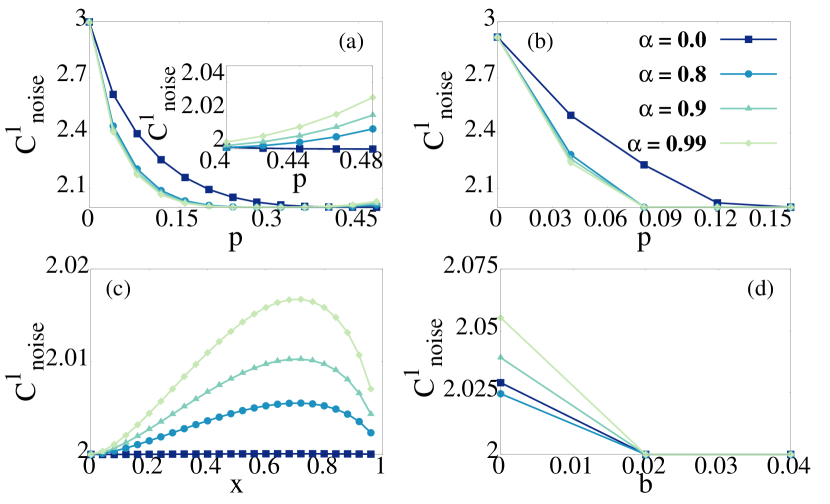
Figure 1: (Color online.) Two senders and a single receiver, $2\mathcal{S}-1\mathcal{R}$ case under non-Markovian dephasing noise. (a) and (b). $C^{1}_{\text{noise}}$ against the non-Markovian dephasing noise parameter, $p$ (abscissa) for different non-Markovianity, $\alpha$, when the shared resource states are the three-qubit GHZ and W states , which are affected by dephasing noise after encoding. The inset in (a) highlights the constructive effect of non-Markovianity at high noise strength. (c) and (d). DCC (ordinate) of three-qubit gGHZ and $|W_{1/2}\rangle^{3}$ states against the state parameters $x$ and $b$ (abscissa) respectively for $p=0.4$ . The different non-Markovianity parameters are represented from dark (blue) to light (green) as $\alpha=0.0$ (squares), $\alpha=0.8$ (circles), $\alpha=0.9$ (triangles) and $\alpha=0.99$ (diamonds) respectively. The $x$-axis is dimensionless whereas the $y$-axis is in bits.

III.1.1 Dense coding under non-Markovian noise

Let us now concentrate on the exact DCC affected by non-Markovian dephasing noise by performing numerical optimization. Let us now consider two exemplary sets of pure states as the shared resource, the gGHZ state and the generalized W state given by $|gW\rangle^{N+1}=\sum_{i}b_{i}\mathcal{P}[|0\rangle^{\otimes N}|1\rangle]$ where the $b_{i}$s are chosen to be real, and $\mathcal{P}$ denotes the permutation operator which permutes the vector $|1\rangle$ in different positions. The gW state for three-qubits Agrawal and Pati (2006); Roy et al. (2018), reduces to $|gW\rangle^{3}=\sqrt{a}|001\rangle+\sqrt{b}|010\rangle+\sqrt{1-a-b}|100\rangle$ where $a,b\in\mathbb{R}$ and $a+b\leq 1$ which, for $a=1/2$, exhibits perfect dense coding in the absence of noise and we refer to it as $|W_{1/2}\rangle^{3}$. For four-qubits, we can write it as $|gW\rangle^{4}=\sqrt{a}|0001\rangle+\sqrt{b}|0010\rangle+\sqrt{c}|0100\rangle+\sqrt{1-a-b-c}|1000\rangle$ (shared between $\mathcal{S}_{1},\mathcal{S}_{2},\mathcal{S}_{3}$ and $\mathcal{R}$) which has one ebit of entanglement for $a=1/2$ in the $\mathcal{S}:\mathcal{R}$ bipartition and we term it as $|W_{1/2}\rangle^{4}$. For these classes of states, we study the trends of DCC against the noise strength and the variation of state parameters, for different values of the non-Markovianity parameter, $\alpha$. In the case of the dephasing channel, the optimal unitary $U^{\min}$ is identified numerically (using the NLOPT algorithm ISRES Johnson ).

Two vs three senders with gGHZ states. When three- and four-qubit gGHZ states are shared between two and three senders respectively (with one receiver) and after encoding, the senders’ qubits are disturbed by dephasing noise, we obtain the noisy encoded state, denoted by $\rho^{gGHZ}_{(p,\alpha)}$ with $\rho^{gGHZ}_{(0,0)}$ being the original pure state. As one expects, $C^{1}_{\text{noise}}(\rho^{gGHZ}_{(p,0)})<C^{1}_{\text{noise}}(\rho^{gGHZ}_{(0,0)})$, i.e., the DCC decreases monotonically with the increase of the noise parameter $p$, irrespective of the state parameter. There exists a critical noise value $p_{c}$, where $C^{1}_{\text{noise}}(\rho^{gGHZ}_{(p,0)})$ reduces to its classical bound. For example, at $\alpha=0$, $p_{c}=0.48$ for the three-qubit gGHZ state while for four-qubit $|gGHZ\rangle^{4}$, $p_{c}=0.42$. Clearly, $p_{c}$ decreases with the number of senders, thereby showing a decrease in the robustness against noise with an increasing number of parties.

Constructive effects of non-Markovianity. Quantum advantage in the DC protocol emerges with high noise in the presence of strong non-Markovianity, i.e., a higher non-Markovian strength allows for countering the destructive effects of noise on the DCC. Specifically, at high $p$ and $\alpha$, we observe the existence of $p_{a}$, i.e., for $p\geq p_{a}$ $C^{1}_{\text{noise}}(\rho^{gGHZ}_{(p,\alpha)})>C^{1}_{\text{noise}}(\rho^{gGHZ}_{(p,0)})$, thereby establishing the constructive response of non-Markovianity (see Fig. 1 (a) and (c), and Table. 1). The advantage in DCC is more pronounced at high values of noise strength and non-Markovianity. In other words, $p_{a}$, as defined in Eq. (14), decreases with $\alpha$ and $p$. For the shared four-qubit gGHZ states, the quantum advantage can again be reported which are of two kinds - (i) $C^{1}_{\text{noise}}(|gGHZ\rangle^{4}_{(p,\alpha)})$ becomes non-vanishing after it collapses, i.e., $p_{r}$ exists like the three qubit case. (ii) Secondly, $C^{1}_{\text{noise}}(\rho^{gGHZ}_{(p,\alpha)})>C^{1}_{\text{noise}}(\rho^{gGHZ}_{(p,0)})$, thereby obtaining $p_{a}$. Notice that, for the existence of $p_{a}$, a high amount of non-Markovianity is required for three senders compared to DC with two senders. It possibly indicates that when there are more senders, noise acts on each channel, thereby accumulating more destructive effects of noise which can only be eliminated with high non-Markovianity as shown in Table. 1.

No advantage of non-Markovianity for generalized W states. In general, the DCC for the gW states, in the $N\mathcal{S}-1\mathcal{R}$ routine, neither revives after collapse nor shows advantage due to non-Markovian noise after collapse (see Table. 1). In particular, as shown in Fig. 1 (b), $p_{c}$ decreases with the strength of non-Markovianity $\alpha$, thereby illustrating less robustness of the $|W\rangle^{3}$ state against noise. However, the $|W_{1/2}\rangle^{3}$ states show an opposite behavior, especially constructive effect with $\alpha$. For example, for $p=0.4$ and sufficiently high non-Markovianity ($\alpha>0.8)$, we have $C^{1}_{\text{noise}}(|W_{1/2}\rangle^{3}_{(p,\alpha)})>C^{1}_{\text{noise}}(|W_{1/2}\rangle^{3}_{(p,0)})$. In spite of such advantage, states for which non-classical capacity does not exist under Markovian noise ($b\leq 0.02$ as illustrated in Fig. 1(d)), fail to exhibit quantum advantage at $\alpha>0$.

Detrimental behavior observed for the non-Markovian depolarising channel. Like entanglement, the depolarising channel has a much more adverse effect on the dense coding protocol than the dephasing one which is clear from the very low value of $p_{c}$ reported in Table. 2. This is primarily due to the fact that the depolarising noise acts on the qubits from all directions in contrast to the dephasing type noise which only affects the qubits from the z-direction Gupta et al. (2022). Neither the gGHZ nor the gW states show any advantage with $\alpha$, rather, their capacities decrease with non-Markovianity. As argued before, non-Markovianity can counter the destructive effects of noise only when the noise strength is above a certain threshold value which is not possible for the depolarizing channel since the noise parameter (p) is upper bounded by $1/3\alpha$ for any arbitrary shared state. Moreover, comparing the $2\mathcal{S}-1\mathcal{R}$ and the $3\mathcal{S}-1\mathcal{R}$ protocols, we find that the DCC is much worse affected for the three senders’ case than that of the two senders’ protocol.

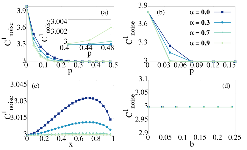
Figure 2: (Color online.) $3\mathcal{S}-1\mathcal{R}$ under non-Markovian dephasing noise. (a) and (b). $C^{1}_{\text{noise}}$ (ordinate) vs $p$ (abscissa) when four-qubit GHZ and W states are initially shared. The constructive effect of non-Markovianity at high $p$ and $\alpha$ is highlighted in the inset in (a). (c) and (d). DCC for the four-qubit gGHZ and $|W_{1/2}\rangle^{4}$ states with the state parameters, $x$ and $b$(abscissa) respectively for $p=0.4$. All other specifications are same as in Fig. 1.

III.2 Distributed non-Markovian dense coding

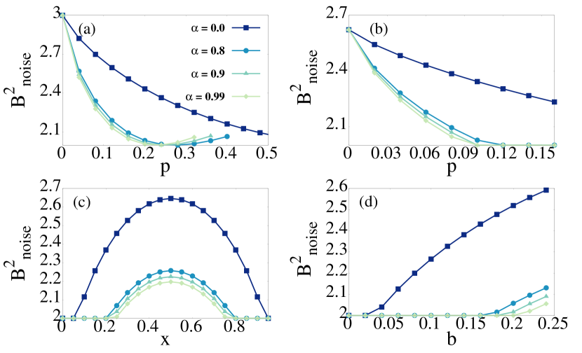
Figure 3: (Color online.) Two senders and two receivers scenario. $B^{2}_{\text{noise}}$ with non-Markovian depolarising noise, $p$ in (a) and (b) for the GHZ and W states while in (c) and (d), the upper bound on capacity is plotted against state parameters of gGHZ and $|W_{1/2}\rangle^{4}$. All other specifications are the same as in Fig. 1.

A dense coding scheme with two senders and two receivers is qualitatively different than the scenario with a single receiver. The impact of noise on the distributed dense coding protocol can only be inferred by studying the pattern of an upper bound $B^{2}_{noise}$ via LOCC in Eq. (LABEL:eq:DCC_2R_noisy).

We again consider the non-Markovian dephasing and depolarizing channels as noise models to obtain the expressions for the dense coding capacity given in Eq. (LABEL:eq:DCC_2R_noisy). In contrast to the single receiver scenario, we will show that the two-receiver dense coding protocol is more robust to the non-Markovian dephasing noise (since $p_{c}$ does not exist for the gGHZ states in the $2\mathcal{S}-2\mathcal{R}$ regime), and the $|W_{1/2}\rangle^{4}$ states also provide a larger quantum advantage in DCC than the one-receiver scenario for both types of noise. Moreover, for the gGHZ states, the dephasing channel has no effect on the dense coding capacity when varied against $\alpha$ i.e., $B^{2}_{\text{noise}}(|gGHZ\rangle^{4})$ is invariant for the entire range of non-Markovianity at a fixed noise strength $p$.

Theorem 3. For the four-qubit gGHZ state shared between two senders and two receivers, the upper bound on the distributed DCC without noise coincides with the upper bound in the presence of non-Markovian dephasing noise, i.e., $B^{2}_{\text{noise}}=B^{2}$ irrespective of the value of the non-Markovian parameter $\alpha$.

Proof. The four-qubit gGHZ state, $|gGHZ\rangle^{4}_{\mathcal{S}_{1}\mathcal{S}_{2}\mathcal{R}_{1}\mathcal{R}_{2}}=x|0000\rangle+\sqrt{1-x^{2}}|1111\rangle$ can be represented in the density matrix form as $\rho_{gGHZ}=x^{2}|0000\rangle\langle 0000|+(1-x^{2})|1111\rangle\langle 1111|+x\sqrt{(1-x^{2})}(|0000\rangle\langle 1111|+|1111\rangle\langle 0000|)$. If we again assume that the $U^{\min}$ are proportional to the identity operator, which our numerical studies show to be the case, the non-Markovian noise does not change the subspace of the affected state, i.e., $\Lambda(\rho_{gGHZ})=x^{2}|0000\rangle\langle 0000|+(1-x^{2})|1111\rangle\langle 1111|+f(p,\alpha,x)(|0000\rangle\langle 1111|+|1111\rangle\langle 0000|)$ where the function $f$ includes the noise parameters $p$ and $\alpha$. Notice that only the off-diagonal terms change, which does not contribute during the partial trace operation, unlike the single receiver protocol. The only term in the expression of $B^{2}_{\text{noise}}$ that can get modified by the effect of noise is $\max[S(\text{Tr}_{\mathcal{S}_{1}\mathcal{R}_{1}}\Lambda(\rho_{gGHZ})),S(\text{Tr}_{\mathcal{S}_{2}\mathcal{R}_{2}}\Lambda(\rho_{gGHZ}))]=H(\{x^{2},1-x^{2},0,0\})$ which is independent of the non-Markovianity parameter $\alpha$ and also the noise strength $p$. Thus independent of the value of $\alpha$ and $p$, the upper bound on the $2\mathcal{S}-2\mathcal{R}$ DCC remains unchanged and equal to its noiseless value $B^{2}_{\text{noise}}=2+H(\{x^{2},1-x^{2}\})$ bits. Hence the proof. $\hfill\blacksquare$
Remark. The optimizing unitaries $U^{\min}$ appearing in Eq. (LABEL:eq:DCC_2R_noisy) do not make any qualitative changes to our results since numerical studies suggest that each $U^{\min}$ acting on the sender’s end, is proportional to the identity operator, and thus do not change the subspace to which the initial state belongs.
Let us now elaborate on our numerical observations pertaining to the noisy distributed dense coding scheme.

• gGHZ states - dephasing vs depolarizing noise. Although no non-Markovian advantage is reported for the dephasing channel in the entire parameter range of $\alpha$ for the gGHZ state, the GHZ state remains unaffected by non-Markovianity, furnishing $B^{2}_{\text{noise}}=2+H(\{x^{2},1-x^{2}\})$ for all $\alpha$. There is, however, a destructive effect on the DCC of the gGHZ states against depolarising noise, such that $B^{2}_{\text{noise}}$ decreases with $\alpha>0$ although it remains above the classical threshold as illustrated in Figs. 3(a) and (c).

• gW states. For the dephasing type of noise, the dense coding capacity of the W state does not hit the classical value at all but decreases to a minimum value and the quantum advantage also increases with $\alpha$ as shown in Table. 1. On the contrary, the depolarising noise is again destructive in nature whence the capacity decreases with an increase of the non-Markovian parameter. The W state, according to Fig. 3 (b) shows no advantage of non-Markovianity for the depolarising channel and the capacity collapses to its classical limit faster than in the Markovian regime. The $|W_{1/2}\rangle^{4}$ state also mimics this behavior, where the DCC decreases with $\alpha$ and the parameter regime of $b$ where quantum advantage exists also shrinks with non-Markovianity as shown in Fig. 3(d).

Table 2: Critical noise strength $p_{c}$ for GHZ and W states affected by non-Markovian depolarising noise.

$\alpha$	$p_{c}$
	GHZ			W
	$2\mathcal{S}-1\mathcal{R}$	$3\mathcal{S}-1\mathcal{R}$	$2\mathcal{S}-2\mathcal{R}$	$2\mathcal{S}-1\mathcal{R}$	$3\mathcal{S}-1\mathcal{R}$	$2\mathcal{S}-2\mathcal{R}$
0	0.09	0.06	0.75	0.08	0.05	0.31
0.3	0.07	0.03	0.58	0.05	0.03	0.26
0.5	0.05	0.03	0.45	0.04	0.02	0.21
0.7	0.04	0.02	0.32	0.03	0.02	0.16
0.9	0.03	0.02	0.25	0.02	0.02	0.1

IV Effects of random channels on Dense Coding Capacity

In this section, we study the impact of noise on dense coding protocol, when the noisy channels are characterized by random unitaries along with non-Markovianity as discussed in Sec. II.2. Note that in case of random noise, the DCC has to be computed by performing averaging which we define now.

Quenched averaging. For a fixed resource state and non-Markovianity $\alpha$, in a single realization, we compute $C^{1}_{noise}$ or $B^{2}_{noise}$ by choosing a set of parameters in the unitary, $\{x_{i}\}$, from a Gaussian distribution with mean $\langle x_{i}\rangle$ and standard deviation $\epsilon$. We calculate the dense coding capacity for $4\times 10^{3}$ sets of such realizations and by averaging them, we obtain quenched averaged dense coding capacity denoted by $\langle C^{1}_{noise}\rangle$ or $\langle B^{2}_{noise}\rangle$.

Theorem 4. The upper bound on the dense coding capacity affected by the random noisy channel for multiple senders and a single receiver is greater than the capacity influenced by noise without randomness.

Proof. Any arbitrary unitary operator in two dimensions can be characterized by three parameters $\omega,\theta$, and $\delta$, apart from an overall phase, as in Eq. (9). Let us suppose that the noise consisting of any Pauli matrix is written as $U^{o}=U_{1}^{o}U_{2}^{o}U_{3}^{o}$, characterized by the parameters $\omega^{o},\theta^{o}$, and $\delta^{o}$ respectively. Suppose, the random unitary corresponding to $U^{o}$ is $U=U_{1}U_{2}U_{3}$. To generate such a random unitary, each parameter, ($\omega,\theta$, and $\delta$) is randomly chosen from a Gaussian distribution of mean $\omega^{o},\theta^{o}$, and $\delta^{o}$ respectively and standard deviation $\epsilon$. Thus one arbitrary choice of the parameters of the random unitary $U$ may be taken to be $\omega^{o}+\epsilon,\theta^{o}+\epsilon,\delta^{o}+\epsilon$. It can be shown that the unitaries constituting $U$ can be written as $U_{i}=\cos\frac{\epsilon}{2}U_{i}^{o}+\sin\frac{\epsilon}{2}U_{i}^{\prime}$ with $i=1,2,3$ where

$$U_{1}^{\prime}=\begin{pmatrix}ie^{i\omega/2}&0\\ 0&-ie^{-i\omega/2}\end{pmatrix},$$

$$U_{2}^{\prime}=\begin{pmatrix}-\sin\theta/2&\cos\theta/2\\ -\cos\theta/2&-\sin\theta/2\end{pmatrix},$$

$$U_{3}^{\prime}=\begin{pmatrix}ie^{i\delta/2}&0\\ 0&-ie^{-i\delta/2}\end{pmatrix}.$$ (16)

Thus $U=U_{1}U_{2}U_{3}=\cos^{3}\frac{\epsilon}{2}U^{0}+\sum_{i}f_{i}(\epsilon)\tilde{U}_{i}$, where each $f_{i}(\epsilon)=\mathcal{O}(\sin\frac{\epsilon}{2})$ or higher and each $\tilde{U}_{i}$ represents a unitary obtained from the product of $U_{i}^{\prime}s$ and $U^{o}$. Finally, we can write the action of $U$ on a state $\rho$ as

$$U\rho U^{\dagger} =\cos^{6}\frac{\epsilon}{2}U^{o}\rho U^{o\dagger}+\sum_{i}f_{i}(\epsilon)U^{o}\rho\tilde{U}_{i}^{\dagger}+\sum_{i}f_{i}(\epsilon)\tilde{U}_{i}\rho U^{o\dagger}$$ (18)

$$+\sum_{i,j}f_{i}(\epsilon)f_{j}(\epsilon)\tilde{U}_{i}\rho\tilde{U}_{j}^{\dagger}$$

$$=\cos^{6}\frac{\epsilon}{2}U^{o}\rho U^{o\dagger}+\sum_{\begin{subarray}{c}i,j\\ j\neq i\end{subarray}}f_{i}(\epsilon)f_{j}(\epsilon)\tilde{U}_{i}\rho\tilde{U}_{j}^{\dagger}.$$

Here, the condition $i\neq j$ takes care to omit the repetition of the term $U^{o}\rho U^{o\dagger}$ in the summation.

Let us now illustrate the proof for the dephasing channel. Note that the same line of proof would hold for the depolarising channel, but with some more cumbersome algebra. The dephasing channel is characterized by the Pauli operator $U^{o}=\sigma_{z}$ whose parameters $\omega^{o},\theta^{o}$ and $\delta^{o}$ are given in Sec. II.2. Since we consider the noise to act only on the senders’ part, the only affected term in the dense coding capacity given by Eq. (2) is $S(\tilde{\rho})$. In the presence of a random dephasing channel, we can write $S(\tilde{\rho}_{random})=S(p_{1}\rho+p_{2}U\rho U^{\dagger})$, where $p_{1}=(1-\alpha p)(1-p)$ and $p_{2}=(1+\alpha(1-p))p$ with $p$ being the noise parameter of the dephasing channel and $\alpha$, the strength of non-Markovianity. Using concavity of entropy, Nielsen and Chuang (2000), i.e., $S(\sum_{i}p_{i}\rho_{i})\leq\sum_{i}p_{i}S(\rho_{i})+H\{p_{i}\}$, we obtain

$$S(p_{1}\rho+\cos^{6}\frac{\epsilon}{2}p_{2}U^{o}\rho U^{o\dagger}+p_{2}\sum_{\begin{subarray}{c}i,j\\ j\neq i\end{subarray}}f_{i}(\epsilon)f_{j}(\epsilon)U_{i}\rho U_{j}^{\dagger})$$ (19)

$$\leq S(p_{1}\rho+\cos^{6}\frac{\epsilon}{2}p_{2}U^{o}\rho U^{o\dagger})+p_{2}\sum_{\begin{subarray}{c}i,j\\ j\neq i\end{subarray}}f_{i}(\epsilon)f_{j}(\epsilon)S(U_{i}\rho U_{j}^{\dagger})$$

$$~{}~{}~{}~{}~{}~{}~{}~{}~{}~{}~{}~{}~{}~{}~{}~{}~{}~{}~{}~{}~{}~{}~{}~{}+H\{p_{1},p_{2},p_{2}f_{i}(\epsilon)f_{j}(\epsilon)\}.$$ (20)

We can neglect the last summation, since each $f_{i}(\epsilon)$ is a function of $\sin\epsilon$ and we have assumed $\epsilon\to 0$, which also implies $\cos^{6}\epsilon\to 1$. Thus we finally arrive at

$$S(\tilde{\rho}_{random})\leq S(\tilde{\rho}_{dph})+H\{p_{1},p_{2}\}$$ (21)

$$\implies C^{1}_{\text{noise}}(\Lambda_{\text{random}}(\rho))\geq C^{1}_{\text{noise}}(\Lambda_{\text{dph}}(\rho))-$$

$$~{}~{}~{}~{}~{}~{}~{}~{}~{}~{}~{}~{}~{}~{}~{}~{}~{}~{}~{}~{}~{}~{}~{}~{}~{}~{}~{}~{}~{}~{}~{}~{}~{}~{}~{}~{}~{}~{}~{}~{}~{}~{}~{}~{}~{}~{}~{}~{}~{}H\{p_{1},p_{2}\}.$$ (22)

Numerical simulations confirm that $S(\tilde{\rho}_{random})\leq S(\tilde{\rho}_{dph})$ for small as well as moderate disorder strength, $\epsilon$. Therefore, the dense coding capacity for a state affected by random noise is greater than that affected by Pauli noise. $\hfill\blacksquare$

Remark. In case of dephasing channel, $U^{\min}$ is again chosen to be the identity operator in the proof for simplicity. However, numerical simulations again show that the results remain true even when optimization over unitaries are performed.

Table 3: Critical noise strength for collapse, $p_{c}$, for GHZ and W states affected by random depolarising noise.

	GHZ						W
	$2\mathcal{S}-1\mathcal{R}$			$3\mathcal{S}-1\mathcal{R}$			$2\mathcal{S}-1\mathcal{R}$			$3\mathcal{S}-1\mathcal{R}$
$\alpha$	$\epsilon=0.5$	$\epsilon=0.7$	$\epsilon=1.0$	$\epsilon=0.5$	$\epsilon=0.7$	$\epsilon=1.0$	$\epsilon=0.5$	$\epsilon=0.7$	$\epsilon=1.0$	$\epsilon=0.5$	$\epsilon=0.7$	$\epsilon=1.0$
0.3	0.09	0.11	0.14	0.04	0.05	0.06	0.08	0.09	0.12	0.03	0.04	0.05
0.5	0.06	0.08	0.1	0.03	0.04	0.05	0.05	0.06	0.09	0.03	0.03	0.04
0.9	0.04	0.05	0.07	0.02	0.03	0.04	0.03	0.04	0.07	0.02	0.02	0.01

IV.1 Random noise of the dephasing type

To begin our discussion on the effect of random noisy channels, we first consider the dephasing channel composed of two Kraus operators, one involving the identity, and the other involving $\sigma_{z}$. In the case of random channels, the parameters of unitaries are chosen from a Gaussian distribution of standard deviation $\epsilon$ and mean fixed to the parameters of the corresponding Pauli matrix. We notice that the presence of such random noise provides a distinct advantage in the dense coding protocol in comparison with the effects of a pure dephasing channel, i.e., $C^{1}_{\text{noise}}(\Lambda_{p,\alpha,\epsilon}(\rho))\geq C^{1}_{\text{noise}}(\Lambda_{p,\alpha,0}(\rho))$, where $\epsilon$ denotes the magnitude of randomness present in the noise. Let us present our observations for the case of single- and two receivers scenarios.

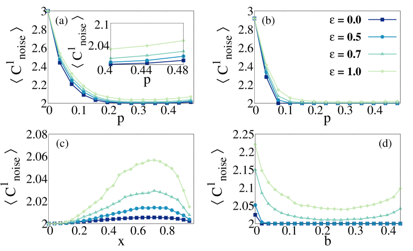
Figure 4: (Color online.) $2\mathcal{S}-1\mathcal{R}$ DC with random non-Markovian dephasing noise. Quenched averaged dense coding capacity, $\langle C^{1}_{\text{noise}}\rangle$, (ordinate) with different disorder strength, $\epsilon$ against the noise parameter $p$ in (a). and (b)., and against the state parameter $x$ and $b$ (abscissa) in (c). and (d) respectively. The states shared between senders and the receiver are the three-qubit GHZ (in (a)), W (in (b)), gGHZ (in (c)), and $|W_{1/2}\rangle^{3}$ states (in (d)). Squares, circles, triangles and diamonds represent $\epsilon=0$, $\epsilon=0.5$, $\epsilon=0.7$ and $\epsilon=1.0$ respectively. In all the cases, the non-Markovianity parameter is fixed to $\alpha=0.8$. The horizontal axis is dimensionless although the vertical axis is in bits.

IV.1.1 Random channel-effected dense coding involving a single receiver: Comparison between gGHZ and gW states

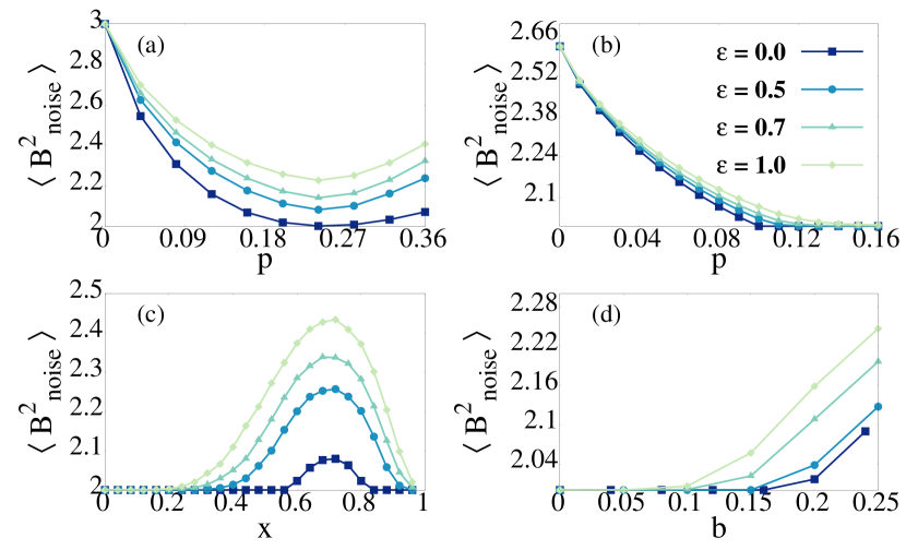
Figure 5: (Color online.) The average upper bound on DCC under random non-Markovian depolarising noise when $\alpha=0.9$. All other specifications are the same as in Fig. 4.

$2\mathcal{S}$-$1\mathcal{R}$ case. In the case of the three-qubit GHZ state, we find that the average capacity increases steadily with $\epsilon$ for any value of $\alpha$ as shown in Fig. 4 (a). In fact, for sufficiently high standard deviation, e.g. $\epsilon\geq 0.7$, the quenched dense coding capacity does not collapse to its classical threshold (which is $2$) but reaches a minimum value ($\geq 2$) and then rises again with the noise strength $p$. In this case, $p_{a}$ decreases with respect to both $\alpha$ and $\epsilon$. The decrease in $p_{a}$ with $\epsilon$ predicts the beneficial impact of randomness present in the noise acting on the protocol. Qualitatively similar behavior is observed when the W state is considered as the resource (see Fig. 4 (b).). This demonstrates that if the dephasing channel is not perfect, the protocol is much more beneficial in terms of dense coding capacity.

When analyzed with respect to the state parameter, we observe that the protocol becomes more and more efficient for a given $\alpha$ as the standard deviation $\epsilon$ assumes higher and higher values for the $|gGHZ\rangle^{3}$ and $|W_{1/2}\rangle^{3}$ states. For any given non-Markovianity strength and standard deviation, the capacity becomes maximum at $x=1/\sqrt{2}$ for the GHZ state as demonstrated in Fig. 4 (c). An important feature of randomly generated dephasing type noise emerges - there exist some p and x for which the Markovian pure dephasing channel offers no quantum advantage with the $|W_{1/2}\rangle^{3}$ state although an increase in the standard deviation makes the capacity overcome the classical limit. Thus the constructive effect of randomness is again highlighted in the noisy DC protocol.

$3\mathcal{S}$-$1\mathcal{R}$ scenario. The advantageous effect of randomness still persists when we consider $|GHZ\rangle^{4}$ but is much less pronounced, with the revival of capacity beyond its classical value (upon collapse) being absent. Thus, with an increase in the number of senders, the destructive effect of the noise cannot be avoided through its random implementation, since more qubits are affected by it. In the protocol involving three senders sharing a W state with a lone receiver, no quantum advantage beyond that for the pure dephasing channel is apparent no matter how high the value of $\epsilon$ is. For the $|gGHZ\rangle^{4}$ states, the random noise cannot help in overcoming the classical limit of $3$ for any value of $\epsilon$ or $\alpha$. On the other hand, for sufficiently high randomness ($\epsilon\geq 0.5$), some quantum advantage is observed for $|W_{1/2}\rangle^{4}$.

IV.1.2 Effects of random noise on distributed dense coding

When the dense coding protocol involves two receivers, we consider four qubit resource states shared between two senders and two receivers. The principal difference in the dense coding protocol involving two receivers, from that having a single receiver, is that the random noisy channel exhibits no effect when considering the gGHZ states. The constructive effect of randomness is observed for the W and $|W_{1/2}\rangle^{4}$ states, in Figs. 7 (b) and (d) respectively, where the quenched averaged capacity increases with $\epsilon$ (however, it still remains lower than the gGHZ states). Unlike the gGHZ state, for which the region of quantum advantage is stretched across the entire parameter regime, the $|W_{1/2}\rangle^{4}$ states demonstrate quantum advantage only beyond $b\approx 0.1$.

IV.2 Depolarising random noise on dense coding: Beneficial role

We have already observed that depolarizing channels acting on the encoded qubits has extremely damaging effects on the performance of DC. It will be interesting to find out whether random channels can have a more destructive impact or less. Our results can be listed according to the resource states.

1. gGHZ state as resource. Although the pure Markovian depolarising channel suppresses any quantum advantage, an increase in $\epsilon$ at $\alpha=0$ causes an increment in the quenched averaged capacity beyond its classical value both in the $2\mathcal{S}-1\mathcal{R}$ and $3\mathcal{S}-1\mathcal{R}$ regimes. The advantage in the dense coding capacity is pronounced around $x=1/\sqrt{2}$ with the region of advantage increasing with an increase in the standard deviation (see Table. 3 for the GHZ state ($x=\frac{1}{\sqrt{2}}$)). However, the $\langle C^{1}_{noise}\rangle$ decreases with $\alpha$ for a given randomness parameter $\epsilon$ as demonstrated in Fig. 6 and Fig. 5 (c). Moreover, we observe that the critical noise strength of collapse, $p_{c}$, increases with the randomness, thereby sustaining non-classical capacity for a large range of the noise parameter.

   

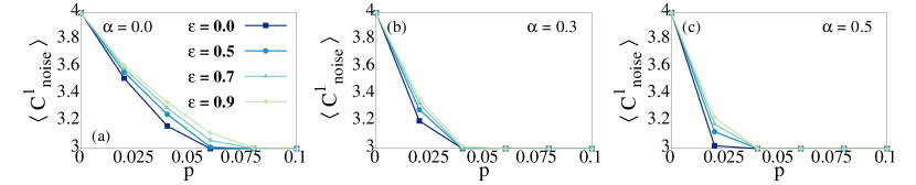
   Figure 6: (Color online.) Advantage in random depolarizing noise in $3\mathcal{S}-1\mathcal{R}$ DC protocol. $\langle C^{1}_{\text{noise}}\rangle$ (ordinate) against $p$ (abscissa) for different disorder strengths with the shared four-qubit GHZ state. Markovian noise, i.e., $\alpha=0.0$, (in (a)) is compared with non-Markovian noise, $\alpha=0.3$ (in (b)) and $\alpha=0.5$ (in (c)) respectively. All other specifications are the same as in Fig. 4.

   The situation is similar when the four-qubit gGHZ state is shared in the $2\mathcal{S}-2\mathcal{R}$ case. The averaged capacity here undergoes improvements with increasing $\epsilon$, as shown in Fig. 5 (a). The most important constructive feature is that for sufficient randomness in the channel ($\epsilon>0.5$), the quenched average capacity never reduces to its classical value of $2$, but rises after reaching a minimum value. This is in contrast to the depolarising noise without randomness, where revival is observed after the capacity becomes $2$. When the capacity attains a minimum value, an increase in the standard deviation increases the noise strength at which the minimum occurs, thereby again exhibiting a constructive effect since the capacity remains high through a large noise parameter regime.

   

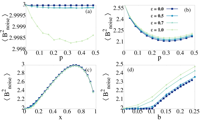
   Figure 7: (Color online.) The quenched averaged upper bound on the dense coding capacity, $\langle B^{2}_{\text{noise}}\rangle$, (ordinate) is demonstrated under random non-Markovian dephasing noise with $\alpha=0.9$ in two senders-two receivers picture. All other specifications are the same as in Fig. 4.

2. gW state. When a single receiver is involved in the dense coding protocol, the behavior of the averaged capacity of the gW state is similar to that of the gGHZ state, even though the quantum advantage is markedly less. The random noise allows for constructive effect in the two receivers scenario (see Fig. 5 (b).) whereas the pure depolarising channel always caused the capacity to decrease with $\alpha$, i.e., the random channel causes an increase in the DCC with increasing $\epsilon$. Moreover, the probability of collapse $p_{c}$, also increases with the standard deviation (see Table. 3). However, the noise strength of collapse is lower for the W state as compared to that for the GHZ state, thereby highlighting the increased susceptibility of the W state to noise.

3. A special class of gW state. For $|W_{1/2}\rangle^{3}$ and $|W_{1/2}\rangle^{4}$ shared with a single receiver, the dense coding capacity can never overcome its classical threshold in presence of non-Markovian noise. However, as illustrated in Fig. 5 (d), a constructive impact of randomness is apparent in the $2\mathcal{S}-2\mathcal{R}$ regime where the quenched average upper bound $\langle B^{2}_{noise}\rangle$ increases beyond the classical bound with an increase in $\epsilon$. Further, the state parameter region beyond which quantum advantage is obtained also expands with $\epsilon$ (for example at $\epsilon=0.3,\langle B^{2}_{noise}\rangle>2$ for $b\geq 0.15$ whereas $\langle B^{2}_{noise}\rangle>2$ beyond $b=0.1$ when $\epsilon=0.7$), thereby providing a two-fold advantage in the protocol.

V Conclusion

Quantum superdense coding illustrates quantum advantage for transferring classical information encoded in quantum states provided an entangled state is apriori shared between the senders and the receivers. To date, all the studies performed on the dense coding protocol have been solely focused on how Markovian noise affects the system’s encoded component. In a multipartite domain with arbitrary senders and one or two receivers, we found that when non-Markovian dephasing noise acts on the encoded part (especially for the three-party generalized Greenberger-Horne-Zeilinger(gGHZ) shared state), the dense coding capacity increases with an increase in non-Markovianity. This non-Markovian enhancement is less prominent eiter when the shared state is the W-state or when one increases the number of parties.

From the experimental point of view, the actions of exact dephasing or depolarising noise involving Pauli matrices on the sender’s part is extremely idealized situation. In reality, there must be some deviation from the Pauli noisy channel. In this work, we addressed the question of how the dense coding capacity gets affected if we choose Kraus representations involving unitaries from a Gaussian distribution with a mean around Pauli noise and a finite standard deviation. We dealt with multiple senders and single or two receivers sharing multipartite entangled states as the resource. Most strikingly, we showed both analytically and numerically that in presence of random noisy channels, the dense coding capacity increases with the increase of the strength of the randomness in the channel. Our work also indicates that non-Markovianity and random unitaries used in enhancing the performance of the dense coding protocol have a trade-off relation.

Appendix A Non-Markovian noisy channels

Noise acts on the states after encoding at the sender’s end occurs. In this work, we concentrate on two channels, the dephasing, and the depolarising channels. The non-Markovian versions of the aforementioned channels are parameterized by the non-Markovianity parameter $\alpha$ and the noise strength $p$. The Kraus operators for the dephasing and depolarising channels take the form as Shrikant et al. (2018)

$$K_{I}^{dph}=\sqrt{[1-\alpha p](1-p)}\mathbb{I},K_{z}^{dph}=\sqrt{[1+\alpha(1-p)]p}\sigma_{z},$$

$$K_{I}^{dp}=\sqrt{[1-3\alpha p](1-p)}\mathbb{I},K_{i}^{dp}=\sqrt{\frac{[1+3\alpha(1-p)]p}{3}}\sigma_{i}.$$

Here, $\sigma_{i}$ with $i=x,y,z$ represent the well-known Pauli matrices and the non-Markovianity parameter $\alpha$ lies between $0$ and $1$. For the dephasing channel, we have $0\leq p\leq 0.5$ whereas for the depolarising channel $p$ runs from $0$ to $1/3\alpha$. The Markovian limit is recovered by choosing $\alpha=0$, and a higher value of $\alpha$ corresponds to a higher amount of non-Markovianity in the channel Daffer et al. (2004).

Appendix B Noisy dense coding involving a Bell state

Let us consider that the Bell state $|\phi^{+}\rangle_{\mathcal{S}\mathcal{R}}=(1/\sqrt{2})(|00\rangle+|11\rangle)$ is shared between a sender, $\mathcal{S}$ and a receiver, $\mathcal{R}$. Upon encoding, the channel through which $\mathcal{S}$ sends the qubit to $\mathcal{R}$ is either a non-Markovian dephasing channel or a depolarising one. The dense coding capacity is given by

$$C^{1}_{\text{noise}}(|\phi^{+}\rangle_{\mathcal{S}\mathcal{R}})=2-S(\Lambda(U^{\min}|\phi^{+}\rangle_{\mathcal{S}\mathcal{R}}\langle\phi^{+}|U^{{\min}^{\dagger})}).$$ (25)

For analytical simplicity, we will not consider the unitaries $U^{\min}$ while calculating the capacity. This will not make any qualitative changes in the end result. Note that, the state is said to be dense codeable when $S(\Lambda(|\phi^{+}\rangle_{\mathcal{S}\mathcal{R}}\langle\phi^{+}|))\leq 1$.
Let us first consider the depolarising channel. The eigenvalues of $\Lambda(|\phi^{+}\rangle_{\mathcal{S}\mathcal{R}}\langle\phi^{+}|)$ are given by $\{x,(1-x)/3,(1-x)/3,(1-x)/3\}$ where $x=(1-p)(1-3\alpha p)$ when $\alpha>0$ which reduces to $x=(1-p)$ in the Markovian limit. It can easily be shown that the entropy term is below $1$ when $p\leq 1/3\alpha$, which is the range of operation for the depolarising channel. By setting $\alpha=0$, we find that in the case of the Markovian channel, the state remains dense codeable as long as $p\lesssim 0.19$. Now, given the set of eigenvalues of the noisy state, it is evident that the maximum of $S(\Lambda(|\phi^{+}\rangle_{\mathcal{S}\mathcal{R}}\langle\phi^{+}|))$ occurs when $x=0.25$. For the Markovian case, we have $(1-p)\geq 0.25$ and $p/3\leq 0.25$. Conversely, when $\alpha>0$, $(1-p)(1-3\alpha p)\geq 0.25$ and $p(1+3\alpha(1-p))/3\leq 0.25$. Note that if the eigenvalue less than $0.25$ is greater in the non-Markovian case as compared to the Markovian limit, then the last entropy term is also greater when $\alpha\neq 0$. We can indeed observe that $S(\Lambda_{NM}(|\phi^{+}\rangle_{\mathcal{S}\mathcal{R}}\langle\phi^{+}|))\geq S(\Lambda_{M}(|\phi^{+}\rangle_{\mathcal{S}\mathcal{R}}\langle\phi^{+}|))$ and the dense coding capacity for the non-Markovian case is lower than that of the Markovian case when the noisy channel is depolarising in nature.

We now move on to the case of the dephasing channel. The eigenvalues of the noisy resource in this case read as $\{\frac{1}{2}(1\pm\sqrt{1+4p(p-1)(\alpha(p-1)-1)(\alpha p-1)})\}$. Comparing the last term in the DCC for Markovian and non-Markovian channels, Since the eigenvalues are symmetric around $1/2$, we can conclude that $S(\Lambda_{NM}(|\phi^{+}\rangle_{\mathcal{S}\mathcal{R}}\langle\phi^{+}|))\leq S(\Lambda_{M}(|\phi^{+}\rangle_{\mathcal{S}\mathcal{R}}\langle\phi^{+}|))$ when the lower eigenvalue for $\alpha>0$ is less than the lower eigenvalue for $\alpha=0$ (which implies that the higher eigenvalue in the non-Markovian case is greater than that in the Markovian limit). Let us define $l$ as the difference between the lower eigenvalues of the Markovian and non-Markovian cases. It can easily be verified that as $\alpha\to 1$ and $p\to 0.5$, $l\geq 0$ since its minimum value is zero and its maximum value $\approx 0.18$. Thus in the limit of high noise strength and high non-Markovian parameter, the entropy term for the non-Markovian channel is lower than that of the corresponding Markovian one. Therefore, the dense coding capacity of the non-Markovian channel is greater than that for $\alpha=0$. On the other hand, as $p\to 0$, the dense coding capacity at low noise strengths is higher for the Markovian channel than that of the non-Markovian one. Thus in the case of dephasing noise, non-Markovianity allows for an advantage over the Markovian regime only when the noise strength and the non-Markovian parameter both take high values.

References

- Horodecki et al. (2009) R. Horodecki, P. Horodecki, M. Horodecki, and K. Horodecki, Rev. Mod. Phys. 81, 865 (2009).
- Bennett and Wiesner (1992) C. H. Bennett and S. J. Wiesner, Phys. Rev. Lett. 69, 2881 (1992).
- Bennett et al. (1993) C. H. Bennett, G. Brassard, C. Crépeau, R. Jozsa, A. Peres, and W. K. Wootters, Phys. Rev. Lett. 70, 1895 (1993).
- Ekert (1991) A. K. Ekert, Phys. Rev. Lett. 67, 661 (1991).
- Raussendorf and Briegel (2001) R. Raussendorf and H. J. Briegel, Phys. Rev. Lett. 86, 5188 (2001).
- Bose et al. (2000) S. Bose, M. Plenio, and V. Vedral, J. Mod. Opt. 47, 291 (2000).
- Bowen (2001) G. Bowen, Phys. Rev. A 63, 022302 (2001).
- Liu et al. (2002) X. S. Liu, G. L. Long, D. M. Tong, and F. Li, Phys. Rev. A 65, 022304 (2002).
- Ziman and Bužek (2003a) M. Ziman and V. Bužek, Phys. Rev. A 67, 042321 (2003a).
- Hiroshima (2001) T. Hiroshima, J. Phys. A: Mathematical and General 34, 6907 (2001).
- Bruß et al. (2014) D. Bruß, G. M. D’Ariano, M. Lewenstein, C. Macchiavello, A. Sen(De), and U. Sen, Phys. Rev. Lett. 93, 210501 (2014).
- Bruß et al. (2006) D. Bruß, M. Lewenstein, A. Sen(De), U. Sen, D. G. M., and C. Macchiavello, International Journal of Quantum Information 4, 415 (2006).
- Laurenza et al. (2020) R. Laurenza, C. Lupo, S. Lloyd, and S. Pirandola, Phys. Rev. Research 2, 023023 (2020).
- Mattle et al. (1996) K. Mattle, H. Weinfurter, P. G. Kwiat, and A. Zeilinger, Phys. Rev. Lett. 76, 4656 (1996).
- Shimizu et al. (1999) K. Shimizu, N. Imoto, and T. Mukai, Phys. Rev. A 59, 1092 (1999).
- Mizuno et al. (2005) J. Mizuno, K. Wakui, A. Furusawa, and M. Sasaki, Phys. Rev. A 71, 012304 (2005).
- Pan et al. (2012) J.-W. Pan, Z.-B. Chen, C.-Y. Lu, H. Weinfurter, A. Zeilinger, and M. Żukowski, Rev. Mod. Phys. 84, 777 (2012).
- Northup and Blatt (2014) T. E. Northup and R. Blatt, Nature Photonics 8, 356 (2014).
- Barreiro et al. (2014) J. T. Barreiro, T.-C. Wei, and P. G. Kwiat, Nature Physics 4, 282 (2014).
- Krenn et al. (2016) M. Krenn, J. Handsteiner, M. Fink, R. Fickler, R. Ursin, M. Malik, and A. Zeilinger, Proceedings of the National Academy of Sciences 113, 13648 (2016).
- Fang et al. (2000) X. Fang, X. Zhu, M. Feng, X. Mao, and F. Du, Phys. Rev. A 61, 022307 (2000).
- Leibfried et al. (2003) D. Leibfried, R. Blatt, C. Monroe, and D. Wineland, Rev. Mod. Phys. 75, 281 (2003).
- Vandersypen and Chuang (2005) L. M. K. Vandersypen and I. L. Chuang, Rev. Mod. Phys. 76, 1037 (2005).
- Yang and Gong (2007) W. Yang and Z. Gong, Journal of Physics B: Atomic, Molecular and Optical Physics 40, 1245 (2007).
- Gross et al. (2009) D. Gross, S. T. Flammia, and J. Eisert, Phys. Rev. Lett. 102, 190501 (2009).
- Hausladen et al. (1996) P. Hausladen, R. Jozsa, B. Schumacher, M. Westmoreland, and W. K. Wootters, Phys. Rev. A 54, 1869 (1996).
- Horodecki et al. (2001) M. Horodecki, P. Horodecki, R. Horodecki, D. Leung, and B. Terhal, (2001), 10.48550/ARXIV.QUANT-PH/0106080.
- Holevo (1973) A. S. Holevo, Probl. Peredachi Inf. 9, 3 (1973).
- Holevo (1998) A. Holevo, IEEE Transactions on Information Theory 44, 269 (1998).
- Sen (De) A. Sen(De) and U. Sen, Physics News 40, 17 (2010).
- Badzia¸g et al. (2003) P. Badzia¸g, M. Horodecki, A. Sen(De), and U. Sen, Phys. Rev. Lett. 91, 117901 (2003).
- Horodecki et al. (2004) M. Horodecki, J. Oppenheim, A. Sen(De), and U. Sen, Phys. Rev. Lett. 93, 170503 (2004).
- Ghosh et al. (2005) S. Ghosh, P. Joag, G. Kar, S. Kunkri, and A. Roy, Phys. Rev. A 71, 012321 (2005).
- Beran and Cohen (2008) M. R. Beran and S. M. Cohen, Phys. Rev. A 78, 062337 (2008).
- Shadman et al. (2011) Z. Shadman, H. Kampermann, D. Bruß, and C. Macchiavello, Phys. Rev. A 84, 042309 (2011).
- Shadman et al. (2012) Z. Shadman, H. Kampermann, D. Bruß, and C. Macchiavello, Phys. Rev. A 85, 052306 (2012).
- Gupta et al. (2021) R. Gupta, S. Gupta, S. Mal, and A. Sen(De), Phys. Rev. A 103, 032608 (2021).
- Wu et al. (2006) S. Wu, S. M. Cohen, Y. Sun, and R. B. Griffiths, Phys. Rev. A 73, 042311 (2006).
- Ji et al. (2006) Z. Ji, Y. Feng, R. Duan, and M. Ying, Phys. Rev. A 73, 034307 (2006).
- Bourdon et al. (2008) P. S. Bourdon, E. Gerjuoy, J. P. McDonald, and H. T. Williams, Phys. Rev. A 77, 022305 (2008).
- Tsai and Hwang (2010) C.-W. Tsai and T. Hwang, Optics Communications 283, 4397 (2010).
- Srivastava et al. (2019) C. Srivastava, A. Bera, A. Sen (De), and U. Sen, Phys. Rev. A 100, 052304 (2019).
- Hao et al. (2000) J.-C. Hao, C.-F. Li, and G.-C. Guo, Physics Letters A 278, 113 (2000).
- Feng et al. (2006) Y. Feng, R. Duan, and Z. Ji, Phys. Rev. A 74, 012310 (2006).
- Kögler and Neves (2017) R. A. Kögler and L. Neves, Quantum Information Processing 16, 92 (2017).
- Nielsen and Chuang (2000) M. Nielsen and I. Chuang, Quantum Computation and Quantum Information (Cambridge University Press, 2000).
- Breuer and Petruccione (2007) H.-P. Breuer and F. Petruccione, The Theory of Open Quantum Systems (Oxford University Press, 2007).
- Daffer et al. (2004) S. Daffer, K. Wódkiewicz, J. D. Cresser, and J. K. McIver, Phys. Rev. A 70, 010304 (2004).
- Rivas and Huelga (2012) A. Rivas and S. F. Huelga, Open Quantum Systems: An Introduction (SpringerBriefs in Physics, Springer, Spain, 2012).
- Shrikant et al. (2018) U. Shrikant, R. Srikanth, and S. Banerjee, Phys. Rev. A 98, 032328 (2018).
- Lidar (2019) D. A. Lidar, (2019), 10.48550/ARXIV.1902.00967.
- Yu and Eberly (2004) T. Yu and J. H. Eberly, Phys. Rev. Lett. 93, 140404 (2004).
- Dodd and Halliwell (2004) P. J. Dodd and J. J. Halliwell, Phys. Rev. A 69, 052105 (2004).
- Ficek and Tanaś (2006) Z. Ficek and R. Tanaś, Phys. Rev. A 74, 024304 (2006).
- Almeida et al. (2007) M. P. Almeida, F. de Melo, M. Hor-Meyll, A. Salles, S. P. Walborn, P. H. S. Ribeiro, and L. Davidovich, Science 316, 579 (2007), https://www.science.org/doi/pdf/10.1126/science.1139892 .
- Yu and Eberly (2009) T. Yu and J. H. Eberly, Science 323, 598 (2009), https://www.science.org/doi/pdf/10.1126/science.1167343 .
- Mazzola et al. (2009) L. Mazzola, S. Maniscalco, J. Piilo, K.-A. Suominen, and B. M. Garraway, Phys. Rev. A 79, 042302 (2009).
- Ziman and Bužek (2003b) M. Ziman and V. Bužek, Phys. Rev. A 67, 042321 (2003b).
- Quek et al. (2010) S. Quek, Z. Li, and Y. Yeo, Phys. Rev. A 81, 024302 (2010).
- Shadman et al. (2010) Z. Shadman, H. Kampermann, C. Macchiavello, and D. Bruß, New Journal of Physics 12, 073042 (2010).
- Shadman et al. (2013) Z. Shadman, H. Kampermann, C. Macchiavello, and D. Bruß, Quantum Measurements and Quantum Metrology 1, 21 (2013).
- Das et al. (2014) T. Das, R. Prabhu, A. Sen(De), and U. Sen, Phys. Rev. A 90, 022319 (2014).
- Das et al. (2015) T. Das, R. Prabhu, A. Sen(De), and U. Sen, Phys. Rev. A 92, 052330 (2015).
- Mirmasoudi and Ahadpour (2018) F. Mirmasoudi and S. Ahadpour, Journal of Physics A: Mathematical and Theoretical 51, 345302 (2018).
- Liu et al. (2016) B. Liu, X. Hu, Y. Huang, C. Li, G. Guo, A. Karlsson, E. Laine, S. Maniscalco, C. Macchiavello, and J. Piilo, Europhysics Letters 114, 10005 (2016).
- Rivas et al. (2010) A. Rivas, S. F. Huelga, and M. B. Plenio, Phys. Rev. Lett. 105, 050403 (2010).
- Mazzola et al. (2010) L. Mazzola, J. Piilo, and S. Maniscalco, Phys. Rev. Lett. 104, 200401 (2010).
- Haikka et al. (2013) P. Haikka, T. H. Johnson, and S. Maniscalco, Phys. Rev. A 87, 010103 (2013).
- Lo Franco and Compagno (2017) R. Lo Franco and G. Compagno, “Overview on the phenomenon of two-qubit entanglement revivals in classical environments,” in Lectures on General Quantum Correlations and their Applications, edited by F. F. Fanchini, D. d. O. Soares Pinto, and G. Adesso (Springer International Publishing, Cham, 2017) pp. 367–391.
- Karpat et al. (2017) G. Karpat, C. Addis, and S. Maniscalco, “Frozen and invariant quantum discord under local dephasing noise,” in Lectures on General Quantum Correlations and their Applications, edited by F. F. Fanchini, D. d. O. Soares Pinto, and G. Adesso (Springer International Publishing, Cham, 2017) pp. 339–366.
- Gupta et al. (2022) R. Gupta, S. Gupta, S. Mal, and A. Sen(De), Phys. Rev. A 105, 012424 (2022).
- Greenberger et al. (2007) D. M. Greenberger, M. A. Horne, and A. Zeilinger, (2007), 10.48550/ARXIV.0712.0921.
- Yimsiriwattana and Lomonaco (2004) A. Yimsiriwattana and S. J. Lomonaco, (2004), 10.48550/ARXIV.QUANT-PH/0402148.
- Dür et al. (2000) W. Dür, G. Vidal, and J. I. Cirac, Phys. Rev. A 62, 062314 (2000).
- Sen (De) A. Sen(De), U. Sen, M. Wieśniak, D. Kaszlikowski, and M. Żukowski, Phys. Rev. A 68, 062306 (2003).
- Chan et al. (2018) A. Chan, A. De Luca, and J. T. Chalker, Phys. Rev. Lett. 121, 060601 (2018).
- von Keyserlingk et al. (2018) C. W. von Keyserlingk, T. Rakovszky, F. Pollmann, and S. L. Sondhi, Phys. Rev. X 8, 021013 (2018).
- Nahum et al. (2018) A. Nahum, S. Vijay, and J. Haah, Phys. Rev. X 8, 021014 (2018).
- Nahum et al. (2017) A. Nahum, J. Ruhman, S. Vijay, and J. Haah, Phys. Rev. X 7, 031016 (2017).
- Zhou and Nahum (2019) T. Zhou and A. Nahum, Phys. Rev. B 99, 174205 (2019).
- Li et al. (2022) Z. Li, S. Sang, and T. H. Hsieh, (2022), 10.48550/ARXIV.2203.16555.
- Horodecki and Piani (2012) M. Horodecki and M. Piani, Journal of Physics A: Mathematical and Theoretical 45, 105306 (2012).
- Preskill (2018) J. Preskill, Lecture notes Physics 219, Caltech (2018).
- Agrawal and Pati (2006) P. Agrawal and A. Pati, Phys. Rev. A 74, 062320 (2006).
- Roy et al. (2018) S. Roy, T. Chanda, T. Das, A. Sen(De), and U. Sen, Physics Letters A 382, 1709 (2018).
- (86) S. G. Johnson, GitHub http://github.com/stevengj/nlopt.