Approximate complex amplitude encoding algorithm and its application to data classification problems

Abstract

Quantum computing has a potential to accelerate the data processing efficiency, especially in machine learning, by exploiting special features such as the quantum interference. The major challenge in this application is that, in general, the task of loading a classical data vector into a quantum state requires an exponential number of quantum gates. The approximate amplitude encoding (AAE) method, which uses a variational means to approximately load a given real-valued data vector into the amplitude of a quantum state, was recently proposed as a general approach to this problem mainly for near-term devices. However, AAE cannot load a complex-valued data vector, which narrows its application range. In this work, we extend AAE so that it can handle a complex-valued data vector. The key idea is to employ the fidelity distance as a cost function for optimizing a parameterized quantum circuit, where the classical shadow technique is used to efficiently estimate the fidelity and its gradient. We apply this algorithm to realize the complex-valued-kernel binary classifier called the compact Hadamard classifier, and then give a numerical experiment showing that it enables classification of Iris dataset and credit card fraud detection.

I Introduction

Quantum computing is expected to execute information processing tasks that classical computers cannot perform efficiently. One of the most promising domains in which quantum computing has a potential to boost its performance is machine learning [1, 2, 3, 4, 5, 6]. The advantage of quantum computing in machine learning may come from the capability to represent and manipulate exponential amount of classical data using quantum interference [7, 8, 9]. Furthermore, quantum computing can exponentially speed up basic linear algebra subroutines [10], which are at the core of quantum machine learning, such as Support Vector Machine (SVM) [11] and the principal component analysis [12]. However, these applications require fault-tolerant quantum computers.

In recent years, some attempts to implement machine learning algorithms on shallow quantum circuits have been made, such as the swap-test classifier [13], Hadamard test classifier (HTC) [14], and compact Hadamard classifier (CHC) [15]. The central idea underlying these classifiers is that inner products in an exponentially-large Hilbert space can be directly accessed by measurement without expensive subroutines [14, 13, 16]. It should be noted, however, that these classifiers assume that the classical data (i.e., the training data and the test data) has been loaded into the amplitudes of a quantum state, i.e., amplitude encoding.

In general, the number of gates exponentially grows with the number of qubits for realizing the amplitude encoding [17, 18, 19, 20, 21, 22, 23], which might be a major bottleneck in practical applications of quantum computation. In order to address this issue, Ref. [24] proposed an algorithm called the approximate amplitude encoding (AAE) that generates approximated $n$-qubit quantum states using $\mathcal{O}(\mbox{poly}(n))$ gates. However, AAE is only applicable to the problem of loading a real-valued data vector; that is, it cannot load a complex-valued data vector. This limitation narrows the scope of AAE application. For example, AAE cannot be applied for preparing an initial state of CHC [15], because CHC encodes the data into both the real and imaginary parts of amplitude of the underlying quantum state. Aside from CHC, an efficient complex-valued data encoding method is also required for state preparation of wavepacket dynamical simulations in quantum chemistry [25, 26].

In this paper, we extend the AAE method so that it can approximately load a complex-valued data vector onto a shallow quantum circuit. We refer to this algorithm as approximate complex amplitude encoding (ACAE). The key idea is to change the cost function from the maximum mean discrepancy (MMD) [27, 28] used in AAE, to the fidelity, which can capture the difference in complex amplitude between two quantum states unlike the MMD-based cost function. A notable point is that the classical shadow [29] is used to efficiently estimate the fidelity or its gradient. As a result, ACAE enables embedding the real and imaginary parts of any complex-valued data vector into the amplitudes of a quantum state. In addition, we provide an algorithm composed of ACAE and CHC; this algorithm realizes a quantum circuit for binary data classification, using fewer gates than the original CHC which requires exponentially many gates to prepare the exact initial quantum state. We then give a proof-of-principle demonstration of this classification algorithm for the benchmark Iris data classification problem. Moreover, we apply the algorithm to the credit card fraud detection problem, which is a key challenge in financial institutions.

II Approximate Complex Amplitude Encoding Algorithm

II.1 Goal of the approximate complex amplitude encoding algorithm (ACAE)

Quantum state preparation is an important subroutine in quantum algorithms that process a classical data. Ideally, this subroutine is represented by a state preparation oracle $U$ that encodes an $N$-dimensional complex vector $\bm{c}=\{c_{0},\dots,c_{N-1}\},c_{k}\in\mathbb{C}$ to the amplitudes of an $n$-qubit state $|{\rm Data}\rangle$:

$$|{\rm Data}\rangle=U|0\rangle^{\otimes n}=\sum_{k=0}^{N-1}c_{k}|k\rangle,$$ (1)

where the input vector is normalized as $\|\bm{c}\|=1$. Note that $n=\lceil\log(N)\rceil$. Hereafter, the state (1) is referred to as the target state. Recall that, in general, a quantum circuit for generating the target state requires $O(2^{n})$ controlled-NOT (CNOT) gates [17, 18, 19, 20, 21, 22, 23], which might destroy any possible quantum advantage.

The objective of ACAE is to generate a quantum state that approximates the target state (1), using a parameterized quantum circuit (PQC) that is represented by a unitary matrix $U(\bm{\theta})$ with $\bm{\theta}$ the vector of parameters. Hereafter, we refer to the state generated from the PQC as a model state, i.e., $|\psi(\bm{\theta})\rangle=U(\bm{\theta})|0\rangle^{\otimes n}$. We train a PQC to approximate the target state except for the global phase; hence, ideally, the model state is trained to satisfy

$$|\psi(\bm{\theta})\rangle=U(\bm{\theta})|0\rangle^{\otimes n}=e^{i\alpha}|{\rm Data}\rangle,$$ (2)

where $e^{i\alpha}$ is the global phase.

Note that, if the elements of $\bm{c}=\{c_{0},\dots,c_{N-1}\}$ are all real-numbers, we can use AAE [24], which also trains a PQC to generate an approximating state. The training is accomplished by minimizing the cost function given by the MMD [27, 28] between two probability distributions corresponding to the target and the model states. However, this method is not applicable for the general complex-valued data loading, because each element of the probability distribution is given by the squared absolute value of the complex amplitude of the corresponding state vector and thus AAE cannot distinguish real/complex of the state.

II.2 The proposed algorithm

II.2.1 Cost function

In order to execute a complex-valued data loading, it is necessary to introduce a measure that reflects the difference between two quantum states with complex-valued amplitude, which cannot be captured by the MMD-based cost function. Here we employ the fidelity between the model state $|\psi(\bm{\theta})\rangle$ and a target state $|{\rm Data}\rangle$:

$$f(\bm{\theta})=\textrm{Tr}\left(\rho_{\textrm{model}}(\bm{\theta})\rho_{\textrm{target}}\right)=|\langle{\rm Data}|\psi(\bm{\theta})\rangle|^{2},$$ (3)

where $\rho_{\textrm{model}}(\bm{\theta})=|\psi(\bm{\theta})\rangle\langle\psi(\bm{\theta})|$ and $\rho_{\textrm{target}}=|{\rm Data}\rangle\langle{\rm Data}|$. Although in general the fidelity can be estimated using the quantum state tomography [30], it is highly resource-intensive because this procedure requires accurate expectation values for a set of observables whose size grows exponentially with respect to the number of qubits. For this reason, we employ the classical shadow technique to estimate the fidelity.

II.2.2 Fidelity estimation by classical shadow

Classical shadow [29] is a method for constructing a classical representation that approximates a quantum state using much fewer measurements than the case of state tomography. The general goal is to predict the expectation values ${o_{j}}$ for a set of $L$ observables ${O_{j}}$:

$$o_{j}(\rho)=\textrm{Tr}\left(O_{j}\rho\right),\>1\leq j\leq L,$$ (4)

where $\rho$ is the underlying density matrix. The procedure for constructing the predictor is described below.

First, $\rho$ is transformed by a unitary operator $U$ taken from the set of random unitaries $\mathcal{U}$ as $\rho\rightarrow U\rho U^{{\dagger}}$, and then each qubit is measured in the computational basis. For a measurement outcome ${|\hat{b}\rangle}$, the reverse operation $U^{{\dagger}}|\hat{b}\rangle\langle\hat{b}|U$ is calculated and stored in a classical memory. The averaging operation on $U^{{\dagger}}|\hat{b}\rangle\langle\hat{b}|U$ with respect to $U\in\mathcal{U}$ is regarded as a quantum channel on $\rho$;

$$\mathbb{E}\left[U^{\dagger}|\hat{b}\rangle\!\langle\hat{b}|U\right]=\mathcal{M}(\rho),$$ (5)

which implies

$$\rho=\mathbb{E}\left[\mathcal{M}^{-1}\left(U^{\dagger}|\hat{b}\rangle\!\langle\hat{b}|U\right)\right].$$ (6)

The quantum channel $\mathcal{M}$ depends on the ensemble of unitary transformations $\mathcal{U}$. Equation (6) gives us a procedure for constructing an approximator for $\rho$. That is, if the above measurement+reverse operation is performed $N_{\textrm{shot}}$ times for different $U\in\mathcal{U}$, then we obtain an array of $N_{\textrm{shot}}$ independent classical snapshots of $\rho$:

$$\begin{split}\mathsf{S}(\rho;N_{\textrm{shot}})=\left\{\hat{\rho}_{1}=\mathcal{M}^{-1}\left(U_{1}^{\dagger}\ket{\hat{b}_{1}}\!\bra{\hat{b}_{1}}U_{1}\right),\ldots,\right.\\ \left.\hat{\rho}_{N_{\textrm{shot}}}=\mathcal{M}^{-1}\left(U_{N_{\textrm{shot}}}^{\dagger}\ket{\hat{b}_{N_{\textrm{shot}}}}\!\bra{\hat{b}_{N_{\textrm{shot}}}}U_{N_{\textrm{shot}}}\right)\right\}.\end{split}$$ (7)

This array is called the classical shadow of $\rho$. Once a classical shadow (7) is obtained, an estimator of $\hat{o}_{j}$ can be calculated as

$$\hat{o}_{j}(\rho)=\frac{1}{N_{\textrm{shot}}}\sum_{i=1}^{N_{\textrm{shot}}}\textrm{Tr}\left(O_{j}\hat{\rho}_{i}\right),$$ (8)

where each $\hat{\rho}_{i}$ is the classical snapshot in $\mathsf{S}(\rho;N_{\textrm{shot}})$. Although Ref. [29] proposed to use the median-of-means estimator, we employ the empirical mean for simplicity of the implementation. Ref. [29] proved that this protocol has the following sampling complexity:

Theorem [29]: Classical shadows of size $N_{\textrm{shot}}$ suffice to predict $L$ arbitrary linear target functions $\mathrm{Tr}(O_{1}\rho),\ldots,\mathrm{Tr}(O_{L}\rho)$ up to additive error $\epsilon$ given that

$$N_{\rm{shot}}\geq\mathcal{O}\left(\frac{\log(L)}{\epsilon^{2}}\max_{j}\|O_{j}\|^{2}_{\rm{shadow}}\right).$$ (9)

The definition of the shadow norm $\|O_{j}\|_{\mathrm{shadow}}$ depends on the ensemble $\mathcal{U}$. Two different ensembles can be considered for selecting the random unitaries $U$:

$\bullet$ Random Clifford measurements: $U$ belongs to the $n$-

qubit Clifford group.

$\bullet$ Random Pauli measurements: Each $U$ is a tensor

product of single-qubit operations.
For the random Clifford measurements, $\|O\|_{\mathrm{shadow}}^{2}$ is closely related to the Hilbert-Schmidt norm $\mathrm{Tr}(O^{2})$. As a result, a large collection of (global) observables with bounded Hilbert-Schmidt norm can be predicted efficiently. For the random Pauli measurements, on the other hand, the shadow norm scales exponentially in the locality of observable; note that, for certain cases of the random Pauli measurements, we can use Decision-Diagram based classical shadow to have an efficient measurement scheme [31].

The above classical shadow technique can be directly applied to the problem of estimating the fidelity $f(\bm{\theta})$ given in Eq. (3). Actually this corresponds to $L=1$, $O=O_{1}=\rho_{\textrm{target}}$, and $\rho=\rho_{\rm model}(\bm{\theta})$ in Eq. (4); then, from Eq. (8), we have the estimate of $f(\bm{\theta})$ as

$$\hat{f}(\bm{\theta})=\frac{1}{N_{\textrm{shot}}}\sum_{i=1}^{N_{\textrm{shot}}}\textrm{Tr}\left(O\hat{\rho}_{i}(\bm{\theta})\right),$$ (10)

where $\hat{\rho}_{i}(\bm{\theta})$ is the classical snapshot of $\rho_{\rm model}(\bm{\theta})$. In this case, the random Clifford measurements should be selected, because the shadow norm is given by $\mathrm{Tr}(\rho_{\textrm{target}}^{2})=1$; also, $N_{\rm{shot}}$ becomes independent of system size, because the $\max_{j}\|O_{j}\|^{2}_{\rm{shadow}}$ term now becomes constant. For the random Clifford measurements, Ref. [29] shows that the inverted quantum channel $\mathcal{M}^{-1}$ is given by

$$\mathcal{M}^{-1}(\rho)=(2^{n}+1)\rho-I.$$ (11)

Lastly note that $\mathcal{O}\left(n^{2}/\log(n)\right)$ entangling gates are needed to do sampling from the $n$-qubit Clifford unitaries [32, 33], which is a practical drawback.

II.2.3 Optimization of $U(\bm{\theta})$

Figure 1: Example of the structure of the hardware efficient ansatz $U(\bm{\theta})$. Each layer is composed of the set of parameterized single-qubit rotational gate $R_{x}(\theta_{r})=\exp{(-i\theta_{r}\sigma_{x}/2)},R_{y}(\theta_{r})=\exp{(-i\theta_{r}\sigma_{y}/2)}$ or $R_{z}(\theta_{r})=\exp{(-i\theta_{r}\sigma_{z}/2)}$. We randomly initialize all axes of each rotating gate (i.e., $X,Y$, or $Z$) and $\theta_{r}$ at the beginning of each training.

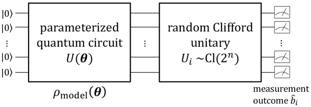
Figure 2: Configuration of the $n$-qubit quantum circuit for training PQC $U(\bm{\theta})$. The PQC is followed by a unitary $U_{i}$, which is selected from the random Clifford unitaries with the size $2^{n}$. Measurement is carried out to obtain the outcome $\hat{b}_{i}$, i.e., a bit string of length $n$.

Here we describe the training method of the PQC for ACAE. The PQC $U(\bm{\theta})$ consists of $n$ qubits and $l$ layers; thus $U(\bm{\theta})$ contains $\mathcal{O}(ln)$ gates. The number of layers $l$ is of the order from $\mathcal{O}(1)$ to $\mathcal{O}(\mbox{poly}(n))$. In this paper we take the PQC composed of single-qubit parameterized rotational gates $R_{x}(\theta_{r})=\exp{(-i\theta_{r}\sigma_{x}/2)}$, $R_{y}(\theta_{r})=\exp{(-i\theta_{r}\sigma_{y}/2)}$, and $R_{z}(\theta_{r})=\exp{(-i\theta_{r}\sigma_{z}/2)}$ together with CNOT gates; here $\theta_{r}$ is the $r$-th element of $\bm{\theta}$ and $\sigma_{x},\sigma_{y},\sigma_{z}$ are the Pauli $X,Y,Z$ operators, respectively. We take the so-called hardware efficient ansatz [34]; an example of the structure is shown in Fig. 1. This PQC is followed by a random Clifford unitary $U_{i}$ as shown in Fig. 2. The output of the circuit is measured $N_{\rm{shot}}$ times in the computational basis, with changing the random Clifford unitary $U_{i}$ and obtaining outcome $\hat{b}_{i}$ in each trial. The above procedure provides us with the classical snapshots of $\rho_{\rm{model}}$. Note that each $\ket{\hat{b_{i}}}$ and $U_{i}$ can be stored efficiently in a classical memory using the stabilizer formalism [32].

Our goal is to find the best $\bm{\theta}$ that maximizes the fidelity $f(\bm{\theta})$. Now we use the classical shadow to have the estimate $\hat{f}(\bm{\theta})$ given in Eq. (10), which can be further calculated as

$$\hat{f}(\bm{\theta}) =\frac{1}{N_{\textrm{shot}}}\sum_{i=1}^{N_{\textrm{shot}}}\textrm{Tr}\left(O\hat{\rho}_{i}(\bm{\theta})\right)$$

$$=\frac{1}{N_{\textrm{shot}}}\sum_{i=1}^{N_{\textrm{shot}}}\textrm{Tr}\left[O\mathcal{M}^{-1}\left(U^{\dagger}_{i}\ket{\hat{b}_{i}}\!\bra{\hat{b}_{i}}U_{i}\right)\right]$$

$$=\frac{1}{N_{\textrm{shot}}}\sum_{i=1}^{N_{\textrm{shot}}}\textrm{Tr}\left[O\left\{(2^{n}+1)U^{\dagger}_{i}\ket{\hat{b}_{i}}\!\bra{\hat{b}_{i}}U_{i}-I\right\}\right]$$

$$=\frac{1}{N_{\textrm{shot}}}\sum_{i=1}^{N_{\textrm{shot}}}(2^{n}+1)\bra{\hat{b}_{i}}U_{i}OU^{\dagger}_{i}\ket{\hat{b}_{i}}-1.$$

Let us consider the run-time for evaluating the above $\hat{f}(\bm{\theta})$ with a classical computer. First, each $\bra{\hat{b}_{i}}U_{i}OU^{\dagger}_{i}\ket{\hat{b}_{i}}$ is calculated as follows;

$$\bra{\hat{b}_{i}}U_{i}OU^{\dagger}_{i}\ket{\hat{b}_{i}} =\bra{\hat{b}_{i}}U_{i}\ket{{\rm Data}}\bra{{\rm Data}}U^{\dagger}_{i}\ket{\hat{b}_{i}}$$

$$=\left|\bra{\hat{b}_{i}}U_{i}\ket{{\rm Data}}\right|^{2}$$

$$=\left|\sum_{k=0}^{N-1}c_{k}\bra{\hat{b}_{i}}U_{i}\ket{k}\right|^{2}.$$ (12)

The Gottesman-Knill theorem [35] allows for evaluation of $\bra{\hat{b}_{i}}U_{i}\ket{k}$ in $\mathcal{O}(n^{2})$-time, because $(\ket{\hat{b}_{i}},\ket{k})$ and $U_{i}$ are stabilizer states and a Clifford operator, respectively. Note that the summation in Eq. (12) requires $\mathcal{O}(N)=\mathcal{O}(2^{n})$ computations, which means that the required run-time in the training process of the PQC scales exponentially with the number of qubit. However, this is classical computation, which should become exponential as long as we would like to process a general exponential-size classical data. Rather, the advantage of ACAE is in the depth of the PQC, which operates only $\mathcal{O}(n\,\mathrm{poly}(n))$ gates instead of $\mathcal{O}(2^{n})$, to achieve $\mathcal{O}(2^{n})$ data encoding.

To maximize the fidelity estimate $\hat{f}(\bm{\theta})$ (i.e., to minimize the $-\hat{f}(\bm{\theta})$), we take the standard gradient descent algorithm. The gradients of $\hat{f}(\bm{\theta})$ with respect to ${\theta}_{r}$ can be computed by using the parameter shift rule [36] as

$$\frac{\partial\hat{f}(\bm{\theta})}{\partial\theta_{r}}=\hat{f}_{{\theta}_{r}}^{+}-\hat{f}_{{\theta}_{r}}^{-},$$ (13)

where

$$\hat{f}_{\theta_{r}}^{\pm}=\hat{f}\left(\theta_{1},\cdots,\theta_{r-1},\theta_{r}\pm\pi/2,\theta_{r+1},\cdots,\theta_{R}\right).$$ (14)

$R$ denotes the number of the parameters, which can be written as $R=ln$ (recall that $l$ is the number of layers of PQC). That is, the gradient can also be effectively estimated using the classical shadow. This maximization procedure will ideally bring us the optimal parameter set $\bm{\theta}^{*}$ and unitary $U(\bm{\theta}^{*})$ that generates a state approximating the target state (2).

III Application To Compact Hadamard Classifier

This section first reviews the method of compact amplitude encoding and the compact Hadamard classifier (CHC). Then we describe how to apply ACAE to implement CHC.

III.1 Compact amplitude encoding

This method encodes two real-valued data vectors into real and imaginary parts of the amplitude of a single quantum state. More specifically, given two $N$-dimensional real-valued vectors $\bm{x}^{+}_{j}=(x_{0j}^{+},\ldots,x_{(N-1)j}^{+})^{T}$ and $\bm{x}^{-}_{j}=(x_{0j}^{-},\ldots,x_{(N-1)j}^{-})^{T}$, the compact amplitude encoder prepares the following quantum state:

$$\ket{\bm{x}_{j}}:=\sum_{l=0}^{N-1}(x_{lj}^{+}+ix^{-}_{lj})\ket{l},$$ (15)

where

$$\|\bm{x}_{j}^{+}\|^{2}+\|\bm{x}^{-}_{j}\|^{2}=1,$$ (16)

is assumed to satisfy the normalization condition. For simplicity, here we assume $\|\bm{x}_{j}^{\pm}\|=1/\sqrt{2}$ without loss of generality. In addition, we define $\ket{\bm{x}^{\pm}_{j}}$ as

$$|\bm{x}_{j}^{\pm}\rangle:=\frac{1}{\|\bm{x}_{j}^{\pm}\|}\sum_{l=0}^{N-1}x_{lj}^{\pm}\ket{l}=\sqrt{2}\sum_{l=0}^{N-1}x_{lj}^{\pm}\ket{l}.$$ (17)

III.2 Compact Hadamard classifier (CHC)

Here we give a quick review about CHC [15]. Suppose the following training data set $\mathcal{D}$ is given;

$$\mathcal{D}=\left\{\left(\bm{x}_{0},y_{0}\right),\ldots,\left(\bm{x}_{M-1},y_{M-1}\right)\right\}.$$

All inputs $\{\bm{x}_{j}\}$ are $N$-dimensional real-valued vectors, and each $y_{j}$ takes either $+1$ or $-1$. The goal of CHC is to predict the label $\tilde{y}$ for a test data $\tilde{\bm{x}}$, which is also a $N$-dimensional real-valued vector. For simplicity, we assume that the number of training data with label $+1$, denoted by $M^{+}$, is equal to the number of training data with label $-1$, denoted by $M^{-}$; i.e., $M^{+}=M^{-}=M/2$ where $M$ is an even number. In particular, we sort the training data set so that

$$\bm{x}_{j}=\begin{cases}\bm{x}_{j}^{+}&\text{($0\leq j\leq M/2-1$)}\\ \bm{x}_{j-M/2}^{-}&\text{($M/2\leq j\leq M-1$)}\\ \end{cases}$$

and

$$y_{j}=\begin{cases}+1&\text{($0\leq j\leq M/2-1$)}\\ -1&\text{($M/2\leq j\leq M-1$)}.\end{cases}$$

Note that CHC can also be applied to imbalanced training data sets as we will see later.

Assuming the existence of the compact amplitude encoder $U_{\mathrm{CAE}}(\bm{x}_{j})$ that encodes the two training data vectors $\bm{x}^{\pm}_{j}$ into a single quantum state (15) and the encoder $U_{\mathrm{AE}}(\bm{\tilde{x}})$ that encodes a test data vector $\tilde{\bm{x}}$ into a quantum state $\ket{\tilde{\bm{x}}}$, the following quantum state can be generated:

$$\ket{\psi_{\mathrm{init}}} =U_{\mathrm{AE}}(\bm{\tilde{x}})U_{\mathrm{CAE}}(\bm{x}_{j})R^{(\rm{A})}_{z}H^{(\rm{A})}U^{(\rm{J})}_{w}(b)\ket{0}_{\rm{A}}\ket{0}_{\rm{D}}\ket{0}_{\rm{J}},$$

$$=U_{\mathrm{AE}}(\bm{\tilde{x}})U_{\mathrm{CAE}}(\bm{x}_{j})\sum_{j=0}^{\frac{M}{2}-1}\sqrt{b_{j}}\frac{\ket{0}_{\rm{A}}+\ket{1}_{\rm{A}}}{\sqrt{2}}\ket{0}_{\rm{D}}\ket{j}_{\rm{J}},$$

$$=\frac{1}{\sqrt{2}}\sum_{j=0}^{\frac{M}{2}-1}\sqrt{b_{j}}\left(\ket{0}_{\rm{A}}\ket{\bm{x}_{j}}_{\rm{D}}+e^{-i\phi}\ket{1}_{\rm{A}}\ket{\tilde{\bm{x}}}_{\rm{D}}\right)\ket{j}_{\rm{J}},$$ (18)

where $\phi$ is the relative phase. Also, ${b_{j}}$ is the set of weights satisfying $\sum_{j=0}^{M/2-1}b_{j}=1$; in this work, we follow Ref. [15] to choose the uniform weighting $b_{j}=2/M$. The labels $``\rm{A}"$, $``\rm{J}"$, and $``\rm{D}"$ mean the ancilla qubit, the qubits for data numbering, and the qubits for data encoding, respectively (the subscript will be omitted unless misunderstood). The number of qubits required to prepare this state is $n+m+1$, where $n=\lceil\log(N)\rceil$ and $m=\lceil\log(M/2)\rceil$. Then, we operate the single-qubit Hadamard gate on the ancilla qubit and have

$$\ket{\psi_{f}}:=H^{(\rm{A})}\ket{\psi_{\mathrm{init}}}= \frac{1}{2}\sum_{j=0}^{\frac{M}{2}-1}\sqrt{b_{j}}\big{[}\ket{0}_{\rm{A}}(\ket{\bm{x}_{j}}_{\rm{D}}+e^{-i\phi}\ket{\tilde{\bm{x}}}_{\rm{D}})$$

$$+\ket{1}_{\rm{A}}(\ket{\bm{x}_{j}}_{\rm{D}}-e^{-i\phi}\ket{\tilde{\bm{x}}}_{\rm{D}})\big{]}\ket{j}_{\rm{J}}.$$ (19)

Finally, we measure the ancilla qubit in the computational basis. The entire quantum circuit is illustrated in Fig. 3.

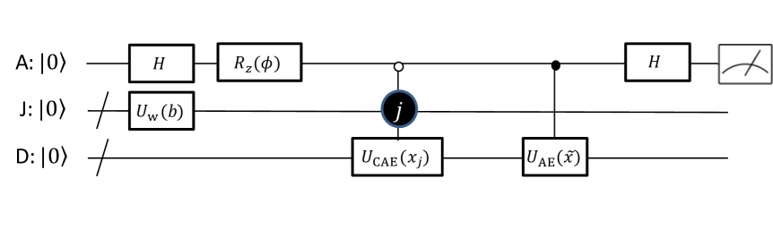
Figure 3: Configuration of the circuit for compact Hadamard classifier. The labels “$\rm{A}$”, “$\rm{J}$”, and “$\rm{D}$” on the left side mean the ancilla qubit, the qubits for data numbering, and the qubits for data encoding, respectively. Slash symbols on the “$\rm{J}$” and “$\rm{D}$” lines indicate that the line is composed of multiple qubits. The number of qubits of the “$\rm{J}$” and “$\rm{D}$” lines are $m=\lceil\log(M/2)\rceil$ and $n=\lceil\log(N)\rceil$, where $M$ and $N$ represent the number of training data and the dimension of the data vector, respectively. $U_{\mathrm{w}}(b)$ is an operator that weights each $\ket{j}$ by ${b_{j}}$. $U_{\mathrm{CAE}}(\bm{x}_{j})$ and $U_{\mathrm{AE}}(\tilde{\bm{x}})$ are the unitary operators that encode the training data $\bm{x}^{\pm}_{j}$ and the test data $\tilde{\bm{x}}$ into $\ket{\bm{x}_{j}}_{\rm{D}}$ and $\ket{\tilde{\bm{x}}}_{\rm{D}}$ in Eq. (18), respectively. The white and black dots connected to $U_{\mathrm{CAE}}(\bm{x}_{j})$ and $U_{\mathrm{AE}}(\tilde{\bm{x}})$ indicate that the control action turns on when the variable takes 1 and 0, respectively. The black circle marked “$\rm{J}$” indicates that the unitary operation $U_{\mathrm{CAE}}(\bm{x}_{j})$ is the uniformly controlled via the “$\rm{J}$” qubits in addition to the “$\rm{A}$” qubit.

Now, the probabilities that the measurement outcome of ancilla qubit is $\ket{0}$ and $\ket{1}$ are given by

$$\Pr(0)=\frac{1}{2}\sum_{j=0}^{\frac{M}{2}-1}b_{j}\left(1+\cos(\phi)\text{Re}(\kappa_{j})-\sin(\phi)\text{Im}(\kappa_{j})\right)$$

and $\Pr(1)=1-\Pr(0)$, where $\kappa_{j}=\langle\tilde{\bm{x}}|\bm{x}_{j}\rangle$. Therefore, the expectation value of the Pauli $Z$ operator measured on the ancilla qubit, denoted as $\sigma_{z}^{(\rm{A})}$, is

$$\langle\sigma_{z}^{(\rm{A})}\rangle=\sum_{j=0}^{M/2-1}b_{j}\left(\cos(\phi)\text{Re}(\kappa_{j})-\sin(\phi)\text{Im}(\kappa_{j})\right).$$

If we set $\phi=\pi/4$, this becomes

$$\langle\sigma_{z}^{(\rm{A})}\rangle=\frac{1}{2}\sum_{j=0}^{\frac{M}{2}-1}b_{j}\left(\langle\tilde{\bm{x}}|\bm{x}_{j}^{+}\rangle-\langle\tilde{\bm{x}}|\bm{x}_{j}^{-}\rangle\right).$$ (20)

Note that, when the number of training data vectors in the two classes are not equal (i.e., $M^{+}\neq M^{-}$), this difference can be compensated by tuning $\phi$ to satisfy $\tan(\phi)=M_{-}/M_{+}$. We now end up with the final form of Eq. (20) as

$$\langle\sigma_{z}^{(\rm{A})}\rangle=\frac{1}{2}\sum_{j=0}^{M-1}b^{\prime}_{j}y_{j}\langle\tilde{\bm{x}}|\bm{x}_{j}\rangle,$$ (21)

where $b^{\prime}_{j}$ is defined as

$$b^{\prime}_{j}=b^{\prime}_{j+M/2}=b_{j},~{}~{}\sum_{j=0}^{M-1}b^{\prime}_{j}=2.$$

Clearly Eq. (21) has the form of standard kernel-based classifier where $\langle\tilde{\bm{x}}|\bm{x}_{j}\rangle$ represents the similarity between the test data $\tilde{\bm{x}}$ and the training data $\bm{x}_{j}$. Because the right-hand side of Eq. (21) represents the sum of the kernel weighted by $b^{\prime}_{j}y_{j}$, the sign of $\langle\sigma_{z}^{(\rm{A})}\rangle$ tells us the class for the test data $\tilde{\bm{x}}$; that is, CHC predicts the label $\tilde{y}$ of $\tilde{\bm{x}}$ via the following policy:

$$\tilde{y}=\text{sgn}\left[\langle\sigma_{z}^{(\rm{A})}\rangle\right]=\text{sgn}\left[\frac{1}{2}\sum_{j=0}^{M-1}b^{\prime}_{j}y_{j}\langle\tilde{\bm{x}}|\bm{x}_{j}\rangle\right].$$ (22)

Note that the weights $\{b_{j}^{\prime}\}$ can be optimized, like the standard kernel-based classifier such as the support vector machine which indeed optimizes those weights depending on the training dataset; this clearly improves the classification performance of ACAE, which will be examined in a future work.

The advantage of quantum kernel-based classifiers over classical classifiers is the accessibility to kernel functions. Actually, the kernel (or similarity) between test data and training data is calculated as the inner product in the feature Hilbert space, which is computationally expensive to evaluate via classical means when the feature space is large. On the other hand, quantum kernel-based classifiers efficiently evaluate kernel functions. In particular, CHC can evaluate the sum of all the inner products in the $N$-dimensional feature space appearing in the right-hand side of Eq. (21), just by measuring the expected value of $\sigma_{z}^{(\rm{A})}$. We also emphasize that CHC can be realized with compact quantum circuits compared with other quantum kernel-based classifiers. Actually, thanks to the compact amplitude encoding, two qubits can be removed in the CHC formulation compared to the others; moreover, the number of operations for encoding the training data set $\bm{x}_{j}$ is reduced by a factor of four compared with HTC [14]. Hence, CHC can be implemented in a compact quantum circuit in both depth and width compared to the other quantum classifiers, meaning that a smaller and thus easier-trainable variational circuit may function for CHC.

III.3 Implementation of CHC using ACAE

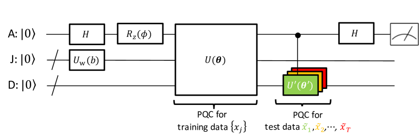
Figure 4: Configuration of the circuit for compact Hadamard classifier using ACAE. We use PQCs instead of the uniformly controlled $U_{\mathrm{CAE}}(\bm{x}_{j})$ and $U_{\mathrm{AE}}(\tilde{\bm{x}})$ in Fig. 3; that is, $U(\bm{\theta})$ represents a PQC for encoding the training data $\{\bm{x}_{j}\}$ and thereby approximately generates $\ket{\bm{x}_{j}}_{\rm{D}}$ in Eq. (III.2). Also, $U^{\prime}(\bm{\theta^{\prime}})$ represents a PQC for encoding the test data $\tilde{\bm{x}}$ and thereby approximately generates $\ket{\tilde{\bm{x}}}_{\rm{D}}$. Note that, in practice, we construct $U(\bm{\theta})$ off-line using all the training data; then we learn $U^{\prime}(\bm{\theta^{\prime}})$ for a given test data $\tilde{\bm{x}}$ for the on-line prediction purpose.

Although CHC efficiently realizes a compact quantum classifier, it relies on the critical assumption; that is, the quantum state (15) is necessarily prepared. Recall that, in general, the quantum circuit for generating the state (15) requires an exponential number of gates. Moreover, to generate the quantum state $\ket{\psi_{\mathrm{init}}}$ in Eq. (18), the uniformly controlled gate [37, 38] shown in Fig. 3 also requires an exponential number of gates. These requirements may destroy the quantum advantage of CHC.

The ACAE implements CHC without using exponentially many gates; that is, as shown below, we can approximately generate the quantum state $\ket{\psi_{f}}$ with a constant-depth quantum circuit illustrated in Fig. 4. First, by applying $H,R_{z}(\phi)$, and $U_{w}(b)$ on the initial states, we produce the following state:

$$\ket{\psi_{0}}:=\frac{1}{\sqrt{2}}\sum_{j=0}^{\frac{M}{2}-1}\sqrt{b_{j}}\left(\ket{0}_{\rm{A}}\ket{0}_{\rm{D}}+e^{-i\phi}\ket{1}_{\rm{A}}\ket{0}_{\rm{D}}\right)\ket{j}_{\rm{J}}.$$ (23)

Next, we train $U(\bm{\theta})$ by the algorithm described in Section II, so that it approximately encodes the training data $\{\bm{x}_{j}\}$ to have

$$\ket{\psi_{1}} :=U(\bm{\theta})\ket{\psi_{0}}$$

$$\approx e^{i\alpha}\frac{1}{\sqrt{2}}\sum_{j=0}^{\frac{M}{2}-1}\sqrt{b_{j}}\left(\ket{0}_{\rm{A}}\ket{\bm{x}_{j}}_{\rm{D}}+e^{-i\phi}\ket{1}_{\rm{A}}\ket{0}_{\rm{D}}\right)\ket{j}_{\rm{J}},$$ (24)

where $e^{i\alpha}$ is the global phase. We then set the controlled $U^{\prime}(\bm{\theta^{\prime}})$ to encode the test data $\tilde{\bm{x}}$ to obtain

$$(\ket{0}_{\rm{A}}\bra{0}_{\rm{A}}\otimes I+\ket{1}_{\rm{A}}\bra{1}_{\rm{A}}\otimes U^{\prime}(\bm{\theta^{\prime}}))\ket{\psi_{1}}$$

$$\approx e^{i\alpha}\frac{1}{\sqrt{2}}\sum_{j=0}^{\frac{M}{2}-1}\sqrt{b_{j}}\left(\ket{0}_{\rm{A}}\ket{\bm{x}_{j}}_{\rm{D}}+e^{-i\phi}\ket{1}_{\rm{A}}\ket{\tilde{\bm{x}}}_{\rm{D}}\right)\ket{j}_{\rm{J}}$$

$$=e^{i\alpha}\ket{\psi_{\mathrm{init}}}.$$ (25)

Finally, we operate $H$ on the ancilla qubit to obtain $\ket{\psi_{f}}$;

$$H^{(\rm{A})}e^{i\alpha}\ket{\psi_{\mathrm{init}}}=e^{i\alpha}\ket{\psi_{f}}.$$ (26)

Although the global phase $e^{i\alpha}$ is added to $\ket{\psi_{f}}$, this does not affect the probability $\Pr(0)$ and the expectation value $\langle\sigma_{z}^{(\rm{A})}\rangle$. Recall that, $U(\bm{\theta})$ and $U^{\prime}(\bm{\theta^{\prime}})$ consist of $(n+m+1)$ qubits with $\mathcal{O}(1)\sim\mathcal{O}(\mbox{poly}(n+m+1))$ layers and $n$ qubits with $\mathcal{O}(1)\sim\mathcal{O}(\mbox{poly}(n))$ layers, respectively. Therefore, we can implement the approximated CHC without using exponentially many gates.

Before moving forward, we give some remarks, regarding the design of $U^{\prime}(\bm{\theta^{\prime}})$. First, we assume that $U^{\prime}(\bm{\theta^{\prime}})$ consists of only $R_{y}$ gates and CNOT gates, because $\tilde{\bm{x}}$ is a real-valued data vector. As a result, the unitary process is restricted to $U^{\prime}(\bm{\theta^{\prime}})\ket{0}_{\rm{D}}\approx\pm\ket{\tilde{\bm{x}}}_{\rm{D}}$, which is further converted to $U^{\prime}(\bm{\theta^{\prime}})\ket{0}_{\rm{D}}\approx\ket{\tilde{\bm{x}}}_{\rm{D}}$ by compensating the phase via the choice of $\phi$ in Eq. (25). Next, to implement the controlled $U^{\prime}(\bm{\theta^{\prime}})$, every elementary gate contained in $U^{\prime}(\bm{\theta^{\prime}})$ has to be modified to a controlled-gate via the “$\rm{A}$” qubit. Finally, in practice, we construct $U(\bm{\theta})$ off-line using all the training data; once a test data $\tilde{\bm{x}}$ to be classified is given to us, then we learn $U^{\prime}(\bm{\theta^{\prime}})$ to approximately encode $\tilde{\bm{x}}$ and then construct CHC to predict the corresponding label $\tilde{y}$.

IV Demonstration

Table 1: The data contents embedded in the quantum amplitude of $\ket{\psi_{\mathrm{init}}}$ in Iris setosa and Iris versicolor classification problem. The “$\rm{A}$”, “$\rm{J}$”, and “$\rm{D}$” in the left three columns represent the ancilla qubit, the qubits for data numbering, and the qubits for data encoding, respectively, as in Fig. 3. The “$i$” in the right end column represents an imaginary unit. The amplitudes are normalized to satisfy Eq. (16).

$``\rm{A}"$	$``\rm{J}"$	$``\rm{D}"$	basis	data contents embedded in the amplitude of each basis
ancilla qubit	qubits for	qubits for
0 : training data	data numbering	data enconding
1 : test data	(from 0 to $M/2$)	(from 0 to $M$)
0	00	00	$\ket{00000}$	(1st feature of Iris setosa) + (1st feature of Iris versicolor)$\times i$
		01	$\ket{00001}$	(2nd feature of Iris setosa) + (2nd feature of Iris versicolor)$\times i$
		10	$\ket{00010}$	(3rd feature of Iris setosa) + (3rd feature of Iris versicolor)$\times i$
		11	$\ket{00011}$	(4th feature of Iris setosa) + (4th feature of Iris versicolor)$\times i$
	$\vdots$	$\vdots$	$\vdots$	$\vdots$
	11	00	$\ket{01100}$	(1st feature of Iris setosa) + (1st feature of Iris versicolor)$\times i$
		01	$\ket{01101}$	(2nd feature of Iris setosa) + (2nd feature of Iris versicolor)$\times i$
		10	$\ket{01110}$	(3rd feature of Iris setosa) + (3rd feature of Iris versicolor)$\times i$
		11	$\ket{01111}$	(4th feature of Iris setosa) + (4th feature of Iris versicolor)$\times i$
1	00	00	$\ket{10000}$	(1st feature of the test data)$\times\exp(-i\phi)$
		01	$\ket{10001}$	(2nd feature of the test data)$\times\exp(-i\phi)$
		10	$\ket{10010}$	(3rd feature of the test data)$\times\exp(-i\phi)$
		11	$\ket{10011}$	(4th feature of the test data)$\times\exp(-i\phi)$
	$\vdots$	$\vdots$	$\vdots$	$\vdots$
	11	00	$\ket{11100}$	(1st feature of the test data)$\times\exp(-i\phi)$
		01	$\ket{11101}$	(2nd feature of the test data)$\times\exp(-i\phi)$
		10	$\ket{11110}$	(3rd feature of the test data)$\times\exp(-i\phi)$
		11	$\ket{11111}$	(4th feature of the test data)$\times\exp(-i\phi)$

This section gives two numerical demonstrations to show the performance of our algorithm composed of ACAE and CHC. First we present an example application to a classification problem for the Iris dataset [39]. Next we show application to the fraud detection problem using the credit card fraud dataset [40] provided in Kaggle.

IV.1 Iris dataset classification

The Iris dataset consists of three iris species (Iris setosa, Iris virginica, and Iris versicolor) with 50 samples each as well as four features (sepal length, sepal width, petal length, and petal width) for each flower. Each sample data includes ID number, four features, and species. IDs for 1 to 50, 51 to 100, and 101 to 150 represent data for Iris setosa, Iris versicolor, and Iris virginica, respectively.

In this paper, we consider the Iris setosa and Iris versicolor classification problem. The goal is to create a binary classifier that predicts the correct label $\tilde{y}$ (0 : Iris setosa, 1 : Iris versicolor) for given test data $\tilde{\bm{x}}=$(sepal length, sepal width, petal length, petal width). In this demonstration, we employ the first four data of each species as training data. That is, we use data with IDs 1 to 4 and 51 to 54 as training data for Iris setosa and Iris versicolor, respectively. On the other hand, we use data with IDs 5 to 8 and 55 to 58 as test data.

First, we need to prepare the quantum state $\ket{\psi_{\mathrm{init}}}$ given in Eq. (18) using ACAE. Since the dimension of the feature vector and the number of training data are $N=4$ and $M=8$, the number of required qubits are $n=\lceil\log(N)\rceil=2$ and $m=\lceil\log(M/2)\rceil=2$, respectively. The number of total qubits required for composing the quantum circuit is $n+m+1=5$, which means that $\ket{\psi_{\mathrm{init}}}$ has $2^{5}=32$ amplitudes. TABLE 1 shows the data contents embedded in the quantum amplitude of each basis.

We encode the training data of the Iris setosa and Iris versicolor into the complex amplitude of the ancilla qubit state $\ket{0}$ by using the PQC $U(\bm{\theta})$. Also, we encode the test data into the amplitude of the ancilla qubit state $\ket{1}$ by using $U^{\prime}(\bm{\theta^{\prime}})$. We use the 5-qubit and 12-layer ansatz $U(\bm{\theta})$ illustrated in Fig. 1. We randomly initialize all the direction of each rotating gate (i.e., $X,Y$, or $Z$) and $\theta_{r}$ at the beginning of each training. As the optimizer, Adam [41] is used. The number of iterations (i.e., the number of the updates of the parameters) is set to $400$ for training $U(\bm{\theta})$. For each iteration, 1000 classical snapshots are used to estimate the fidelity; that is, we set $N_{\textrm{shot}}=1000$ in Eq. (8). The learning rate is 0.1 for the first $100$ iterations, 0.01 for the next $100$ iterations, 0.005 for the next $100$ iterations, and 0.001 for the last $100$ iterations. In Fig. 5, we show the change of fidelity in the training process of $U(\bm{\theta})$. At the end of the training, the fidelity reaches 0.994.

As for the encoding process of test data, we use the 2-qubit and 2-layer ansatz $U^{\prime}(\bm{\theta^{\prime}})$ that consists of only $R_{y}$ gates and CNOT gates. The number of iterations and $N_{\textrm{shot}}$ are $100$ and $1000$, respectively. The learning rate is 0.1 for the first $50$ iterations and 0.01 for the next $50$. We found that, for each test data, the fidelity reaches the value bigger than 0.999. It is notable that the number of layers of $U^{\prime}(\bm{\theta^{\prime}})$ and the number of iterations for training it are much smaller compared to the encoding process for training data. This means, once the training data is encoded, it is easy to change the test data.

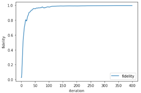
Figure 5: The change of the fidelity between the target state and the model state in the training process of $U(\bm{\theta})$. Here, the target state is (III.3), and the model state means the state that is actually generated by the PQC $U(\bm{\theta})$.

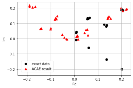
(a) The complex amplitudes of $\ket{\psi_{\mathrm{init}}}$ generated by ACAE (red triangles) and exact data (black dots). Note that red dots contain influence of the global phase $e^{i\alpha}$.

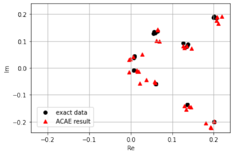
(b) The result in which the global phase is hypothetically eliminated is shown. The fidelity between model state (red triangles) and target state (black dots) is 0.993.

Figure 6: An example of data encoding results. Note that each data value is divided by a constant number to satisfy the normalization condition (16).

As an example of the data encoding results, a set of complex amplitudes generated by ACAE is shown in Fig. 6. In the figure, the value of each complex amplitude is plotted on the complex plane. The black dots and red triangles represent the exact data and the approximate complex amplitudes embedded by ACAE, respectively. Note that the complex amplitude embedded by ACAE contains a global phase $e^{i\alpha}$ as in Eq. (25). In order to compare the exact data with the ACAE result visually, the result in which the global phase is hypothetically eliminated is also shown. Recall that the global phase does not affect the measurement in the remaining procedure.

After the state preparation, we operate the Hadamard gate on the ancilla qubit and obtain $\ket{\psi_{f}}$ in Eq. (III.2). By measuring the ancilla qubit of this quantum state and obtaining the sign of $\langle\sigma_{z}^{(\rm{A})}\rangle$, we can use Eq. (22) to predict the label $\tilde{y}$ of the test data $\tilde{\bm{x}}$, i.e., $\tilde{y}=\text{sgn}\left[\langle\sigma_{z}^{(\rm{A})}\rangle\right]$. Classification results are shown in TABLE 3(a) for 8 cases in which test data are IDs 5 to 8 and IDs 55 to 58. In addition to the Iris setosa and Iris versicolor classification problem, we carry out Iris versicolor and Iris virginica classification problem in the same way and show the result in TABLE 3(b). All classification results are correct in TABLE 3(a). On the other hand, three out of eight classification results are incorrect in TABLE 3(b).

Let us discuss the results. Pairwise relationships in Iris dataset shows that Iris setosa can be clearly separated from the other two varieties, whereas the features of Iris versicolor and Iris virginica slightly overlap with each other. Therefore, classification of Iris versicolor and Iris virginica (TABLE 3(b)) is considered more difficult than that of Iris setosa and Iris versicolor (TABLE 3(a)). This could be the cause of the low accuracy rate of TABLE 3(b). Note that the error between the exact data and ACAE data also affects on the classification accuracy. If we adjust the number of layers in the PQC and the number of iterations in the training process to improve the fidelity between the target state and the model state, we will be able to increase the accuracy rate. In fact, we confirmed that the incorrect results (#55, #56, #57) turned correct when the classifications are performed using the exact data. Table 3(c) shows the results where both the training and test data are ideally encoded without errors.

Table 2: The results of the Iris dataset classification problem

test data ID	class	$\quad\langle\sigma_{z}^{(\rm{A})}\rangle\quad$	$\quad\tilde{y}\quad$	result
#5		0.0422	$+$	Correct
#6	Iris setosa	0.0364	$+$	Correct
#7	($+$)	0.0395	$+$	Correct
#8		0.0374	$+$	Correct
#55		-0.0317	$-$	Correct
#56	Iris versicolor	-0.0315	$-$	Correct
#57	($-$)	-0.0285	$-$	Correct
#58		-0.0239	$-$	Correct

(a) Iris setosa versus Iris versicolor

test data ID	class	$\quad\langle\sigma_{z}^{(\rm{A})}\rangle\quad$	$\quad\tilde{y}\quad$	result
#55		-0.0001	$-$	Incorrect
#56	Iris versicolor	-0.0015	$-$	Incorrect
#57	$(+)$	-0.0020	$-$	Incorrect
#58		0.0010	$+$	Correct
#105		-0.0083	$-$	Correct
#106	Iris virginica	-0.0066	$-$	Correct
#107	$(-)$	-0.0089	$-$	Correct
#108		-0.0054	$-$	Correct

(b) Iris versicolor versus Iris virginica

test data ID	class	$\quad\langle\sigma_{z}^{(\rm{A})}\rangle\quad$	$\quad\tilde{y}\quad$	result
#55		0.0322	$+$	Correct
#56	Iris versicolor	0.0013	$+$	Correct
#57	$(+)$	0.0230	$+$	Correct
#58		0.0534	$+$	Correct
#105		-0.0392	$-$	Correct
#106	Iris virginica	-0.0269	$-$	Correct
#107	$(-)$	-0.0430	$-$	Correct
#108		-0.0194	$-$	Correct

(c) Iris versicolor versus Iris virginica (Exact data are used.)

IV.2 Credit cards fraud detection

Nowadays, credit card fraud is a social problem in terms of customer protection, financial crime prevention, and avoiding negative impacts on corporate finances. The losses that arise from credit card fraud are a serious problem for financial institutions; according to the Nilson Report [42], credit card fraud losses are expected to reach $49.3 billion by 2030. Banks and credit card companies that pay for fraud will be hit hard by these rising costs. With digital crime and online fraud on the rise, it is more important than ever for financial institutions to prevent credit card fraud through advanced technology and strong security measures. To detect fraudulent use, financial institutions use human judgment to determine fraud based on information such as cardholder attributes, past transactions, and product delivery address information, however this method requires human resources and costs. Although attempts to detect fraud by machine learning based on features extracted from credit card transaction data also have been attracting attention in recent years, there are disadvantages such as more time and epochs to converge for a stable prediction, excessive training and so on. Quantum machine learning has the potential to solve these challenges, and its application to credit card fraud detection deserve exploring.

In this subsection, we demonstrate credit card fraud detection as another practical application of CHC with ACAE. The goal is to encode credit card transaction data into a quantum state as training data and classify whether a given transaction data $\tilde{\bm{x}}$ is a normal ($\tilde{y}=+1$) or fraudulent transaction ($\tilde{y}=-1$).

In this demonstration we use the credit card fraud detection dataset [40] provided by Kaggle. The dataset contains credit card transactions made by European cardholders in September 2013. The dataset has 284,807 transactions which include 492 fraudulent transactions. Note that, since it is difficult to encode all transaction data into a quantum state, for proof-of-concept testing, we take 4 normal transaction data and 4 fraudulent transaction data from this dataset as training data, and perform classification tests to determine whether given test data is normal or fraudulent. Each data consists of Times, Amount and 28 different features ($V1,V2,\dots,V28$) transformed by principal component analysis. We use 4 features ($V1,V2,V3,V4$) out of the 28 features for classification, which means that the dimension of the feature vector and the number of training data are $N=4$ and $M=8$ respectively, and the number of total qubits required for composing quantum circuit is $n+m+1=5$. As in the previous subsection, we embed the training data of normal transaction and fraudulent transaction into the real and imaginary parts of the complex amplitude of the ancilla qubit state $\ket{0}$ and embed the test data into the complex amplitude of the ancilla qubit state $\ket{1}$.

After the state preparation, we operate the Hadamard gate on the ancilla qubit and make measurements to obtain $\langle\sigma_{z}^{(\rm{A})}\rangle$ the sign of which provides classification result, i.e., $\tilde{y}=+1$ for normal data and $\tilde{y}=-1$ for fraudulent data. As test data, we take the top four normal data ID and fraudulent data ID, in ascending order, excluding the training data. Classification results are shown in TABLE 3.

Table 3: The results of fraud detection.

[h] test data ID¹ class $\quad\langle\sigma_{z}^{(\rm{A})}\rangle\quad$ $\quad\tilde{y}\quad$    result #5 0.0699 $+$ Correct #6 normal 0.1978 $+$ Correct #7 ($+$) 0.0183 $+$ Correct #8 0.1579 $+$ Correct #6330 -0.3747 $-$ Correct #6332 fraud -0.4245 $-$ Correct #6335 ($-$) -0.4289 $-$ Correct #6337 -0.4163 $-$ Correct

• As test data, we take the top four normal data ID and fraudulent data ID, in ascending order, excluding the training data.

V Conclusion

In this paper, we proposed the approximate complex amplitude encoding algorithm (ACAE) which allows for the efficient encoding of given complex-valued classical data into quantum states using shallow parameterized quantum circuits. The key idea of this algorithm is to use the fidelity as a cost function, which can reflect the difference in complex amplitude between the model state and the target state, unlike the MMD-based cost function in the original AAE. Also note that the classical shadow with random Clifford unitary is used for efficient fidelity estimation. In addition, we applied ACAE to realize CHC with fewer gates than the original CHC which requires an exponential number of gates to prepare the exact quantum state. Using this algorithm we demonstrated Iris data classification and the credit card fraud detection that is considered as a key challenge in financial institutions.

For practical applications of ACAE, we need to deal with enormously large dataset. For example, in the demonstration for credit card fraud detection, approximately 280,000 training data are provided and each data has 28 different features. This means $n+m+1=\lceil\log(28)\rceil+\lceil\log(280,000/2)\rceil+1=23$ qubits are required to deal with the whole data. As the number of qubits is increased, the degree of freedom of the quantum state exponentially grows; in such case, there appear several practical problems to be resolved. For example, ACAE employs the fidelity as a cost function, which is however known as a global cost that leads to the so-called gradient vanishing problem or the barren plateau problem [43]; i.e., the gradient vector of the cost decays exponentially fast with respect to the number of qubits, and thus the learning process becomes completely stuck for large-size systems. To mitigate this problem, recently the localized fidelity measurement has been proposed in Refs. [44, 45, 46]. Moreover, applications of several existing methods such as circuit initialization [47, 48], special structured ansatz [49, 50], and parameter embedding [51] are worth investigating to address the gradient vanishing problem. Another problem from a different perspective is that the random Clifford measurement for producing the classical shadow can be challenging to implement in practice, because $\mathcal{O}\left(n^{2}/\log(n)\right)$ entangling gates are needed to sample from $n$-qubit Clifford unitaries. Refs. [52, 53] presented that Clifford circuit depth over unrestricted architectures is upper bounded by $2n+\mathcal{O}\left(\log^{2}(n)\right)$ for all practical purposes, which may improve the implementation of the fidelity estimation process. Overall, algorithm improvements to deal with these problems are all important and remain as future works.

References

- [1] P. Wittek. Quantum machine learning: what quantum computing means to data mining. Academic Press, 2014.
- [2] J. Biamonte, P. Wittek, N. Pancotti, P. Rebentrost, N. Wiebe and S. Lloyd. Quantum machine learning. Nature, 549(7671):195–202, 2017.
- [3] M. Schuld and F. Petruccione. Supervised learning with quantum computers, volume 17. Springer, 2018.
- [4] V. Dunjko and H. J. Briegel. Machine learning & artificial intelligence in the quantum domain: a review of recent progress. Reports on Progress in Physics, 81(7):074001, 2018.
- [5] C. Ciliberto, M. Herbster, A. D. Ialongo, M. Pontil, A. Rocchetto, S. Severini and L. Wossnig. Quantum machine learning: a classical perspective. Proceedings of the Royal Society A: Mathematical, Physical and Engineering Sciences, 474(2209):20170551, 2018.
- [6] M. Schuld. Supervised quantum machine learning models are kernel methods. arXiv preprint arXiv:2101.11020, 2021.
- [7] V. Giovannetti, S. Lloyd and L. Maccone. Quantum random access memory. Physical review letters, 100(16):160501, 2008.
- [8] D. K. Park, F. Petruccione and J.-K. K. Rhee. Circuit-based quantum random access memory for classical data. Scientific reports, 9(1):1–8, 2019.
- [9] T. M. De Veras, I. C. De Araujo, D. K. Park and A. J. Da Silva. Circuit-based quantum random access memory for classical data with continuous amplitudes. IEEE Transactions on Computers, 70(12):2125–2135, 2020.
- [10] A. W. Harrow, A. Hassidim and S. Lloyd. Quantum algorithm for linear systems of equations. Physical review letters, 103(15):150502, 2009.
- [11] P. Rebentrost, M. Mohseni and S. Lloyd. Quantum support vector machine for big data classification. Physical review letters, 113(13):130503, 2014.
- [12] S. Lloyd, M. Mohseni and P. Rebentrost. Quantum principal component analysis. Nature Physics, 10(9):631–633, 2014.
- [13] C. Blank, D. K. Park, J.-K. K. Rhee and F. Petruccione. Quantum classifier with tailored quantum kernel. npj Quantum Information, 6(1):1–7, 2020.
- [14] M. Schuld, M. Fingerhuth and F. Petruccione. Implementing a distance-based classifier with a quantum interference circuit. EPL (Europhysics Letters), 119(6):60002, 2017.
- [15] C. Blank, A. J. da Silva, L. P. de Albuquerque, F. Petruccione and D. K. Park. Compact quantum kernel-based binary classifier. Quantum Science and Technology, 7(4):045007, 2022.
- [16] D. K. Park, C. Blank and F. Petruccione. The theory of the quantum kernel-based binary classifier. Physics Letters A, 384(21):126422, 2020.
- [17] L. K. Grover. Synthesis of quantum superpositions by quantum computation. Physical review letters, 85(6):1334, 2000.
- [18] Y. R. Sanders, G. H. Low, A. Scherer and D. W. Berry. Black-box quantum state preparation without arithmetic. Physical review letters, 122(2):020502, 2019.
- [19] M. Plesch and Č. Brukner. Quantum-state preparation with universal gate decompositions. Physical Review A, 83(3):032302, 2011.
- [20] V. V. Shende, S. S. Bullock and I. L. Markov. Synthesis of quantum logic circuits. In Proceedings of the 2005 Asia and South Pacific Design Automation Conference, pages 272–275, 2005.
- [21] L. Grover and T. Rudolph. Creating superpositions that correspond to efficiently integrable probability distributions. arXiv preprint quant-ph/0208112, 2002.
- [22] M. Möttönen, J. J. Vartiainen, V. Bergholm and M. M. Salomaa. Quantum circuits for general multiqubit gates. Physical review letters, 93(13):130502, 2004.
- [23] V. V. Shende and I. L. Markov. Quantum circuits for incompletely specified two-qubit operators. arXiv preprint quant-ph/0401162, 2004.
- [24] K. Nakaji, S. Uno, Y. Suzuki, R. Raymond, T. Onodera, T. Tanaka, H. Tezuka, N. Mitsuda and N. Yamamoto. Approximate amplitude encoding in shallow parameterized quantum circuits and its application to financial market indicators. Phys. Rev. Research, 4:023136, 2022.
- [25] P. J. Ollitrault, G. Mazzola and I. Tavernelli. Nonadiabatic molecular quantum dynamics with quantum computers. Physical Review Letters, 125(26):260511, 2020.
- [26] H. H. S. Chan, R. Meister, T. Jones, D. P. Tew and S. C. Benjamin. Grid-based methods for chemistry modelling on a quantum computer. arXiv preprint arXiv:2202.05864, 2022.
- [27] J.-G. Liu and L. Wang. Differentiable learning of quantum circuit Born machines. Physical Review A, 98(6):062324, 2018.
- [28] B. Coyle, D. Mills, V. Danos and E. Kashefi. The Born supremacy: Quantum advantage and training of an ising Born machine. npj Quantum Information, 6(1):1–11, 2020.
- [29] H.-Y. Huang, R. Kueng and J. Preskill. Predicting many properties of a quantum system from very few measurements. Nature Physics, 16:1050–1057, 2020.
- [30] G. M. D’Ariano, M. G. Paris and M. F. Sacchi. Quantum tomography. Advances in Imaging and Electron Physics, 128:206–309, 2003.
- [31] S. Hillmich, C. Hadfield, R. Raymond, A. Mezzacapo and R. Wille. Decision diagrams for quantum measurements with shallow circuits. In 2021 IEEE International Conference on Quantum Computing and Engineering (QCE), pages 24–34. IEEE, 2021.
- [32] S. Aaronson and D. Gottesman. Improved simulation of stabilizer circuits. Physical Review A, 70(5):052328, 2004.
- [33] K. N. Patel, I. L. Markov and J. P. Hayes. Optimal synthesis of linear reversible circuits. Quantum Inf. Comput., 8(3):282–294, 2008.
- [34] A. Kandala, A. Mezzacapo, K. Temme, M. Takita, M. Brink, J. M. Chow and J. M. Gambetta. Hardware-efficient variational quantum eigensolver for small molecules and quantum magnets. Nature, 549(7671):242–246, 2017.
- [35] D. Gottesman. The heisenberg representation of quantum computers. arXiv preprint quant-ph/9807006, 1998.
- [36] G. E. Crooks. Gradients of parameterized quantum gates using the parameter-shift rule and gate decomposition. arXiv preprint arXiv:1905.13311, 2019.
- [37] M. Mottonen, J. J. Vartiainen, V. Bergholm and M. M. Salomaa. Transformation of quantum states using uniformly controlled rotations. arXiv preprint quant-ph/0407010, 2004.
- [38] V. Bergholm, J. J. Vartiainen, M. Möttönen and M. M. Salomaa. Quantum circuits with uniformly controlled one-qubit gates. Physical Review A, 71(5):052330, 2005.
- [39] Iris species. https://www.kaggle.com/datasets/uciml/iris.
- [40] Credit card fraud detection. https://www.kaggle.com/datasets/mlg-ulb/creditcardfraud.
- [41] D. P. Kingma and J. Ba. Adam: A method for stochastic optimization. arXiv:1412.6980, 2014.
- [42] Nilson report, 2021. https://nilsonreport.com/upload/content_promo/NilsonReport_Issue1209.pdf.
- [43] J. R. McClean, S. Boixo, V. N. Smelyanskiy, R. Babbush and H. Neven. Barren plateaus in quantum neural network training landscapes. Nature communications, 9(1):1–6, 2018.
- [44] S. Khatri, R. LaRose, A. Poremba, L. Cincio, A. T. Sornborger and P. J. Coles. Quantum-assisted quantum compiling. Quantum, 3:140, 2019.
- [45] K. Sharma, S. Khatri, M. Cerezo and P. J. Coles. Noise resilience of variational quantum compiling. New Journal of Physics, 22(4):043006, 2020.
- [46] H. Tezuka, S. Uno and N. Yamamoto. Generative model for learning quantum ensemble via optimal transport loss. arXiv preprint arXiv:2210.10743, 2022.
- [47] E. Grant, L. Wossnig, M. Ostaszewski and M. Benedetti. An initialization strategy for addressing barren plateaus in parametrized quantum circuits. Quantum, 3:214, 2019.
- [48] K. Zhang, M.-H. Hsieh, L. Liu and D. Tao. Gaussian initializations help deep variational quantum circuits escape from the barren plateau. arXiv preprint arXiv:2203.09376, 2022.
- [49] M. Cerezo, A. Sone, T. Volkoff, L. Cincio and P. J. Coles. Cost function dependent barren plateaus in shallow parametrized quantum circuits. Nature communications, 12(1):1–12, 2021.
- [50] X. Liu, G. Liu, J. Huang and X. Wang. Mitigating barren plateaus of variational quantum eigensolvers. arXiv preprint arXiv:2205.13539, 2022.
- [51] T. Volkoff and P. J. Coles. Large gradients via correlation in random parameterized quantum circuits. Quantum Science and Technology, 6(2):025008, 2021.
- [52] D. Maslov and B. Zindorf. Depth optimization of CZ, CNOT, and Clifford circuits. IEEE Transactions on Quantum Engineering, 2022.
- [53] D. Maslov and W. Yang. CNOT circuits need little help to implement arbitrary hadamard-free clifford transformations they generate, 2022.