Underdetermined Dyson-Schwinger equations

Abstract

This paper examines the effectiveness of the Dyson-Schwinger (DS) equations as a calculational tool in quantum field theory. The DS equations are an infinite sequence of coupled equations that are satisfied exactly by the connected Green’s functions $G_{n}$ of the field theory. These equations link lower to higher Green’s functions and, if they are truncated, the resulting finite system of equations is underdetermined. The simplest way to solve the underdetermined system is to set all higher Green’s function(s) to zero and then to solve the resulting determined system for the first few Green’s functions. The $G_{1}$ or $G_{2}$ so obtained can be compared with exact results in solvable models to see if the accuracy improves for high-order truncations. Five $D=0$ models are studied: Hermitian $\phi^{4}$ and $\phi^{6}$ and non-Hermitian $i\phi^{3}$, $-\phi^{4}$, and $i\phi^{5}$ theories. The truncated DS equations give a sequence of approximants that converge slowly to a limiting value but this limiting value always differs from the exact value by a few percent. More sophisticated truncation schemes based on mean-field-like approximations do not fix this formidable calculational problem.

The objective in quantum field theory is to calculate connected Green’s functions $G_{n}(x_{1},...x_{n})$, which contain the physical content of the theory. In principle, the program is to solve the field equations for the field $\phi(x)$ and then to calculate vacuum expectation values (VEVs) of time-ordered products of $\phi$: $\gamma_{n}(x_{1},...x_{n})\equiv\langle 0|{\rm T}\{\phi(x_{1})...\phi(x_{n})\}|0\rangle.$ The nonconnected Green’s functions $\gamma_{n}$ are then combined into cumulants to get $G_{n}$ r1 .

The Dyson-Schwinger (DS) equations purport to be a way to calculate both the perturbative and nonperturbative behavior of $G_{n}$ by using c-number functional analysis without resorting to operator theory coleman ; r2 ; r3 ; r4 . The procedure is to truncate the infinite system of coupled DS equations to a finite set of coupled equations that would give good approximations to the first few $G_{n}$. The problem is that, while the DS equations are satisfied exactly by $G_{n}$, the DS equations are an underdetermined system; each new equation introduces additional Green’s functions, so a truncation of the system contains more Green’s functions than equations oldpaper . A plausible strategy is to close the truncated system by setting the highest Green’s function(s) to zero and then to solve the resulting determined system.

Here we study the simplest case: quantum field theory in zero-dimensional spacetime. Successive elimination gives polynomial equations for $G_{1}$ or $G_{2}$. We examine the convergence and accuracy of this procedure as the system of coupled equations increases in size for five $D=0$ theories, Hermitian quartic and sextic theories and non-Hermitian $\mathcal{PT}$-symmetric cubic, quartic, and quintic theories r5 . The truncated DS equations provide fair numerical values for the connected Green’s functions, but these approximations do not converge to the exact results when they are examined in high order.

The DS equations follow directly on differentiating the functional integral for $Z[J]$ (or $\log(Z[J])$) with respect to $J$, giving $\gamma_{n}$ (or $G_{n}$),

$$Z[J]=\textstyle{\int\mathcal{D}\phi\,\exp\int dx}\{-\mathcal{L}[\phi(x)]+J(x)\phi(x)\},$$

where $\mathcal{L}$ is the Lagrangian, $J$ is a c-number source, and $Z[0]$ is the Euclidean partition function bms ; r7 .

Hermitian quartic $D=0$ theory: The functional integral $Z[J]$ becomes an ordinary integral $Z[J]=\int_{-\infty}^{\infty}d\phi\,e^{-\mathcal{L}(\phi)}$, where $\mathcal{L}(\phi)=\mbox{$\textstyle{\frac{1}{4}}$}\phi^{4}-J\phi$. The exact connected two-point Green’s function is:

$$G_{2} = \textstyle{\int_{-\infty}^{\infty}}d\phi\,\phi^{2}e^{-\phi^{4}/4}\big{/}\textstyle{\int_{-\infty}^{\infty}}d\phi\,e^{-\phi^{4}/4}$$ (1)

$$= 2\Gamma\big{(}\mbox{$\textstyle{\frac{3}{4}}$}\big{)}\big{/}\Gamma\big{(}\mbox{$\textstyle{\frac{1}{4}}$}\big{)}=0.675\,978\,240...\,.$$

We impose parity invariance when $J=0$, so all odd Green’s functions vanish. The first nontrivial DS equation reads $G_{4}=-3G_{2}^{2}+1$. Truncating this equation by setting $G_{4}=0$, we obtain the approximate result $G_{2}=1/\sqrt{3}=0.577\,350...\,$. In comparison with (1), this result is 14.6% low, which is unimpressive.

The next three DS equations are

$$G_{6}\! = \!-12G_{2}G_{4}-6G_{2}^{3},$$

$$G_{8}\! = \!-18G_{2}G_{6}-30G_{4}^{2}-60G_{2}^{2}G_{4},$$ (2)

$$G_{10}\! = \!-24G_{2}G_{8}-168G_{4}G_{6}-126G_{2}^{2}G_{6}-420G_{2}G_{4}^{2}.$$

This system is underdetermined; the number of unknowns is always one more than the number of equations. To solve this system we eliminate $G_{4}$ by substituting the first equation into the second, we eliminate $G_{6}$ by substituting the first two equations into the third, and so on. We obtain $G_{2n}$ as an $n$th degree polynomial $P_{n}(G_{2})$ (dividing by the coefficient of the highest power of $G_{2}$):

$$\!\!\!\!\!\!P_{2}(x)=x^{2}-\mbox{$\textstyle{\frac{1}{3}}$},\leavevmode\nobreak\ P_{3}(x)=x^{3}-\textstyle{\frac{2}{5}}x,$$

$$\!\!\!\!\!\!P_{4}(x)=x^{4}-\textstyle{\frac{8}{15}}x^{2}+\textstyle{\frac{1}{21}},\leavevmode\nobreak\ P_{5}(x)=x^{5}-\mbox{$\textstyle{\frac{2}{3}}$}x^{3}+\textstyle{\frac{193}{1890}}x.$$ (3)

Closing the truncated DS equations means finding the zeros of these polynomials. The positive roots are plotted in Fig. 7. These roots are real and nondegenerate, and range upwards towards the exact $G_{2}$ in (1). We cannot know a priori which root best approximates $G_{2}$ but the roots become denser at the upper end, so we would guess that the largest root gives the best approximation.

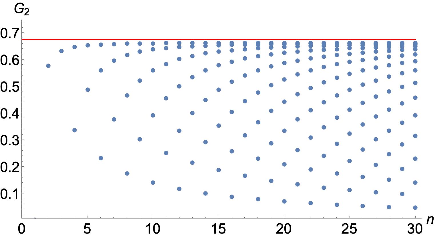
Figure 1: Positive zeros of $P_{n}(x)$ in (3) plotted as a function of $n$ up to $n=30$. The zeros are nondegenerate and range from 0 up to just below the exact value of $G_{2}=0.675978...$ (1) (heavy horizontal line).

Inaccuracy of DS approximants: The accuracy of the largest root in Fig. 7 improves slowly and monotonically with the order of the truncation. However, while the sequence of largest roots in Fig. 7 converges as $n\to\infty$, the limiting value is $0.663488...$, which is $1.85\%$ below the exact value of $G_{2}$ in (1). This discrepancy arises because truncating the DS equations means replacing $G_{2n}$ by $0$, but $G_{2n}$ is not small. The DS equations are exact, so we can compute $G_{2n}$ by substituting $G_{2}$ in (1) into (Underdetermined Dyson-Schwinger equations). We find that the Green’s functions grow rapidly with n: $G_{20}=-4.2788\times 10^{9}$, $G_{22}=3.0137\times 10^{11}$. Richardson extrapolation r6 yields the asymptotic behavior of $G_{2n}$:

$$G_{2n}\sim 2r^{2n}(-1)^{n+1}(2n-1)!\leavevmode\nobreak\ \leavevmode\nobreak\ (n\to\infty),$$ (4)

where $r=0.409\,505\,7...\,.$

Because the DS equations are algebraic when $D=0$, we can derive this asymptotic behavior analytically: We substitute $G_{2n}=(-1)^{n+1}(2n-1)!\,g_{2n}$, multiply the $2n$th DS equation by $x^{2n}$, sum from $n=1$ to $\infty$, and define the generating function $u(x)\equiv xg_{2}+x^{3}g_{4}+x^{5}g_{6}+...\,$. The differential equation satisfied by $u(x)$ is nonlinear:

$$u^{\prime\prime}(x)=3u^{\prime}(x)u(x)-u^{3}(x)-x,$$ (5)

where $u(0)=0$ and $u^{\prime}(0)=G_{2}$. We linearize (5) by substituting $u(x)=-y^{\prime}(x)/y(x)$ and get $y^{\prime\prime\prime}(x)=xy(x)$, where $y(0)=1$, $y^{\prime}(0)=0$, $y^{\prime\prime}(0)=-G_{2}$. The exact solution satisfying these initial conditions is

$$y(x)=\textstyle{\frac{2\sqrt{2}}{\Gamma(1/4)}\int_{0}^{\infty}}dt\,\cos(xt)\,e^{-t^{4}/4}.$$ (6)

If $y(x)=0$, the generating function $u(x)$ becomes infinite, so the smallest value of $|x|$ at which $y(x)=0$ is the radius of convergence of the series for $u(x)$. A simple plot shows that $y(x)$ vanishes at $x_{0}=\pm 2.441\,968\,2...$r7 . Therefore, $r=1/x_{0}=0.409\,506...\,$, which confirms (15).

The asymptotic behavior in (15) indicates that $G_{2n}$ grows much faster than the $\gamma_{2n}$ as $n\to\infty$:

$$\gamma_{2n}=\textstyle{\frac{\int_{-\infty}^{\infty}dx\,x^{2n}e^{-x^{4}/4}}{\int_{-\infty}^{\infty}dx\,e^{-x^{4}/4}}\sim 2^{n}\frac{\Gamma(n/2+1/4)}{\Gamma(1/4)}}.$$

This is astonishing because we get the connected Green’s functions by subtracting the disconnected parts from $\gamma_{2n}$.

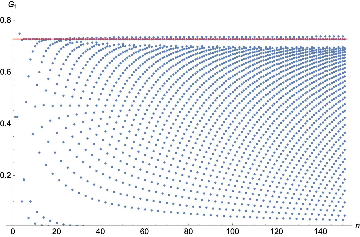
Figure 9: Absolute values of the solution to the truncated DS equations (12) assuming an asymptotic form for $G_{n}$, as given in Eq. (13) of the main text for $n$ up to 150. Rapid convergence to the exact value of $|G_{1}|=0.72901113\dots$, indicated by the heavy line, is observed.

Surprisingly, neglecting the huge quantity $G_{2n}$ on the left side of the DS equations (Underdetermined Dyson-Schwinger equations) still leads to a reasonably accurate result for $G_{2}$, as Fig. 7 shows. This is because while the term on the left side is big, the terms on the right are comparably big r7 . We also find that Padé approximants or mean-field-like schemes do not improve the convergence. But there is a way to get accurate results: Approximating the left side of the DS equations with the asymptotic formula in (15) gives $G_{2}$ to high precision (see Fig. 9. This approach works well for $D=0$ but is difficult to implement if $D>0$ as the DS equations are coupled nonlinear integral equations instead of algebraic equations.

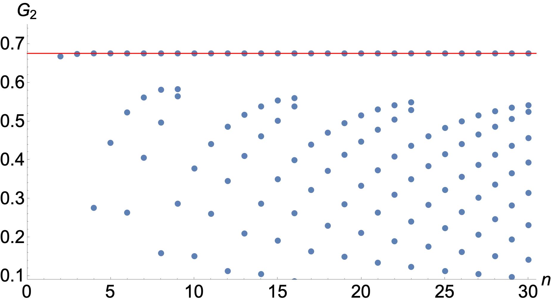
Figure 2: Dramatic improvement of the results in Fig. 7 obtained by replacing the left side of the DS equations (Underdetermined Dyson-Schwinger equations) by the asymptotic approximation (15) instead of zero.

Non-Hermitian cubic $D=0$ theory: The massless Lagrangian $\mathcal{L}=\mbox{$\textstyle{\frac{1}{3}}$}i\phi^{3}$ defines a non-Hermitian $\mathcal{PT}$-symmetric theory whose one-point Green’s function is

$$G_{1}=\textstyle{\int}dx\,xe^{-ix^{3}/3}\big{/}\textstyle{\int}dx\,e^{-ix^{3}/3},$$ (7)

where the path of integration terminates in a $\mathcal{PT}$-symmetric pair of Stokes sectors r5 , so the exact value of $G_{1}$ is $G_{1}=-i3^{1/3}\Gamma\big{(}\mbox{$\textstyle{\frac{2}{3}}$}\big{)}\big{/}\Gamma\big{(}\mbox{$\textstyle{\frac{1}{3}}$}\big{)}=-0.729\,011\,13...\,i.$

The first four DS equations are

$$\!\!\!\!\!\!\!\!G_{2}=-G_{1}^{2},\leavevmode\nobreak\ G_{3}=-2G_{1}G_{2}-i,$$

$$\!\!\!\!\!\!\!\!G_{4}=-2G_{2}^{2}-2G_{1}G_{3},\leavevmode\nobreak\ G_{5}=-6G_{2}G_{3}-2G_{1}G_{4}.$$ (8)

To obtain the leading approximation to $G_{1}$ we substitute the first equation into the second and truncate by setting $G_{3}=0$. The resulting equation is $G_{1}^{3}=\mbox{$\textstyle{\frac{1}{2}}$}i$ and the solution that is consistent with $\mathcal{PT}$ symmetry is $G_{1}=-2^{-1/3}i=-0.793\,700\,53...\,i$. This result differs by $8.9\%$ from the exact value of $G_{1}$.

At higher order we again truncate the system and find the roots of the associated polynomial in $G_{1}$. At first, the roots consistent with $\mathcal{PT}$ symmetry obtained by this procedure approach the exact $G_{1}$ but unlike the roots for the Hermitian quartic theory, where the approach is monotone (Fig. 7), the approach is oscillatory: For the $n=4,5,6,7$ truncations the closest roots to the exact $G_{1}$ are $-0.693\,361...\,i$, $-0.746\,900...\,i$, $-0.712\,564...\,i$, and $-0.739\,871...\,i$. However, for $n=8$ this pattern breaks; the closest root is $-0.712\,368...\,i$, which is a worse approximation than the $n=6$ root.

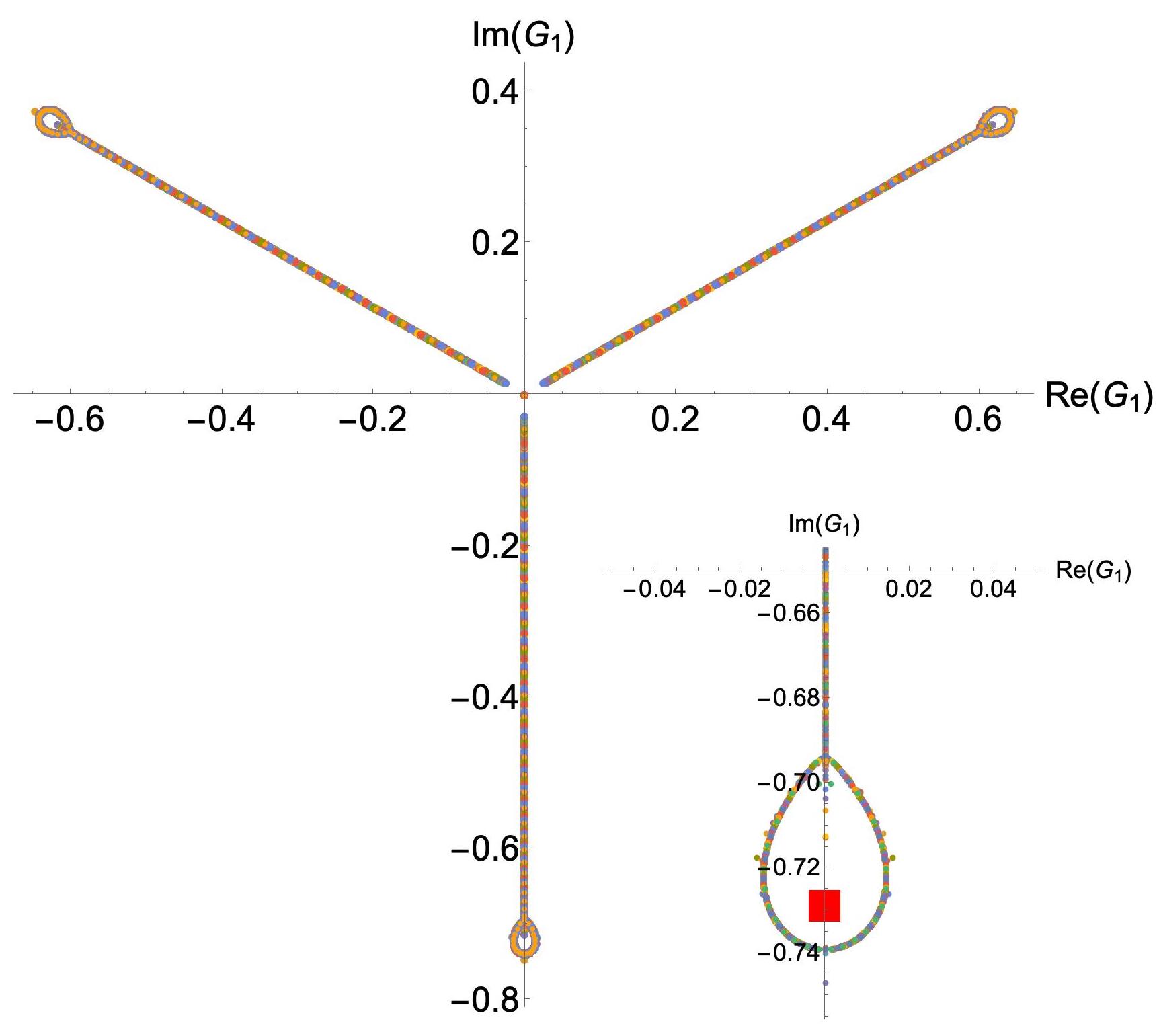
Figure 3: All solutions of the truncated DS equations (8) for the non-Hermitian cubic theory. Inset: The square indicates the exact $G_{1}=-0.729\,011\,13...\,i$.

This departure from oscillatory convergence is the first indication of a qualitative change in the approximants. For $n=10$ the roots closest to $G_{1}$ are a pair on either side of the negative-imaginary axis at $-0.717\,367...\,i\pm 0.016\,050...\,$. We solve the DS equations up to the 150th truncation and plot in Fig. 3 all roots from $n=2$ to 150 as dots in the complex plane. These roots become dense on a three-bladed propeller shape, with a small loop at the tip of each blade. The inset shows that dots on the loop surround but do not approach the exact $G_{1}$.

The roots in Fig. 3 have threefold symmetry because the truncated DS equations give polynomials having only powers of $x^{3}$ (apart from a root at 0). The DS equations depend only locally on the integrand of the functional integral; they are totally insensitive to the boundary conditions on the functional integrals. There are three pairs of Stokes sectors of angular opening $60^{\circ}$ inside of which the integration path in (7) can terminate. These sectors are centered about $\theta_{1}=\frac{\pi}{2}$, $\theta_{2}=-\frac{\pi}{6}$, or $\theta_{3}=-\frac{5\pi}{6}$. If the integration path terminates in the $\mathcal{PT}$-symmetric (2,3) sectors, $G_{1}$ is negative imaginary, but if it terminates in the (1,2) or (1,3) sectors, $G_{1}$ is complex.

Asymptotic behavior of $G_{n}$ for large $n$: Richardson extrapolation gives the large-$n$ behavior of the exact Green’s functions for the cubic theory ($G_{14}=42\,692.806\,116$, $G_{15}=-255\,589.034\,701\,i$):

$$G_{n}\sim-(n-1)!\,r^{n}(-i)^{n}\quad(n\to\infty),$$ (9)

where $r=0.427\,696\,347\,707...\,$. Equation (9) is analogous to (15) for the Hermitian quartic theory, and can be confirmed analytically r7 .

To calculate $r$ analytically we follow the procedure used above for the Hermitian quartic theory. Define $g_{p}\equiv-i^{n}G_{p}/(p-1)!$ and rewrite the DS equations for the Green’s functions $G_{n}$ as one compact equation:

$$g_{p}=\textstyle{\frac{1}{p-1}\sum_{k=1}^{p-1}g_{k}g_{p-k}+\frac{1}{2}\delta_{p,3}}\quad(p\geq 2).$$

Next, multiply by $(p-1)x^{p}$, sum from $p=2$ to $\infty$, and define the generating function $f(x)\equiv\sum_{p=1}^{\infty}x^{p}g_{p}$, which obeys the Riccati equation $xf^{\prime}(x)-f(x)=f^{2}(x)+x^{3}$.

Substituting $f(x)=-xu^{\prime}(x)/u(x)$ linearizes this equation: $u^{\prime\prime}(x)=-xu(x)$. This is an Airy equation whose general solution is $u(x)=a\,{\rm Ai}(-x)+b\,{\rm Bi}(-x)$. From $f^{\prime}(0)=g_{1}=-3^{1/3}\Gamma\big{(}\mbox{$\textstyle{\frac{2}{3}}$}\big{)}/\Gamma\big{(}\mbox{$\textstyle{\frac{1}{3}}$}\big{)}$ we find that $a$ is arbitrary and $b=0$, so $f(x)=x\,{\rm Ai}^{\prime}(-x)/{\rm Ai}(-x)$.

The power series for the generating function $f(x)$ blows up when the denominator vanishes, when $x=2.338\,107\,410\,460\,...$. This is the radius of convergence of the series and its inverse is the value of $r$ in (9).

The rapid growth of $G_{n}$ in (9) explains the slow convergence and inaccurate numerical results obtained by truncating the DS equations (Fig. 3). Once again, using this asymptotic approximation instead of setting $G_{n}=0$ gives extremely accurate and rapidly convergent approximations to $G_{1}$ r7 .

Non-Hermitian quartic $D=0$ theory: The Lagrangian $\mathcal{L}=-\mbox{$\textstyle{\frac{1}{4}}$}\phi^{4}$ defines a non-Hermitian $\mathcal{PT}$-symmetric theory where

$$G_{1}=\textstyle{\frac{\int dx\,x\exp\big{(}x^{4}/4\big{)}}{\int dx\,\exp\big{(}x^{4}/4\big{)}}=-\frac{2i\sqrt{\pi}}{\Gamma(1/4)}}=-0.977\,741...\,i,$$

and the path of integration lies inside a $\mathcal{PT}$-symmetric pair of Stokes sectors in the lower-half complex-$x$ plane.

The first three DS equations are

$$G_{3}=-G_{1}^{3}-3G_{1}G_{2},$$

$$G_{4}=-3G_{1}G_{3}-3G_{2}^{2}-3G_{1}^{2}G_{2}-1,$$

$$G_{5}=-3G_{1}G_{4}-9G_{2}G_{3}-3G_{1}^{2}G_{3}-6G_{1}G_{2}^{2}.$$ (10)

Solving these equations is harder than for the Hermitian quartic or the non-Hermitian cubic theory, as two Green’s functions must be set to zero to close the system, and two coupled polynomials equations must be solved simultaneously. The leading-order truncation leads to: $G_{1}=-i\,(3/2)^{1/4}=-1.106682...\,i$, which differs from the exact $G_{1}$ above by $13.2\%$.

This procedure is continued for larger $n$. The number of roots increases rapidly and the roots have fourfold symmetry in the complex plane. All roots up to $n=33$ are shown in Fig. 4. There are four concentrations of roots on the axes but $\mathcal{PT}$ symmetry requires that $G_{1}$ be negative imaginary. Unlike Fig. 3 the dots are scattered over the complex plane because truncating the DS equations gives two coupled polynomial equations.

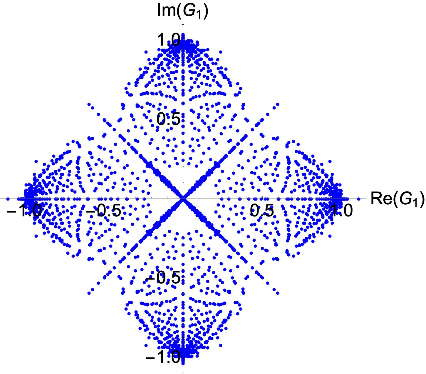
Figure 4: All roots $G_{1}$ up to $n=33$ plotted as points in the complex plane. The roots exhibit fourfold symmetry but only those on the negative-imaginary axis respect $\mathcal{PT}$ symmetry.

We can determine the asymptotic behavior of $G_{n}$ for large $n$ from the DS equations in (10). We find $G_{n}\sim-i(n-1)!\,(-i)^{n}r^{n}$, where $r=0.34640...\,$. This result is analogous to the asymptotic behavior in (9).

Quintic and sextic $D=0$ theories: The DS equations for the $\mathcal{PT}$-symmetric $D=0$ Lagrangian $-\mbox{$\textstyle{\frac{1}{5}}$}i\phi^{5}$ require that three higher Green’s functions be set to 0 to close the truncated system, leading to three coupled polynomial equations for $G_{1}$, $G_{2}$, and $G_{3}$. Going to the $n=11$ truncation we see ten concentrations of roots in Fig. 5. (The DS equations are insensitive to the choice of Stokes sectors for the functional integral.) There are two pairs of $\mathcal{PT}$-symmetric boundary conditions, which give rise to two imaginary values of $G_{1}=0.412\,009...\,i$ and $G_{1}=-1.078\,653...\,i$r8 , seen on Fig. 5 as heavy dots.

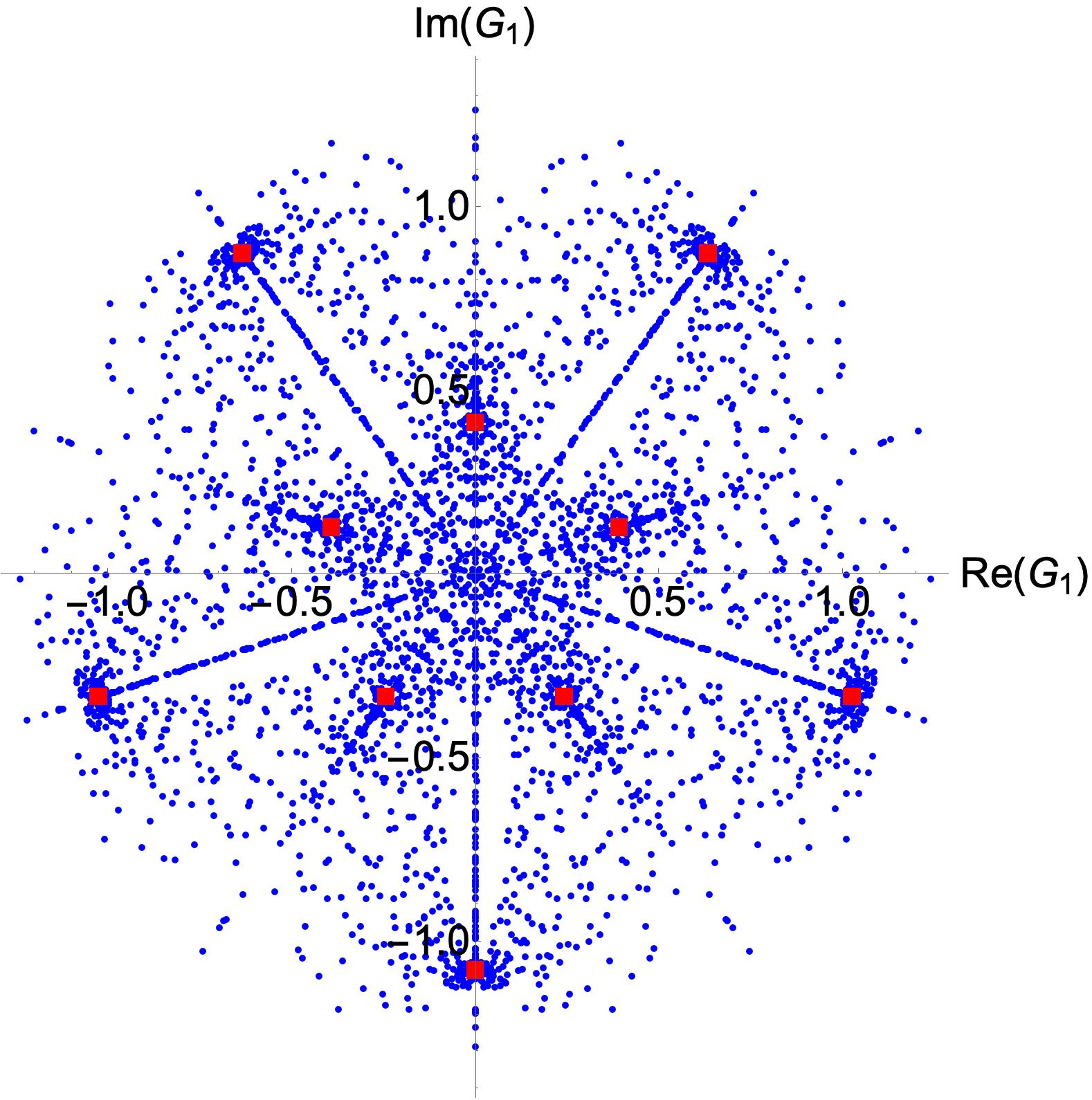
Figure 5: Solutions to the DS equations for a quintic $D=0$ field theory. Exact values are denoted by squares.

For the sextic case $\mathcal{L}=\mbox{$\textstyle{\frac{1}{6}}$}\phi^{6}$ we truncate the DS equations and set the four highest Green’s functions to 0. We must solve four coupled polynomial equations. To reduce the number of solutions we impose parity symmetry, so $G_{1}=G_{3}=0$. This eliminates all but three pairs of Stokes sectors. Figure 6 shows three concentrations of roots for $G_{2}$ up to the $n=32$ truncation. The exact values of $G_{2}$ (squares) are $6^{1/3}\sqrt{\pi}/\Gamma(1/6)=0.578\,617...$ and $-0.289\,302...\pm 0.501\,097\,i$; the error is a few percent.

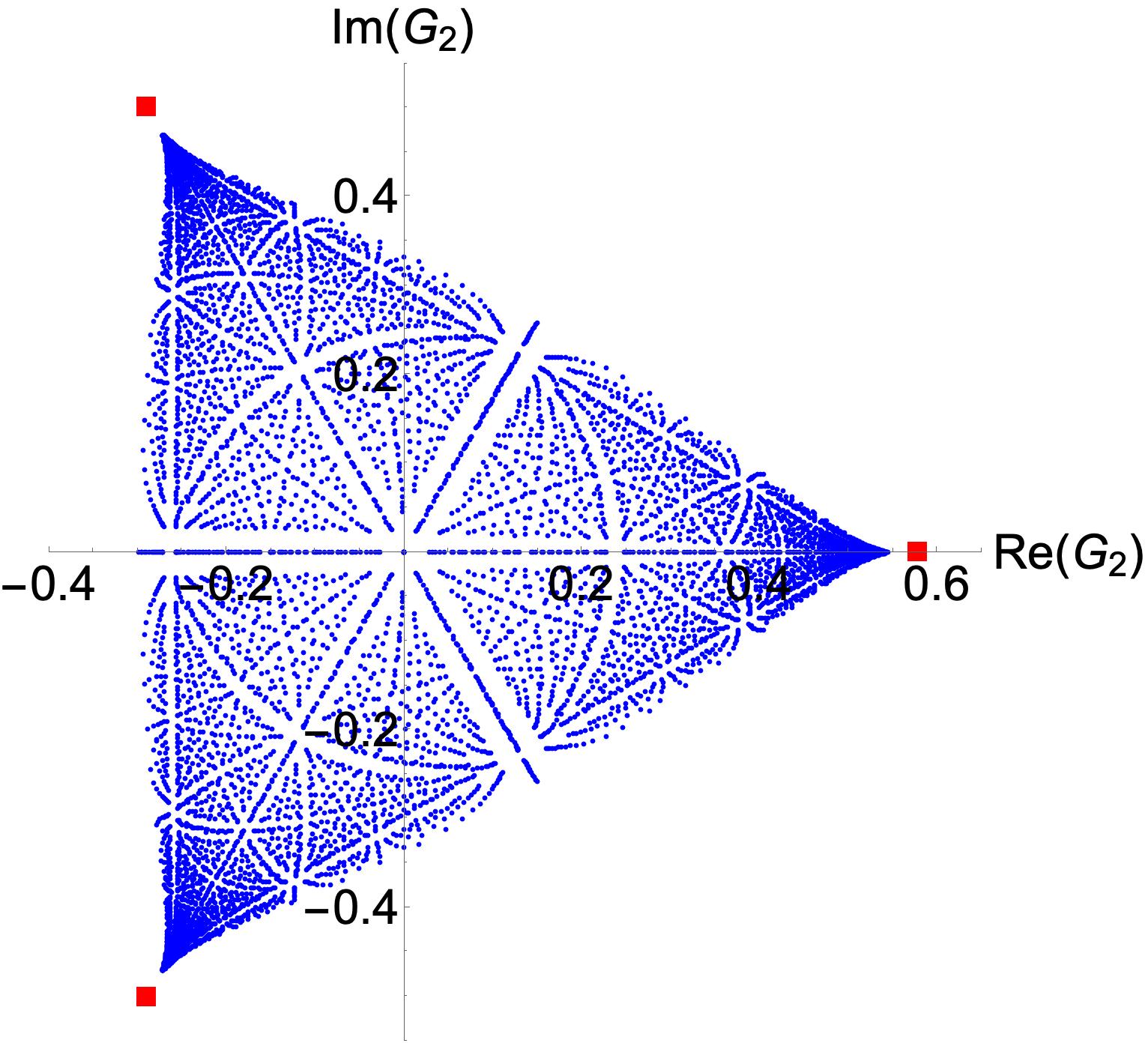
Figure 6: Sextic case showing three concentrations of parity-symmetric solutions for $G_{2}$ differing from the exact values (squares) by a few percent.

Summary: For five $D=0$ field theories we have shown that the truncated DS equations yield underdetermined polynomial systems. There is no effective strategy to solve such systems: Closing the systems by setting higher Green’s functions to zero gives sequences of approximants that converge to incorrect limiting values. Replacing higher Green’s functions with mean-field-like approximations also gives incorrect limiting values, and this approach has the drawback that if $D>0$, renormalization is required. The one numerically accurate approach is to replace the higher $G_{n}$’s by their large-$n$ asymptotic behaviors. This is difficult when $D>0$, but we believe that it may be possible to calculate, and it presents an interesting avenue for further research.

This study emphasizes that the DS equations are local. Deriving the DS equations assumes only that the functional integrals exist; the DS equations are insensitive to which Stokes sectors in function space are used. As a result, the approximants try (but fail) to approach many different limits, most of which are complex r9 .

The accuracy of the DS truncations worsens when interaction terms have higher powers of the field because the indeterminacy of the system increases. More Green’s functions must be set to 0 to close the truncated system.

For Lagrangians having a weak-coupling constant $g$ we can expand all $G_{n}$ in the DS equations as series in powers of $g$. This removes all ambiguities discussed in here and gives the unique weak-coupling expansion for each $G_{n}$. However, this merely replicates a Feynman-diagram calculation of the Green’s functions and totally ignores the nonperturbative content of the theory.

Supplemental Material to "Underdetermined Dyson-Schwinger equations"

I Derivation of the DS equations for $D=1$

The DS equations follow directly on differentiating the functional integral for $Z[J]$ (or $\log(Z[J])$) with respect to $J$, giving $\gamma_{n}$ (or $G_{n}$),

$$Z[J]=\textstyle{\int\mathcal{D}\phi\,\exp\int dx}\{-\mathcal{L}[\phi(x)]+J(x)\phi(x)\}.$$

($\mathcal{L}$ is the Lagrangian, $J$ is a c-number source, and $Z[0]$ is the Euclidean partition function.)

For example, for a $D=1$ Hermitian quartic theory,

$$Z[J]={\textstyle\int}D\phi\,\exp\big{[}\textstyle{\int}dt(-\mbox{$\textstyle{\frac{1}{2}}$}{\dot{\phi}}^{2}-\mbox{$\textstyle{\frac{1}{4}}$}\phi^{4}+J\phi)\big{]}.$$ (11)

We take the VEV of the field equation $-{\ddot{\phi}}(t)+\phi^{3}(t)-J(t)=0$ and divide by $Z[J]$:

$$-{\ddot{G}}_{1}(t)+\gamma_{3}(t,t,t)/Z[J]=J(t).$$ (12)

Note that $G_{1}(t)$ and $\gamma_{3}(t,t,t)$ are functionals of $J$.

We calculate $\gamma_{3}$ by differentiating $\gamma_{1}(t)=\langle 0|\phi(t)|0\rangle=Z[J]G_{1}(t)$ twice with respect to $J(t)$:

$$\gamma_{2}(t,t) = \langle 0|\phi^{2}(t)|0\rangle=Z[J]G_{2}(t,t)+Z[J]G_{1}^{2}(t),$$

$$\gamma_{3}(t,t,t) = \langle 0|\phi^{3}(t)|0\rangle=Z[J]G_{3}(t,t,t)$$

$$\!\!\!+3Z[J]G_{1}(t)G_{2}(t,t)+Z[J]G_{1}^{3}(t).$$

We then divide by $Z[J]$ and eliminate $\gamma_{3}$ in (12):

$$-{\ddot{G}}_{1}(t)+G_{3}(t,t,t)+3G_{1}(t)G_{2}(t,t)+G_{1}^{3}(t)=J(t).$$ (13)

We obtain the DS equations from (13) by repeated functional differentiation with respect to $J$. For the first DS equation we set $J\equiv 0$. Parity invariance implies that odd-numbered Green’s functions vanish, so the first DS equation is trivial: $0=0$. For the second DS equation we differentiate (13) with respect to $J(s)$ and set $J\equiv 0$:

$$-{\ddot{G}}_{2}(s-t)+M^{2}G_{2}(s-t)+G_{4}(s,t,t,t)=\delta(s-t),$$ (14)

where the renormalized mass is $M^{2}=3G_{2}(0)$.

Equation (14) is one equation in two unknowns, $G_{2}$ and $G_{4}$. (Each new DS equation introduces one new unknown.) To proceed, we simply set $G_{4}=0$ in (14) and Fourier transform to get $(p^{2}+M^{2}){\tilde{G}}_{2}(p)=1$. The inverse transform gives $G_{2}(t)=e^{-M|t|}/(2M)$, so $G_{2}(0)=1/(2M)$, yielding the solution is $M=(3/2)^{1/3}=1.145...\,$. This renormalized mass is the first excitation above the ground state and for this model $M=E_{1}-E_{0}=1.088...\,$. Thus, the leading-order DS result is 5.2% high.

Next, we examine a $\mathcal{PT}$-symmetric quartic theory in $D=1$; we change the sign of the $\phi^{4}$ term in (11) r5 . The Green’s functions are not parity symmetric, so the odd-$n$ $G_{n}$’s do not vanish. The first DS equation is nontrivial: $3G_{1}G_{2}(0)+G_{1}^{3}=0$. The second DS equation leads to two equations: $M^{2}=-3[G_{1}^{2}+G_{2}(0)]$ and $G_{2}(0)=1/(2M)$. We solve these three equations: $M=3^{1/3}=1.442...\,$. The exact value of $M$ obtained by solving the Schrödinger equation for the $\mathcal{PT}$-symmetric quantum-mechanical Hamiltonian $H=\mbox{$\textstyle{\frac{1}{2}}$}p^{2}-\mbox{$\textstyle{\frac{1}{4}}$}x^{4}$ is $E_{1}-E_{0}=1.796...$, so the DS result is 19.7% low.

These two examples motivate us to ask if higher truncations improve the accuracy, but this leads to nonlinear integral equations requiring detailed numerical analysis. However, we can solve the DS equations in high order when $D=0$, which we do for five $D=0$ field theories.

II Hermitian quartic theory in D=0

As observed in the main text, Eq. (8), the asymptotic behavior of the Green’s functions for the Hermitian quartic theory was determined to be

$$G_{2n}\sim 2r^{2n}(-1)^{n+1}(2n-1)!\leavevmode\nobreak\ \leavevmode\nobreak\ (n\to\infty),$$ (15)

where $r=0.409\,505\,7...\,.$. Clearly $G_{2n}$ grows rapidly with $n$, so that it is surprising that the procedure of truncation still leads to a relatively accurate result, as was shown in Fig. 1 of the main text. We have argued that this is because, while the exact value of the left hand side of the appropriate equation in Eq. (6) is big, the terms on the right hand side are comparably big.

The numerical technique of Legendre interpolation provides a useful analogy r1 . Given $n$ data points $x_{1},\,...,\,x_{n}$ at which we measure a function $f(x)$, $f(x_{1})=f_{1},\leavevmode\nobreak\ ...,\leavevmode\nobreak\ f(x_{n})=f_{n}$, one can fit this data with a polynomial $P_{n-1}(x)$ of degree $n-1$ that passes exactly through the value $f(x_{k})$ at $x=x_{k}$ for $1\leq k\leq n$. There is a simple formula for this polynomial. The problem with this construction is that between data points the polynomial exhibits huge oscillations where it becomes alternately large and positive and large and negative due to a fundamental instability associated with high-degree polynomials. To avoid this instability, which is associated with the stiffness of polynomials, one can use a least-squares fit, which passes near but not exactly through the input data points. This is why cubic splines are used to approximate functions rather than, say, octic splines. The instability associated with high-degree polynomials allows the DS approach to work fairly well. If we use the exact values of the Green’s functions on the right side, we obtain the exact value of the Green’s function on the left side, which is a huge number. Evidently, changing the Green’s functions on the right side of Eq. (6) of the main text slightly by replacing the exact values by approximate values of the lower Green’s functions now gives 0, instead of $G_{2n}$.

To determine the asymptotic behavior of $G_{2n}$ analytically, we defined a generating function, which, after manipulation, leads to the expression for $y(x)$ given in Eq. (10) of the main text,

$$y(x)=\textstyle{\frac{2\sqrt{2}}{\Gamma(1/4)}\int_{0}^{\infty}}dt\,\cos(xt)\,e^{-t^{4}/4}.$$

We plot $y(x)$ in Fig. 7, from which one can determine the zero nearest to the origin. This lies at $x_{0}=\pm 2.4419682...$, and has the inverse 0.409506…, corresponding to the value of $r$ found numerically through Richardson extrapolation.

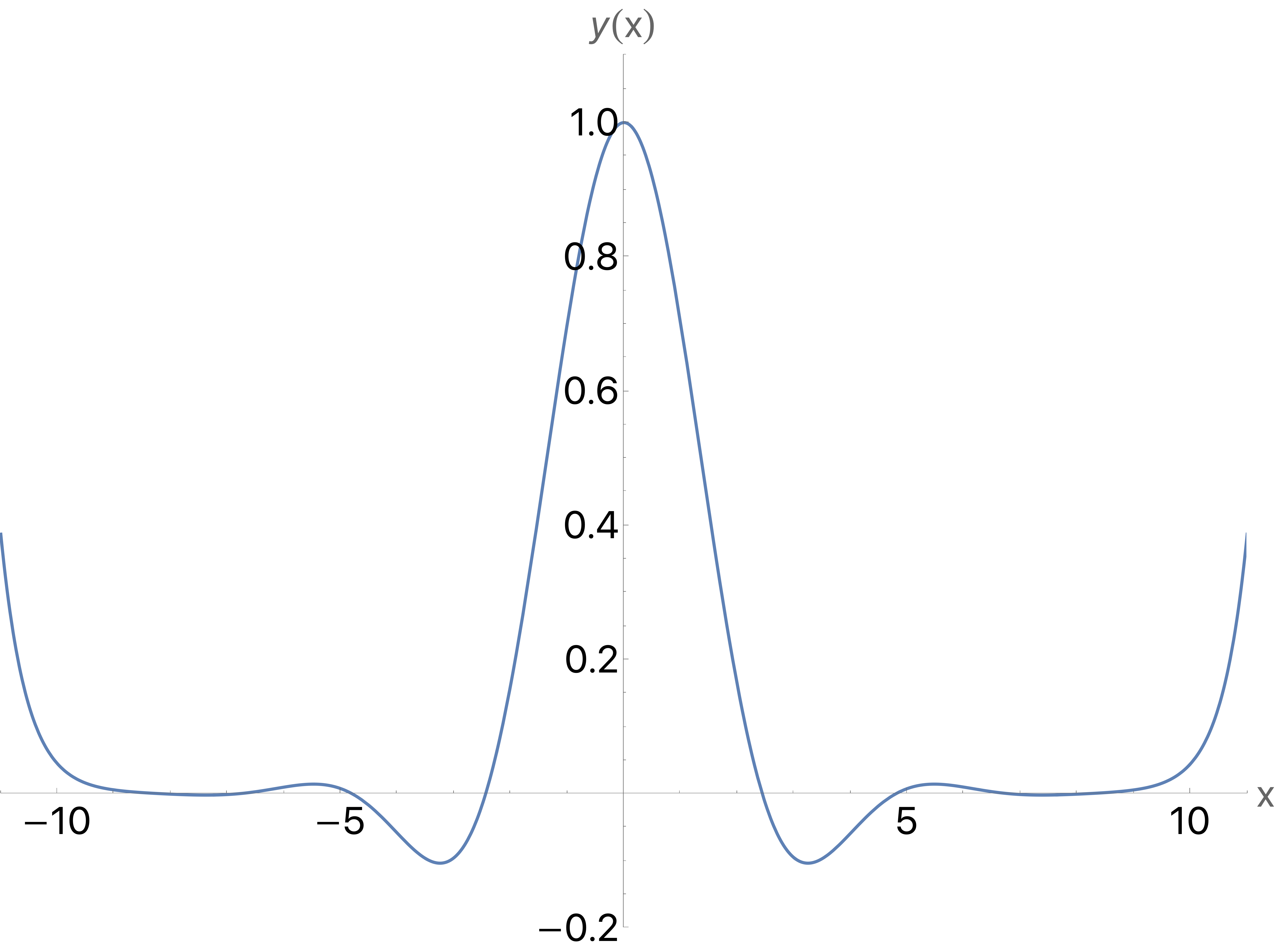
Figure 7: Plot of $y(x)$ normalized to $y(0)=1$. The function $y(x)$ is even. The zero nearest to the origin lies at $x_{0}=\pm 2.4419682...$ the inverse of this number is 0.409506…, which confirms the numerical result for $r$ below Eq. (8) of the main text.

III non-Hermitian cubic theory in $D=0$

We first comment that the roots in Fig. 2 of the main paper have threefold symmetry because the truncated DS equations give polynomials having only powers of $x^{3}$ (apart from a root at 0). The DS equations depend only locally on the integrand of the functional integral; they are totally insensitive to the boundary conditions on the functional integrals. There are three pairs of Stokes sectors of angular opening $60^{\circ}$ inside of which the integration path can terminate. These sectors are centered about $\theta_{1}=\frac{\pi}{2}$, $\theta_{2}=-\frac{\pi}{6}$, or $\theta_{3}=-\frac{5\pi}{6}$. If the integration path terminates in the $\mathcal{PT}$-symmetric (2,3) sectors, $G_{1}$ is negative imaginary, but if it terminates in the (1,2) or (1,3) sectors, $G_{1}$ is complex.

Secondly, using the asymptotic approximation to $G_{n}$ given in Eq. (13) of the main text to calculate the successive orders of approximation to $G_{1}$ leads to extremely accurate and rapidly convergent values of $G_{1}$. As we are only interested in solutions along the negative imaginary axis, in Fig. 8 we show a sector of the complex plane calculated in this way, together with the standard truncation scheme $G_{n}=0$. This can be compared with the inset in Fig. 3 of the main text. Using the asymptotic expansion evidently leads to many solutions in the complex plane. In addition, an accurate value of $G_{1}$ appears on the imaginary axis. This can be best seen by plotting the absolute values of $G_{1}$ as a function of $n$, and which is presented in Fig. 3. In addition to the solution lying numerically above the absolute value of $G_{1}$, the exact solution also emerges.

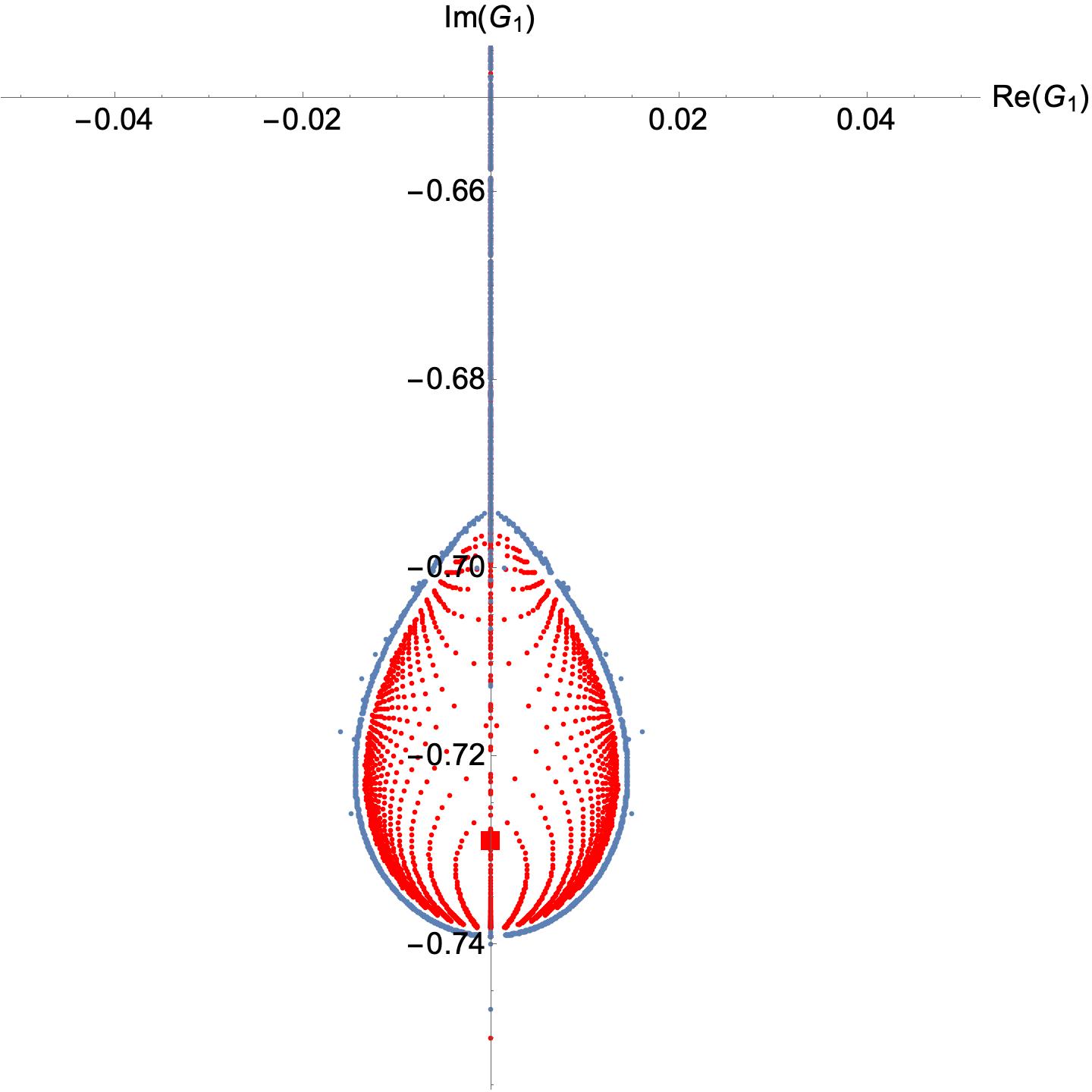
Figure 8: Solutions of the truncated DS equations (12) of the main text, for the non-Hermitian cubic theory, corresponding to Fig. 3 of the main text. In addition to the solution shown there, we include solutions based on the asymptotic behavior of $G_{n}$ (internal structure in the loop). This leads to a distribution pattern in the complex plane, as well as a rapid convergence to the exact value of $G_{1}=-0.72901113\dots i$, which is indicated by the square.

References

- (1) C. M. Bender et al., PT Symmetry: in Quantum and Classical Physics (World Scientific, Singapore, 2019).
- (2) H. P. Greenspan and D. J. Benney, Calculus: An Introduction to Applied Mathematics (McGraw-Hill, New York, 1973)
- (3) C. M. Bender and S. P. Klevansky, Phys. Rev. Lett. 105, 031601 (2010).