Comparison of Motion Encoding Frameworks on
Human Manipulation Actions

Abstract

Movement generation, and especially generalisation to unseen situations, plays an important role in robotics. Different types of movement generation methods exist such as spline based methods, dynamical system based methods, and methods based on Gaussian mixture models (GMMs). Using a large, new dataset on human manipulations, in this paper we provide a highly detailed comparison of three most widely used movement encoding and generation frameworks: dynamic movement primitives (DMPs), time based Gaussian mixture regression (tbGMR) and stable estimator of dynamical systems (SEDS). We compare these frameworks with respect to their movement encoding efficiency, reconstruction accuracy, and movement generalisation capabilities. The new dataset consists of nine object manipulation actions performed by 12 humans: pick and place, put on top/take down, put inside/take out, hide/uncover, and push/pull with a total of 7,652 movement examples. Our analysis shows that for movement encoding and reconstruction DMPs are the most efficient framework with respect to the number of parameters and reconstruction accuracy if a sufficient number of kernels is used. In case of movement generalisation to new start- and end-point situations, DMPs and task parameterized GMM (TP-GMM, movement generalisation framework based on tbGMR) lead to similar performance and outperform SEDS. Furthermore we observe that TP-GMM and SEDS suffer from inaccurate convergence to the end-point as compared to DMPs. These different quantitative results will help designing trajectory representations in an improved task-dependent way in future robotic applications.

I Introduction

Movement generation methods play an important role in robotics that is crucial for enabling robots to perform actions precisely, and especially to generalise movements to unknown situations. Apart from industrial applications, where fast and reliably repetitive movements are needed, static, non-adaptive trajectory representations such as interpolation between via-points using splines [1] are insufficient in most cases. In dynamic environments, trajectories need to be adapted, and it is infeasible to pre-program trajectories for each possible situation. Therefore, motion encoding frameworks need to be able to generalize movements to new situations, e.g., to new start- or end-points. Furthermore, this way they are more easily allowing for learning by demonstration [2, 3], also called transfer learning or imitation learning. In imitation learning, instead of obtaining new movements by a theoretical description or optimization method, human demonstrations are encoded by some mathematical model and then used by a robot. Human demonstrations are usually obtained by manually moving the robot, called kinesthetic guidance, or via motion tracking of the human body.

To generalize trajectories to new situations, a motion encoding framework should therefore be able to generate human like movements for new situations from given demonstrations of known situations. As will be discussed below, various different approaches were developed for movement generalization, however the question arises, which of these frameworks performs best with respect to efficiency and accuracy of movement encoding and generalization to unseen situations.

Dynamical Movement Primitives (DMPs, [4]) are one of the most frequently used encoding frameworks. There, a critically damped linear attractor system is forced to follow a desired trajectory by a nonlinear term that is approximated by a weighted sum of Gaussian kernels. There exist several related frameworks which also operate on dynamical systems, for example Via-Point Movement Primitives [5] that increase the capability of the system to adapt to new situations using via-points along the trajectory. A different approach that also uses a representation as a dynamical system are Optimal Control Primitives [6]. There, the trajectories are represented with Chebyshev polynomials instead of Gaussian kernels. A linear-quadratic regulator, derived from optimal control theory (hence the name), ensures the accurate reproduction of the trajectories and robustness against perturbations. All these frameworks are based on the common ground of dynamical systems with implicit time dependence, which means that the trajectories are obtained by integrating a specially designed dynamical system that then generates the desired trajectories.

Another class of approaches uses Gaussian Mixture Models (GMMs) to encode trajectories. Since GMMs in general are a model for regression of arbitrary distributions, they are commonly used for many other applications in statistics and data science. Moreover, they can also be used to estimate the parameters of frameworks with dynamical systems similar to the methods above [7, 8]. One key difference to the previously mentioned methods is that GMMs are able to encode multidimensional trajectories in one model, and thus, encode correlations between the dimensions, while most dynamical systems-based approaches use as many independent 1D systems as there are dimensions in the trajectory. GMM based models can also work completely without dynamical systems, for example by encoding the joint distribution of position and time and extracting the trajectory using the conditional distribution of position given time [9]. Recently, a deep learning based approach was proposed to encode GMMs using a mixture density network (MDN, [10]).

Methods like Probabilistic Movement Primitives [11] exist, which can encode cross-correlations, too; but their working principle of modelling distributions over trajectories is closer to the GMM models than to DMPs.

There exist several papers comparing different models either only theoretically, e.g., for DMPs [12], or with application on a common task, e.g., for DMPs, PMPs and OCPs [6] or for different kinds of GMM encodings [13]. Those papers compare relatively similar frameworks on small datasets and their respective tasks are not comparable between each other. There also exists a study on benchmarking of different models [14] which focuses on measures to judge the human-likeness of actions generated by several different frameworks, as well as their robustness to perturbations. This benchmarking was performed on a dataset of handwriting trajectories, however, there was no quantitative comparison of generalized trajectories (i.e., with respect to the changed end-point) to ground truth (human) trajectories. In the current work we aim to provide a thorough analysis and comparison of different type models on a larger dataset (9 different action classes; 7,652 movement trajectories in total) with the focus on generalization of point-to-point human hand movements to new start-/end-positions that plays an important role for generation of human-like robotic manipulation actions in unknown situations.

We compare three different frameworks, namely DMPs [4], task parameterized GMMs (TP-GMMs) with time based Gaussian Mixture Regression (tbGMR, [9]) and trajectory encoding and generation using stable estimator of dynamical systems (SEDS, [8]). All these motion encoding frameworks have been widely used for robot motion control and demonstration learning [15, 16, 17, 2, 3]. We quantitatively analyze and compare the performance of the frameworks for movement encoding and reconstruction, and for generalization from demonstrations to new situations on a novel very large dataset of human manipulation actions. The main novel aspect compared to the previous work and the key focus of this study is on how well different movement generation frameworks are able to generalise to new situations in comparison to human movements.

First, we investigate how well the frameworks are able to encode and reconstruct single trajectories from the action dataset. Second, we also test generalization capabilities of the frameworks by presenting subsets of the dataset as training demonstrations and testing generalization capabilities on different situations obtained from remaining demonstrations. Here we evaluate how similar trajectories generated by different models are to the human movements. Furthermore, we also compare how many free parameters the models need to achieve their respective movement encoding and reconstruction, and generalization performance.

II Materials and Methods

II-A Movement Dataset

II-A1 Recording setup

To test the performance of the selected models on human manipulation actions we recorded a dataset of simple manipulation actions using a multi camera recording setup (see Figure 1(a)). Movements were recorded with five calibrated and synchronized cameras at 100 Hz with a resolution of $1024\times 768$ pixels. Movement trajectories were extracted as described in Section II-A3 below.

II-A2 Manipulation actions

We selected nine different manipulation actions from [18] all of which included only one object, which was actively manipulated. All actions are listed with a short description in Table I (see also supplementary video).

We used five different objects in the experiments as shown in Figure 1(c). A red wooden cube of dimensions 8 cm x 8 cm x 6 cm was used as the main manipulation object. It was open at the bottom and hollow inside, such that it could also be used to hide and uncover a smaller blue cube.

Most of the actions also included a second fixed object, called the “target object”. We used three bowl-like target objects of different height for the put on top/take down and put inside/take out actions. These objects were turned around to give raised bases of different height for the put on top and take down actions.

To control the start and end positions of the movements, we restricted them to a square grid with 10 cm grid spacing and chose the target positions to cover a range of different directions as shown by arrows in Figure 2. The movements in group 1 are frontal, in group 2 lateral, and groups 3 and 4 contain moves in mixed directions.

We obtained data from 12 adult participants, 4 females and 8 males. Each participant performed nine actions as detailed in Table I to the 13 different start-/end-points (see Figure 2). When using one of the bowl-like target objects, the moves to (3,0) and (4,1) were omitted due to space constraints, leaving only 11 start-/end-points. Each movement was repeated three times to accommodate for variability in the human demonstrations. Note that in some cases accidentally people performed two or four demonstrations instead of three. In total, our dataset consisted of 7,652 movements.

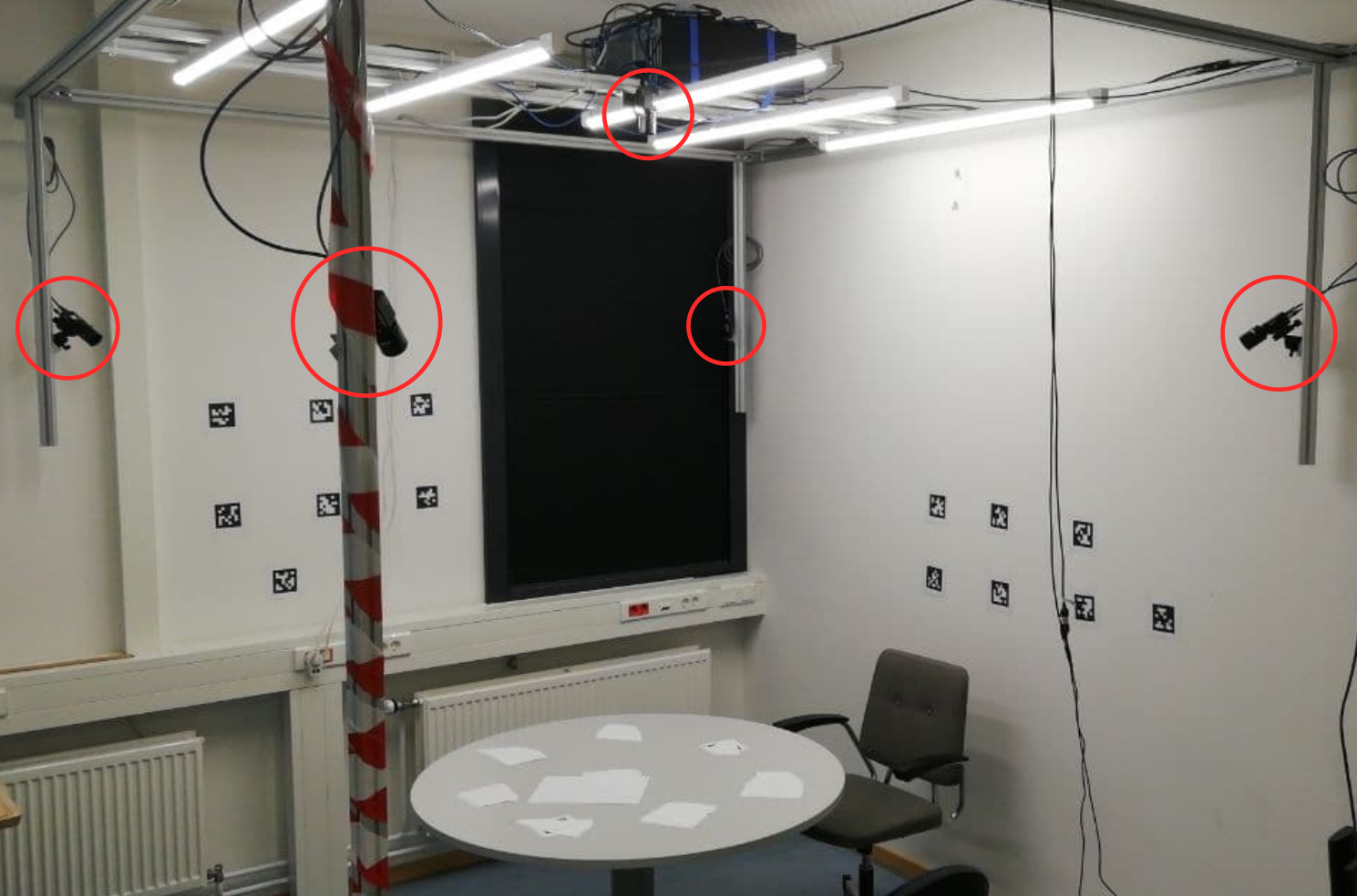
(a) The multi-camera recording setup with one top-view and four side-view cameras (marked by red circles).

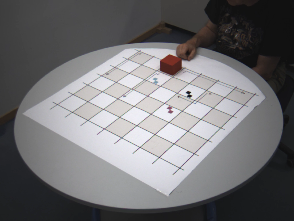
(b) Table setup view with the checkerboard mat.

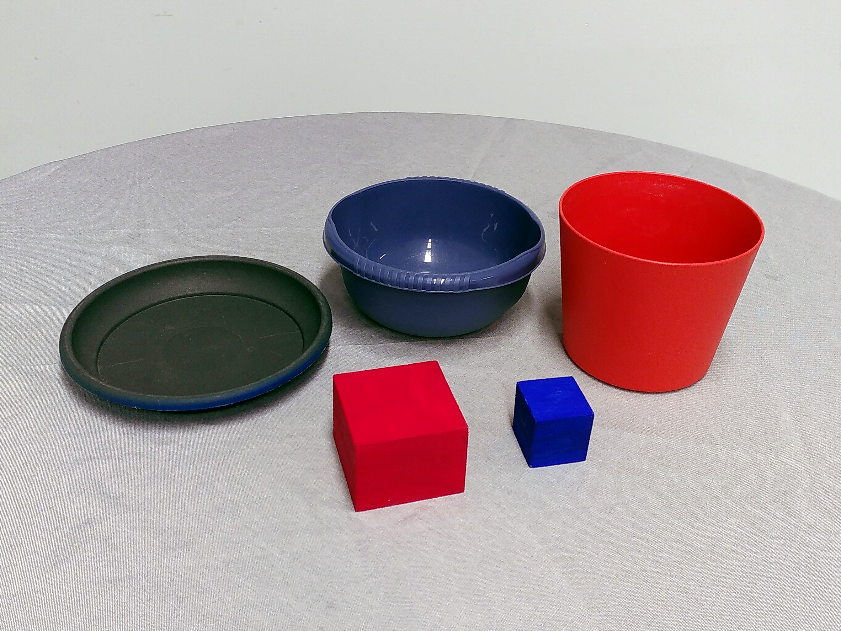
(c) Objects used for the recordings.

Figure 1: Recording setup.

TABLE I: List of the selected movements and short descriptions.

Movement	Description
pick and place	Pick up the manipulation object and place it at the target position.
put on top / take down	Put the manipulation object on top of the target object /
	take it down on the table at the start position.
put inside / take out	Put the manipulation object inside the bowl-like target object /
	take it out and place it on the table at the start position.
hide / uncover	Put the manipulation object over the smaller target object /
	take if off and place it on the table at the start position.
push / pull	Push the manipulation object along the table without lifting it to the target position /
	pull it back to the start position.

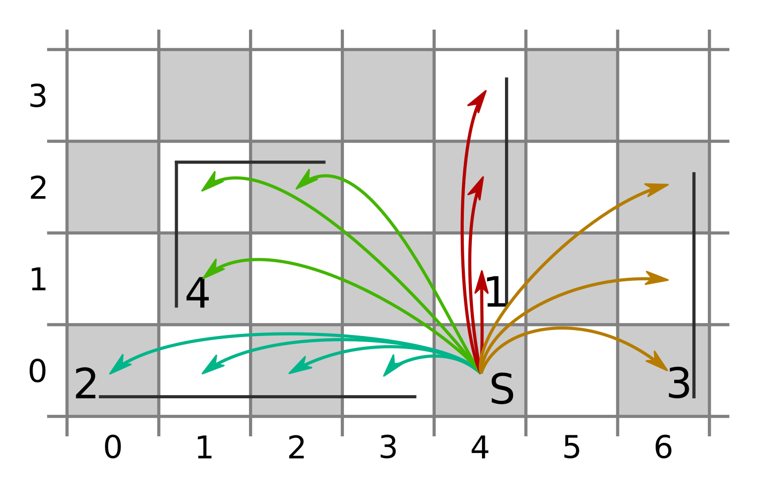
Figure 2: Schematic representation of the selected movement target positions on a grid with 10 cm spacing (see also Figure 1(b)). The start/end position is labeled S, the target positions are grouped into groups indicated by color and numbers.

II-A3 Extraction of the 3D trajectories

From the obtained movement recordings, we extracted the positions of the knuckles and wrist in the 2D images using DeepLabCut (DLC) [19], a neural network, which can be trained to track user-specified features in images and is publicly available as a python package [20, 21]. For the training of DLC’s neural network, we labeled 1000 frames out of all recordings. They were chosen by DeepLabCut using its internal clustering algorithm for extraction of the most differing frames in the respective videos. The error in feature tracking obtained from the test set is around three pixels. This corresponds to up to 5 mm distance, depending on the position of the hand in the camera frame. An error of 5 mm corresponds roughly to the size of the knuckles, which are inherently not very strictly defined features.

After 2D tracking, we reconstructed the 3D positions of those features using anipose [22], a publicly available 3D reconstruction library which is specifically built to work with DeepLabCut [23]. We used its spatiotemporally constrained triangulation method for the reconstruction of the 3D trajectories. It introduces additional terms in the triangulation loss function that penalize behavior that is possible in general, but not in the special case of hands. Tracked points may not accelerate arbitrarily fast (hands have mass) and their relative position cannot change arbitrarily, because hands have a given physical structure. To obtain the final trajectories used in this work, we averaged the trajectories of the four knuckles and the wrist into one general hand position.

II-B Dynamical Movement Primitives

II-B1 Model description

The framework of Dynamical Movement Primitives (DMPs) [4, 24] is formalized by a system of second order differential equations. They consist of a critically damped linear attractor system and a non-linear forcing term to make the attractor follow a desired trajectory. The forcing term is learned from the presented data. The DMP model is a 1D system, so three separate models need to be trained for 3D trajectories, one for each dimension.

Here we use the DMP version introduced by [25]. It has been shown to have equivalent overall performance as compared to the original Ijspeert formulation [26], but better convergence at the end- and joining-point of the movement trajectory. Since in this work we do not analyse joining of movement trajectories, we removed the parameter $v$ from the model. In Appendix A-A we show that this modification does not significantly change the model’s performance. The differential equations for the dynamical system are:

$$\tau\dot{z} =\alpha_{z}(\beta_{z}(r-y)-z)+f$$ (1)

$$\tau\dot{y} =z$$ (2)

$$\tau\dot{r} =\frac{\Delta_{t}}{T}\,(g-s).$$ (3)

Here $s$ and $g$ are the start- and end-points of the trajectory, $\alpha_{z},\beta_{z}$ and $\tau$ are constants of the dynamical system, which in this study were set to $\alpha_{z}=0.75$, $\beta_{z}=0.1875$, $\tau=1$ to make the attractor system critically damped (no oscillations). Parameters $T$ and $\Delta_{t}$ are duration and sampling rate of the trajectory.

The time series of the variables $z$ and $y$ encode the velocity and position of a trajectory and can be obtained by integrating the system. The forcing term $f$, that encodes the trajectory, is represented as a linear combination of $K$ Gaussian kernels $\psi_{i}$ with weights $w_{i}$:

$$f =\frac{\sum_{i=1}^{K}\psi_{i}w_{i}}{\sum_{i=1}^{K}\psi_{i}}$$ (4)

For this work, we chose the kernels to be equally spaced in time with their centers $c_{i}$. Furthermore, we do not learn the individual standard deviations $\sigma_{i}$, but set them to scale with the number of kernels $K$ as

$$\sigma=\frac{\kappa}{K},$$ (5)

with some optimal $\kappa$ determined from data (see Appendix B-A). This means, the more kernels there are, the narrower they get, hence the sum of the standard deviations $\sigma_{i}$ remains fixed at $\kappa$.

The only individually learned parameters in this model are the weights $w_{i}$. To learn the weights, locally weighted regression [4] is used widely, but any other supervised learning rule can be used, too. Here we used the simple $\delta$-learning rule [27]

$$\Delta w_{i}=\mu\left(\gamma(c_{i})-y(c_{i})\right)$$ (6)

where $\gamma(c_{i})$ and $y(c_{i})$ denote the target trajectory to be encoded and trajectory generated by the model at the position of the $i$-th kernel, respectively. Parameter $\mu$ denotes the learning rate. The process $w_{i}\leftarrow w_{i}+\Delta w_{i}$ has to be repeated sufficiently many times until the weights converge. For our evaluation we used 200 training iterations with a learning rate of $\mu=0.1$.

The number of free parameters in the model is just the number of weights, which is equal to the number of kernels $K$. With one weight vector for each dimension $D$ we get $n_{\text{DMP}}=DK$ for the number of free parameters. In our case of $D=3$ this yields

$$n_{\text{DMP}}=3K.$$ (7)

II-B2 Generalization using DMPs

The simplest way to generalize to a new situation is to change the start $y_{0}$ or goal point $g$ of the DMP [4] which also scales the trajectory accordingly based on the distance between the original and new star-/end-point. However, this uniform scaling is not well suitable in all cases. Consider a situation as given in 3(b) (b). The put on top trajectories all rise about 3 cm above the end-point height before the object is set down, regardless of the actual end-point height. If one would simply change the DMP goal point of the lowest trajectory to the highest end-point to achieve a generalization, the trajectory component for height would just scale accordingly (approximately by the factor of three, since the highest point is about three times higher). This scaled trajectory would therefore rise around 9 cm higher above the goal point before going down to reach the end-point, which would deviate by far (instead of the observed 3 cm) from the human demonstration trajectory.

To achieve a generalization closer to the human trajectory, we instead take a weighted average of the DMP weight vectors $\bm{w}_{n}$ of nearby demonstrations. The weights $\alpha_{n}$, are obtained by the following process. First, we shift every trajectory to start point $y_{0}=0$. Then, we express the new goal $g_{\text{new}}$ as a linear combination of the demonstration goals $g_{n}$

$$g_{\text{new}} =\sum\alpha_{n}g_{n}$$ (8)

with averaging weights $\bm{\alpha}=(\alpha_{1},...,\alpha_{n})$. This equation is underdetermined, so we add the additional constraints

$$\sum\alpha_{n} =1\text{ and }||\bm{\alpha}||\text{ minimal.}$$ (9)

Minimizing the norm of $\bm{\alpha}$ forces the demonstrations to contribute as equally as possible to the weighted sum. This selects the one solution where all demonstrations contribute as much as individually possible to obtain the target trajectory (using the most of the available information), while still optimizing for giving more weight to the trajectories of highest relevance. Else, as the system is heavily under-determined, it could be that only a few of the given demonstrations are considered at all.

Furthermore, we take an unweighted average over the dimensions that we do not change in the generalization. The variation in the $g_{n}$ of those dimensions only comes from the demonstration variance and does not imply that the situation changed and some trajectories should contribute more.

Because of this mode of generalization, there is no fixed number of free parameters. Instead it depends on the number of demonstration encodings used, which each contribute $3K$ parameters according to Equation (7). After averaging, the model again only contains $3K$ parameters, but cannot generalize to new situations on its own.

In addition to the main comparison between the three different models, we also performed a comparison between three different DMP generalization schemes: 1) change of the end-point, 2) weighted distance averaging, and 3) weighted goal averaging with constraints (as explained above). For the results of this comparison please see Appendix A-B).

II-C Task Parameterized Gaussian Mixture Models

II-C1 Model description

Gaussian Mixture Models (GMMs) are generally used for regression of arbitrary $D$-dimensional distributions. A GMM performs regression on a general distribution $\bm{\xi}_{t}$ (with $t=1,...,N$ datapoints) by approximating it with a linear combination of $i=1,...,K$ multivariate Gaussian kernels $\mathcal{N}_{i}(\bm{\mu}_{i},\bm{\Sigma}_{i})$. Here, $\bm{\mu}_{i}$ is the mean of a Gaussian (vector of length D), and $\bm{\Sigma}_{i}$ its variance ($D\times D$ matrix). The linear combination coefficients are called $\pi_{i}$ and fulfill $\sum_{i}\pi_{i}=1$.

There are multiple ways to encode trajectories using GMMs [9, 13, 7, 8]. In this work, we used the method called time-based Gaussian Mixture Regression (tbGMR, [9]), which will be described in Section II-C2. This approach in itself can only encode trajectories and is unable to generalize from demonstrations to new situations. To allow for that, a model called Task Parameterized GMM (TP-GMM) [9] is used. This model fits multiple models with the tbGMR approach simultaneously and combines them to a single model. Note that the TP-GMM approach is also able to support different kinds of GMM encodings. For our analysis, we used a Matlab / Gnu Octave implementation of the model provided by [9].

II-C2 Time based GMR

For time-based GMR, the joint distribution $\mathcal{P}(\bm{\xi}^{I}_{t},\bm{\xi}^{O}_{t})$ of time $\bm{\xi}^{I}_{t}$ (superscript $I$ for input) and the spatial coordinates $\bm{\xi}^{O}_{t}$ (superscript $O$ for output) at that time is encoded. Note that, in contrast to DMPs, time is treated as an additional input dimension to the model, not as an independent variable.

To reconstruct the encoded trajectory, the conditional probability of having spatial coordinates $\bm{\xi}_{t}^{O}$ at a given time $\bm{\xi}_{t}^{I}$, $\mathcal{P}(\bm{\xi}^{O}_{t}|\bm{\xi}^{I}_{t})$, is used. Mathematical details on how to obtain it from $\mathcal{P}(\bm{\xi}^{I}_{t},\bm{\xi}^{O}_{t})$ are given in [9] in Section 5.1. With some simplification, this distribution is again a multivariate Gaussian for each $\bm{\xi}_{t}^{I}$. Thus, we can take the centers $\hat{\bm{\mu}}_{t}^{O}$ as the predicted trajectory of the model. Furthermore, the values of $\hat{\bm{\Sigma}}^{O}_{t}$ contain additional information about the uncertainties in the model, as they define uncertainty-ellipsoids around the predicted positions. Such information can, for example, be used in robotic applications, to indicate how strongly a motion controller should enforce following the predicted trajectory of the $\hat{\bm{\mu}}_{t}^{O}$.

To avoid overfitting, the model has to be regularized. The implementation we used in this work realizes this by adding a small constant $\epsilon$ to the main diagonal of the covariance matrices after each M-step in the fitting algorithm. More information on this is given in Section II-C3. This reduces their capability to get too restrictive in individual dimensions, smoothing out the obtained trajectories.

The parameters used by tbGMR are

$$\left\{\pi_{i},\bm{\mu}_{i},\bm{\Sigma}_{i}\right\}_{i=1}^{K}.$$ (10)

The number of parameters depends on the number of Gaussians $K$ and the data dimension $D$. Since the $\bm{\Sigma}_{i}$-matrices are symmetric, they have $(D^{2}-D)/2+D$ free parameters each (the upper right triangle including the diagonal). The $\bm{\mu}_{i}$ each contain $D$ free parameters. From the $K$ linear combination coefficients $\pi_{i}$ only $K-1$ are free, because of the normalization condition $\sum_{i}\pi_{i}=1$. Thus, we have

$$n_{\text{GMM}}=K\left(\frac{D^{2}-D}{2}+2D\right)+K-1$$ (11)

free parameters in total. In the case of 3D-trajectories, this model is 4-dimensional (one additional time dimension). Therefore, setting $D=4$ into Equation (11), we get

$$n_{\text{tbGMR}} =15K-1$$ (12)

for the number of free parameters in the model.

II-C3 Task parameterized GMM

A TP-GMM considers the data $\bm{\xi}$ in different reference frames $j=1,...,P$. They are obtained by affine linear transformations with some rotation matrices $\bm{A}_{j}$ and translation vectors $\bm{b}_{j}$. Those are called the “Task Parameters”, because they parameterize the relation of the different reference frames for each demonstration (task). GMMs in all reference frames are fitted to the data using the Expectation-Maximization-Algorithm (EM-Algorithm, [28]) in a modified version to fit all reference frames simultaneously (see Appendix A in [9]).

The models in the different reference frames $P$ can be combined to one model from which a trajectory can be retrieved by means of the chosen encoding type. Its means $\hat{\bm{\mu}}_{i}$ and covariances $\hat{\bm{\Sigma}}_{i}$ are obtained as

$$\hat{\bm{\Sigma}}_{i} =\left(\sum_{j=1}^{P}\left(\hat{\bm{\Sigma}}_{i}^{(j)}\right)^{-1}\right)^{-1},$$ (13)

$$\hat{\bm{\mu}}_{i} =\hat{\bm{\Sigma}}_{i}\sum_{j=1}^{P}\left(\hat{\bm{\Sigma}}_{i}^{(j)}\right)^{-1}\hat{\bm{\mu}}_{i}^{(j)}$$ (14)

$$\mathrm{with}\;\hat{\bm{\mu}}_{i}^{(j)}= \bm{A}_{j}\bm{\mu}_{i}^{(j)}+\bm{b}_{j}\;\mathrm{and}\;\hat{\bm{\Sigma}}_{i}^{(j)}=\bm{A}_{j}\bm{\Sigma}_{i}^{(j)}\bm{A}_{j}^{T}.$$ (15)

The ability to generalize to new situations is introduced by combining the models of the different reference frames with different task parameters than the ones used during learning. Note that the individual GMMs in the two different reference frames encode something conceptually different from a standard GMM with one reference frame. They cannot be used individually to retrieve the encoded trajectories, since they represent a combination of all learned trajectories as seen from one reference frame only.

If no generalization is needed, we set $P=1$, let $\bm{A}_{1},\bm{b}_{1}$ define the identity transformation and a TP-GMM simplifies to a GMM in only one reference frame without generalization capabilities. The usage of $P$ different reference frames leads to $P$ sets of $\bm{\mu}_{i}^{(j)},\bm{\Sigma}_{i}^{(j)}$ in the model instead of one.

It is possible to take different kinds of GMMs for encoding and reconstruction and enable generalization via the TP-GMM approach. Here we used time based Gaussian Mixture Regression as explained in Section II-C2 to encode trajectories. Thus, we have

$$n_{\text{TP-GMM}}=KP\left(\frac{D^{2}-D}{2}+2D\right)+K-1$$ (16)

free parameters in total. This only differs from Equation (11) by the factor of $P$ in the first term reflecting the additional sets of $\bm{\mu}_{i}^{(j)},\bm{\Sigma}_{i}^{(j)}$. In this work we will use $P=2$, so putting in $D=4$ from out tbGMR approach and $P=2$ we get

$$n_{\text{TP-GMM}} =29K-1$$ (17)

free parameters for a TP-GMM.

II-C4 Generalization using TP-GMM

In contrast to the DMP framework, where generalizations can be obtained by combining the weights of existing encodings for single trajectories, the TP-GMM approach operates on new encodings of multiple demonstration trajectories.

To generalize from a set of demonstrations to a new situation, we encode a TP-GMM with two reference frames $P=2$ We chose the Task Parameters such that they rotate and translate all demonstration trajectories into two reference frames defined as follows: In the first frame, identified by $j=1$, all trajectories begin at $\bm{0}$. Furthermore, they are rotated such that their end-point lies in the yz-plane. In the second frame, denoted by $j=2$, the roles of start- and end-point are switched. This yields $\bm{A}_{j}^{O}$ and $\bm{b}^{O}_{j}$ (O for output dimension as above) that define the 3D affine transformations to the reference frames. The time dimension, however, is kept invariant under the transformation of the task parameters. Therefore, the variables $\bm{A}_{j}$ and $\bm{b}_{j}$ for the TP-GMM, become

$$\bm{b}_{j}=\begin{bmatrix}\bm{0}\\ \bm{b}^{O}_{j}\end{bmatrix},\ \bm{A}_{j}=\begin{bmatrix}\bm{1}&\bm{0}\\ \bm{0}&\bm{A}_{j}^{O}\end{bmatrix}.$$ (18)

To generalize to a new trajectory, the recombination to one GMM is done with $\bm{A}_{j}$ and $\bm{b}_{j}$ of the target trajectory. These are obtained in exactly the same way as for the demonstration trajectories. The resulting GMM encodes a prediction for a trajectory with the new Task Parameters, which can be extracted by means of the encoding method used.

II-D Stable Estimator of Dynamical Systems (SEDS)

II-D1 Model description

The SEDS model [8], like the DMP approach, considers the trajectory to be the time evolution of a nonlinear dynamical system. In the case of SEDS it takes the simple form

$$\dot{\bm{\xi}}=\bm{f}(\bm{\xi})$$ (19)

where $\bm{\xi}$ is the position in state space and $\bm{f}$ some multi-dimensional nonlinear function. Trajectories cannot cross in state space, so care needs to be taken when choosing the state space variable $\bm{\xi}$. In this work we used position and velocity. The function $\bm{f}$ gets approximated by a GMM analogous to the time based GMR method from Section II-C2. The joint distribution $\mathcal{P}(\bm{\xi},\dot{\bm{\xi}})$ is encoded with a GMM. For given $\bm{\xi}$, $\dot{\bm{\xi}}$ is then extracted as the maximum of the conditional probability $\mathcal{P}(\dot{\bm{\xi}}|\bm{\xi})$.

In general, there exist several methods to estimate the parameters of the GMM (see Figure 3 in [8]), but they all have problems with stability. It is, thus, not guaranteed that a reconstructed trajectory will converge to the goal position in case of GMM.

The core of the SEDS approach is its way of estimating $\bm{f}$. With SEDS, it is guaranteed that there is only one global attractor in the dynamic system, that is asymptotically stable, so trajectories from every point will converge to it. This property is achieved by reformulating the estimation of the GMMs parameters as a constrained nonlinear optimization problem optimizing model accuracy under the constraint of global asymptotic stability. The exact formulation of the optimization problem is given in Section V in [8]. As shown in Figure 3 in [8], the SEDS optimization leads to a smooth phase space with no secondary attractors. There, two different measures for model accuracy were proposed, the likelihood of the model and the mean squared error (MSE) of its prediction to the demonstration. In this work, we used the MSE. [8] also provides an implementation of the algorithms, which we used for our analysis.

While the the resulting model is guaranteed to converge to the goal state, the nonlinear optimization to fit the model is not guaranteed to succeed. We start from an estimation obtained by conventional GMM regression with the EM-algorithm, modify it to fulfill the constraints, and then refine it with SEDS optimization. If optimization fails, we add noise to the initial conditions and start the optimization again. Additionally, after five failed trials, we increase the value of the tol_mat_bias value in the SEDS optimizer, that is similar to the $\epsilon$ of the TP-GMM models and is documented by the authors of the SEDS code as helping with instabilities. We consider an optimization as failed if the numeric solver reports a fail or if the obtained model is unable to reconstruct the first given demonstration trajectory with less than 2 cm distance anywhere along the trajectory or 5 mm at the end point. Note that we do not test the model against the generalization target to judge if the optimization should be repeated, which, unfairly, would use test data for training, but compare against data that was already used in training.

The number of free parameters in a SEDS model optimized with the MSE-loss is $K(1+\frac{2}{3}D(D+1))$ [8]. For our state space dimensionality of $D=6$ (position and velocity) this yields

$$n_{\text{SEDS}}=29K.$$ (20)

II-D2 Movement generalization

Since SEDS optimization yields a globally stable attractor, one can simply change the position of the starting point of the integration to obtain a new trajectory that will converge to the target. While the model is designed to yield trajectories similar to the demonstrations in a vicinity around them, it is unclear whether its predictions will be accurate for generalization targets farther away. Therefore, the similarity between generalization and true human demonstrations will depend on the nature of the attractor landscape produced by the optimization. Furthermore, the duration of the movement cannot be set directly, but also depends on the properties of the attractor. In a first step we just integrate the dynamic system for as many timestamps as there are in the target trajectory (like we do with the other models). Additionally we also integrate the model for as many timesteps as needed to arrive within 5 mm of the target position, this distance corresponds to our estimated motion tracking accuracy in the dataset.

II-E Movement Encoding and Reconstruction

II-E1 Hyperparameter tuning

Choosing sub-optimal hyperparameters has different effects, depending on the type of model. The stability of the SEDS model is not considered here but in Section III-A2, because we don’t have direct influence on the kernel width in that model.

Both DMP and tbGMR will produce oscillations in the velocity profile, if the kernel width is too narrow in case of DMPs or the regularization term is too small in case of tbGMR. This is not the case for the human demonstrations. Choosing sub-optimal width for the DMP kernels increases the reconstruction error (see Appendix B-A). For tbGMR, however, lowering the regularization, and therefore introducing oscillations in the velocity profile, reduces the reconstruction error of the position profile. This makes choosing hyperparameters more difficult, as the well defined reconstruction error cannot be the only criterion (see Appendix B-B). Therefore it is harder to determine the optimal regularization for accurate but still human-like trajectories with the tbGMR model.

II-E2 Evaluation procedure

To test the reconstruction capabilities of the different models, we encoded every single trajectory from our dataset with every model, varying the number of kernels used from $K=3$ to $K=11$ for DMP and tbGMR and from $K=3$ to $K=7$ for SEDS. In case of SEDS, we did not use higher $K$ values as for the other models, since the encoding times due to the optimization process became unreasonably long. The respective hyperparameters of the model were chosen optimally, detailed information on this is given in appendix B. We also investigated the influence of sub-optimally chosen hyperparameters on the reconstructions, because sensible output for a wider region of hyperparameters means better usability of the model.

II-E3 Performance measures

To assess the error in the reconstructions, we computed the root mean squared distance $d$ between the reconstruction $r$ and the original trajectory $o$ for every reconstruction as

$$d=\sqrt{\frac{1}{N}\sum\limits_{i}^{N}(r_{i}-o_{i})^{2}}.$$ (21)

The resulting distributions of errors are not normally distributed, but skewed and contain a tail of more inaccurate reconstructions. Therefore we use medians instead of means to represent the average error in the reconstructions of the different models.

II-F Movement Generalization

II-F1 Hyperparameter tuning

As we only recombine existing DMP encodings for generalization, hyperparameter tuning does not have to be reconsidered for this model.

However, the tuning of the TP-GMM hyperparameters need to be tuned again, since the fitting process is different from the reconstruction case (see Section II-C4). We observed the same qualitative behaviour as in the reconstruction case. Lowering the regularization term reduces the error of position profile, but increases oscillations in the velocity profile. To obtain smooth trajectories, the regularization term had to be chosen an order of magnitude higher than in the reconstruction case. However, this lead on average to more than 5 mm error at the end-point of the trajectory regardless of the number of kernels.

To circumvent this issue, we chose to use only little regularization ($10^{-6}$) and removed the oscillations by filtering the high frequencies out with a low-pass filter at 3 Hz. While this is a post-processing step that is not part of the model, it is neither complex nor computationally expensive.

II-F2 Evaluation procedure

To test the generalization capabilities of the models, we presented specific subsets of the dataset (training set) as demonstrations for encoding and then used the generalization methods described above to generate trajectories for new situations obtained from remaining trajectories in the dataset (test set). This way we can directly compare the model predictions to the trajectories of human demonstrations.

We tested two different generalization scenarios with different selection of demonstration trajectories. In the first case we only used two trajectories of one action type to generate a new trajectory. This represents the case where only few demonstrations are available. For this, we selected triplets of start-/end-points that were orthogonally connected (see Figure 2). We then interpolated from the outer demonstrations to the inner one and extrapolated from the inner and one of the outer demonstrations to the respective other outer demonstration. For example, using the indexing from Figure 2, we extrapolated from moves to positions (1,0) and (1,1) to a move to (1,2). Because we have three repetitions of each action type, this means the models get 6 demonstration trajectories (two sets of three instances of the same class) to generate the new target trajectory.

In the second case we used all available demonstrations for a specific action type, but excluded the generalization targets and everything that ends closer than 3 cm to the generalization target’s end point. For the TPGMM-model we further excluded all demonstrations that were closer than 3 cm to the target position in the TPGMM reference frame, otherwise, trajectories for positions with the same length over ground (for example (2,2) and (6,2), see Figure 2) would have provided direct demonstrations for the generalization target.

In both cases we did not use demonstrations from multiple participants in one model, every generalization task was done for each participant individually.

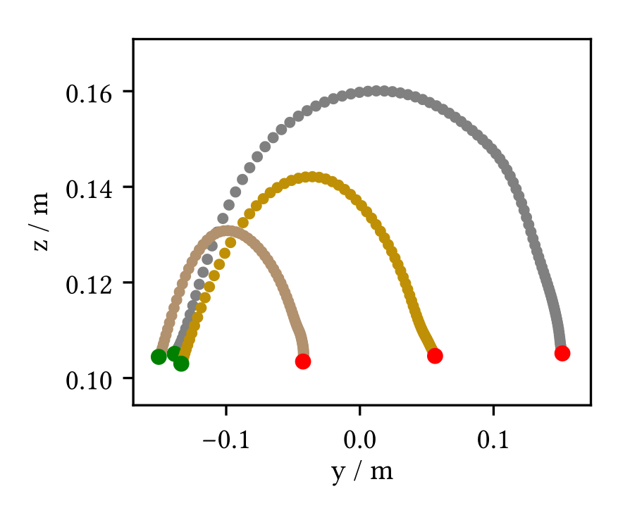
(a) Pick and place to
different target positions.

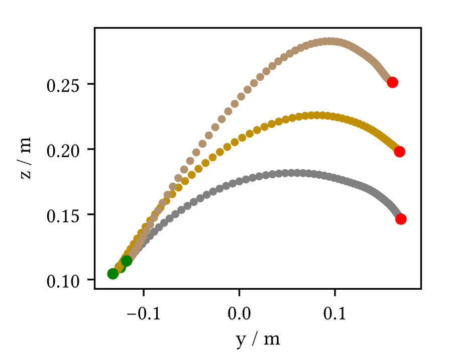
(b) Put on top of objects
with different heights.

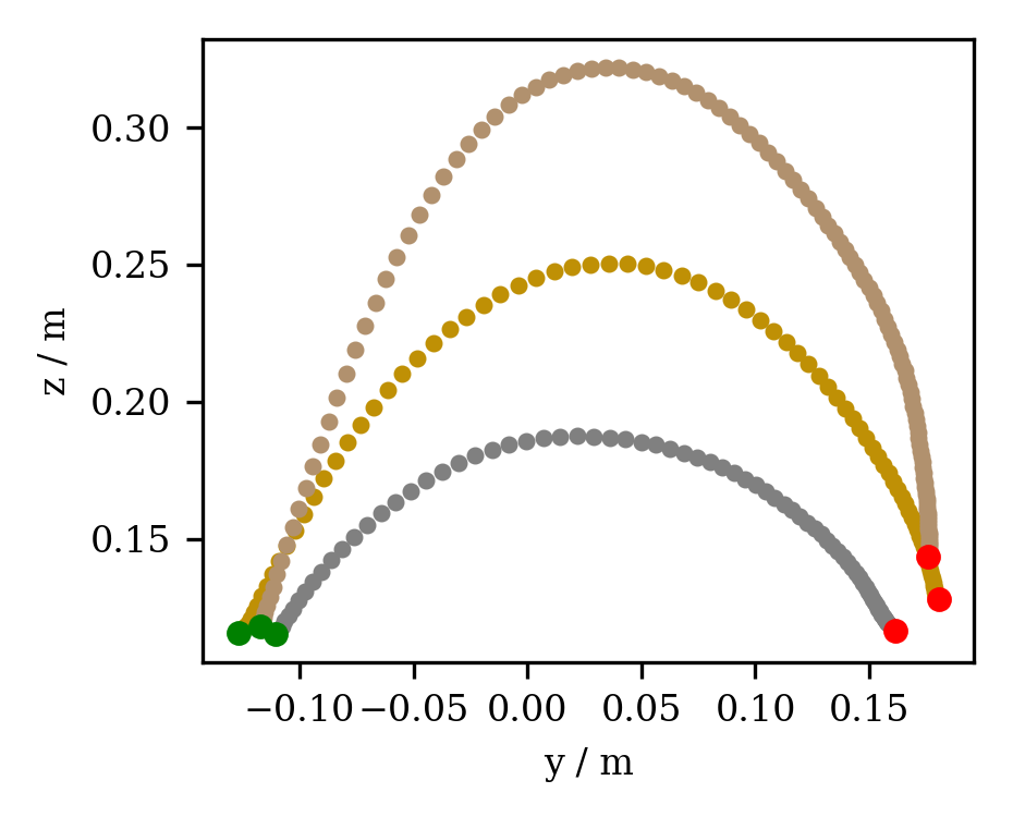
(c) Put inside objects
with different heights.

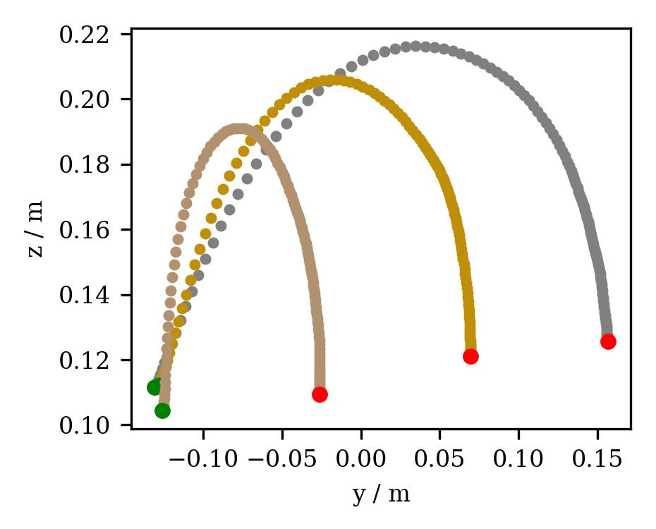
(d) Hide to different
target positions.

Figure 3: Examples of trajectories from the movement dataset. Green and red dots denote start- and end-points, respectively.

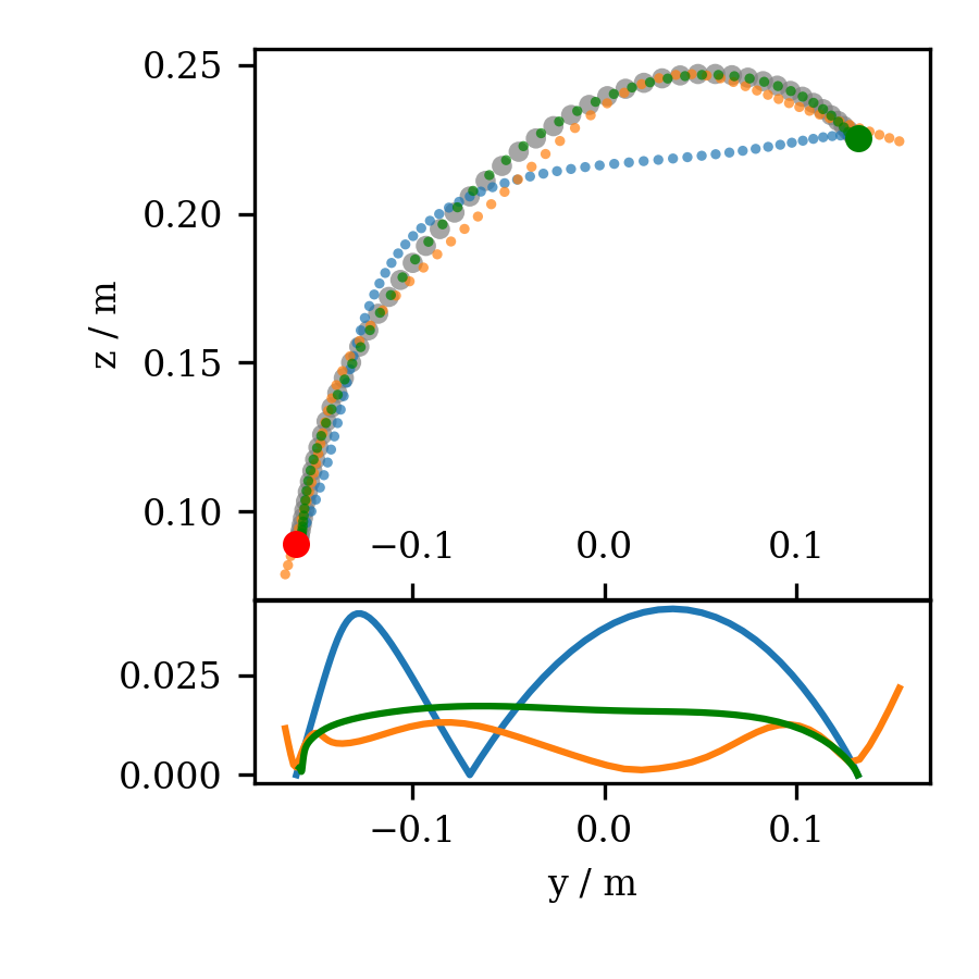
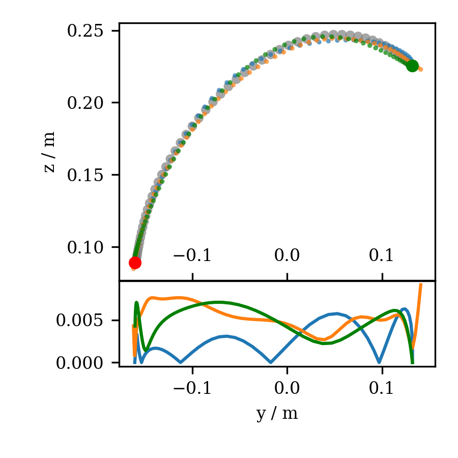
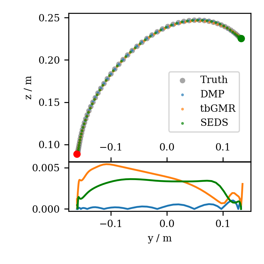
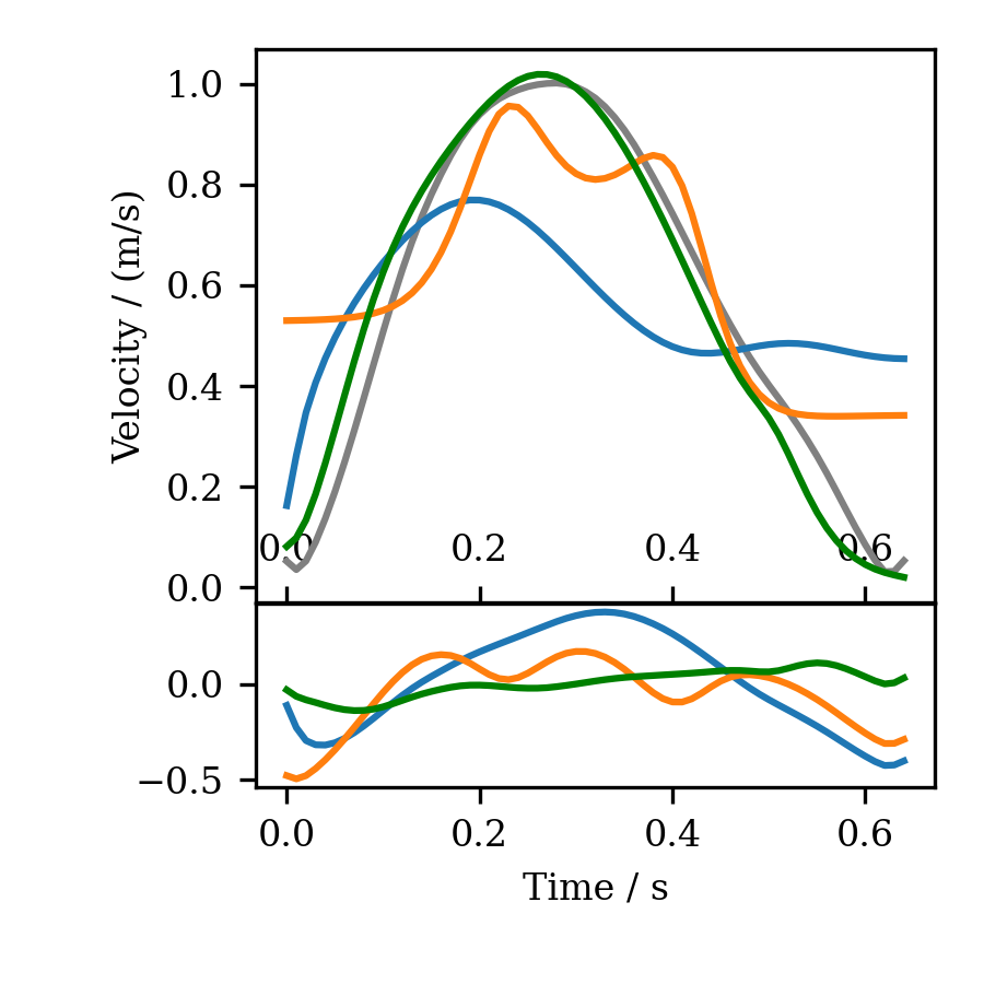
(a) 3 kernels.

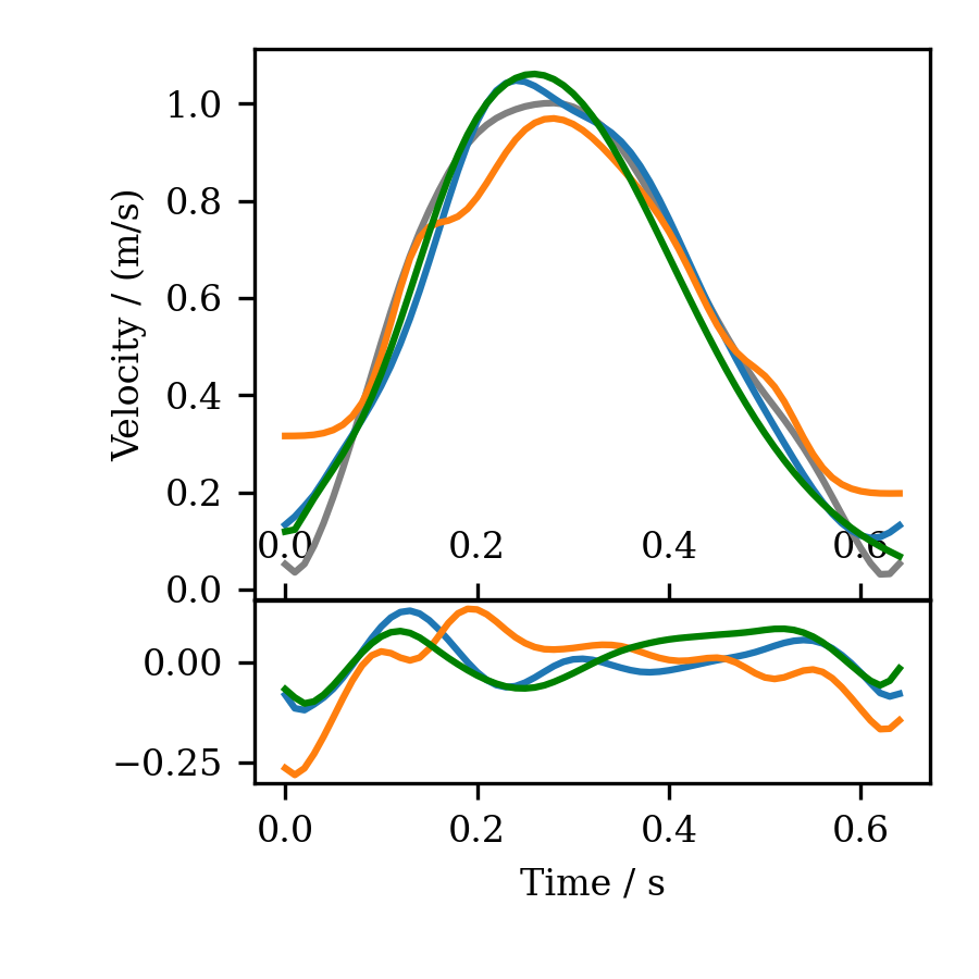
(b) 6 kernels.

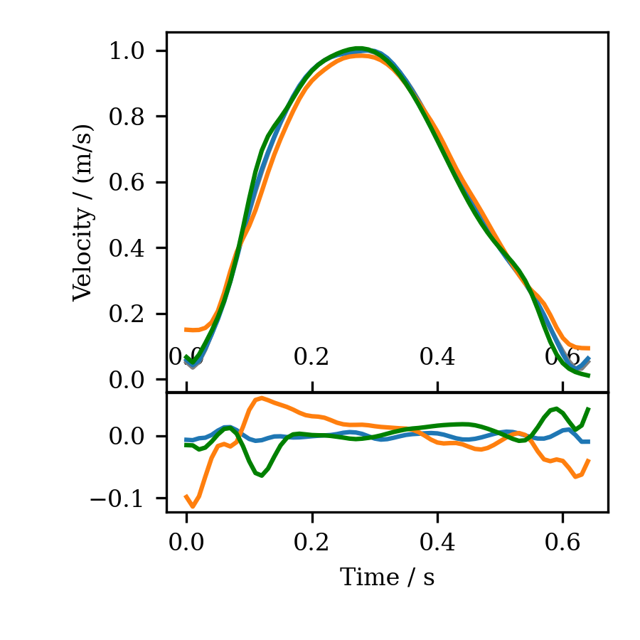
(c) 11 kernels.

Figure 4: Example of human trajectories of a take down action and reconstructions for different numbers of kernels: 3 (a), 6 (b) and 11 (c). Position and velocity profiles are shown in the top and bottom rows, respectively, whereas the plots at the bottom of each panel show the deviation from human the trajectory. Green and red dots denote start- and end-points, respectively.

II-F3 Performance measures

As in the case of trajectory reconstruction, the main measure to assess the generalization quality is the deviation of the generalized trajectory from the human target demonstration. We use the same measure as before, given in Equation (21). To gain a more complete picture of the model performance, we used two additional measures for further comparison.

We compared the deviation of the generalization from the true demonstration with the general variance in the dataset itself. This helps to qualify meaning of the deviation between generalized and ground truth (human) trajectory, since identical trajectories (as in reconstruction) are not expected. It is possible to do this, because we have three repetitions of every single action. So to estimate the variance in the human execution of the actions, we measured the mean squared distances $d_{h}$ between the individual human repetitions $h^{(j)}$ as

$$d_{h}^{(j,k)}=\sqrt{\frac{1}{N}\sum\limits_{i}^{N}(h^{(j)}_{i}-h^{(k)}_{i})^{2}}.$$ (22)

To compare the trajectories of different lengths, we down-sampled the longer trajectory to match the shorter trajectory.

Note that $d$ and $d_{h}$ are conceptually different measures. $d$ measures error between a human trajectory and the corresponding generalized trajectory, whereas $d_{h}$ measures variance in the human repetitions. The end-points of the human trajectories were not given, because humans grasped the object slightly differently in different repetitions, resulting in differences between the repetitions. The model generalizations, however, are given exact start- and end-points. Therefore, the inter human variance for repetitions of a demonstration is conceptually different and expected to be higher than the distance between a generalized target trajectory and the corresponding human demonstration. We assume that the obtained generalization accuracy is reasonably acceptable if it does not exceed the variance of the human demonstrations.

The second measure we used for additional quantification was the end-point deviation $d_{e}$, defined as

$$d_{e}=\lVert r_{N}-o_{N}\rVert$$ (23)

with the predicted trajectory $r$ and the original trajectory $o$, both of length $N$. Here we assessed how close the end-points of the generalization come to the targets set by the human demonstration, regardless of the trajectory shape. This is to test the end-point convergence of the two GMM models.

Since the SEDS model does not always converge to the target position on time (see Section IV-A), we evaluated the generalization performance of SEDS for two cases: 1) under the condition with fixed trajectory duration (labelled SEDS in figures) as for the other models. Here, the fixed trajectory duration corresponds to the duration of the human demonstration. 2) under the relaxed condition on trajectory duration (labelled SEDS*). For this, we first did an estimation of acceptable time convergence. We measured how much longer the longest of the three repetitions of a human movement takes compared to the shortest one. We found that 95 % of all longest human demonstrations completed in less than 38 % more time than the shortest demonstration for the same task. Therefore, we counted a SEDS generalization successful under the relaxed time condition if it completed within 72.5 % and 138 % of the duration of the human demonstration and computed the generalization error only among those successful generalizations.

III Results

III-A Movement Encoding and Reconstruction

III-A1 Reconstruction accuracy

Some examples of human movement trajectories for several selected manipulation actions are shown in Figure 3, whereas Figure 4 shows some examples of trajectory reconstructions using different numbers of kernels. With only three kernels, all models but SEDS struggle with accurate trajectory representation. While tbGMR has the lowest overall error, the reconstruction clearly misses the correct start- and end-point. Although DMP has the largest overall error it has zero error at the start- and end-point, which is the outcome of the $\delta$-rule that we chose for the parameter learning. When increasing the number of kernels, the reconstructions become qualitatively identical to the demonstrations with errors dropping below the 5 mm of tracking error.

The median reconstruction error obtained from all reconstructions vs. the number of used kernels is shown in Figure 5.

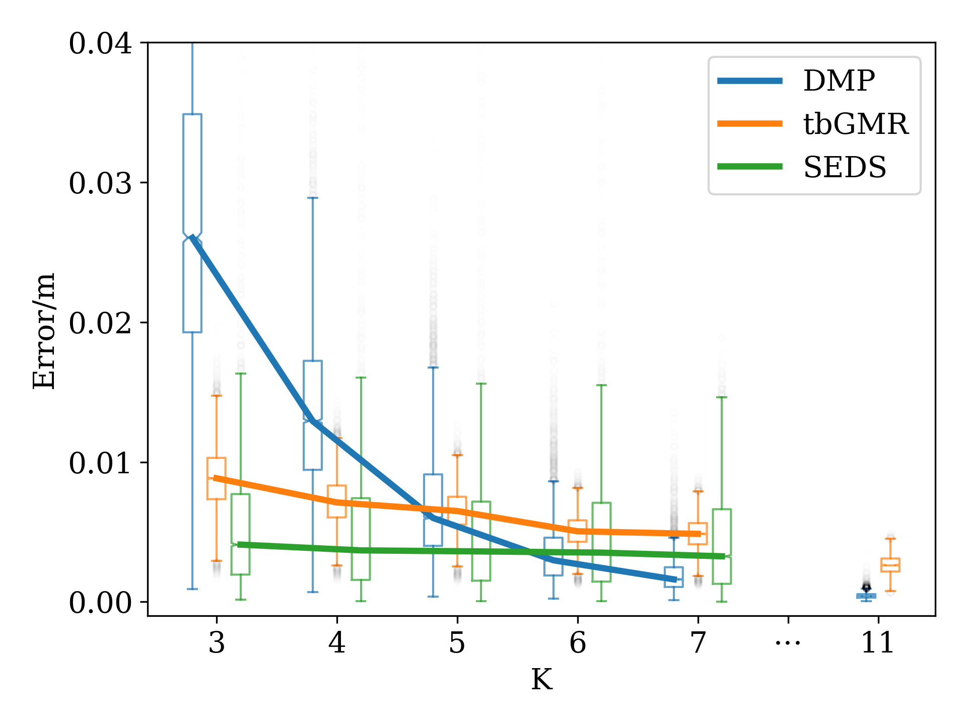
Figure 5: Comparison of movement encoding frameworks on the movement reconstruction task. Median reconstruction error vs. number of kernels is shown for each model. Failed SEDS encodings are not included this statistics (see Section III-A2). Note, there is no result for SEDS for $K=11$ because the encoding time for high $K$ values using the repeated optimization method (see Section II-D1) is impractically long.

We can see that the median errors of all models fall below our 5 mm tracking error estimate, if a sufficient number of kernels is used. However, there are qualitative differences among the three models. The DMP model performs worst for few kernels (three, four kernels) but becomes the best for more than six kernels, greatly benefiting from more kernels. SEDS and tbGMR improve less as compared to DMPs with the use of more kernels. Furthermore, the error distributions of DMP and tbGMR becomes much narrower, whereas the SEDS error only marginally decreases and the spread of the error distribution remains highest. This demonstrates that SEDS encoding can fail or be of insufficient reconstruction quality even with higher numbers of kernels. Moreover, increasing the number of kernels does not ensure convergence of the model. For the other two models, however, using more kernels significantly improves the reconstruction accuracy. Especially the DMP model becomes more and more accurate, reaching an error of 0.4 mm with $K=11$, whereas the tbGMR error is 2.6 mm.

Considering the parameters used to encode the trajectories (see Table III), the difference in using 1D or multidimensional Gaussian kernels (see Section IV-A) becomes apparent. Both GMM based approaches need many more parameters than the DMP regardless of the number of kernels. With $K=11$, DMP only needs 33 parameters, whereas the tbGMR and SEDS model with $K=3$ need 44 and 87 parameters, respectively. When comparing the two GMM based models, the tbGMR model uses fewer parameters, because the TP-GMM extension for generalization (that nearly doubles the parameters used) is not needed for reconstruction. Nevertheless, all encoding models compress the actual trajectory data (except for very short trajectories) significantly. The average length of a trajectory is 83 samples, which leads to $83\times 3=249$ parameters.

III-A2 Convergence of SEDS

As the optimization process in the SEDS model is not guaranteed to converge for all initial conditions, there were failed encodings. As described in Section II-D, we tried to mitigate this by adding random noise to the initial conditions and changing a parameter affecting stability. Still we were not able to find an automatic way to make the optimization convergent for all trajectories in the dataset regardless of the number of kernels $K$. With $K=3$, 84 % of the optimizations converged. The number of successful encodings increased with the higher number of kernels up to 92 % for $K=7$. Out of all trajectories, only 28 could not be successfully encoded regardless of the number of kernels. In almost all of the cases these trajectories were take out actions from the highest target object, which are also much longer as compared to the other actions.

III-B Movement Generalization

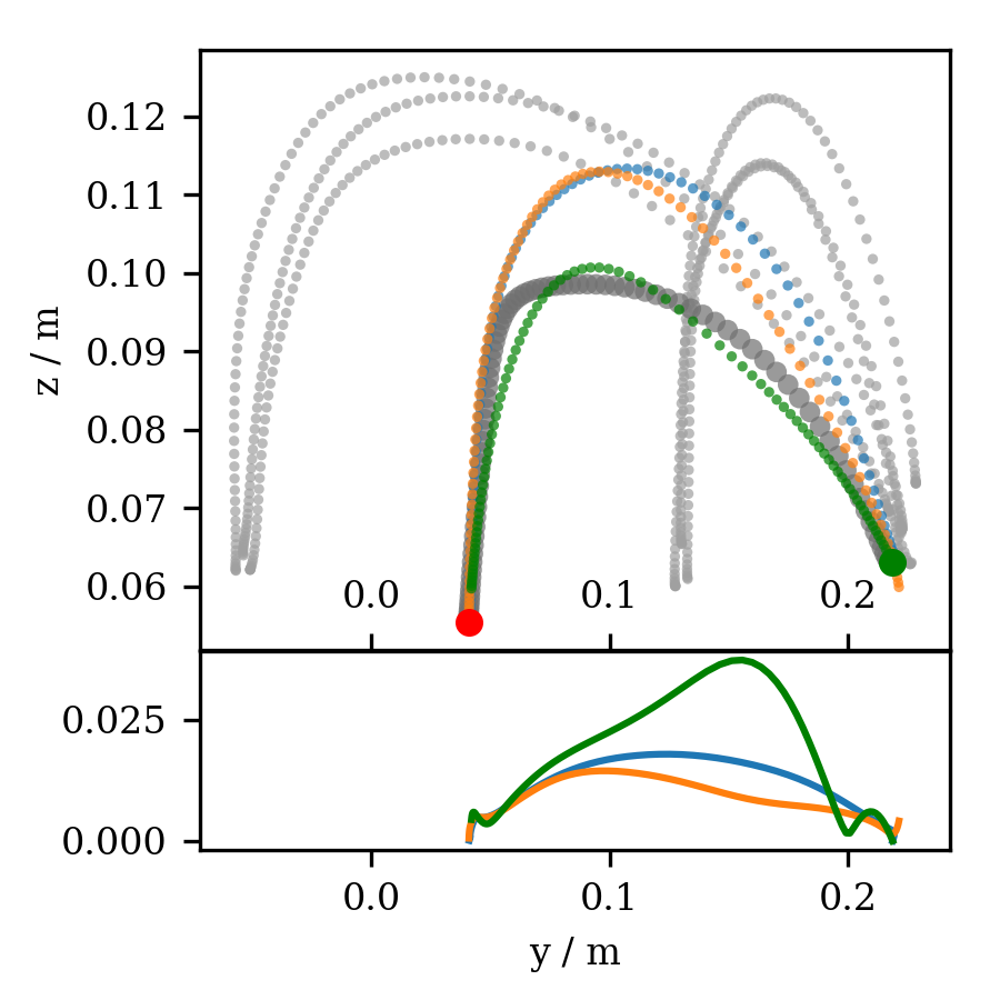
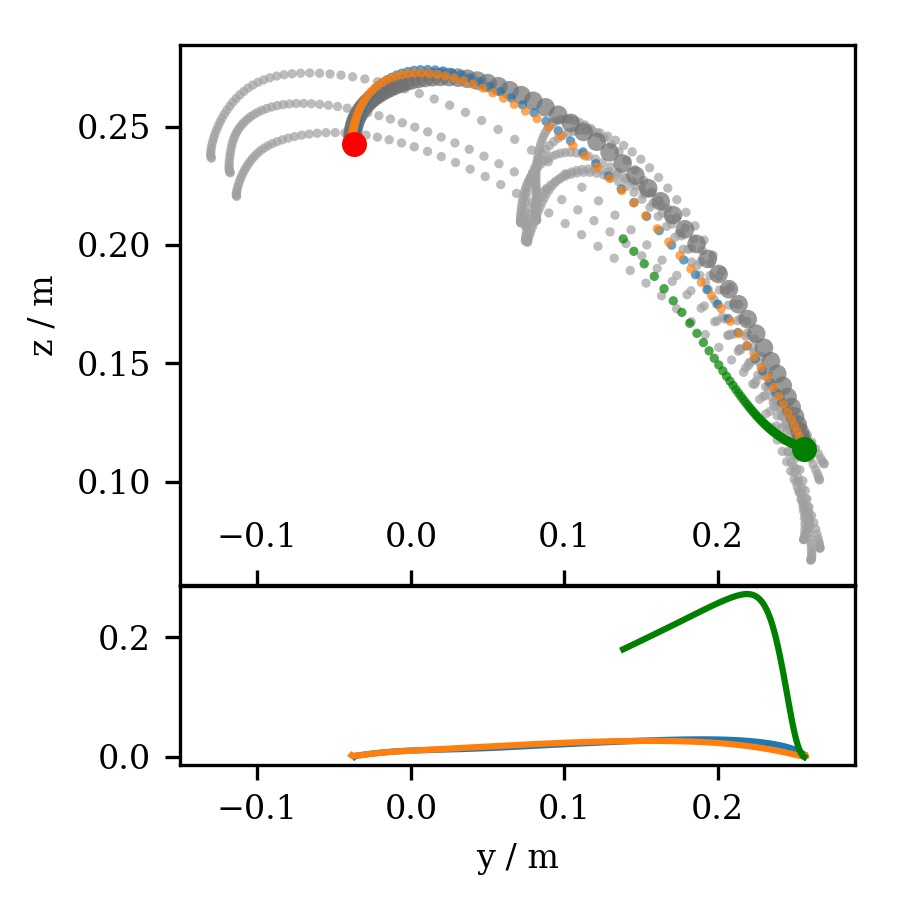
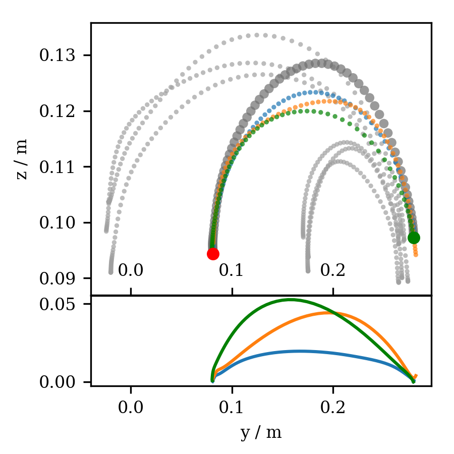
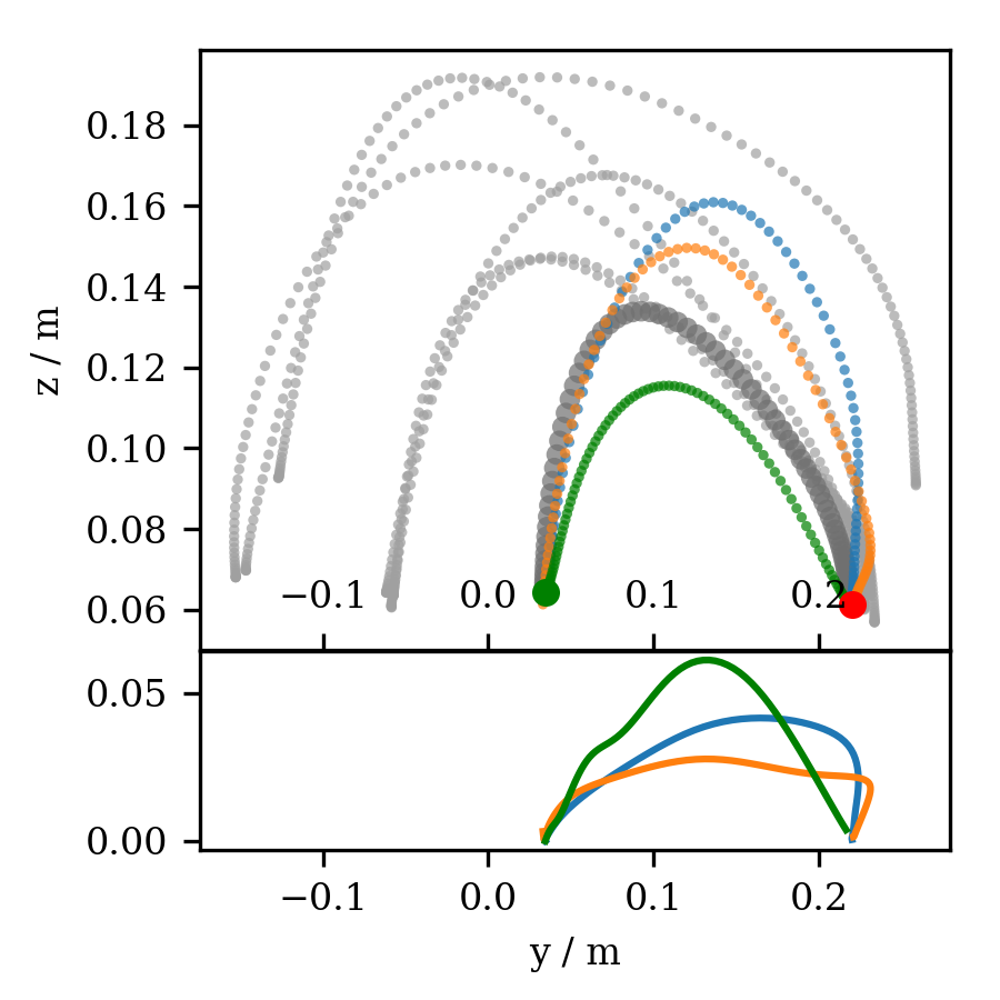
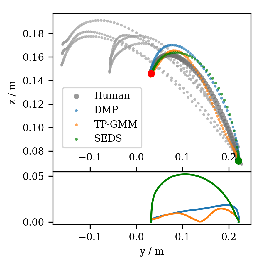
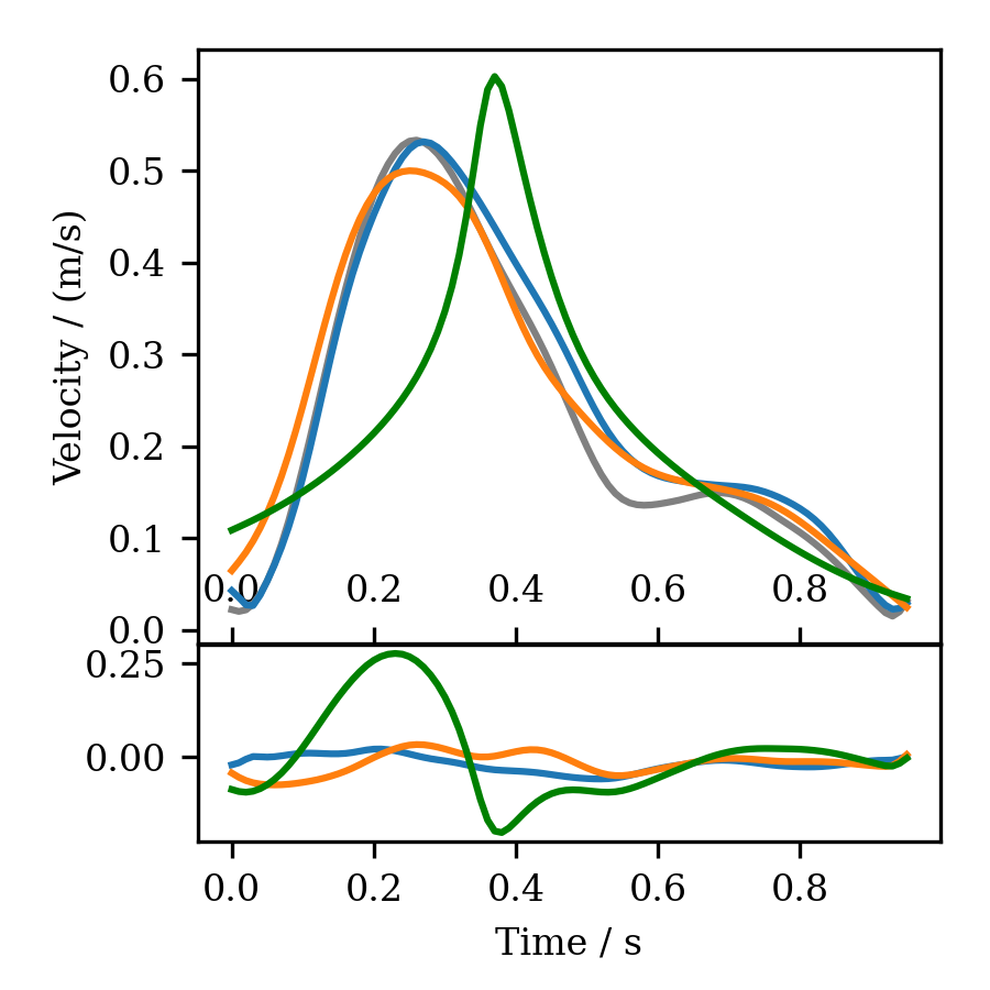
(a) hide,
interpolation

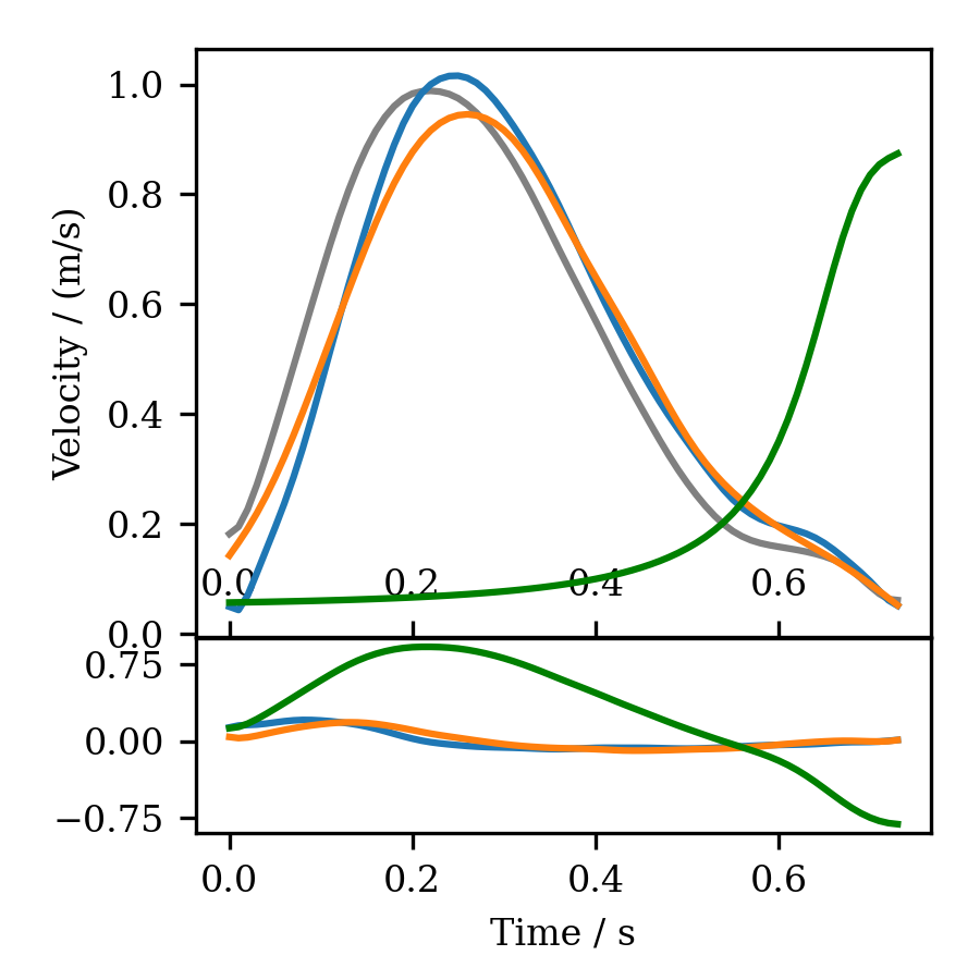
(b) put on top, red bucket,
interpolation

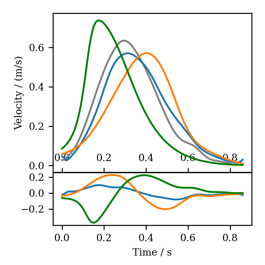
(c) pick and place,
interpolation

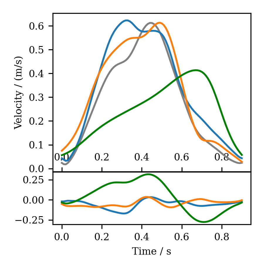
(d) uncover,
extrapolation

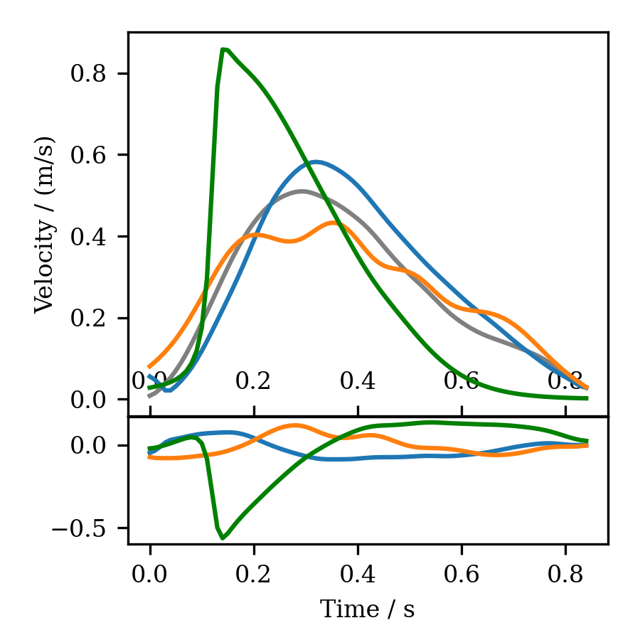
(e) put on top, blue bowl,
extrapolation

Figure 6: Examples of trajectories for different generalization situations. Position and velocity profiles are shown in the top and bottom rows, respectively, whereas plots at the bottom of each panel show the deviation from human trajectory. Color coding for models is the same as in Figure 4. Additionally, human demonstration trajectories are shown in light gray.

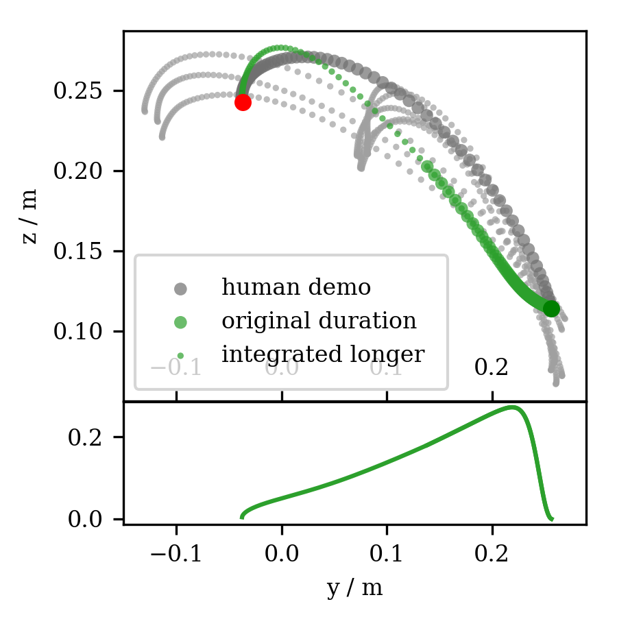
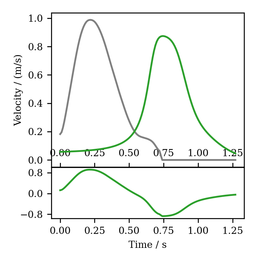
Figure 7: Generalization with the SEDS model for the put on top action from Figure 6(b) when integrating the model longer than the original duration of the human demonstration. Position and velocity profiles are shown on the left and the right side, respectively, whereas plots at the bottom of each panel show deviation from human trajectory.

III-B1 Generalisation using only few demonstration trajectories

Figure 6 shows several examples of trajectories for movement generalisation.

We observe that the SEDS model has the highest errors mainly because the velocity profile is not well matched. Figure 6(b) shows a case where the SEDS attractor landscape is not formed appropriately. Although at the beginning of the movement, the generalised trajectory follows the target trajectory quite well, it does it at a very low speed, and therefore it does no reach the target position in the same time as the original demonstration.

In Figure 6(c), we also see that the TP-GMM overshoots the end-point by a few millimeters whereas the other models convergence to the end-point.

Furthermore, the human variability in demonstrations becomes apparent. Especially, in Figure 6(d) we can see that in one case the manipulation object was likely grabbed differently in one demonstration, resulting in a completely different trajectory shape with start-/end- points about 3 cm higher than usual.

Statistics for the generalization error are shown in Figure 8, where the results for interpolation and extrapolation cases are shown in (8(a)) and (8(b)), respectively. Two cases for SEDS are shown: under the condition of a fixed trajectory duration (SEDS) as for the other models and under a relaxed condition on the trajectory duration (SEDS*) as described in Section II-F3.

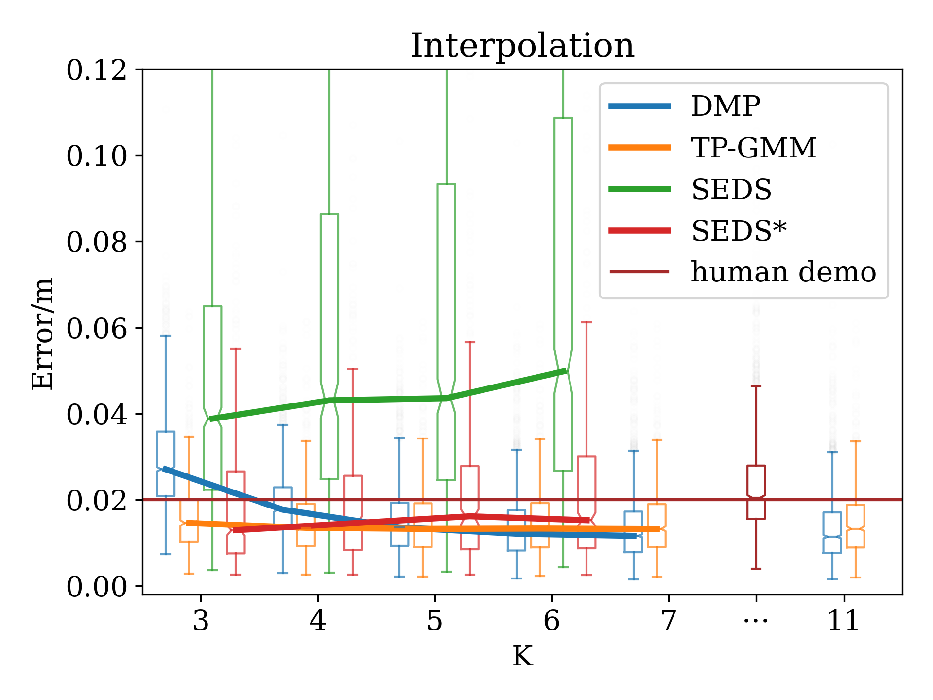
(a)

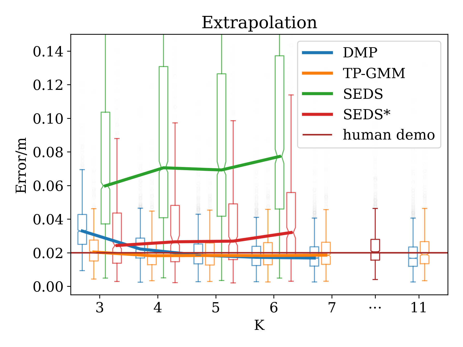
(b)

Figure 8: Comparison of movement encoding frameworks on the movement generalisation task when only few demonstration trajectories are available in case of interpolation (a) and extrapolation (b). Median error vs. number of kernels is shown for each model. Failed SEDS encodings are not included in this statistics (see Section III-A2). Note, there are no results for SEDS for $K>6$ because the encoding time for high $K$ values using the repeated optimization method (see Section II-D1) becomes impractically long. In case of human demo, error denotes the variance among human demonstrations whereas for models, error denotes deviation from human demonstration (see Section II-F3).

Errors for the extrapolation cases are consistently higher than for the interpolation cases.

As in the reconstruction case, the DMP model shows a big increase in accuracy for $K>3$.

The SEDS model performs the worst of the three models and has much wider error distributions as compared to the other two models.

In case of the relaxed time condition (SEDS*), the error is comparable to the other models for interpolation, but still higher for extrapolation as compared to DMP and TP-GMM.

One can also observe that the errors are not converging to zero if the number of kernels $K$ is increased, but saturate for larger $K$.

Considering the number of parameters, both SEDS and TP-GMM now use nearly the same number of parameters with $29K$ and $29K-1$, respectively. Because the average number of demonstrations is 6, the DMP averaging procedure to obtain generalised trajectory uses $18K$ parameters. This is still less than the other models, but significantly more (six times) than in reconstruction.

III-B2 Generalisation using many demonstration trajectories

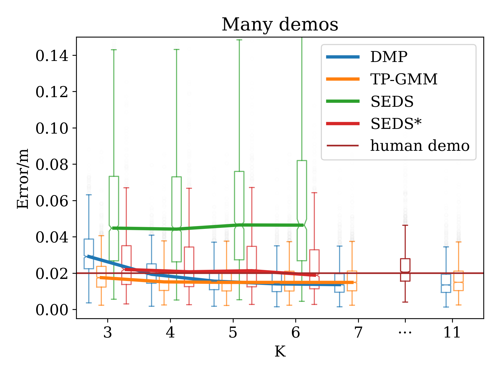
Figure 9: Comparison of movement encoding frameworks on the movement generalisation task when many demonstration trajectories are available. Median error vs. number of kernels is shown for each model. Please see the caption of Figure 8 for other relevant remarks on the SEDS model.

Results for the generalisation using many demonstration trajectories are show in Figure 9. This set of generalizations contains all possible target positions with all available demonstrations, as the difference between inter- and extrapolation is not well defined in this case. There is no qualitative change in the error curves as compared to the case of generalisation with few demonstrations. The absolute error is comparable to the interpolation case. The number of SEDS reconstructions with large error is smaller than with few demonstrations.

SEDS and TP-GMM still use the same number of parameters, since they encode everything into one model. Hence, the number of demonstrations has no effect on the number of parameters used. The DMP model, however, uses more, because the set of demonstrations used is now even bigger that before. Since there are 13 possible start-/end-points (see Figure 2), one of which is the target, there are 12 positions in the demonstration set. With the three repetitions of each action, the average demonstration set contains 36 moves (there might be extra/forgotten repetitions or exclusions as defined in II-F2). This yields $108K$ DMP parameters that are used in the averaging procedure to obtain a generalized trajectory.

III-B3 Behaviour and convergence of SEDS

TABLE II: Percentages of successful SEDS encodings. Optim. success is the percentage of cases where the optimization succeeds by the procedure defined in II-D1, regardless of the generalization quality. End-point conv. success is the percentage of cases where SEDS converge to the end-point under the relaxed time condition (SEDS*) given in Section II-F3. The last row contains the union over all $K$. The other two models have 100% optimization success rate and always converge to the end-point on time. TP-GMM however does not always hit the correct end point, which is discussed in Section III-C.

$K$	Interpolation		Extrapolation		Many demos
	Optim.	End-point	Optim.	End-point	Optim.	End-point
	success	conv. success	success	conv. success	success	conv. success
3	89%	58%	95%	44%	94%	51%
4	82%	54%	96%	42%	82%	54%
5	89%	61%	90%	39%	88%	55%
6	78%	49%	81%	35%	71%	46%
all	99.9%	88%	99.7%	73%	99.8%	80%

The SEDS model gives no guarantee for end-point convergence within the specified time in case of generalised trajectories that are not similar to the demonstrations it had been fitted to. However, the smoothness of its state space leads to the reasonable assumption that it can indeed generalize to different positions. There are many cases where the model takes much longer (see Figure 6(b)) or is faster (see Figure 6(e)) than the target trajectory. Figure 7 shows the generalization case presented in Figure 6(b) integrated for a longer time. This specific case does not fulfill the requirement of converging to the target on time, since it takes 1.28 s instead of the original 0.74 s, which is more than a 38% increase of the movement duration.

Table II summarizes the success rates of SEDS encodings for the optimization procedure (Optim. success) as defined in Section II-D1 and for the converge to the end-point under the relaxed time condition (End-point conv. success) as given in Section II-F3. We can see that in summary over all $K$ (last row of Table II), almost all demonstration trajectories can be encoded by the SEDS model, however, not all of those models represent generalized trajectories that converge to the target point even under the relaxed time condition. In general, the ratio of optimization success has a tendency to decrease with higher $K$, as optimizing more kernels is harder.

III-C Convergence to the end-point

Figure 10 shows the median deviation of the end-point of the generalized trajectory from the end-point of the target trajectory. Here, $K=6$ was used for all models.

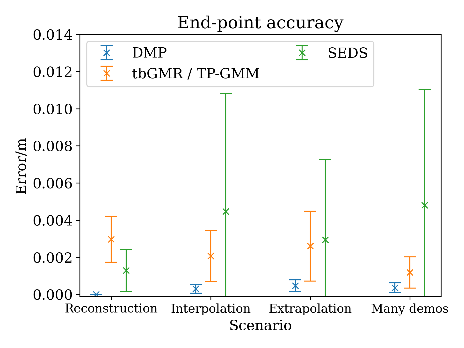
Figure 10: Comparison of movement encoding frameworks with respect to the end-point accuracy. Median error is shown for each model. The error bars denote median absolute deviation. Note that tbGMR was used in the reconstruction scenario, whereas TP-GMM was used in all other scenarios.

Most notably, the SEDS model performs much worse as compared to the other two models. This is due to the problem of the end-point convergence on-time as discussed in the previous Section III-B3, which leads to many of cases with an end-point error of 10 cm or more.

We also see that, as discussed above, the TP-GMM model does not converge to the exact end-point.

The median end-point error for DMPs is zero for the reconstruction case and always below half a millimeter for the generalization cases, which makes DMPs the best model with respect to the end-point convergence.

IV Discussion

IV-A Key Model Differences

The three models investigated in this study represent different approaches for encoding, reconstructing and generalization of movement trajectories. They all have different requirements and give different guarantees with respect to the solutions obtained by them. Here we briefly summarize the key differences of the models from a theoretical point of view.

DMP and SEDS are both based a dynamical system with an attractor. Therefore, the convergence of the trajectories from any start-point to the specified end-point is always guaranteed. DMP ensures convergence in a given time, while with SEDS the actual duration of a generalized movement depends on the obtained model.

For the TP-GMM model, the start- and end-points can only indirectly be set by defining new task parameters. Whether the model will reach these points or not is determined by the quality of the model fit achieved from demonstration data, however there is no guarantee that the generalised trajectory will start and end at the points specified by the task parameters. Furthermore, the lack of an intrinsic dynamical system means that an external controller is needed to generate control signals for perturbation recovery.

All the GMM based models contain cross correlations between the different dimensions represented by the off-diagonal entries of the covariance matrix, whereas DMPs have fully independent models for each dimension. While for GMM based models this turned out to be not beneficial for movement encoding, reconstruction, and generalisation, this might be beneficial for other tasks such as movement recognition.

In Table III we provide a summary for the numbers of free parameters in the different models as derived in the previous sections.

TABLE III: Number of free model parameters $n_{p}$ for 3D trajectories. The numbers $K$ and $N$ correspond to the number of kernels and the number of demonstrations, respectively.

	DMP	tbGMR	TP-GMM	SEDS
Reconstruction	$3K$	$15K-1$		$29K$
Generalization	$3NK$		$29K-1$	$29K$

Because the non DMP models use multivariate Gaussian kernels instead of 1D Gaussian kernels with fixed center and variance, they use significantly more parameters. The parameter number in the covariance matrices of the GMMs scales with $D^{2}$, while DMPs only scale with $D$. Note that the comparatively lower number of parameters in DMPs does not directly imply that they are a more efficient for trajectory encoding. While this might be true for simple reconstruction without generalization, the GMM based models also retain information about the variance in the demonstrations and cross correlations between dimensions, that DMPs do not encode at all.

IV-B Influence of Hyperparameters

For both DMP and tbGMR we conducted parameter searches to find optimal hyperparameters. For generalization with TP-GMM, it proved to be impossible to use the regularization for keeping trajectories smooth, while also maintaining good accuracy. Especially in the case of using few demonstrations, where regularization is needed to keep the models from overfitting to the few available demonstrations, high regularization leads to higher errors and the generalized trajectories miss the target end-points in most of the cases. Lowering the regularization reduces the error in the position profiles, however, it introduces oscillations in the velocity profiles.

The more kernels are used, the smaller the absolute value of the oscillations becomes, still the qualitative behaviour does not change. To test if this behaviour is specific to our dataset, we reproduced the reconstruction and generalization experiments as in [9] and looked at their velocity profiles. We found that also with their chosen regularization, the velocity profiles of their reconstructions and generalizations oscillate as observed in our case.

Since this undesired behaviour of the TP-GMM could not be fixed by means of the model itself, we lowered the regularization to reduce errors in position profiles, and solved the velocity oscillation problem by utilising a low-pass filter.

IV-C Influence of the Number of Demonstration Trajectories

The difference between generalizing with few or many demonstrations is significant. In case of many demonstrations, the TP-GMM model improves its end-point convergence by more than 50% as compared to the case with few demonstrations.

For SEDS, the number of encodings with high generalization error decreases with more demonstrations. Comparing Figures 8 and 9, we see that the third quartile of the error distributions when using many demonstrations is lower than for few demonstrations in most of the cases.

Furthermore, when looking at Table II, we see an additional dependence on nature of the presented demonstrations. The optimization success for individual $K$ values is higher for extrapolation than interpolation, indicating this case is easier. But, the generalization error for extrapolation is worse than for interpolation, (also see Figure 8(a) and Figure 8(b)), indicating it is harder. We suppose that encoding an extrapolation model as such is actually easier than encoding an interpolation model, because in case of extrapolations the demonstrations are closer together than for interpolations. However, obtaining an attractor landscape for accurate generalizations outside demonstrations is less probable for extrapolation than obtaining an attractor landscape within demonstrations for interpolation, raising the number of extrapolation cases that do not meet the relaxed time convergence criteria.

For DMPs, the usage of many demonstrations as compared to few demonstrations did not change the results significantly.

IV-D Choosing Encoding and Optimisation for a Model

The TP-GMM approach is agnostic of the underlying GMM used. The distributions and task parameters chosen in Section II-C2 can be chosen differently, to represent the encoded trajectories in a different way. The paper on TP-GMMs by Calinon and co-workers [9] presents a lot more possibilities to encode and generalize trajectories with TP-GMMs. Future work could test more of these encoding variants to see if they lead to easier hyperparameter tuning for smooth trajectories without losing good end-point convergence.

To improve the optimization convergence of the SEDS model, a different solver could be used. The paper on SEDS [8] mentions a custom written solver that has “several advantages over general purpose solvers” (see Section V. in the paper), that was unfortunately not published with the rest of the code, so we used the general purpose solver. Also, there is no guarantee that a better local optimum of the loss function would yield a better generalization.

Our DMP optimization algorithm could also be improved. The implications of the very simple $\delta$-rule with its simple loss function can be clearly seen in the reconstructions with only few parameters (for example Figure 4(a) and 4(b)). For $K=3$ the error is 0 at three places, the centers of the Gaussian kernels that matter for the $\delta$-learning. To improve the encoding quality, theoretically, any other more sophisticated supervised learning rule could be used, for example ones that would optimize the encoding based on the whole trajectory or adjust the centers and variances of the Gaussian kernels [26, 29, 30]. Using variable position kernels could improve the DMP results, but this would prevent the averaging of weight vectors to obtain generalized trajectories and, therefore, some other generalisation mechanism would be needed instead.

IV-E Encoding and Inference Time

We will only make relative statements about the inference and encoding times of our models, since it is always possible to take more or less potent hardware with which different runt-times will be obtained.

The inference times of all three models are significantly faster then the respective encoding times. GMM based models are slower than DMPs, but still fast enough for online motion generation for robotic applications.

The differences of encoding times are more prominent. DMPs, as the simplest model without matrix multiplications and with a simple loss function that is only a difference between values, are significantly faster than the GMM based models. While the tbGMR approach remains on the order of seconds, a run-time of the SEDS optimization can take on the order of a minute.

IV-F Other Considerations

Given that the DMP model achieves better results than the GMM based models for generalization of simple manipulation actions, it does not mean that DMPs will be also beneficial for more complex actions or different tasks.

In more complex cases, DMPs would probably have to be augmented with via points [5] or be represented as chains of joined simpler actions [25], because our simple method of averaging based on goal positions would not be applicable anymore. For TP-GMMs, it would be necessary to work with more reference frames. Because of its global state space and smoothing constraint, it does not seem that SEDS would be able to generalize well over more complex actions.

One property of the GMM based encodings, the cross correlation between dimensions, was not assessed in this work. More research is needed to investigate the benefit of these off-diagonal elements of covariance matrices for other tasks, e.g., movement recognition based on GMM or DMP encoding parameters.

V Conclusions

In this work we compared three of the most widely used encoding frameworks in robotics: dynamic motion primitives (DMPs), and two variants of Gaussian mixture based models, time based Gaussian mixture model (tbGMM) and trajectory encoding and generation using stable estimator of dynamical systems (SEDS).

We showed that the encoding of single trajectories from our dataset of human manipulation actions for reconstruction is possible for all models with an accuracy comparable to our tracking error estimate, given that enough kernels are used. However, the SEDS model does not always converge to the demonstration just by increasing the number of kernels.

The GMM based models with their multidimensional Gaussian kernels use significantly more parameters than DMPs, but do not achieve better results.

Tuning the hyperparameters of the system is easiest for DMPs. When using the tbGMR approach, care has to be taken to not under-regularize the model. While low regularization improves the reconstruction error of position profiles, it also introduces oscillations in velocity profiles.

Generalization from demonstrations in our dataset to new targets is possible with all analysed models, but they all have different strengths and weaknesses. The DMP model is easiest to operate, because it requires no additional hyperparameter considerations, as it re-uses existing encodings, always converges and produces generalizations comparable to the human inter-demonstration variation in every condition. The TP-GMM model achieves comparable results in terms of position profiles of the generalised trajectories, but fails to reach the target end-point point precisely. The SEDS model was not primarily developed to perform this kind of generalization, so it performs worse as compared to other two models, however, generalization is also possible to some extent. However, the convergence problems with the nonlinear optimization, the inferior generalization quality and the long encoding times makes SEDS impractical for many situations.

In conclusion, we found that for our large dataset of human manipulation actions the DMP model is the most efficient with respect to the hyperparameter tuning, encoding and generalisation accuracy.

VI Research Data

The dataset used in this work is published on Zenodo: https://doi.org/10.5281/zenodo.7351664.

Appendix A DMP Model Variations

A-A DMP Model Simplification

In this work we simplified the DMP formulation presented in [25] by removing the function $v$ from the computation of the function $f$. The function $v$ is a sigmoid that drops from 1 to 0 in a very short time around the end-time $T$ of a trajectory ($v(t)=0.5$ at $t=T$). This function was specifically designed for joining of movement trajectories which allows blending of DMP kernels at the joining point without affecting the influence of kernels at the joining point. If no joining is performed (or at the end of the joined motion), the function $v$ ensures that the trajectory converges to the goal point regardless of the shape of $f$ in time $t=T+\delta t$ (where $\delta t<<T$).

To make sure this modification does not affect the performance of the DMP formulation presented in [25], we computed all DMP encodings with the sigmoid function as well. Figure 11 compares the reconstruction accuracy between the models with and without $v$, exactly as in Section III-A1.

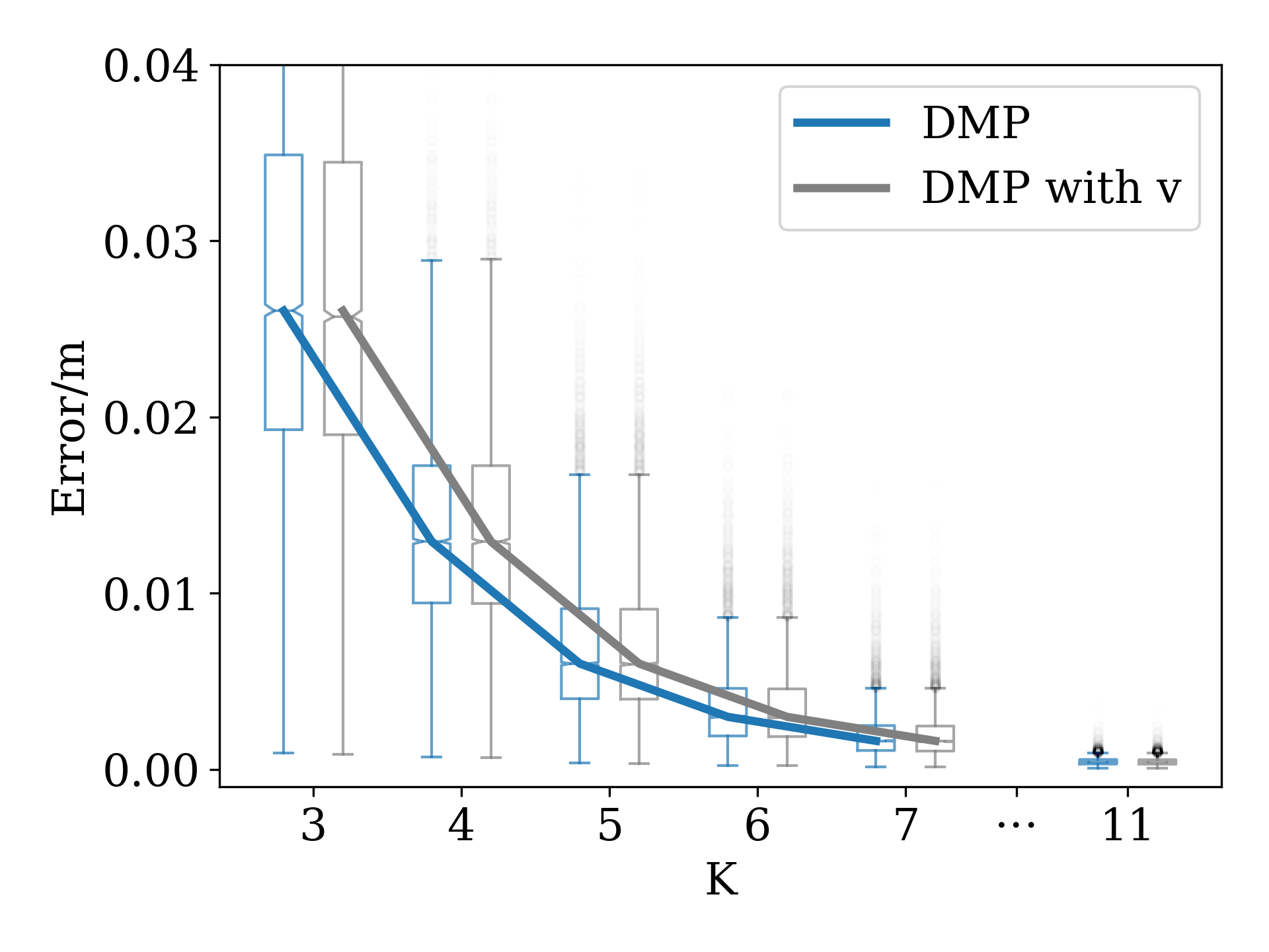
Figure 11: Comparison of DMP framework with and without $v$ on the movement reconstruction task.

There is no significant difference to the DMP variant without $v$. Since all generalizations are done using the encodings of the single trajectories, leaving out the sigmoid will have the same (no) effect on generalizations as well.

A-B DMP Generalization Variations

In addition to the DMP generalization method presented in Section II-B2, here we also include two other approaches, namely, generalization by changing end-point, and generalisation by using weighted averaging without constraints.

A-B1 Generalization by changing end-point

The simplest way to generalize a DMP to a new situation is to just change the goal point $g$ and use the weights without any changes. Instead of averaging the available demonstrations, we select the closest trajectory with respect to the generalization target and change its goal point to the new end-point.

A-B2 Generalisation using weighted distance average

Instead of computing averaging weights based on goals with constraints as explained in Section II-B2, one can also think of a simpler way to determine averaging weights. Another way to weigh the contribution of demonstrations is just by distance to the generalization target. For this, we also translate all the trajectories to a common reference frame, but instead of obtaining the weights from expressing the new goal as a linear combination of the demonstration goals, we just weigh the trajectories by the distance $d_{i}$ of their goal to the new target goal. We want close trajectories to have more influence than far away ones, so we take the inverse of $d_{i}$ and obtain the weights $\alpha_{i}$ as

$$x_{i}=1/d_{i},$$ (24)

$$\alpha_{i}=\frac{x_{i}}{\sum\limits_{i}x_{i}}.$$ (25)

The second equation normalizes the weights $\alpha_{i}$ such that $\sum\limits_{i}\alpha_{i}=1$.

A-B3 Comparison results

We compared the generalization strategies on both the few and many demonstration tasks as defined in Section II-F2.

Figure 12 shows the results for the generalization error evaluated like in Section III-B1.

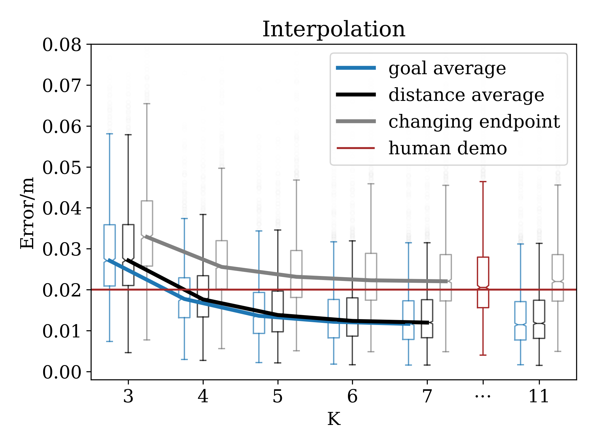
(a)

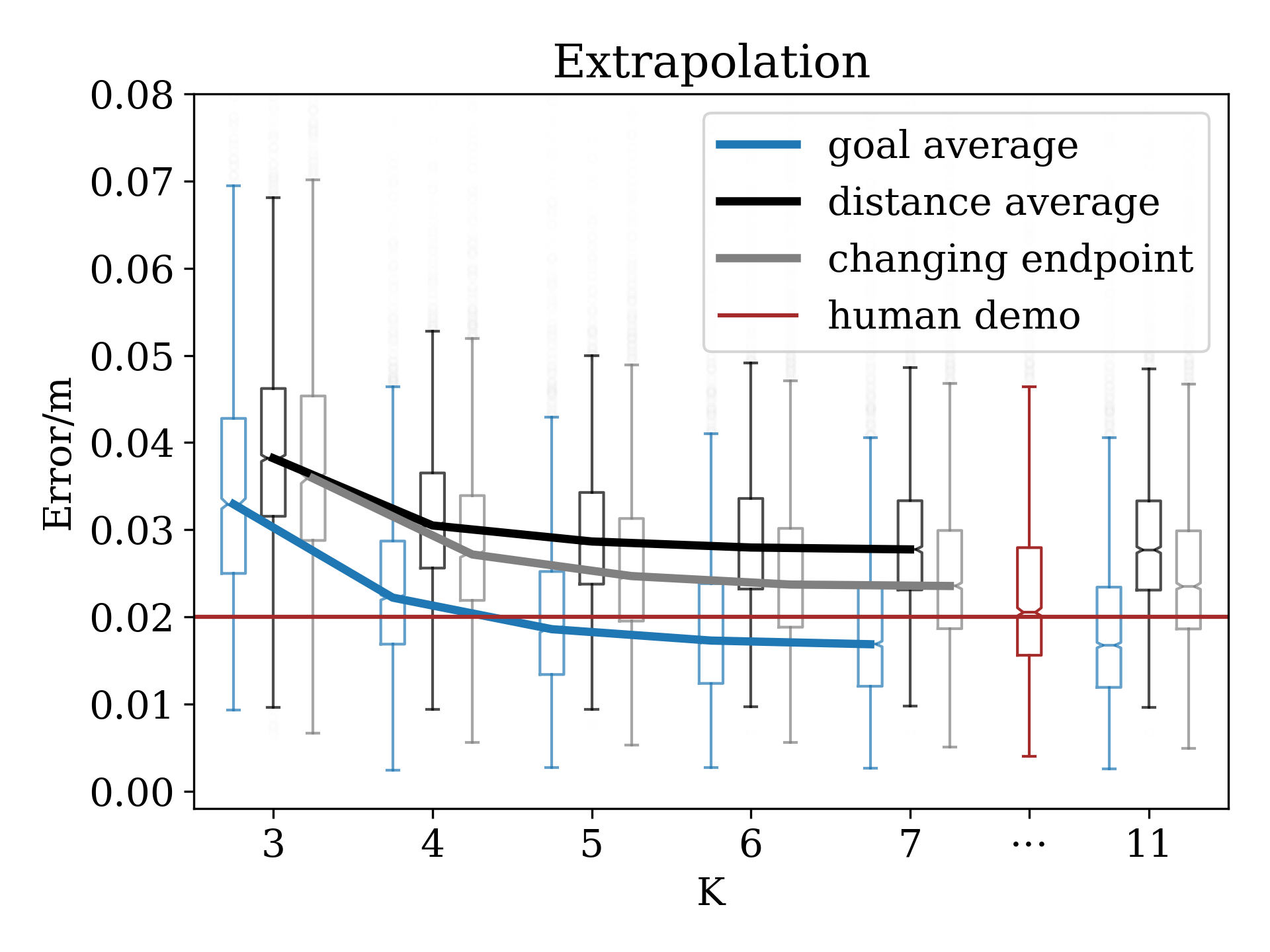
(b)

Figure 12: Comparison of movement encoding frameworks on the movement generalisation task when only few demonstration trajectories are available in case of interpolation (a) and extrapolation (b). Median error vs. number of kernels is shown for each model. In case of human demo, error denotes the variance among human demonstrations whereas for models, error denotes deviation from human demonstration (see Section II-F3).

The general trend of extrapolation errors being higher than interpolation errors is visible again. For interpolation, goal and distance averaging perform the same, because our demonstration scenario of two bundles of demonstrations to either side of the generalization target makes them choose the same weights. In extrapolation, there is a difference between the two, as pure distance averaging has no means of accounting for the spacial distribution of demonstrations. So it produces DMP weights that wold be suitable for a point between the demonstrations, but closer to the ones near the generalization target. The method is effectively still doing an interpolation, but to the wrong point. This results in errors even worse than simple end-point shifting. Generalisation by changing the end-point performs worse than the inter human variance in all situations. Additionally, there is less difference between interpolation and extrapolation than in the averaging cases. This could be explained by the fact that selecting the closest trajectory neglects the difference between the interpolation and extrapolation scenarios. There is always only one trajectory, so compared to averaging the spatial arrangement of the other available trajectories does not matter, leaving less difference between the two scenarios.

Figure 13 shows the results for the generalization error evaluated like in Section III-B2.

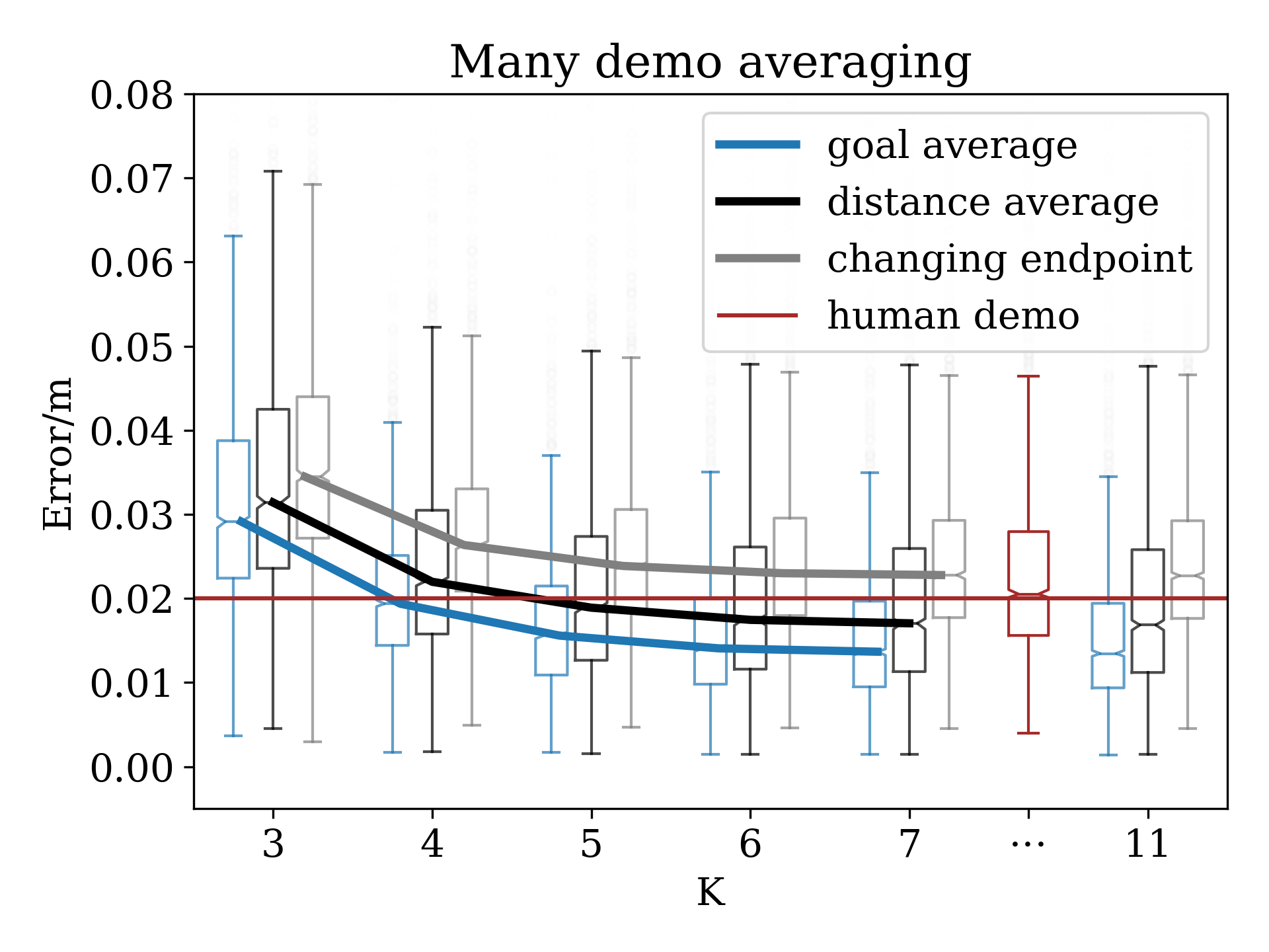
Figure 13: Comparison of movement encoding frameworks on the movement generalisation task when many demonstration trajecto- ries are available. Median error vs. number of kernels is shown for each model.

Again, goal point averaging performs the best of the three. The simplest method of changing the end point performs worse. Relative to the inter human human variance, both averaging methods get lower errors at high enough $K$, whereas the end-point changing stays above.

In conclusion, there is more accuracy gained by using a more complex method for obtaining new DMP weights, especially choosing an averaging approach over simple end-point changing. On the other hand, not using averaging does not cause the model to completely fail, so the choice of method depends on demonstration availability and deviation tolerance.

Appendix B Hyperparameter Tuning

All the considered models contain hyperparameters. Choosing them optimally improves their performance. To find the optimal hyperparameters for our models, we conducted parameter searches over sensible parameter regions on a limited set of 250 randomly chosen actions for each individual number of kernels.

B-A DMP

To find the optimal $\kappa$, which determines the kernel variance $\sigma$ via Equation (5), we considered $\kappa$ between 0.6 and 1.2 in steps of 0.1. $\kappa=0.6$ corresponds to relatively narrow Gaussian kernels, where the $1\sigma$-intervals of kernels don’t overlap at all. With $\kappa=1.2$, the kernels are much wider such that their $1\sigma$-intervals overlap. The optimal $\kappa$ for our data is 0.7 for $K=[3\dots 10]$ and 1.1 for $K>10$.

B-B tbGMR

Choosing the regularization parameter $\epsilon$ for the tbGMR models is more complicated than in the DMP case. We conducted a parameter search within the range $[0.0110^{-7}]$. This is from the same order of magnitude as the data down to very little regularization that is only good for numerical stability. While the parameter scan clearly showed that it is best to use as little regularization as possible to achieve lowest reconstruction error, the shape of those trajectories was problematic. Different from human demonstrations, those tbGMR reconstructions looked like a piece-wise linear approximation and the velocity profile was qualitatively completely different, and contained oscillations. Therefore, we decided to not use the low regularization for the lowest reconstruction error, because we are comparing the frameworks on human actions and those trajectories were qualitatively completely different.

We estimated the necessary regularization to keep the model’s reconstructions from becoming to different from human demonstrations using two other metrics than only reconstruction error. We observed that there were as many oscillations in the velocity profile as kernels in the model, so we compared the corresponding frequency in the FFT of the velocity profile with the fundamental frequency of the motion. We considered a trajectory smooth enough if the oscillations caused by the kernels were lower than 20 % of the base frequency.

We also checked how far the end-points of the reconstructions are away for the end-points of human demonstrations. We considered 5 mm, our estimated error from the trajectory tracking, as the maximum acceptable value. We then selected the highest possible hyperparameters with less than 5 mm median end-point error that still remained under our oscillation threshold.

For $K=3$ it was not possible to fulfill both requirements at once, since the end-points were missed by more than 5 mm regardless of regularization. Therefore, we chose to allow more oscillations in this case and used the regularization for which the end-point error was below 5 mm.

Using the hyperparameters obtained by means of these two additional measures yields higher reconstruction errors, but the obtained trajectories are smoother, and are more similar to human demonstrations.

References

- [1] B. Siciliano, L. Sciavicco, L. Villani, and G. Oriolo. Robotics: Modelling, planning and control. Springer Publishing Company, 2009.
- [2] Aude Billard, Sylvain Calinon, Rüdiger Dillmann, and Stefan Schaal. Robot Programming by Demonstration. In Bruno Siciliano and Oussama Khatib, editors, Springer Handbook of Robotics, pages 1371–1394. Springer Berlin Heidelberg, Berlin, Heidelberg, 2008.
- [3] Harish Ravichandar, Athanasios S. Polydoros, Sonia Chernova, and Aude Billard. Recent Advances in Robot Learning from Demonstration. Annual Review of Control, Robotics, and Autonomous Systems, 3(1):297–330, May 2020.
- [4] Auke J. Ijspeert, Jun Nakanishi, Heiko Hoffmann, Peter Pastor, and Stefan Schaal. Dynamical Movement Primitives: Learning Attractor Models for Motor Behaviors. Neural Computation, 25(2):328–373, February 2013.
- [5] You Zhou, Jianfeng Gao, and Tamim Asfour. Learning Via-Point Movement Primitives with Inter- and Extrapolation Capabilities. In 2019 IEEE/RSJ International Conference on Intelligent Robots and Systems (IROS), pages 4301–4308, Macau, China, November 2019. IEEE.
- [6] Sebastian Herzog, Florentin Wörgötter, and Tomas Kulvicius. Generation of movements with boundary conditions based on optimal control theory. Robotics and Autonomous Systems, 94:1–11, August 2017.
- [7] Seyed M. Khansari-Zadeh and Aude Billard. BM: An iterative algorithm to learn stable non-linear dynamical systems with Gaussian mixture models. In 2010 IEEE International Conference on Robotics and Automation, pages 2381–2388, Anchorage, AK, May 2010. IEEE.
- [8] Seyed M. Khansari-Zadeh and Aude Billard. Learning Stable Nonlinear Dynamical Systems With Gaussian Mixture Models. IEEE Transactions on Robotics, 27(5):943–957, October 2011.
- [9] Sylvain Calinon. A tutorial on task-parameterized movement learning and retrieval. Intelligent Service Robotics, 9(1):1–29, January 2016.
- [10] You Zhou, Jianfeng Gao, and Tamim Asfour. Movement primitive learning and generalization: Using mixture density networks. IEEE Robotics & Automation Magazine, 27(2):22–32, 2020.
- [11] Alexandros Paraschos, Christian Daniel, Jan Peters, and Gerhard Neumann. Probabilistic Movement Primitives. Advances in Neural Information Processing Systems (NIPS), page 9, January 2013.
- [12] Matteo Saveriano, Fares J. Abu-Dakka, Aljaz Kramberger, and Luka Peternel. Dynamic movement primitives in robotics: A tutorial survey. CoRR, abs/2102.03861, 2021.
- [13] Sylvain Calinon, Tohid Alizadeh, and Caldwell G. Darwin. On improving the extrapolation capability of task-parameterized movement models. In 2013 IEEE/RSJ International Conference on Intelligent Robots and Systems, pages 610–616, November 2013. Journal Abbreviation: 2013 IEEE/RSJ International Conference on Intelligent Robots and Systems.
- [14] A. Lemme, Y. Meirovitch, M. Khansari-Zadeh, T. Flash, A. Billard, and J. J. Steil. Open-source benchmarking for learned reaching motion generation in robotics. Paladyn, Journal of Behavioral Robotics, 6(1), March 2015. Publisher: De Gruyter Open Access.
- [15] Sylvain Calinon, Florent Guenter, and Aude Billard. On Learning, Representing, and Generalizing a Task in a Humanoid Robot. IEEE Transactions on Systems, Man and Cybernetics, Part B (Cybernetics), 37(2):286–298, April 2007.
- [16] Pham N. Hung and Takashi Yoshimi. An approach to learn hand movements for robot actions from human demonstrations. In 2016 IEEE/SICE International Symposium on System Integration (SII), pages 711–716, December 2016.
- [17] Ales Ude, Andrej Gams, Tamim Asfour, and Jun Morimoto. Task-Specific Generalization of Discrete and Periodic Dynamic Movement Primitives. Robotics, IEEE Transactions on, 26:800–815, November 2010.
- [18] Florentin Wörgötter, Eren Erdal Aksoy, Norbert Krüger, Justus Piater, Ales Ude, and Minija Tamosiunaite. A Simple Ontology of Manipulation Actions Based on Hand-Object Relations. IEEE Transactions on Autonomous Mental Development, 5(2):117–134, June 2013.
- [19] Alexander Mathis, Pranav Mamidanna, Kevin M. Cury, Taiga Abe, Venkatesh N. Murthy, Mackenzie Weygandt Mathis, and Matthias Bethge. DeepLabCut: markerless pose estimation of user-defined body parts with deep learning. Nature Neuroscience, 21(9):1281–1289, September 2018. Number: 9 Publisher: Nature Publishing Group.
- [20] Tanmay Nath, Alexander Mathis, An Chi Chen, Amir Patel, Matthias Bethge, and Mackenzie Weygandt Mathis. Using DeepLabCut for 3D markerless pose estimation across species and behaviors. Nature Protocols, 14(7):2152–2176, July 2019. Number: 7 Publisher: Nature Publishing Group.
- [21] Alexander Mathis and Mackenzie Mathis. DeepLabCut/DeepLabCut, 2018.
- [22] Pierre Karashchuk, Katie L. Rupp, Evyn S. Dickinson, Elischa Sanders, Eiman Azim, Bingni W. Brunton, and John C. Tuthill. Anipose: a toolkit for robust markerless 3D pose estimation. bioRxiv, page 2020.05.26.117325, May 2020. Publisher: Cold Spring Harbor Laboratory Section: New Results.
- [23] Pierre Karashchuk and Katie L. Rupp. lambdaloop/anipose, 2019.
- [24] Stefan Schaal, Peyman Mohajerian, and Auke Ijspeert. Dynamics systems vs. optimal control — a unifying view. In Progress in Brain Research, volume 165, pages 425–445. Elsevier, 2007.
- [25] Tomas Kulvicius, KeJun Ning, Minija Tamosiunaite, and Florentin Worgötter. Joining Movement Sequences: Modified Dynamic Movement Primitives for Robotics Applications Exemplified on Handwriting. IEEE Transactions on Robotics, 28(1):145–157, February 2012.
- [26] Auke Jan Ijspeert, Jun Nakanishi, and Stefan Schaal. Movement imitation with nonlinear dynamical systems in humanoid robots. In Proceedings 2002 IEEE International Conference on Robotics and Automation (Cat. No. 02CH37292), volume 2, pages 1398–1403. IEEE, 2002.
- [27] Simon Haykin. Neural Networks: A Comprehensive Foundation. N.J.: Prentice Hall, Englewood Cliffs,, 1999.
- [28] Arthur P. Dempster, Nan M. Laird, and Donald B. Rubin. Maximum Likelihood from Incomplete Data Via the EM Algorithm. Journal of the Royal Statistical Society: Series B (Methodological), 39(1):1–22, September 1977.
- [29] Stefan Schaal and Christopher G Atkeson. Constructive incremental learning from only local information. Neural computation, 10(8):2047–2084, 1998.
- [30] Sethu Vijayakumar and Stefan Schaal. Locally weighted projection regression: An o (n) algorithm for incremental real time learning in high dimensional space. In Proceedings of the seventeenth international conference on machine learning (ICML 2000), volume 1, pages 288–293. Morgan Kaufmann, 2000.