Mitigating Data Sparsity for Short Text Topic Modeling
by Topic-Semantic Contrastive Learning

Abstract

To overcome the data sparsity issue in short text topic modeling, existing methods commonly rely on data augmentation or the data characteristic of short texts to introduce more word co-occurrence information. However, most of them do not make full use of the augmented data or the data characteristic: they insufficiently learn the relations among samples in data, leading to dissimilar topic distributions of semantically similar text pairs. To better address data sparsity, in this paper we propose a novel short text topic modeling framework, Topic-Semantic Contrastive Topic Model (TSCTM). To sufficiently model the relations among samples, we employ a new contrastive learning method with efficient positive and negative sampling strategies based on topic semantics. This contrastive learning method refines the representations, enriches the learning signals, and thus mitigates the sparsity issue. Extensive experimental results show that our TSCTM outperforms state-of-the-art baselines regardless of the data augmentation availability, producing high-quality topics and topic distributions.

1 Introduction

Topic models aim to discover the latent topics of a document collection and infer the topic distribution of each document in an unsupervised fashion Blei et al. (2003). Due to the effectiveness and interpretability, topic models have been popular for decades with various downstream applications Ma et al. (2012); Mehrotra et al. (2013); Boyd-Graber et al. (2017). However, despite the success on long texts, current topic models generally cannot handle well short texts, such as tweets, headlines, and comments Yan et al. (2013). The reason lies in that topic models rely on word co-occurrence information to infer latent topics, but such information is extremely scarce in short texts Qiang et al. (2020). This issue, referred to as data sparsity, can hinder state-of-the-art topic models from discovering high-quality topics and thus has attracted much attention.

$\boldsymbol{\mathbf{x}}^{(i)}$	april fool’s jokes range from hilarious to disastrous
$\boldsymbol{\mathbf{x}}^{(i)}_{+}$	april sucker ’ s laugh range from hilarious to disastrous
$\boldsymbol{\mathbf{x}}^{(\ell)}$	april fools’ joke goes wrong for cleveland woman
$\boldsymbol{\mathbf{x}}^{(j)}$	should airlines create separate sections for kids, larger fliers?

(a) Examples of short texts.

	$\boldsymbol{\mathbf{x}}^{(i)}_{+}$	$\boldsymbol{\mathbf{x}}^{(\ell)}$	$\boldsymbol{\mathbf{x}}^{(j)}$
$\boldsymbol{\mathbf{x}}^{(i)}$	0.479	0.377	0.922

(b) NQTM

	$\boldsymbol{\mathbf{x}}^{(i)}_{+}$	$\boldsymbol{\mathbf{x}}^{(\ell)}$	$\boldsymbol{\mathbf{x}}^{(j)}$
$\boldsymbol{\mathbf{x}}^{(i)}$	0.995	0.984	0.078

(c) TSCTM

Figure 1: (a): Examples of short texts from TagMyNews title dataset. Text $\boldsymbol{\mathbf{x}}^{(i)}_{+}$ is an augmented view of $\boldsymbol{\mathbf{x}}^{(i)}$, and $\boldsymbol{\mathbf{x}}^{(i)}$ and $\boldsymbol{\mathbf{x}}^{(\ell)}$ are relevant while $\boldsymbol{\mathbf{x}}^{(i)}$ and $\boldsymbol{\mathbf{x}}^{(j)}$ are irrelevant. (b, c): Heat map of cosine similarity between learned topic distributions. The similarities of our TSCTM are more reasonable than NQTM.

To overcome the data sparsity issue, traditional wisdom can be mainly categorized into two lines: (i) Augment datasets with more short texts containing similar semantics Phan et al. (2008); Jin et al. (2011); Chen and Kao (2015). This way can feed extra word co-occurrence information to topic models. (ii) Due to the limited context, many short texts in the same collection, such as tweets from Twitter, tend to be relevant, sharing similar topic semantics Qiang et al. (2020); to leverage this data characteristic, models such as DMM Yin and Wang (2014); Li et al. (2016) and state-of-the-art NQTM Wu et al. (2020b) learn similar topic distributions from relevant samples. These two lines of thought have been shown to achieve good performance and mitigate data sparsity to some extent.

However, existing short text topic models neither make full use of the augmented data nor the crucial data characteristic. To begin with, an augmented text is expected to have a similar topic distribution as the original text since they share similar topic semantics, but existing approaches tend to overlook this important relation between samples. As shown in Figure 1(b), text $\boldsymbol{\mathbf{x}}^{(i)}$ and its augmented view $\boldsymbol{\mathbf{x}}^{(i)}_{+}$ have similar topic semantics, but their topic distributions inferred by NQTM are far from similar. Moreover, guided by the aforementioned data characteristic, state-of-the-art methods like NQTM attempt to learn similar topic distributions for relevant samples, yet they could inappropriately do so. Figure 1(b) shows that text $\boldsymbol{\mathbf{x}}^{(i)}$ and $\boldsymbol{\mathbf{x}}^{(\ell)}$ are relevant, but their learned topic distributions are dissimilar; $\boldsymbol{\mathbf{x}}^{(i)}$ and $\boldsymbol{\mathbf{x}}^{(j)}$ are irrelevant, but theirs are similar. In a word, current approaches insufficiently model the relations among samples in data, which hinders fully addressing the data sparsity issue.

To better mitigate data sparsity, we in this paper propose Topic-Semantic Contrastive Topic Model (TSCTM), a novel short text topic modeling framework that unifies both cases with and without data augmentation. To be specific, TSCTM makes full use of relations among samples with a novel topic-semantic contrastive learning method. In the case without data augmentation, TSCTM effectively samples positive and negative text pairs based on topic semantics. In the case with data augmentation, TSCTM also smoothly incorporates the relations between augmented and original samples, enabling better utilization of data augmentation. Through the novel contrastive learning method, TSCTM sufficiently models the relations among samples, which enriches the learning signals, refines the learning of representations, and thus mitigates the data sparsity issue (see Figure 1(c) for an illustration). We summarized the main contributions of this paper as follows:

• We follow a contrastive learning perspective and propose a novel contrastive learning method with efficient positive and negative pairs sampling strategies to address the data sparsity issue in short text topic modeling.

• We propose a novel short text topic modeling framework, Topic-Semantic Contrastive Topic Model (TSCTM), which is the first such framework that concerns both cases with and without data augmentation.

• We validate our method with extensive experiments where TSCTM effectively mitigates data sparsity and consistently surpasses state-of-the-art baselines, producing high-quality topics and topic distributions.

2 Related Work

Topic Modeling

Based on classic long text topic models Hofmann (1999); Blei et al. (2003); Lee et al. (2020), various probabilistic topic models for short texts have been proposed Yan et al. (2013); Yin and Wang (2014); Li et al. (2016); Wu and Li (2019). They use Gibbs Sampling Griffiths and Steyvers (2004) or Variational Inference Blei et al. (2017) to infer model parameters. Later, due to the effectiveness and brevity of Variational AutoEncoder (VAE, Kingma and Welling, 2014; Rezende et al., 2014), many neural topic models have been introduced Miao et al. (2016, 2017); Srivastava and Sutton (2017); Card et al. (2018); Nan et al. (2019); Dieng et al. (2020); Li et al. (2021); Wu et al. (2020a, b, 2021); Wang et al. (2021). Among those methods, the most related one to this paper is NQTM Wu et al. (2020b). Although NQTM also uses vector quantization to aggregate the short texts with similar topics, however, we note that our method differs significantly in that: (i) Our TSCTM framework uses the novel topic-semantic contrastive learning method that fully considers the relations among samples with effective positive and negative sampling strategies, while NQTM only considers the relations between samples with similar semantics. (ii) Our TSCTM framework can adapt to the case with data augmentation by sufficiently modeling the relations brought by augmented samples, achieving higher performance gains, while NQTM cannot fully incorporate such relations.

Contrastive Learning

The idea of contrastive learning is to measure the similarity relations of sample pairs in a representation space Hadsell et al. (2006); Oh Song et al. (2016); Hjelm et al. (2018); Van den Oord et al. (2018); Frosst et al. (2019); Wang et al. (2019); He et al. (2020); Wang and Isola (2020). It has been widely explored in the visual field, such as image classification Chen et al. (2020); Khosla et al. (2020), objective detection Xie et al. (2021), and image segmentation Zhao et al. (2021). For text data, some studies use contrastive loss Gao et al. (2021); Nguyen and Luu (2021) by sampling salient words from texts to build positive samples, but they could be inappropriate for short text topic modeling due to the limited context of short texts (shown in Sec. 5.1). In contrast, our new framework can discover effective samples for learning contrastively based on the topic semantics and can smoothly adapt to the case with augmentations, both of which better fit the short text modeling context.

3 Methodology

In this section, we first review the background of topic modeling. Then we introduce topic-semantic contrastive learning, a novel approach for short text topic modeling. Finally, we put this contrastive learning into the topic modeling context and propose our Topic-Semantic Contrastive Topic Model.

3.1 Notations and Problem Setting

Our notations and problem setting of topic modeling follow LDA Blei et al. (2003). Consider a collection of $N$ documents $\{\boldsymbol{\mathbf{x}}^{(1)},\dots,\boldsymbol{\mathbf{x}}^{(N)}\}$ with $V$ unique words, i.e., vocabulary size. We require to discover $K$ topics from the collection. Each topic is interpreted as its relevant words and defined as a distribution over all words (topic-word distribution): $\boldsymbol{\mathbf{\beta}}_{k}\in\mathbb{R}^{V}$. Then, $\boldsymbol{\mathbf{\beta}}\!=\!(\boldsymbol{\mathbf{\beta}}_{1},\dots,\boldsymbol{\mathbf{\beta}}_{K})\!\in\!\mathbb{R}^{V\times K}$ is the topic-word distribution matrix. A topic model also infers what topics a document contains, i.e., the topic distribution of a document, denoted as $\boldsymbol{\mathbf{\theta}}\in\Delta_{K}$. 

3.2 Topic-Semantic Contrastive Learning

The core difference between our TSCTM and a conventional topic model lies in that we employ the novel topic-semantic contrastive learning method to model the relations among samples. As such, the learning signals are enriched through sufficiently modeling the relations among texts to address the data sparsity issue. Figure 2 illustrates our topic-semantic contrastive learning method.

3.2.1 Encoding Short Texts

To employ our topic-semantic contrastive learning, the first step is to encode short text inputs into a semantic space and obtain the corresponding representations and topic distributions. Specifically, we employ an encoder neural network $f_{\Theta}$ with parameter $\Theta$ to encode short text $\boldsymbol{\mathbf{x}}^{(i)}$ and get its representation $\boldsymbol{\mathbf{h}}^{(i)}=f_{\Theta}(\boldsymbol{\mathbf{x}}^{(i)})$. The topic distribution of $\boldsymbol{\mathbf{x}}^{(i)}$ is denoted as $\boldsymbol{\mathbf{\theta}}^{(i)}$ and is computed by normalizing $\boldsymbol{\mathbf{h}}^{(i)}$ into a probability simplex with a softmax function as $\boldsymbol{\mathbf{\theta}}^{(i)}=\mathrm{softmax}(\boldsymbol{\mathbf{h}}^{(i)})$. Note that we train topic distribution $\boldsymbol{\mathbf{\theta}}^{(i)}$ with a topic modeling objective, which will be introduced later.

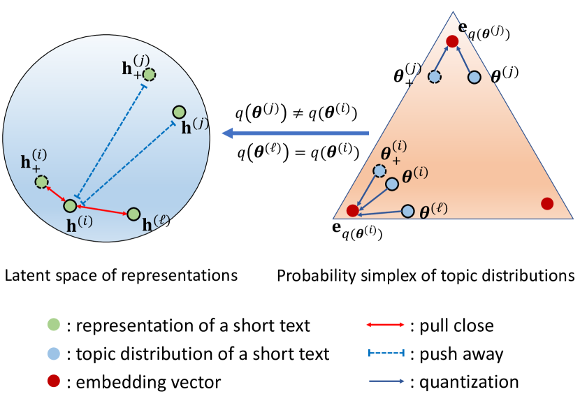
Figure 2: Illustration of the proposed topic-semantic contrastive learning. It refines the learning of representations through modeling the relations of samples according to their topic semantics (only solid line circles exist when without data augmentation).

3.2.2 Positive Pairs for Contrastive Learning

To utilize the vital characteristic of short texts (many short texts in a collection like Twitter tend to share similar topics due to the limited context), we propose to find those semantically similar texts and model them as positive pairs to each other for contrastive learning. Therefore, we can employ a contrastive learning objective to align those semantically similar texts in terms of representations and thus topic distributions.

However, it is non-trivial to find those semantically similar texts as positive pairs. Some previous methods like CLNTM Nguyen and Luu (2021) samples salient words to build positive pairs for long texts, but this way does not fit short texts well due to the extremely limited context (shown in Sec. 5.1). Differently, DMM Yin and Wang (2014); Li et al. (2016) follows a clustering process to aggregate short texts with similar topics, but lacks the flexibility of model design as it requires model-specific derivations for parameter inference. As such, we propose to employ vector quantization van den Oord and Vinyals (2017) to find positive pairs for short texts.

Specifically, as shown in Figure 2, we first quantize topic distribution $\boldsymbol{\mathbf{\theta}}^{(i)}$ to the closest embedding vector, and its quantized topic distribution $\boldsymbol{\mathbf{\theta}}_{q}^{(i)}$ is computed as:

$$\boldsymbol{\mathbf{\theta}}_{q}^{(i)} =\boldsymbol{\mathbf{e}}_{q(\boldsymbol{\mathbf{\theta}}^{(i)})}$$ (1)

$$q(\boldsymbol{\mathbf{\theta}}^{(i)}) =\mathrm{argmin}_{k}\|\boldsymbol{\mathbf{\theta}}^{(i)}-\boldsymbol{\mathbf{e}}_{k}\|_{2}.$$ (2)

Here, $(\boldsymbol{\mathbf{e}}_{1},\boldsymbol{\mathbf{e}}_{2},\dots,\boldsymbol{\mathbf{e}}_{K})\in\mathbb{R}^{K\times K}$ are $K$ predefined embedding vectors, and $q(\cdot)\!\in\!\{1,\dots,K\}$ outputs the index of the quantized embedding vector. These embedding vectors are initialized as different one-hot vectors before training to ensure that they are far away from each other for distinguishable quantization Wu et al. (2020b). We then model the short texts with the same quantization indices as positive pairs, as follows:

$$\{\boldsymbol{\mathbf{x}}^{(i)},\boldsymbol{\mathbf{x}}^{(\ell)}\}\quad\text{where}\quad q(\boldsymbol{\mathbf{\theta}}^{(\ell)})=q(\boldsymbol{\mathbf{\theta}}^{(i)}).$$ (3)

This is because topic distributions of short texts with similar semantics are learned to be quantized to the same embedding vectors.

3.2.3 Negative Pairs for Contrastive Learning

We first explain why we need to push negative pairs away from each other. Then we propose a novel semantic-based negative sampling strategy to sample semantically effective negative pairs.

Why Negative Pairs?

We also need negative pairs to sufficiently model the relations among samples. Pulling close semantically similar short texts provides additional learning signals to address data sparsity, however two texts with different semantics can sometimes be wrongly viewed as a positive pair, leading to less distinguishable representations (see Figure 1(b)). To mitigate this issue, we propose to find negative pairs in the data and explicitly push them away, so we can sufficiently model the relations among samples to better improve topic modeling for short texts. The use of negative pairs can also be supported from an information-theoretical perspective following Wang and Isola (2020): pushing away negative pairs facilitates uniformity, thus maximizing the mutual information of the representations of positive pairs. Otherwise, if we only pull close positive pairs, chances are high that all the representations will collapse towards each other and become less distinguishable.

In a word, pulling close positive pairs and pushing away negative pairs are both vital for better representations and topic distributions, and they together justify the use of contrastive learning to regularize the learning of short text topic models (see empirical support in Sec. 5.1 and 5.2).

Semantic-based Negative Sampling

Conventional contrastive learning methods such as He et al. (2020); Chen et al. (2020) simply take different samples as negative pairs. This is reasonable in the context of long text topic modeling as different samples in a long text dataset have sufficiently various contexts to contain different topics. However, for short text topic modeling, many samples actually share similar topics as the aforementioned data characteristic. Therefore, simply taking different samples as negative pairs can wrongly push away semantically similar pairs, which hampers topic modeling performance (shown in Sec. 5.2).

To overcome this issue, we here propose a neat and novel semantic-based negative sampling strategy. Similar to our positive pair sampling strategy, we sample negative pairs according to the quantization result as in Eq. 2. Specifically, two texts are expected to contain different topics semantics if their topic distributions are quantized to different embedding vectors; thus we take such a pair of texts as a negative pair $\{\boldsymbol{\mathbf{x}}^{(i)},\boldsymbol{\mathbf{x}}^{(j)}\}$:

$$\{\boldsymbol{\mathbf{x}}^{(i)},\boldsymbol{\mathbf{x}}^{(j)}\}\quad\text{where}\quad q(\boldsymbol{\mathbf{\theta}}^{(j)})\neq q(\boldsymbol{\mathbf{\theta}}^{(i)}).$$ (4)

Our negative sampling strategy better aligns with the characteristic of short texts, and does not introduce complicated preprocessing steps or additional modules, which simplifies the architecture and eases computational cost.

3.2.4 Topic-Semantic Contrastive Objective

We have positive and negative pairs through our sampling strategies defined in Eq. 3 and Eq. 4. Now as illustrated in Figure 2, we formulate our topic-semantic contrastive (TSC) objective following Van den Oord et al. (2018):

$$\mathcal{L}_{\text{{TSC}}}(\boldsymbol{\mathbf{x}}^{(i)})=\sum_{\ell}\!\!-\log\!\frac{\exp{(g(\boldsymbol{\mathbf{h}}^{(i)},\boldsymbol{\mathbf{h}}^{(\ell)}))}}{\sum_{j}\exp{(g(\boldsymbol{\mathbf{h}}^{(i)},\boldsymbol{\mathbf{h}}^{(j)}))}}~{},$$

$$\quad\quad\text{where}\;j\in\{j^{\prime}|q(\boldsymbol{\mathbf{\theta}}^{(j^{\prime})})\neq q(\boldsymbol{\mathbf{\theta}}^{(i)})\}$$

$$\quad\quad\text{and}\;\ell\in\{\ell^{\prime}|q(\boldsymbol{\mathbf{\theta}}^{(\ell^{\prime})})=q(\boldsymbol{\mathbf{\theta}}^{(i)})\}.$$ (5)

In Eq. 5, $g(\cdot,\cdot)$ can be any score function to measure the similarity between two representations, and we follow Wu et al. (2018) to employ the cosine similarity as $g(a,b)=\cos(a,b)/\tau$ where $\tau$ is a hyper-parameter controlling the scale of the score. This objective pulls close the representations of positive pairs ($\boldsymbol{\mathbf{h}}^{(i)},\boldsymbol{\mathbf{h}}^{(\ell)}$) and pushes away the representations of negative pairs ($\boldsymbol{\mathbf{h}}^{(i)},\boldsymbol{\mathbf{h}}^{(j)}$). Thus this provides more learning signals to topic modeling by correctly capturing the relations among samples, which alleviates the data sparsity issue.

3.3 Topic-Semantic Contrastive Topic Model

Now we are able to combine the topic-semantic contrastive objective with the objective of short text topic modeling to formulate our Topic-Semantic Contrastive Topic Model (TSCTM).

Short Text Topic Modeling Objective

We follow the framework of AutoEncoder to design our topic modeling objective. As the input short text $\boldsymbol{\mathbf{x}}^{(i)}$ is routinely transformed into Bag-of-Words, its reconstruction is modeled as sampling from a multinomial distribution: $\mathrm{Mult}(\mathrm{softmax}(\boldsymbol{\mathbf{\beta}}\boldsymbol{\mathbf{\theta}}_{q}^{(i)}))$ Miao et al. (2016). Here, $\boldsymbol{\mathbf{\theta}}_{q}^{(i)}$ is the quantized topic distribution for reconstruction, and $\boldsymbol{\mathbf{\beta}}$ is a learnable parameter to model the topic-word distribution matrix. Then, the expected log-likelihood is proportional to ${\boldsymbol{\mathbf{x}}^{(i)}}^{\top}\log(\mathrm{softmax}(\boldsymbol{\mathbf{\beta}}\boldsymbol{\mathbf{\theta}}^{(i)}_{q}))$ Srivastava and Sutton (2017). Therefore, we define the objective for short text topic modeling (TM) as:

$$\mathcal{L}_{\text{TM}}(\boldsymbol{\mathbf{x}}^{(i)})=-{\boldsymbol{\mathbf{x}}^{(i)}}^{\top}\log(\mathrm{softmax}(\boldsymbol{\mathbf{\beta}}\boldsymbol{\mathbf{\theta}}_{q}^{(i)}))$$

$$+\|\mathrm{sg}(\boldsymbol{\mathbf{\theta}}^{(i)})-\boldsymbol{\mathbf{\theta}}_{q}^{(i)}\|_{2}+\lambda\|\mathrm{sg}(\boldsymbol{\mathbf{\theta}}_{q}^{(i)})-\boldsymbol{\mathbf{\theta}}^{(i)}\|_{2}$$ (6)

where the first term measures the reconstruction error between the input and reconstructed text. The last two terms refer to minimizing the distance between the topic distribution $\boldsymbol{\mathbf{\theta}}^{(i)}$ and quantized topic distribution $\boldsymbol{\mathbf{\theta}}_{q}^{(i)}$ respectively weighted by $\lambda$ van den Oord and Vinyals (2017). Here $\mathrm{sg}(\cdot)$ denotes a stop gradient operation that prevents gradients from back-propagating to its inputs.

Overall Learning Objective of TSCTM

The overall learning objective of TSCTM is a combination of Eq. 6 and Eq. 5, as:

$$\mathcal{L}_{\text{{TM}}}(\boldsymbol{\mathbf{x}}^{(i)})+\lambda_{\text{{TSC}}}\mathcal{L}_{\text{{TSC}}}(\boldsymbol{\mathbf{x}}^{(i)}),$$ (7)

where $\lambda_{\text{{TSC}}}$ is a hyper-parameter controlling the weight of topic-semantic contrastive objective. This learning objective can learn meaningful representations from data and further refine the representations through modeling the relations among samples to enrich learning signals, which mitigates the data sparsity issue and improves the topic modeling performance of short texts.

3.4 Learning with Data Augmentation

In this section, we adapt our Topic-Semantic Contrastive Topic Model to the case where data augmentation is available to fully utilize the introduced augmentations.

Incorporating Data Augmentation

Let $\boldsymbol{\mathbf{x}}^{(i)}_{+}$ denote one augmented view of $\boldsymbol{\mathbf{x}}^{(i)}$. As our augmentation techniques can ensure that $\boldsymbol{\mathbf{x}}^{(i)}$ and $\boldsymbol{\mathbf{x}}^{(i)}_{+}$ share similar topic semantics as much as possible (details about how we augment data will be introduced in Sec. 4.2), we explicitly consider $\boldsymbol{\mathbf{x}}^{(i)}$ and $\boldsymbol{\mathbf{x}}^{(i)}_{+}$ as a positive pair. Besides, we consider $\boldsymbol{\mathbf{x}}^{(i)}$ and $\boldsymbol{\mathbf{x}}^{(j)}_{+}$ as a negative pair if $\boldsymbol{\mathbf{x}}^{(i)}$ and $\boldsymbol{\mathbf{x}}^{(j)}$ are so. This is because if $\boldsymbol{\mathbf{x}}^{(i)}$ and $\boldsymbol{\mathbf{x}}^{(j)}$ possess dissimilar topic semantics, then $\boldsymbol{\mathbf{x}}^{(i)}$ and $\boldsymbol{\mathbf{x}}^{(j)}_{+}$ should as well. Taking these two points into consideration, as shown in Figure 2, we formulate our topic semantic contrastive objective with data augmentation as

$$\mathcal{L}_{\text{{TSC}}}(\boldsymbol{\mathbf{x}}^{(i)},\boldsymbol{\mathbf{x}}^{(i)}_{+})=-\log\frac{\exp{(g(\boldsymbol{\mathbf{h}}^{(i)},\boldsymbol{\mathbf{h}}^{(i)}_{+}))}}{\mathcal{D}}$$

$$\quad\quad+\lambda_{\text{{original}}}\sum_{\ell}-\log\frac{\exp{(g(\boldsymbol{\mathbf{h}}^{(i)},\boldsymbol{\mathbf{h}}^{(\ell)}))}}{\mathcal{D}}~{},$$

$$\mathcal{D}=\!\!{\sum_{j}\!\!\exp{(g(\boldsymbol{\mathbf{h}}^{(i)},\boldsymbol{\mathbf{h}}^{(j)}))}+\exp{(g(\boldsymbol{\mathbf{h}}^{(i)},\boldsymbol{\mathbf{h}}^{(j)}_{+}))}}~{},$$

$$\quad\quad\text{where}\;j\in\{j^{\prime}|q(\boldsymbol{\mathbf{\theta}}^{(j^{\prime})})\neq q(\boldsymbol{\mathbf{\theta}}^{(i)})\}$$

$$\quad\quad\text{and}\;\ell\in\{\ell^{\prime}|q(\boldsymbol{\mathbf{\theta}}^{(\ell^{\prime})})=q(\boldsymbol{\mathbf{\theta}}^{(i)})\}.$$ (8)

Here $\lambda_{\text{{original}}}$ is a weight hyper-parameter of the contrastive objective for the positive pairs in the original dataset. Compared to Eq. 5, this formulation additionally incorporates the relation between positive pair $\boldsymbol{\mathbf{x}}^{(i)},\boldsymbol{\mathbf{x}}^{(i)}_{+}$ by making their representations $\boldsymbol{\mathbf{h}}^{(i)}$ and $\boldsymbol{\mathbf{h}}^{(i)}_{+}$ close to each other and the relation between negative pair $\boldsymbol{\mathbf{x}}^{(i)},\boldsymbol{\mathbf{x}}^{(j)}_{+}$ by pushing away their representations $\boldsymbol{\mathbf{h}}^{(i)}$ and $\boldsymbol{\mathbf{h}}^{(j)}_{+}$.

Dataset	# of	Vocabulary	#labels
	texts	Size
TagMyNews title	31,223	6,391	7
AG News	8,000	5,603	4
Google News	11,066	2,451	152

Table 1: Dataset statistics.

Overall Learning Objective of TSCTM with Data Augmentation

Combining Eq. 6 with augmented data and Eq. 8, we are able to formulate the final learning objective of TSCTM with data augmentation as follows:

$$\mathcal{L}_{\text{{TM}}}(\boldsymbol{\mathbf{x}}^{(i)})+\mathcal{L}_{\text{{TM}}}(\boldsymbol{\mathbf{x}}^{(i)}_{+})+\lambda_{\text{{TSC}}}\mathcal{L}_{\text{{TSC}}}(\boldsymbol{\mathbf{x}}^{(i)},\boldsymbol{\mathbf{x}}^{(i)}_{+}),$$ (9)

where we jointly reconstruct the positive pair $\boldsymbol{\mathbf{x}}^{(i)},\boldsymbol{\mathbf{x}}^{(i)}_{+}$ and regularize the learning by the topic-semantic contrastive objective with augmented samples. Accordingly, our method smoothly adapts to the case with data augmentation.

Model	TagMyNews title					AG News					Google News
	$K$=50		$K$=100			$K$=50		$K$=100			$K$=50		$K$=100
	$C_{V}$	$TU$	$C_{V}$	$TU$		$C_{V}$	$TU$	$C_{V}$	$TU$		$C_{V}$	$TU$	$C_{V}$	$TU$
Without Data Augmentation
ProdLDA	0.397	0.929	0.420	0.894		0.451	0.563	0.449	0.610		0.417	0.725	0.405	0.655
WLDA	0.361	0.740	0.360	0.634		0.387	0.585	0.384	0.507		0.376	0.736	0.366	0.604
CLNTM	0.352	0.556	0.320	0.246		0.439	0.722	0.426	0.620		0.416	0.699	0.409	0.641
NQTM	0.432	0.985	0.424	0.932		0.408	0.977	0.406	0.920		0.405	0.951	0.390	0.889
WeTe	0.376	0.865	0.304	0.609		0.410	0.966	0.380	0.853		0.388	0.922	0.331	0.681
TSCTM	0.445	0.997	0.456	0.936		0.460	0.990	0.452	0.954		0.424	0.995	0.426	0.934
With Data Augmentation
ProdLDA	0.411	0.950	0.433	0.920		0.472	0.623	0.473	0.528		0.416	0.777	0.399	0.742
WLDA	0.354	0.779	0.354	0.692		0.378	0.811	0.373	0.697		0.356	0.753	0.352	0.603
CLNTM	0.309	0.244	0.309	0.115		0.462	0.647	0.448	0.451		0.453	0.412	0.412	0.385
NQTM	0.458	0.995	0.464	0.930		0.422	0.982	0.420	0.939		0.404	0.964	0.382	0.902
WeTe	0.372	0.905	0.331	0.733		0.410	0.991	0.374	0.818		0.365	0.862	0.319	0.647
TSCTM	0.514	0.997	0.509	0.968		0.493	0.996	0.479	0.969		0.467	1.000	0.446	0.968

Table 2: Topic coherence ($C_{V}$) and diversity ($TU$) results under 50 and 100 topics ($K\!\!=\!\!50$ and $K\!\!=\!\!100$). Without Data Augmentation means only original datasets are used, and With Data Augmentation means the augmented texts are used to enrich datasets for each model, so all models are evaluated in the same data conditions under two scenarios. The best scores are in bold.

4 Experimental Setting

In this section, we conduct comprehensive experiments to show the effectiveness of our method.

4.1 Datasets

We employ the following benchmark short text datasets in our experiments: (i) TagMyNews titlecontains news titles released by Vitale et al. (2012) with 7 annotated labels like “sci-tech” and “entertainment”. (ii) AG Newsincludes news divided into 4 categories like “sports” and “business” Zhang et al. (2015). We use the subset provided by Rakib et al. (2020). (iii) Google Newsis from Yin and Wang (2014) with 152 categories.

We preprocess datasets with the following steps Wu et al. (2020b): (i) tokenize texts with nltk;  (ii) convert characters to lower cases; (iii) filter out illegal characters; (iv) remove texts with length less than 2; (v) filter out low-frequency words. The dataset statistics are reported in Table 1.

4.2 Data Augmentation Techniques

To generate augmented texts, we follow Zhang et al. (2021) and employ two simple and effective techniques: WordNet Augmenter and Contextual Augmenter.  WordNet Augmenter substitutes words in an input text with their synonymous selected from the WordNet database Ma (2019). Then, Contextual Augmenter leverages the pre-trained language models such as BERT Devlin et al. (2018) to find the top-n suitable words of the input text for insertion or substitution Kobayashi (2018); Ma (2019). To retain the original semantics as much as possible, we only change $30\%$ words and also filter low-frequency words following Zhang et al. (2021). With these augmentation techniques, we can sufficiently retain original semantics and meanwhile bring in more word-occurrence information to alleviate the data sparsity of short texts.

4.3 Baseline Models

We compare our method with the following state-of-the-art baseline models: (i) ProdLDASrivastava and Sutton (2017), a neural topic model based on the standard VAE with a logistic normal distribution as an approximation of Dirichlet prior. (ii) WLDANan et al. (2019), a Wasserstein AutoEncoder Tolstikhin et al. (2018) based topic model. (iii) CLNTMNguyen and Luu (2021), a recent topic model with contrastive learning designed for long texts, which samples salient words of texts as positive samples. (iv) NQTMWu et al. (2020b), a state-of-the-art neural short text topic model with vector quantization. (v) WeTeWang et al. (2022), a recent state-of-the-art method using conditional transport distance to measure the reconstruction error between texts and topics which both are represented with embeddings. Note that the differences between NQTM and our method are described in Sec. 2. The implementation detail of our method can be found in Appendix A.

Model	TagMyNews title					AG News					Google News
	$K$=50		$K$=100			$K$=50		$K$=100			$K$=50		$K$=100
	$C_{V}$	$TU$	$C_{V}$	$TU$		$C_{V}$	$TU$	$C_{V}$	$TU$		$C_{V}$	$TU$	$C_{V}$	$TU$
w/ traditional contrastive	0.441	0.849	0.423	0.693		0.483	0.957	0.448	0.816		0.452	0.943	0.439	0.689
w/o negative pairs	0.409	0.929	0.400	0.850		0.422	0.758	0.397	0.503		0.436	0.757	0.414	0.654
w/o positive pairs	0.479	0.993	0.477	0.931		0.472	0.991	0.454	0.960		0.459	0.999	0.438	0.956
TSCTM	0.514	0.997	0.509	0.968		0.493	0.996	0.479	0.969		0.467	1.000	0.446	0.968

Table 3: Ablation study of removing positive and negative pairs in the TSCTM (w/o negative pairs and w/o positive pairs), and using the traditional contrastive loss (w/ traditional contrastive). The best scores are in bold.

5 Experimental Result

5.1 Topic Quality Evaluation

Evaluation Metric

Following Nan et al. (2019); Wang et al. (2022), we evaluate the quality of discovered topics from two perspectives: (i) Topic Coherence, meaning the words in a topic should be coherent. We adopt the widely-used Coherence Value ($C_{V}$, Röder et al., 2015) following Wu et al. (2020b). We use external Wikipedia documents as its reference corpus to estimate the co-occurrence probabilities of words. (ii) Topic Diversity, meaning the topics should be distinct from each other instead of being repetitive. We use Topic Uniqueness ($TU$, Nan et al., 2019) which measures the proportions of unique words in the discovered topics. Hence a higher $TU$ score indicates the discovered topics are more diverse. With these two metrics, we can comprehensively evaluate topic quality. We run each model 5 times and report the experimental results in the two cases: without and with data augmentation as follows.

Without Data Augmentation

In the case without data augmentation, only original datasets are used for all models in the experiments, and our TSCTM uses Eq. 7 as the objective function. The results are reported in the upper part of Table 2. We see that TSCTM surpasses all baseline models in terms of both coherence ($C_{V}$) and diversity ($TU$) under 50 and 100 topics across all datasets. Besides, it is worth mentioning that our TSCTM significantly outperforms NQTM and CLNTM. NQTM insufficiently models the relations among samples since it only considers texts with similar semantics, and CLNTM samples salient words from texts for contrastive learning, which is ineffective for short texts with limited context. In contrast, our TSCTM can discover effective samples for learning contrastively based on the topic semantics, which sufficiently models the relations among samples, thus achieving higher performance. Note that examples of discovered topics are in Appendix B. These results show that TSCTM is capable of producing higher-quality topics with better coherence and diversity.

With Data Augmentation

In the case with data augmentation, we produce augmented texts to enrich datasets for all models through the techniques mentioned in Sec. 4.2, so all models are under the same data condition for fair comparisons. Note that our TSCTM uses Eq. 9 as the objective function in this case. The results are summarized in the lower part of Table 2. We have the following observations: (i) Data augmentation can mitigate the data sparsity issue of short text topic modeling to some extent. Table 2 shows that the topic quality of several baseline models is improved with augmentations compared to the case without. (i) TSCTM can better utilize augmentations and consistently achieves better topic quality performance. As shown in Table 2, we see that TSCTM reaches the best $C_{V}$ and $TU$ scores compared to baseline models under 50 and 100 topics. This shows that our method can better leverage augmentations through the new topic-semantic contrastive learning to further alleviate data sparsity and improve short text topic modeling.

The above results demonstrate that TSCTM can adapt to both cases with or without data augmentation, effectively overcoming the data sparsity challenge and producing higher-quality topics.

Model	TagMyNews title			AG News			Google News
	Purity	NMI		Purity	NMI		Purity	NMI
ProdLDA	0.260	0.002		0.773	0.267		0.089	0.137
WLDA	0.363	0.058		0.583	0.148		0.411	0.608
CLNTM	0.266	0.008		0.408	0.097		0.099	0.136
NQTM	0.595	0.231		0.800	0.310		0.555	0.753
WeTe	0.487	0.180		0.713	0.307		0.301	0.560
TSCTM	0.610	0.239		0.811	0.317		0.563	0.766

Table 4: Text clustering results of Purity and NMI. The best scores of each dataset are highlighted in bold.

5.2 Ablation Study

We conduct an ablation study that manifests the effectiveness and necessity of our topic-semantic contrastive learning method. As shown in Table 3, our TSCTM significantly outperforms the traditional contrastive learning Chen et al. (2020) (w/ traditional contrastive). This shows the better effectiveness of our novel topic-semantic contrastive learning with the new positive and negative sampling strategies. Besides, if without modeling negative pairs (w/o negative pairs), the coherence ($C_{V}$) and diversity ($TU$) performance both greatly degrades, e.g., from 0.479 to 0.397 and from 0.969 to 0.503 on AG News. This is because only modeling positive pairs makes the representations all collapse together and become less distinguishable, which hinders the learning of topics and leads to repetitive and less coherent topics (see also Sec. 3.2.3). Moreover, Table 3 shows that the coherence performance is hampered in the case without positive pairs (w/o positive pairs). The reason lies in that the method cannot capture the relations between positive pairs to further refine representations, and thus the inferred topics become less coherent. These results show the effectiveness and necessity of the positive and negative sampling strategies of our topic-semantic contrastive learning method.

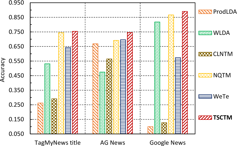
Figure 3: Text classification results with topic distributions learned by topic models.

5.3 Short Text Clustering

Apart from topic quality, we evaluate the quality of inferred topic distributions through short text clustering following Wang et al. (2022). Specifically, we use the most significant topics in the learned topic distributions of short texts as their cluster assignments. Then, we employ the commonly-used clustering metrics, Purity and NMI Manning et al. (2008) to measure the clustering performance as Wang et al. (2022). Note that our goal is not to achieve state-of-the-art clustering performance but to compare the quality of learned topic distributions. Table 4 shows that the clustering performance of our model is generally the best over baseline models concerning both Purity and NMI. This demonstrates that our model can infer more accurate topic distributions of short texts.

5.4 Short Text Classification

In order to compare extrinsic performance, we conduct text classification experiments as a downstream task of topic models Nguyen and Luu (2021). In detail, we use the learned topic distributions by different models as features and train SVM classifiers to predict the class of each short text. We use the labels from the adopted datasets. Figure 3 shows that our TSCTM consistently achieves the best classification performance compared to baseline models. Note that the p-values of significance tests are all less than 0.05. This shows that the learned topic distributions of our model are more discriminative and accordingly can be better employed in the text classification downstream task.

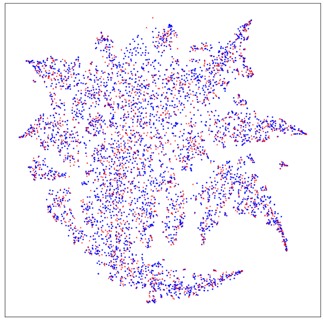
(a) ProdLDA

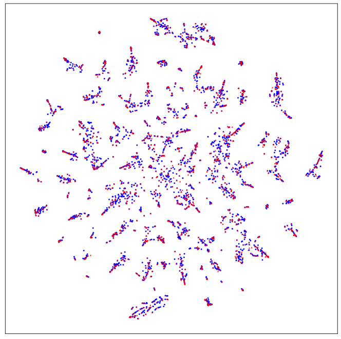
(b) NQTM

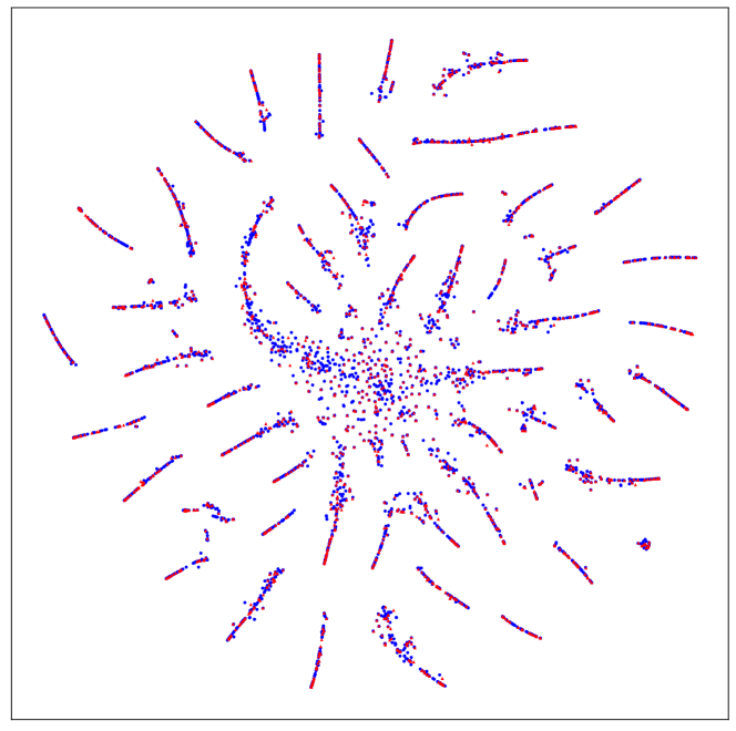
(c) TSCTM

Figure 4: t-SNE visualization of learned topic distributions of original ( $\blacktriangle$) and augmented ( $\bullet$) short texts. Compared to ProdLDA and NQTM, the points of TSCTM are better aggregated and separately scattered in the space.

Model	TagMyNews title			AG News			Google News
	$K$=50	$K$=100		$K$=50	$K$=100		$K$=50	$K$=100
ProdLDA	0.412	0.272		0.612	0.549		0.304	0.433
WLDA	0.640	0.620		0.860	0.866		0.887	0.870
CLNTM	0.541	0.477		0.425	0.405		0.572	0.511
NQTM	0.870	0.858		0.962	0.963		0.947	0.942
WeTe	0.839	0.816		0.938	0.926		0.914	0.907
TSCTM	0.946	0.945		0.986	0.987		0.974	0.974

Table 5: Cosine similarity between topic distributions of original and augmented short texts. The highest are in bold.

5.5 Analysis of Topic Distributions

In this section we analyze the learned topic distributions of short texts to evaluate the modeling of relations among samples. Figure 4 illustrates the t-SNE van der Maaten and Hinton (2008) visualization for the learned topic distributions of original and augmented short texts by ProdLDA, NQTM, and our TSCTM. It shows that the topic distributions learned by our TSCTM are more aggregated together and well separately scattered in the space, in terms of only original short texts or both original and augmented short texts. In addition, we report the cosine similarity between the topic distributions of original and augmented short texts in Table 5. Their similarity should be high since they have similar semantics. We see that TSCTM has the highest similarity among all models. These are because TSCTM can sufficiently model the relations among samples with the novel topic-semantic contrastive learning, which refines the representations and thus topic distributions. These results can further demonstrate the effectiveness of our proposed topic-semantic contrastive learning method.

6 Conclusion

In this paper, we propose TSCTM, a novel and unified method for topic modeling of short texts. Our method with the novel topic-semantic contrastive learning can refine the learning of representations through sufficiently modeling the relations among texts, regardless of the data augmentation availability. Experiments show our model effectively alleviates the data sparsity issue and consistently outperforms state-of-the-art baselines, generating high-quality topics and deriving useful topic distributions of short texts.

Limitations

Our method achieves promising performance to mitigate data sparsity for short text topic modeling, but we believe that there are two limitations to be explored for future works: (i) More data augmentation techniques may be studied to further improve short text topic modeling performance. (ii) The possible metadata of short texts, like authors, hashtags, and sentiments, can be considered to further assist the modeling of relations.

Models	Examples of Topics
ProdLDA	perrish apps chart giraffe cleared lash mary tyrese fill fundamentalist
	blog mistake duel reduce sleet giraffe animation tradition stress freezing
	major giraffe offence moment halo lifetime jim sharing draft congo
NQTM	kanye west confirms yeezus adidas leaf album rant concert kravitz
	kim west kanye invited brody jenner kardashian wedding beautiful invite
	kanye james video west bound recreate kimye franco shot music
TSCTM	giraffe congo poaching forgotten habitat ape okapi bonobo specie endangered
	frozen disney animation idina menzel kristen animated melt fairy bell
	adidas nike partnership summer lenny kravitz confirms cruel kanye album

Table 6: Top 10 related words of discovered topics from Google News. Repetitive words are underlined.

Appendix A Model Implementation

We conduct experiments on NVIDIA GPU, and it takes less than 0.5 GPU hours to train our model on each dataset. For our model, the encoder network $f_{\Theta}$ is a two-layer MLP with softplus as the activation function, same as Wu et al. (2020b), and we use Adam Kingma and Ba (2014) to optimize model parameters. We run our model for 200 epochs with learning rate as 0.002 following Srivastava and Sutton (2017), and $\lambda$ as 0.1 following van den Oord and Vinyals (2017).

Appendix B Examples of Discovered Topics

Following Nan et al. (2019); Wu et al. (2020b), we randomly select some examples of discovered topics by ProdLDA, NQTM, and our TSCTM from Google News for qualitative study since they perform relatively better among baselines. As shown in Table 6, ProdLDA produces several redundant topics including “giraffe”, and these topics are less informative as they are associated with irrelevant words like “fundamentalist” and “animation”. NQTM also has repetitive topics about “kanye”. In contrast, our TSCTM only generates one coherent topic about “animation”, “kanye”, and “giraffe” with relevant words. For example, the topic of TSCTM is more focused on “animation” with “disney”, the movie name “frozen” and its theme song singer “idina menzel”.

References

- Blei et al. (2017) David M Blei, Alp Kucukelbir, and Jon D McAuliffe. 2017. Variational inference: A review for statisticians. Journal of the American statistical Association, 112(518):859–877.
- Blei et al. (2003) David M Blei, Andrew Y Ng, and Michael I Jordan. 2003. Latent dirichlet allocation. Journal of Machine Learning Research, 3(Jan):993–1022.
- Boyd-Graber et al. (2017) Jordan L Boyd-Graber, Yuening Hu, David Mimno, et al. 2017. Applications of topic models, volume 11. now Publishers Incorporated.
- Card et al. (2018) Dallas Card, Chenhao Tan, and Noah A Smith. 2018. Neural Models for Documents with Metadata. In Proceedings of the 56th Annual Meeting of the Association for Computational Linguistics (Volume 1: Long Papers), volume 1, pages 2031–2040.
- Chen and Kao (2015) Guan-Bin Chen and Hung-Yu Kao. 2015. Word co-occurrence augmented topic model in short text. In International Journal of Computational Linguistics & Chinese Language Processing, Volume 20, Number 2, December 2015-Special Issue on Selected Papers from ROCLING XXVII.
- Chen et al. (2020) Ting Chen, Simon Kornblith, Mohammad Norouzi, and Geoffrey Hinton. 2020. A simple framework for contrastive learning of visual representations. In International conference on machine learning, pages 1597–1607. PMLR.
- Devlin et al. (2018) Jacob Devlin, Ming-Wei Chang, Kenton Lee, and Kristina Toutanova. 2018. Bert: Pre-training of deep bidirectional transformers for language understanding. arXiv preprint arXiv:1810.04805.
- Dieng et al. (2020) Adji B Dieng, Francisco JR Ruiz, and David M Blei. 2020. Topic modeling in embedding spaces. Transactions of the Association for Computational Linguistics, 8:439–453.
- Frosst et al. (2019) Nicholas Frosst, Nicolas Papernot, and Geoffrey Hinton. 2019. Analyzing and improving representations with the soft nearest neighbor loss. In International conference on machine learning, pages 2012–2020. PMLR.
- Gao et al. (2021) Tianyu Gao, Xingcheng Yao, and Danqi Chen. 2021. Simcse: Simple contrastive learning of sentence embeddings. arXiv preprint arXiv:2104.08821.
- Griffiths and Steyvers (2004) Thomas L Griffiths and Mark Steyvers. 2004. Finding scientific topics. Proceedings of the National academy of Sciences, 101(suppl 1):5228–5235.
- Hadsell et al. (2006) Raia Hadsell, Sumit Chopra, and Yann LeCun. 2006. Dimensionality reduction by learning an invariant mapping. In 2006 IEEE Computer Society Conference on Computer Vision and Pattern Recognition (CVPR’06), volume 2, pages 1735–1742. IEEE.
- He et al. (2020) Kaiming He, Haoqi Fan, Yuxin Wu, Saining Xie, and Ross Girshick. 2020. Momentum contrast for unsupervised visual representation learning. In Proceedings of the IEEE/CVF conference on computer vision and pattern recognition, pages 9729–9738.
- Hjelm et al. (2018) R Devon Hjelm, Alex Fedorov, Samuel Lavoie-Marchildon, Karan Grewal, Phil Bachman, Adam Trischler, and Yoshua Bengio. 2018. Learning deep representations by mutual information estimation and maximization. arXiv preprint arXiv:1808.06670.
- Hofmann (1999) Thomas Hofmann. 1999. Probabilistic latent semantic analysis. In Proceedings of the Fifteenth conference on Uncertainty in artificial intelligence, pages 289–296. Morgan Kaufmann Publishers Inc.
- Jin et al. (2011) Ou Jin, Nathan N Liu, Kai Zhao, Yong Yu, and Qiang Yang. 2011. Transferring topical knowledge from auxiliary long texts for short text clustering. In Proceedings of the 20th ACM international conference on Information and knowledge management, pages 775–784. ACM.
- Khosla et al. (2020) Prannay Khosla, Piotr Teterwak, Chen Wang, Aaron Sarna, Yonglong Tian, Phillip Isola, Aaron Maschinot, Ce Liu, and Dilip Krishnan. 2020. Supervised contrastive learning. arXiv preprint arXiv:2004.11362.
- Kingma and Ba (2014) Diederik P Kingma and Jimmy Ba. 2014. Adam: A method for stochastic optimization. arXiv preprint arXiv:1412.6980.
- Kingma and Welling (2014) Diederik P Kingma and Max Welling. 2014. Auto-encoding variational bayes. In The International Conference on Learning Representations (ICLR).
- Kobayashi (2018) Sosuke Kobayashi. 2018. Contextual augmentation: Data augmentation by words with paradigmatic relations. In NAACL-HLT (2).
- Lee et al. (2020) Moontae Lee, David Bindel, and David Mimno. 2020. Prior-aware composition inference for spectral topic models. In International Conference on Artificial Intelligence and Statistics, pages 4258–4268. PMLR.
- Li et al. (2016) Chenliang Li, Haoran Wang, Zhiqian Zhang, Aixin Sun, and Zongyang Ma. 2016. Topic modeling for short texts with auxiliary word embeddings. In Proceedings of the 39th International ACM SIGIR conference on Research and Development in Information Retrieval, pages 165–174. ACM.
- Li et al. (2021) Ximing Li, Yang Wang, Jihong Ouyang, and Meng Wang. 2021. Topic extraction from extremely short texts with variational manifold regularization. Machine Learning, 110(5):1029–1066.
- Ma (2019) Edward Ma. 2019. Nlp augmentation. https://github.com/makcedward/nlpaug.
- Ma et al. (2012) Zongyang Ma, Aixin Sun, Quan Yuan, and Gao Cong. 2012. Topic-driven reader comments summarization. In Proceedings of the 21st ACM international conference on Information and knowledge management, pages 265–274. ACM.
- Manning et al. (2008) Christopher D Manning, Prabhakar Raghavan, and Hinrich Schütze. 2008. Introduction to Information Retrieval. Cambridge University Press, New York, NY, USA.
- Mehrotra et al. (2013) Rishabh Mehrotra, Scott Sanner, Wray Buntine, and Lexing Xie. 2013. Improving LDA topic models for microblogs via tweet pooling and automatic labeling. In Proceedings of the 36th international ACM SIGIR conference on Research and development in information retrieval, pages 889–892. ACM.
- Miao et al. (2017) Yishu Miao, Edward Grefenstette, and Phil Blunsom. 2017. Discovering discrete latent topics with neural variational inference. In Proceedings of the 34th International Conference on Machine Learning-Volume 70, pages 2410–2419. JMLR. org.
- Miao et al. (2016) Yishu Miao, Lei Yu, and Phil Blunsom. 2016. Neural variational inference for text processing. In International conference on machine learning, pages 1727–1736.
- Nan et al. (2019) Feng Nan, Ran Ding, Ramesh Nallapati, and Bing Xiang. 2019. Topic modeling with Wasserstein autoencoders. In Proceedings of the 57th Annual Meeting of the Association for Computational Linguistics, pages 6345–6381, Florence, Italy. Association for Computational Linguistics.
- Nguyen and Luu (2021) Thong Nguyen and Anh Tuan Luu. 2021. Contrastive learning for neural topic model. Advances in Neural Information Processing Systems, 34.
- Oh Song et al. (2016) Hyun Oh Song, Yu Xiang, Stefanie Jegelka, and Silvio Savarese. 2016. Deep metric learning via lifted structured feature embedding. In Proceedings of the IEEE conference on computer vision and pattern recognition, pages 4004–4012.
- Phan et al. (2008) Xuan-Hieu Phan, Le-Minh Nguyen, and Susumu Horiguchi. 2008. Learning to classify short and sparse text & web with hidden topics from large-scale data collections. In Proceedings of the 17th international conference on World Wide Web, pages 91–100. ACM.
- Qiang et al. (2020) Jipeng Qiang, Zhenyu Qian, Yun Li, Yunhao Yuan, and Xindong Wu. 2020. Short text topic modeling techniques, applications, and performance: a survey. IEEE Transactions on Knowledge and Data Engineering.
- Rakib et al. (2020) Md Rashadul Hasan Rakib, Norbert Zeh, Magdalena Jankowska, and Evangelos Milios. 2020. Enhancement of short text clustering by iterative classification. In International Conference on Applications of Natural Language to Information Systems, pages 105–117. Springer.
- Rezende et al. (2014) Danilo Jimenez Rezende, Shakir Mohamed, and Daan Wierstra. 2014. Stochastic backpropagation and approximate inference in deep generative models. In Proceedings ofthe 31th International Conference on Machine Learning.
- Röder et al. (2015) Michael Röder, Andreas Both, and Alexander Hinneburg. 2015. Exploring the space of topic coherence measures. In Proceedings of the eighth ACM international conference on Web search and data mining, pages 399–408. ACM.
- Srivastava and Sutton (2017) Akash Srivastava and Charles Sutton. 2017. Autoencoding variational inference for topic models. In ICLR.
- Tolstikhin et al. (2018) Ilya Tolstikhin, Olivier Bousquet, Sylvain Gelly, and Bernhard Schoelkopf. 2018. Wasserstein auto-encoders. In International Conference on Learning Representations.
- Van den Oord et al. (2018) Aaron Van den Oord, Yazhe Li, and Oriol Vinyals. 2018. Representation learning with contrastive predictive coding. arXiv e-prints, pages arXiv–1807.
- van den Oord and Vinyals (2017) Aaron van den Oord and Oriol Vinyals. 2017. Neural discrete representation learning. In Advances in Neural Information Processing Systems, pages 6306–6315.
- van der Maaten and Hinton (2008) Laurens van der Maaten and Geoffrey Hinton. 2008. Visualizing data using t-SNE. Journal of machine learning research, 9(Nov):2579–2605.
- Vitale et al. (2012) Daniele Vitale, Paolo Ferragina, and Ugo Scaiella. 2012. Classification of short texts by deploying topical annotations. In European Conference on Information Retrieval, pages 376–387. Springer.
- Wang et al. (2022) Dongsheng Wang, Dandan Guo, He Zhao, Huangjie Zheng, Korawat Tanwisuth, Bo Chen, and Mingyuan Zhou. 2022. Representing mixtures of word embeddings with mixtures of topic embeddings. In International Conference on Learning Representations.
- Wang and Isola (2020) Tongzhou Wang and Phillip Isola. 2020. Understanding contrastive representation learning through alignment and uniformity on the hypersphere. In International Conference on Machine Learning, pages 9929–9939. PMLR.
- Wang et al. (2019) Xun Wang, Xintong Han, Weilin Huang, Dengke Dong, and Matthew R Scott. 2019. Multi-similarity loss with general pair weighting for deep metric learning. In Proceedings of the IEEE/CVF Conference on Computer Vision and Pattern Recognition, pages 5022–5030.
- Wang et al. (2021) Yiming Wang, Ximing Li, Xiaotang Zhou, and Jihong Ouyang. 2021. Extracting topics with simultaneous word co-occurrence and semantic correlation graphs: Neural topic modeling for short texts. In Findings of the Association for Computational Linguistics: EMNLP 2021, pages 18–27.
- Wu and Li (2019) Xiaobao Wu and Chunping Li. 2019. Short Text Topic Modeling with Flexible Word Patterns. In International Joint Conference on Neural Networks.
- Wu et al. (2021) Xiaobao Wu, Chunping Li, and Yishu Miao. 2021. Discovering topics in long-tailed corpora with causal intervention. In Findings of the Association for Computational Linguistics: ACL-IJCNLP 2021, pages 175–185, Online. Association for Computational Linguistics.
- Wu et al. (2020a) Xiaobao Wu, Chunping Li, Yan Zhu, and Yishu Miao. 2020a. Learning Multilingual Topics with Neural Variational Inference. In International Conference on Natural Language Processing and Chinese Computing.
- Wu et al. (2020b) Xiaobao Wu, Chunping Li, Yan Zhu, and Yishu Miao. 2020b. Short text topic modeling with topic distribution quantization and negative sampling decoder. In Proceedings of the 2020 Conference on Empirical Methods in Natural Language Processing (EMNLP), pages 1772–1782, Online.
- Wu et al. (2018) Zhirong Wu, Yuanjun Xiong, Stella X Yu, and Dahua Lin. 2018. Unsupervised feature learning via non-parametric instance discrimination. In Proceedings of the IEEE conference on computer vision and pattern recognition, pages 3733–3742.
- Xie et al. (2021) Enze Xie, Jian Ding, Wenhai Wang, Xiaohang Zhan, Hang Xu, Peize Sun, Zhenguo Li, and Ping Luo. 2021. Detco: Unsupervised contrastive learning for object detection. In Proceedings of the IEEE/CVF International Conference on Computer Vision, pages 8392–8401.
- Yan et al. (2013) Xiaohui Yan, Jiafeng Guo, Yanyan Lan, and Xueqi Cheng. 2013. A biterm topic model for short texts. In Proceedings of the 22nd international conference on World Wide Web, pages 1445–1456. ACM.
- Yin and Wang (2014) Jianhua Yin and Jianyong Wang. 2014. A dirichlet multinomial mixture model-based approach for short text clustering. In Proceedings of the 20th ACM SIGKDD international conference on Knowledge discovery and data mining, pages 233–242. ACM.
- Zhang et al. (2021) Dejiao Zhang, Feng Nan, Xiaokai Wei, Shang-Wen Li, Henghui Zhu, Kathleen McKeown, Ramesh Nallapati, Andrew O Arnold, and Bing Xiang. 2021. Supporting clustering with contrastive learning. In Proceedings of the 2021 Conference of the North American Chapter of the Association for Computational Linguistics: Human Language Technologies, pages 5419–5430.
- Zhang et al. (2015) Xiang Zhang, Junbo Zhao, and Yann LeCun. 2015. Character-level convolutional networks for text classification. In Advances in neural information processing systems, pages 649–657.
- Zhao et al. (2021) Xiangyun Zhao, Raviteja Vemulapalli, Philip Andrew Mansfield, Boqing Gong, Bradley Green, Lior Shapira, and Ying Wu. 2021. Contrastive learning for label efficient semantic segmentation. In Proceedings of the IEEE/CVF International Conference on Computer Vision, pages 10623–10633.