DETRs with Collaborative Hybrid Assignments Training

Abstract

In this paper, we provide the observation that too few queries assigned as positive samples in DETR with one-to-one set matching leads to sparse supervision on the encoder’s output which considerably hurt the discriminative feature learning of the encoder and vice visa for attention learning in the decoder. To alleviate this, we present a novel collaborative hybrid assignments training scheme, namely $\mathcal{C}$o-DETR, to learn more efficient and effective DETR-based detectors from versatile label assignment manners. This new training scheme can easily enhance the encoder’s learning ability in end-to-end detectors by training the multiple parallel auxiliary heads supervised by one-to-many label assignments such as ATSS and Faster RCNN. In addition, we conduct extra customized positive queries by extracting the positive coordinates from these auxiliary heads to improve the training efficiency of positive samples in the decoder. In inference, these auxiliary heads are discarded and thus our method introduces no additional parameters and computational cost to the original detector while requiring no hand-crafted non-maximum suppression (NMS). We conduct extensive experiments to evaluate the effectiveness of the proposed approach on DETR variants, including DAB-DETR, Deformable-DETR, and DINO-Deformable-DETR. The state-of-the-art DINO-Deformable-DETR with Swin-L can be improved from 58.5% to 59.5% AP on COCO val. Surprisingly, incorporated with ViT-L backbone, we achieve 66.0% AP on COCO test-dev and 67.9% AP on LVIS val, outperforming previous methods by clear margins with much fewer model sizes. Codes are available at https://github.com/Sense-X/Co-DETR.

1 Introduction

Figure 1: Performance of models with ResNet-50 on COCO val. $\mathcal{C}$o-DETR outperforms other counterparts by a large margin.

Object detection is a fundamental task in computer vision, which requires us to localize the object and classify its category. The seminal R-CNN families [11, 27, 14] and a series of variants [31, 44, 37] such as ATSS [41], RetinaNet [21], FCOS [32], and PAA [17] lead to the significant breakthrough of object detection task. One-to-many label assignment is the core scheme of them, where each ground-truth box is assigned to multiple coordinates in the detector’s output as the supervised target cooperated with proposals [11, 27], anchors [21] or window centers [32]. Despite their promising performance, these detectors heavily rely on many hand-designed components like a non-maximum suppression procedure or anchor generation [1]. To conduct a more flexible end-to-end detector, DEtection TRansformer (DETR) [1] is proposed to view the object detection as a set prediction problem and introduce the one-to-one set matching scheme based on a transformer encoder-decoder architecture. In this manner, each ground-truth box will only be assigned to one specific query, and multiple hand-designed components that encode prior knowledge are no longer needed. This approach introduces a flexible detection pipeline and encourages many DETR variants to further improve it. However, the performance of the vanilla end-to-end object detector is still inferior to the traditional detectors with one-to-many label assignments.

Figure 2: IoF-IoB curves for the feature discriminability score in the encoder and attention discriminability score in the decoder.

In this paper, we try to make DETR-based detectors superior to conventional detectors while maintaining their end-to-end merit. To address this challenge, we focus on the intuitive drawback of one-to-one set matching that it explores less positive queries. This will lead to severe inefficient training issues. We detailedly analyze this from two aspects, the latent representation generated by the encoder and the attention learning in the decoder. We first compare the discriminability score of the latent features between the Deformable-DETR [43] and the one-to-many label assignment method where we simply replace the decoder with the ATSS head. The feature $l^{2}$-norm in each spatial coordinate is utilized to represent the discriminability score. Given the encoder’s output $\mathcal{F}\in\mathbb{R}^{C\times H\times W}$, we can obtain the discriminability score map $\mathcal{S}\in\mathbb{R}^{1\times H\times W}$. The object can be better detected when the scores in the corresponding area are higher. As shown in Figure 2, we demonstrate the IoF-IoB curve (IoF: intersection over foreground, IoB: intersection over background) by applying different thresholds on the discriminability scores (details in Section 3.4). The higher IoF-IoB curve in ATSS indicates that it’s easier to distinguish the foreground and background. We further visualize the discriminability score map $\mathcal{S}$ in Figure 3. It’s obvious that the features in some salient areas are fully activated in the one-to-many label assignment method but less explored in one-to-one set matching. For the exploration of decoder training, we also demonstrate the IoF-IoB curve of the cross-attention score in the decoder based on the Deformable-DETR and the Group-DETR [5] which introduces more positive queries into the decoder. The illustration in Figure 2 shows that too few positive queries also influence attention learning and increasing more positive queries in the decoder can slightly alleviate this.

This significant observation motivates us to present a simple but effective method, a collaborative hybrid assignment training scheme ($\mathcal{C}$o-DETR). The key insight of $\mathcal{C}$o-DETR is to use versatile one-to-many label assignments to improve the training efficiency and effectiveness of both the encoder and decoder. More specifically, we integrate the auxiliary heads with the output of the transformer encoder. These heads can be supervised by versatile one-to-many label assignments such as ATSS [41], FCOS [32], and Faster RCNN  [27]. Different label assignments enrich the supervisions on the encoder’s output which forces it to be discriminative enough to support the training convergence of these heads. To further improve the training efficiency of the decoder, we elaborately encode the coordinates of positive samples in these auxiliary heads, including the positive anchors and positive proposals. They are sent to the original decoder as multiple groups of positive queries to predict the pre-assigned categories and bounding boxes. Positive coordinates in each auxiliary head serve as an independent group that is isolated from the other groups. Versatile one-to-many label assignments can introduce lavish (positive query, ground-truth) pairs to improve the decoder’s training efficiency. Note that, only the original decoder is used during inference, thus the proposed training scheme only introduces extra overheads during training.

Figure 3: Visualizations of discriminability scores in the encoder.

We conduct extensive experiments to evaluate the efficiency and effectiveness of the proposed method. Illustrated in Figure 3, $\mathcal{C}$o-DETR greatly alleviates the poorly encoder’s feature learning in one-to-one set matching. As a plug-and-play approach, we easily combine it with different DETR variants, including DAB-DETR [23], Deformable-DETR [43], and DINO-Deformable-DETR [39]. As shown in Figure 1, $\mathcal{C}$o-DETR achieves faster training convergence and even higher performance. Specifically, we improve the basic Deformable-DETR by 5.8% AP in 12-epoch training and 3.2% AP in 36-epoch training. The state-of-the-art DINO-Deformable-DETR with Swin-L [25] can still be improved from 58.5% to 59.5% AP on COCO val. Surprisingly, incorporated with ViT-L [8] backbone, we achieve 66.0% AP on COCO test-dev and 67.9% AP on LVIS val, establishing the new state-of-the-art detector with much fewer model sizes.

2 Related Works

Figure 4: Framework of our Collaborative Hybrid Assignment Training. The auxiliary branches are discarded during evaluation.

One-to-many label assignment. For one-to-many label assignment in object detection, multiple box candidates can be assigned to the same ground-truth box as positive samples in the training phase. In classic anchor-based detectors, such as Faster-RCNN [27] and RetinaNet [21], the sample selection is guided by the predefined IoU threshold and matching IoU between anchors and annotated boxes. The anchor-free FCOS [32] leverages the center priors and assigns spatial locations near the center of each bounding box as positives. Moreover, the adaptive mechanism is incorporated into one-to-many label assignments to overcome the limitation of fixed label assignments. ATSS [41] performs adaptive anchor selection by the statistical dynamic IoU values of top-$k$ closest anchors. PAA [17] adaptively separates anchors into positive and negative samples in a probabilistic manner. In this paper, we propose a collaborative hybrid assignment scheme to improve encoder representations via auxiliary heads with one-to-many label assignments.

One-to-one set matching. The pioneering transformer-based detector, DETR [1], incorporates the one-to-one set matching scheme into object detection and performs fully end-to-end object detection. The one-to-one set matching strategy first calculates the global matching cost via Hungarian matching and assigns only one positive sample with the minimum matching cost for each ground-truth box. DN-DETR [18] demonstrates the slow convergence results from the instability of one-to-one set matching, thus introducing denoising training to eliminate this issue. DINO [39] inherits the advanced query formulation of DAB-DETR [23] and incorporates an improved contrastive denoising technique to achieve state-of-the-art performance. Group-DETR [5] constructs group-wise one-to-many label assignment to exploit multiple positive object queries, which is similar to the hybrid matching scheme in $\mathcal{H}$-DETR [16]. In contrast with the above follow-up works, we present a new perspective of collaborative optimization for one-to-one set matching.

3 Method

3.1 Overview

Following the standard DETR protocol, the input image is fed into the backbone and encoder to generate latent features. Multiple predefined object queries interact with them in the decoder via cross-attention afterwards. We introduce $\mathcal{C}$o-DETR to improve the feature learning in the encoder and the attention learning in the decoder via the collaborative hybrid assignments training scheme and the customized positive queries generation. We will detailedly describe these modules and give insights why they can work well.

Head $i$	Loss $\mathcal{L}_{i}$	Assignment $\mathcal{A}_{i}$
		${\{pos\}}$, ${\{neg\}}$ Generation	$\mathbf{P}_{i}$ Generation	$\mathbf{B}_{i}^{\{pos\}}$ Generation
Faster-RCNN [27]	cls: CE loss,	$\{pos\}$: IoU(proposal, gt)>$0.5$	$\{pos\}$: gt labels, offset(proposal, gt)	positive proposals
	reg: GIoU loss	$\{neg\}$: IoU(proposal, gt)<$0.5$	$\{neg\}$: gt labels	$(x_{1},y_{1},x_{2},y_{2})$
ATSS [41]	cls: Focal loss	$\{pos\}$:IoU(anchor, gt)>(mean+std)	$\{pos\}$: gt labels, offset(anchor, gt), centerness	positive anchors
	reg: GIoU, BCE loss	$\{neg\}$: IoU(anchor, gt)<(mean+std)	$\{neg\}$: gt labels	$(x_{1},y_{1},x_{2},y_{2})$
RetinaNet [21]	cls: Focal loss	$\{pos\}$: IoU(anchor, gt)>$0.5$	$\{pos\}$: gt labels, offset(anchor, gt)	positive anchors
	reg: GIoU Loss	$\{neg\}$: IoU(anchor, gt)<$0.4$	$\{neg\}$: gt labels	$(x_{1},y_{1},x_{2},y_{2})$
FCOS [32]	cls: Focal Loss	$\{pos\}$: points inside gt center area	$\{pos\}$: gt labels, ltrb distance, centerness	FCOS point $(cx,cy)$
	reg: GIoU, BCE loss	$\{neg\}$: points outside gt center area	$\{neg\}$: gt labels	$w=h=8\times 2^{2+j}$

Table 1: Detailed information of auxiliary heads. The auxiliary heads include Faster-RCNN [27], ATSS [41], RetinaNet [21], and FCOS [32]. If not otherwise specified, we follow the original implementations, e.g., anchor generation.

3.2 Collaborative Hybrid Assignments Training

To alleviate the sparse supervision on the encoder’s output caused by the fewer positive queries in the decoder, we incorporate versatile auxiliary heads with different one-to-many label assignment paradigms, e.g., ATSS, and Faster R-CNN. Different label assignments enrich the supervisions on the encoder’s output which forces it to be discriminative enough to support the training convergence of these heads. Specifically, given the encoder’s latent feature $\mathcal{F}$, we firstly transform it to the feature pyramid $\{\mathcal{F}_{1},\cdots,\mathcal{F}_{J}\}$ via the multi-scale adapter where $J$ indicates feature map with $2^{2+J}$ downsampling stride. Similar to ViTDet [20], the feature pyramid is constructed by a single feature map in the single-scale encoder, while we use bilinear interpolation and $3\times 3$ convolution for upsampling. For instance, with the single-scale feature from the encoder, we successively apply downsampling ($3\times 3$ convolution with stride $2$) or upsampling operations to produce a feature pyramid. As for the multi-scale encoder, we only downsample the coarsest feature in the multi-scale encoder features $\mathcal{F}$ to build the feature pyramid. Defined $K$ collaborative heads with corresponding label assignment manners $\mathcal{A}_{k}$, for the $i$-th collaborative head, $\{\mathcal{F}_{1},\cdots,\mathcal{F}_{J}\}$ is sent to it to obtain the predictions $\mathbf{\hat{P}}_{i}$. At the $i$-th head, $\mathcal{A}_{i}$ is used to compute the supervised targets for the positive and negative samples in $\mathbf{P}_{i}$. Denoted $\mathbf{G}$ as the ground-truth set, this procedure can be formulated as:

$$\mathbf{P}_{i}^{\{pos\}},\mathbf{B}_{i}^{\{pos\}},\mathbf{P}_{i}^{\{neg\}}=\mathcal{A}_{i}(\mathbf{\hat{P}}_{i},\mathbf{G}),$$ (1)

where ${\{pos\}}$ and ${\{neg\}}$ indicate the pair set of ($j$, positive coordinates or negative coordinates in $\mathcal{F}_{j}$) determined by $\mathcal{A}_{i}$. $j$ means the feature index in $\{\mathcal{F}_{1},\cdots,\mathcal{F}_{J}\}$. $\mathbf{B}_{i}^{\{pos\}}$ is the set of spatial positive coordinates. $\mathbf{P}_{i}^{\{pos\}}$ and $\mathbf{P}_{i}^{\{neg\}}$ are the supervised targets in the corresponding coordinates, including the categories and regressed offsets. To be specific, we describe the detailed information about each variable in Table 1. The loss functions can be defined as:

$$\mathcal{L}^{enc}_{i}=\mathcal{L}_{i}(\mathbf{\hat{P}}_{i}^{\{pos\}},\mathbf{{P}}_{i}^{\{pos\}})+\mathcal{L}_{i}(\mathbf{\hat{P}}_{i}^{\{neg\}},\mathbf{{P}}_{i}^{\{neg\}}),$$ (2)

Note that the regression loss is discarded for negative samples. The training objective of the optimization for $K$ auxiliary heads is formulated as follows:

$$\mathcal{L}^{enc}=\sum_{i=1}^{K}\mathcal{L}_{i}^{enc}$$ (3)

3.3 Customized Positive Queries Generation

In the one-to-one set matching paradigm, each ground-truth box will only be assigned to one specific query as the supervised target. Too few positive queries lead to inefficient cross-attention learning in the transformer decoder as shown in Figure 2. To alleviate this, we elaborately generate sufficient customized positive queries according to the label assignment $\mathcal{A}_{i}$ in each auxiliary head. Specifically, given the positive coordinates set $\mathbf{B}_{i}^{\{pos\}}\in\mathbb{R}^{M_{i}\times 4}$ in the $i$-th auxiliary head, where $M_{i}$ is the number of positive samples, the extra customized positive queries $\mathbf{Q}_{i}\in\mathbb{R}^{M_{i}\times C}$ can be generated by:

$$\mathbf{Q}_{i}=\mathrm{Linear}(\mathrm{PE}(\mathbf{B}_{i}^{\{pos\}}))+\mathrm{Linear}(\mathrm{E}(\mathbf{\{\mathcal{F}_{*}\}},{\{pos\}})).$$ (4)

where $\mathrm{PE}(\cdot)$ stands for positional encodings and we select the corresponding features from $\mathrm{E}(\cdot)$ according to the index pair ($j$, positive coordinates or negative coordinates in $\mathcal{F}_{j}$).

As a result, there are $K+1$ groups of queries that contribute to a single one-to-one set matching branch and $K$ branches with one-to-many label assignments during training. The auxiliary one-to-many label assignment branches share the same parameters with $L$ decoders layers in the original main branch. All the queries in the auxiliary branch are regarded as positive queries, thus the matching process is discarded. To be specific, the loss of the $l$-th decoder layer in the $i$-th auxiliary branch can be formulated as:

$$\mathcal{L}^{dec}_{i,l}=\widetilde{\mathcal{L}}(\widetilde{\mathbf{P}}_{i,l},\mathbf{{P}}_{i}^{\{pos\}}).$$ (5)

$\widetilde{\mathbf{P}}_{i,l}$ refers to the output predictions of the $l$-th decoder layer in the $i$-th auxiliary branch. Finally, the training objective for $\mathcal{C}$o-DETR is:

$$\mathcal{L}^{global}=\sum_{l=1}^{L}(\widetilde{\mathcal{L}}^{dec}_{l}+\lambda_{1}\sum_{i=1}^{K}\mathcal{L}^{dec}_{i,l}+\lambda_{2}\mathcal{L}^{enc}),$$ (6)

where $\widetilde{\mathcal{L}}^{dec}_{l}$ stands for the loss in the original one-to-one set matching branch [1], $\lambda_{1}$ and $\lambda_{2}$ are the coefficient balancing the losses.

3.4 Why Co-DETR works

$\mathcal{C}$o-DETR leads to evident improvement to the DETR-based detectors. In the following, we try to investigate its effectiveness qualitatively and quantitatively. We conduct detailed analysis based on Deformable-DETR with ResNet-50 [15] backbone using the 36-epoch setting.

Enrich the encoder’s supervisions. Intuitively, too few positive queries lead to sparse supervisions as only one query is supervised by regression loss for each ground-truth. The positive samples in one-to-many label assignment manners receive more localization supervisions to help enhance the latent feature learning. To further explore how the sparse supervisions impede the model training, we detailedly investigate the latent features produced by the encoder. We introduce the IoF-IoB curve to quantize the discriminability score of the encoder’s output. Specifically, given the latent feature $\mathcal{F}$ of the encoder, inspired by the feature visualization in Figure 3, we compute the IoF (intersection over foreground) and IoB (intersection over background). Given the encoder’s feature $\mathcal{F}_{j}\in\mathbb{R}^{C\times H_{j}\times W_{j}}$ at level $j$, we first calculate the $l^{2}$-norm $\widehat{\mathcal{F}}_{j}\in\mathbb{R}^{1\times H_{j}\times W_{j}}$ and resize it to the image size $H\times W$. The discriminability score $\mathcal{D}(\mathcal{F})$ is computed by averaging the scores from all levels:

$$\mathcal{D}(\mathcal{F})=\frac{1}{J}\sum_{j=1}^{J}\frac{\widehat{\mathcal{F}}_{j}}{max(\widehat{\mathcal{F}}_{j})},$$ (7)

where the resize operation is omitted. We visualize the discriminability scores of ATSS, Deformable-DETR, and our $\mathcal{C}$o-Deformable-DETR in Figure 3. Compared with Deformable-DETR, both ATSS and $\mathcal{C}$o-Deformable-DETR own stronger ability to distinguish the areas of key objects, while Deformable-DETR is almost disturbed by the background. Consequently, we define the indicators for foreground and background as $\mathbbm{1}(\mathcal{D}(\mathcal{F})>S)\in\mathbb{R}^{H\times W}$ and $\mathbbm{1}(\mathcal{D}(\mathcal{F})<S)\in\mathbb{R}^{H\times W}$, respectively. $S$ is a predefined score thresh, $\mathbbm{1}(x)$ is 1 if $x$ is true and 0 otherwise. As for the mask of foreground $\mathcal{M}^{fg}\in\mathbb{R}^{H\times W}$, the element $\mathcal{M}^{fg}_{h,w}$ is 1 if the point $(h,w)$ is inside the foreground and 0 otherwise. The area of intersection over foreground (IoF) $\mathcal{I}^{fg}$ can be computed as:

$$\mathcal{I}^{fg}=\frac{\sum_{h=1}^{H}\sum_{w=1}^{W}(\mathbbm{1}(\mathcal{D}(\mathcal{F}_{h,w})>S)\cdot\mathcal{M}^{fg}_{h,w})}{\sum_{h=1}^{H}\sum_{w=1}^{W}\mathcal{M}^{fg}_{h,w}}.$$ (8)

Concretely, we compute the area of intersection over background areas (IoB) in a similar way and plot the curve IoF and IoB by varying $S$ in Figure 2. Obviously, ATSS and $C$o-Deformable-DETR obtain higher IoF values than both Deformable-DETR and Group-DETR under the same IoB values, which demonstrates the encoder representations benefit from the one-to-many label assignment.

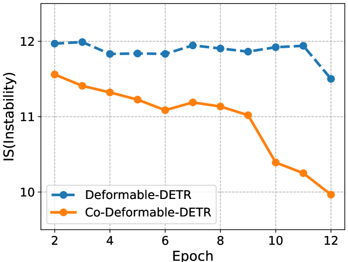
Figure 5: The instability (IS) [18] of Deformable-DETR and $\mathcal{C}$o-Deformable-DETR on COCO dataset. These detectors are trained for 12 epochs with ResNet-50 backbones.

Improve the cross-attention learning by reducing the instability of Hungarian matching. Hungarian matching is the core scheme in one-to-one set matching. Cross-attention is an important operation to help the positive queries encode abundant object information. It requires sufficient training to achieve this. We observe that the Hungarian matching introduces uncontrollable instability since the ground-truth assigned to a specific positive query in the same image is changing during the training process. Following [18], we present the comparison of instability in Figure 5, where we find our approach contributes to a more stable matching process. Furthermore, in order to quantify how well cross-attention is being optimized, we also calculate the IoF-IoB curve for attention score. Similar to the feature discriminability score computation, we set different thresholds for attention score to get multiple IoF-IoB pairs. The comparisons between Deformable-DETR, Group-DETR, and $\mathcal{C}$o-Deformable-DETR can be viewed in Figure 2. We find that the IoF-IoB curves of DETRs with more positive queries are generally above Deformable-DETR, which is consistent with our motivation.

3.5 Comparison with other methods

Differences between our method and other counterparts. Group-DETR, $\mathcal{H}$-DETR, and SQR [2] perform one-to-many assignments by one-to-one matching with duplicate groups and repeated ground-truth boxes. $\mathcal{C}$o-DETR explicitly assigns multiple spatial coordinates as positives for each ground truth. Accordingly, these dense supervision signals are directly applied to the latent feature map to enable it more discriminative. By contrast, Group-DETR, $\mathcal{H}$-DETR, and SQR lack this mechanism. Although more positive queries are introduced in these counterparts, the one-to-many assignments implemented by Hungarian Matching still suffer from the instability issues of one-to-one matching. Our method benefits from the stability of off-the-shelf one-to-many assignments and inherits their specific matching manner between positive queries and ground-truth boxes. Group-DETR and $\mathcal{H}$-DETR fail to reveal the complementarities between one-to-one matching and traditional one-to-many assignment. To our best knowledge, we are the first to give the quantitative and qualitative analysis on the detectors with the traditional one-to-many assignment and one-to-one matching. This helps us better understand their differences and complementarities so that we can naturally improve the DETR’s learning ability by leveraging off-the-shelf one-to-many assignment designs without requiring additional specialized one-to-many design experience.

No negative queries are introduced in the decoder. Duplicate object queries inevitably bring large amounts of negative queries for the decoder and a significant increase in GPU memory. However, our method only processes the positive coordinates in the decoder, thus consuming less memory as shown in Table 7.

4 Experiments

Method	$K$	#epochs	AP
Conditional DETR-C5 [26]	0	36	39.4
Conditional DETR-C5 [26]	1	36	41.5(+2.1)
Conditional DETR-C5 [26]	2	36	41.8(+2.4)
DAB-DETR-C5 [23]	0	36	41.2
DAB-DETR-C5 [23]	1	36	43.1(+1.9)
DAB-DETR-C5 [23]	2	36	43.5(+2.3)
Deformable-DETR [43]	0	12	37.1
Deformable-DETR [43]	1	12	42.3(+5.2)
Deformable-DETR [43]	2	12	42.9(+5.8)
Deformable-DETR [43]	0	36	43.3
Deformable-DETR [43]	1	36	46.8(+3.5)
Deformable-DETR [43]	2	36	46.5(+3.2)

Table 2: Results of plain baselines on COCO val.

4.1 Setup

Datasets and Evaluation Metrics. Our experiments are conducted on the MS COCO 2017 dataset [22] and LVIS v1.0 dataset [12]. The COCO dataset consists of 115K labeled images for training and 5K images for validation. We report the detection results by default on the val subset. The results of our largest model evaluated on the test-dev (20K images) are also reported. LVIS v1.0 is a large-scale and long-tail dataset with 1203 categories for large vocabulary instance segmentation. To verify the scalability of $\mathcal{C}$o-DETR, we further apply it to a large-scale object detection benchmark, namely Objects365 [30]. There are 1.7M labeled images used for training and 80K images for validation in the Objects365 dataset. All results follow the standard mean Average Precision(AP) under IoU thresholds ranging from 0.5 to 0.95 at different object scales.

Implementation Details. We incorporate our $\mathcal{C}$o-DETR into the current DETR-like pipelines and keep the training setting consistent with the baselines. We adopt ATSS and Faster-RCNN as the auxiliary heads for $K=2$ and only keep ATSS for $K=1$. More details about our auxiliary heads can be found in the supplementary materials. We choose the number of learnable object queries to 300 and set $\{\lambda_{1},\lambda_{2}\}$ to $\{1.0,2.0\}$ by default. For $\mathcal{C}$o-DINO-Deformable-DETR++, we use large-scale jitter with copy-paste [10].

4.2 Main Results

In this section, we empirically analyze the effectiveness and generalization ability of $\mathcal{C}$o-DETR on different DETR variants in Table 2 and Table 3. All results are reproduced using mmdetection [4]. We first apply the collaborative hybrid assignments training to single-scale DETRs with C5 features. Surprisingly, both Conditional-DETR and DAB-DETR obtain 2.4% and 2.3% AP gains over the baselines with a long training schedule. For Deformable-DETR with multi-scale features, the detection performance is significantly boosted from 37.1% to 42.9% AP. The overall improvements (+3.2% AP) still hold when the training time is increased to 36 epochs. Moreover, we conduct experiments on the improved Deformable-DETR (denoted as Deformable-DETR++) following [16], where a +2.4% AP gain is observed. The state-of-the-art DINO-Deformable-DETR equipped with our method can achieve 51.2% AP, which is +1.8% AP higher than the competitive baseline.

We further scale up the backbone capacity from ResNet-50 to Swin-L [25] based on two state-of-the-art baselines. As presented in Table 3, $\mathcal{C}$o-DETR achieves 56.9% AP and surpasses the Deformable-DETR++ baseline by a large margin (+1.7% AP). The performance of DINO-Deformable-DETR with Swin-L can still be boosted from 58.5% to 59.5% AP.

Method	$K$	#epochs	AP
Deformable-DETR++ [43]	0	12	47.1
Deformable-DETR++ [43]	1	12	48.7(+1.6)
Deformable-DETR++ [43]	2	12	49.5(+2.4)
DINO-Deformable-DETR† [39]	0	12	49.4
DINO-Deformable-DETR† [39]	1	12	51.0(+1.6)
DINO-Deformable-DETR† [39]	2	12	51.2(+1.8)
Deformable-DETR++‡ [43]	0	12	55.2
Deformable-DETR++‡ [43]	1	12	56.4(+1.2)
Deformable-DETR++‡ [43]	2	12	56.9(+1.7)
DINO-Deformable-DETR†‡ [39]	0	36	58.5
DINO-Deformable-DETR†‡ [39]	1	36	59.3(+0.8)
DINO-Deformable-DETR†‡ [39]	2	36	59.5(+1.0)

Table 3: Results of strong baselines on COCO val. Methods with ${\dagger}$ use 5 feature levels. ${\ddagger}$ refers to Swin-L backbone.

Method	Backbone	Multi-scale	#query	#epochs	AP	AP50	AP75	APS	APM	APL
Conditional-DETR [26]	R50	✗	300	108	43.0	64.0	45.7	22.7	46.7	61.5
Anchor-DETR [35]	R50	✗	300	50	42.1	63.1	44.9	22.3	46.2	60.0
DAB-DETR [23]	R50	✗	900	50	45.7	66.2	49.0	26.1	49.4	63.1
AdaMixer [9]	R50	✓	300	36	47.0	66.0	51.1	30.1	50.2	61.8
Deformable-DETR [43]	R50	✓	300	50	46.9	65.6	51.0	29.6	50.1	61.6
DN-Deformable-DETR [18]	R50	✓	300	50	48.6	67.4	52.7	31.0	52.0	63.7
DINO-Deformable-DETR† [39]	R50	✓	900	12	49.4	66.9	53.8	32.3	52.5	63.9
DINO-Deformable-DETR† [39]	R50	✓	900	36	51.2	69.0	55.8	35.0	54.3	65.3
DINO-Deformable-DETR† [39]	Swin-L (IN-22K)	✓	900	36	58.5	77.0	64.1	41.5	62.3	74.0
Group-DINO-Deformable-DETR [5]	Swin-L (IN-22K)	✓	900	36	58.4	-	-	41.0	62.5	73.9
$\mathcal{H}$-Deformable-DETR [16]	R50	✓	300	12	48.7	66.4	52.9	31.2	51.5	63.5
$\mathcal{H}$-Deformable-DETR [16]	Swin-L (IN-22K)	✓	900	36	57.9	76.8	63.6	42.4	61.9	73.4
$\mathcal{C}$o-Deformable-DETR	R50	✓	300	12	49.5	67.6	54.3	32.4	52.7	63.7
$\mathcal{C}$o-Deformable-DETR	Swin-L (IN-22K)	✓	900	36	58.5	77.1	64.5	42.4	62.4	74.0
$\mathcal{C}$o-DINO-Deformable-DETR†	R50	✓	900	12	52.1	69.4	57.1	35.4	55.4	65.9
$\mathcal{C}$o-DINO-Deformable-DETR†	Swin-L (IN-22K)	✓	900	12	58.9	76.9	64.8	42.6	62.7	75.1
$\mathcal{C}$o-DINO-Deformable-DETR†	Swin-L (IN-22K)	✓	900	24	59.8	77.7	65.5	43.6	63.5	75.5
$\mathcal{C}$o-DINO-Deformable-DETR†	Swin-L (IN-22K)	✓	900	36	60.0	77.7	66.1	44.6	63.9	75.7
$\mathcal{C}$o-DINO-Deformable-DETR++†	R50	✓	900	12	52.1	69.3	57.3	35.4	55.5	67.2
$\mathcal{C}$o-DINO-Deformable-DETR++†	R50	✓	900	36	54.8	72.5	60.1	38.3	58.4	69.6
$\mathcal{C}$o-DINO-Deformable-DETR++†	Swin-L (IN-22K)	✓	900	12	59.3	77.3	64.9	43.3	63.3	75.5
$\mathcal{C}$o-DINO-Deformable-DETR++†	Swin-L (IN-22K)	✓	900	24	60.4	78.3	66.4	44.6	64.2	76.5
$\mathcal{C}$o-DINO-Deformable-DETR++†	Swin-L (IN-22K)	✓	900	36	60.7	78.5	66.7	45.1	64.7	76.4
${\dagger}$: 5 feature levels.

Table 4: Comparison to the state-of-the-art DETR variants on COCO val.

Method	Backbone	enc.	val	test-dev
		#params	$\text{AP}^{box}$	$\text{AP}^{box}$
HTC++ [3]	SwinV2-G [24]	3.0B	62.5	63.1
DINO [39]	Swin-L [25]	218M	63.2	63.3
BEIT3 [33]	ViT-g [7]	1.9B	-	63.7
FD [36]	SwinV2-G [24]	3.0B	-	64.2
DINO [39]	FocalNet-H [38]	746M	64.2	64.3
Group DETRv2 [6]	ViT-H [7]	629M	-	64.5
EVA-02 [8]	ViT-L [7]	304M	64.1	64.5
DINO [39]	InternImage-G [34]	3.0B	65.3	65.5
$\mathcal{C}$o-DETR	ViT-L [7]	304M	65.9	66.0

Table 5: Comparison to the state-of-the-art frameworks on COCO.

4.3 Comparisons with the state-of-the-art

We apply our method with $K=2$ to Deformable-DETR++ and DINO. Besides, the quality focal loss [19] and NMS are adopted for our $\mathcal{C}$o-DINO-Deformable-DETR. We report the comparisons on COCO val in Table 4. Compared with other competitive counterparts, our method converges much faster. For example, $\mathcal{C}$o-DINO-Deformable-DETR readily achieves 52.1% AP when using only 12 epochs with ResNet-50 backbone. Our method with Swin-L can obtain 58.9% AP for 1$\times$ scheduler, even surpassing other state-of-the-art frameworks on 3$\times$ scheduler. More importantly, our best model $\mathcal{C}$o-DINO-Deformable-DETR++ achieves 54.8% AP with ResNet-50 and 60.7% AP with Swin-L under 36-epoch training, outperforming all existing detectors with the same backbone by clear margins.

To further explore the scalability of our method, we extend the backbone capacity to 304 million parameters. This large-scale backbone ViT-L [7] is pre-trained using a self-supervised learning method (EVA-02 [8]). We first pre-train $\mathcal{C}$o-DINO-Deformable-DETR with ViT-L on Objects365 for 26 epochs, then fine-tune it on the COCO dataset for 12 epochs. In the fine-tuning stage, the input resolution is randomly selected between 480$\times$2400 and 1536$\times$2400. The detailed settings are available in supplementary materials. Our results are evaluated with test-time augmentation. Table 5 presents the state-of-the-art comparisons on the COCO test-dev benchmark. With much fewer model sizes (304M parameters), $\mathcal{C}$o-DETR sets a new record of 66.0% AP on COCO test-dev, outperforming the previous best model InternImage-G [34] by +0.5% AP.

We also demonstrate the best results of $\mathcal{C}$o-DETR on the long-tailed LVIS detection dataset. In particular, we use the same $\mathcal{C}$o-DINO-Deformable-DETR++ as the model on COCO but choose FedLoss [42] as the classification loss to remedy the impact of unbalanced data distribution. Here, we only apply bounding boxes supervision and report the object detection results. The comparisons are available in Table 6. $\mathcal{C}$o-DETR with Swin-L yields 56.9% and 62.3% AP on LVIS val and minival, surpassing ViTDet with MAE-pretrained [13] ViT-H and GLIPv2 [40] by +3.5% and +2.5% AP, respectively. We further finetune the Objects365 pretrained $\mathcal{C}$o-DETR on this dataset. Without elaborate test-time augmentation, our approach achieves the best detection performance of 67.9% and 71.9% AP on LVIS val and minival. Compared to the 3-billion parameter InternImage-G with test-time augmentation, we obtain +4.7% and +6.1% AP gains on LVIS val and minival while reducing the model size to 1/10.

Method	Backbone	enc.	val	minival
		#params	$\text{AP}^{box}$	$\text{AP}^{box}$
$\mathcal{H}$-DETR [16]	Swin-L [25]	218M	47.9	-
ViTDet [20]	ViT-L [7]	307M	51.2	-
ViTDet [20]	ViT-H [7]	632M	53.4	-
GLIPv2 [40]	Swin-H [25]	637M	-	59.8
DINO [39]	InternImage-G [34]	3.0B	63.2	65.8
EVA-02 [8]	ViT-L [7]	304M	65.2	-
$\mathcal{C}$o-DETR	Swin-L [25]	218M	56.9	62.3
$\mathcal{C}$o-DETR	ViT-L [7]	304M	67.9	71.9

Table 6: Comparison to the state-of-the-art frameworks on LVIS.

4.4 Ablation Studies

Unless stated otherwise, all experiments for ablations are conducted on Deformable-DETR with a ResNet-50 backbone. We choose the number of auxiliary heads $K$ to 1 by default and set the total batch size to 32. More ablations and analyses can be found in the supplementary materials.

Criteria for choosing auxiliary heads. We further delve into the criteria for choosing auxiliary heads in Table 7 and 8. The results in Table 8 reveal that any auxiliary head with one-to-many label assignments consistently improves the baseline and ATSS achieves the best performance. We find the accuracy continues to increase as $K$ increases when choosing $K$ smaller than 3. It is worth noting that performance degradation occurs when $K=6$, and we speculate the severe conflicts among auxiliary heads cause this. If the feature learning is inconsistent across the auxiliary heads, the continuous improvement as $K$ becomes larger will be destroyed. We also analyze the optimization consistency of multiple heads next and in the supplementary materials. In summary, we can choose any head as the auxiliary head and we regard ATSS and Faster-RCNN as the common practice to achieve the best performance when $K\leq 2$. We do not use too many different heads, e.g., 6 different heads to avoid optimization conflicts.

Method	$K$	Auxiliary	Memory	GPU	AP
		head	(MB)	hours
Deformable-DETR++	0	-	12808	70	47.1
$\mathcal{H}$-Deformable-DETR	0	-	15307	104	48.4
Deformable-DETR++	1	ATSS	13947	86	48.7
Deformable-DETR++	2	ATSS + PAA	14629	124	49.0
Deformable-DETR++	2	ATSS + Faster-RCNN	14387	120	49.5
Deformable-DETR++	3	ATSS + Faster-RCNN	15263	150	49.5
		+ PAA
Deformable-DETR++	6	ATSS + Faster-RCNN	19385	280	48.9
		+ PAA + RetinaNet
		+ FCOS + GFL

Table 7: Experimental results of $K$ varying from 1 to 6.

Auxiliary head	#epochs	AP	AP50	AP75
Baseline	36	43.3	62.3	47.1
RetinaNet [21]	36	46.1	64.2	50.1
Faster-RCNN [27]	36	46.3	64.7	50.5
Mask-RCNN [14]	36	46.5	65.0	50.6
FCOS [32]	36	46.5	64.8	50.7
PAA [17]	36	46.5	64.6	50.7
GFL [19]	36	46.5	65.0	51.0
ATSS [41]	36	46.8	65.1	51.5

Table 8: Performance of our approach with various auxiliary one-to-many heads on COCO val.

Conflicts analysis. The conflicts emerge when the same spatial coordinate is assigned to different foreground boxes or treated as background in different auxiliary heads and can confuse the training of the detector. We first define the distance between head $H_{i}$ and head $H_{j}$, and the average distance of $H_{i}$ to measure the optimization conflicts as:

$$\mathcal{S}_{i,j}=\frac{1}{|\mathbf{D}|}\sum_{\mathbf{I}\in\mathbf{D}}\mathrm{KL}(\mathcal{C}(H_{i}(\mathbf{I})),\mathcal{C}(H_{j}(\mathbf{I})),$$ (9)

$$\mathcal{S}_{i}=\frac{1}{2(K-1)}\sum_{j\neq i}^{K}(\mathcal{S}_{i,j}+\mathcal{S}_{j,i}),$$ (10)

where $\mathrm{KL}$, $\mathbf{D}$, $\mathbf{I}$, $\mathcal{C}$ refer to KL divergence, dataset, the input image, and class activation maps (CAM) [29]. As illustrated in Figure 6, we compute the average distances among auxiliary heads for $K>1$ and the distance between the DETR head and the single auxiliary head for $K=1$. We find the distance metric is insignificant for each auxiliary head when $K=1$ and this observation is consistent with our results in Table 8: the DETR head can be collaboratively improved with any head when $K=1$. When $K$ is increased to 2, the distance metrics increase slightly and our method achieves the best performance as shown in Table 7. The distance surges when $K$ is increased from 3 and 6, indicating severe optimization conflicts among these auxiliary heads lead to a decrease in performance. However, the baseline with 6 ATSS achieves 49.5% AP and can be decreased to 48.9% AP by replacing ATSS with 6 various heads. Accordingly, we speculate too many diverse auxiliary heads, e.g., more than 3 different heads, exacerbate the conflicts. In summary, optimization conflicts are influenced by the number of various auxiliary heads and the relations among these heads.

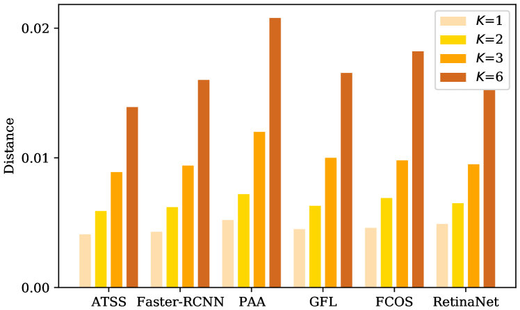
Figure 6: The distance when varying $K$ from 1 to 6.

aux head	pos queries	#epochs	AP	AP50	AP75
✗	✗	12	37.1	55.5	40.0
		36	43.3	62.3	47.1
✓	✗	12	41.6(+4.5)	59.8	45.6
		36	46.2(+2.9)	64.7	50.9
✗	✓	12	40.5(+3.4)	58.8	44.4
		36	45.3(+2.0)	63.5	49.8
✓	✓	12	42.3(+5.2)	60.5	46.1
		36	46.8(+3.5)	65.1	51.5

Table 9: “aux head” denotes training with an auxiliary head and “pos queries” means the customized positive queries generation.

Should the added heads be different? Collaborative training with two ATSS heads (49.2% AP) still improves the model with one ATSS head (48.7% AP) as ATSS is complementary to the DETR head in our analysis. Besides, introducing a diverse and complementary auxiliary head rather than the same one as the original head, e.g., Faster-RCNN, can bring better gains (49.5% AP). Note that this is not contradictory to above conclusion; instead, we can obtain the best performance with few different heads ($K\leq 2$) as the conflicts are insignificant, but we are faced with severe conflicts when using many different heads ($K>3$).

The effect of each component. We perform a component-wise ablation to thoroughly analyze the effect of each component in Table 9. Incorporating the auxiliary head yields significant gains since the dense spatial supervision enables the encoder features more discriminative. Alternatively, introducing customized positive queries also contributes remarkably to the final results, while improving the training efficiency of the one-to-one set matching. Both techniques can accelerate convergence and improve performance. In summary, we observe the overall improvements stem from more discriminative features for the encoder and more efficient attention learning for the decoder.

Method	$K$	#epochs	GPU hours	AP
Deformable-DETR	1	36	288	46.8
Deformable-DETR	0	50	333	44.5
Deformable-DETR	0	100	667	46.0
Deformable-DETR	0	150	1000	45.9

Table 10: Comparison to baselines with longer schedule.

Branch	NMS	$K=0$	$K=1$	$K=2$
Deformable-DETR++	✗	47.1	48.7(+1.6)	49.5(+2.4)
ATSS	✓	46.8	47.4(+0.6)	48.0(+1.2)
Faster-RCNN	✓	45.9	-	46.7(+0.8)

Table 11: Collaborative training consistently improves performances of all branches on Deformable-DETR++ with ResNet-50.

Comparisons to the longer training schedule. As presented in Table 10, we find Deformable-DETR can not benefit from longer training as the performance saturates. On the contrary, $\mathcal{C}$o-DETR greatly accelerates the convergence as well as increasing the peak performance.

Performance of auxiliary branches. Surprisingly, we observe $\mathcal{C}$o-DETR also brings consistent gains for auxiliary heads in Table 11. This implies our training paradigm contributes to more discriminative encoder representations, which improves the performances of both decoder and auxiliary heads.

Difference in distribution of original and customized positive queries. We visualize the positions of original positive queries and customized positive queries in Figure 7. We only show one object (green box) per image. Positive queries assigned by Hungarian Matching in the decoder are marked in red. We mark positive queries extracted from Faster-RCNN and ATSS in blue and orange, respectively. These customized queries are distributed around the center region of the instance and provide sufficient supervision signals for the detector.

Does distribution difference lead to instability? We compute the average distance between original and customized queries in Figure 7. The average distance between original negative queries and customized positive queries is significantly larger than the distance between original and customized positive queries. As this distribution gap between original and customized queries is marginal, there is no instability encountered during training.

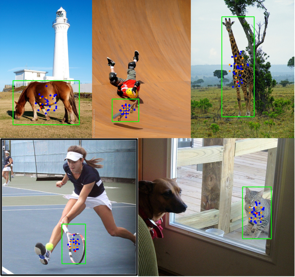
(a) Visualizations of queries.

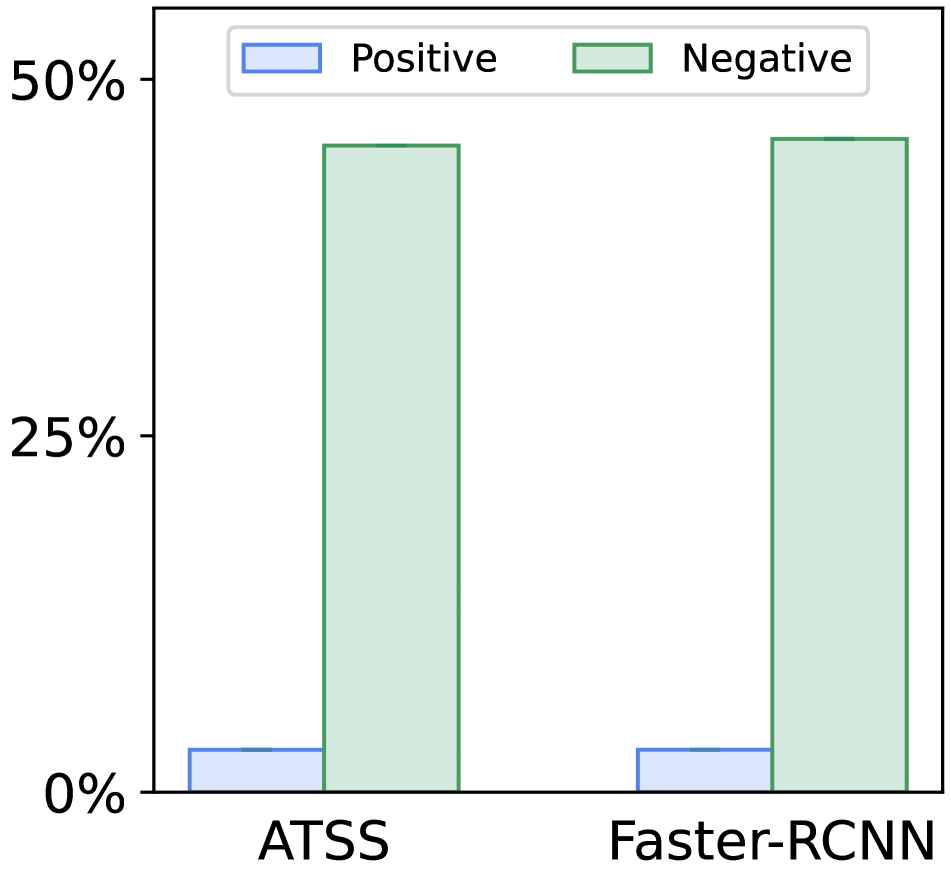
(b) Normalized distances.

Figure 7: Distribution of original and customized queries.

5 Conclusions

In this paper, we present a novel collaborative hybrid assignments training scheme, namely $\mathcal{C}$o-DETR, to learn more efficient and effective DETR-based detectors from versatile label assignment manners. This new training scheme can easily enhance the encoder’s learning ability in end-to-end detectors by training the multiple parallel auxiliary heads supervised by one-to-many label assignments. In addition, we conduct extra customized positive queries by extracting the positive coordinates from these auxiliary heads to improve the training efficiency of positive samples in decoder. Extensive experiments on COCO dataset demonstrate the efficiency and effectiveness of $\mathcal{C}$o-DETR. Surprisingly, incorporated with ViT-L backbone, we achieve 66.0% AP on COCO test-dev and 67.9% AP on LVIS val, establishing the new state-of-the-art detector with much fewer model sizes.

DETRs with Collaborative Hybrid Assignments Training
Supplementary Material

Appendix A More ablation studies

#convs	0	1	2	3	4	5
AP	41.8	42.3	41.9	42.1	42.3	42.0

Table 12: Influence of number of convolutions in auxiliary head.

$\lambda_{1}$	$\lambda_{2}$	#epochs	AP	APS	APM	APL
0.25	2.0	36	46.2	28.3	49.7	60.4
0.5	2.0	36	46.6	29.0	50.5	61.2
1.0	2.0	36	46.8	28.1	50.6	61.3
2.0	2.0	36	46.1	27.4	49.7	61.4
1.0	1.0	36	46.1	27.9	49.7	60.9
1.0	2.0	36	46.8	28.1	50.6	61.3
1.0	3.0	36	46.5	29.3	50.4	61.4
1.0	4.0	36	46.3	29.0	50.1	61.0

Table 13: Results of hyper-parameter tuning for $\lambda_{1}$ and $\lambda_{2}$.

The number of stacked convolutions. Table 12 reveals our method is robust for the number of stacked convolutions in the auxiliary head (trained for 12 epochs). Concretely, we simply choose only 1 shared convolution to enable lightweight while achieving higher performance.

Loss weights of collaborative training. Experimental results related to weighting the coefficient $\lambda_{1}$ and $\lambda_{2}$ are presented in Table 13. We find the proposed method is quite insensitive to the variations of $\{\lambda_{1},\lambda_{2}\}$, since the performance slightly fluctuates when varying the loss coefficients. In summary, the coefficients $\{\lambda_{1},\lambda_{2}\}$ are robust and we set $\{\lambda_{1},\lambda_{2}\}$ to $\{1.0,2.0\}$ by default.

Figure 8: The relation matrix for the DETR head, ATSS head, and Faster-RCNN head. The detector is $\mathcal{C}$o-Deformable-DETR ($K=2$) with ResNet-50.

Figure 9: Distances among 7 various heads in our model with $K=6$.

The number of customized positive queries. We compute the average ratio of positive samples in one-to-many label assignment to the ground-truth boxes. For instance, the ratio is 18.7 for Faster-RCNN and 8.8 for ATSS on COCO dataset, indicating more than 8$\times$ extra positive queries are introduced when $K=1$.

Effectiveness of collaborative one-to-many label assignments. To verify the effectiveness of our feature learning mechanism, we compare our approach with Group-DETR (3 groups) and $\mathcal{H}$-DETR. First, we find $\mathcal{C}$o-DETR performs better than hybrid matching scheme [16] while training faster and requiring less GPU memory in Table 6. As shown in Table 8, our method ($K=1$) achieves 46.2% AP, surpassing Group-DETR (44.6% AP) by a large margin even without the customized positive queries generation. More importantly, the IoF-IoB curve in Figure 2 demonstrates Group-DETR fails to enhance the feature representations in the encoder, while our method alleviates the poorly feature learning.

Conflicts analysis. We have defined the distance between head $H_{i}$ and head $H_{j}$, and the average distance of $H_{i}$ to measure the optimization conflicts in this study:

$$\mathcal{S}_{i,j}=\frac{1}{|\mathbf{D}|}\sum_{\mathbf{I}\in\mathbf{D}}\mathrm{KL}(\mathcal{C}(H_{i}(\mathbf{I})),\mathcal{C}(H_{j}(\mathbf{I})),$$ (11)

$$\mathcal{S}_{i}=\frac{1}{2(K-1)}\sum_{j\neq i}^{K}(\mathcal{S}_{i,j}+\mathcal{S}_{j,i}),$$ (12)

where $\mathrm{KL}$, $\mathbf{D}$, $\mathbf{I}$, $\mathcal{C}$ refer to KL divergence, dataset, the input image, and class activation maps (CAM) [29]. In our implementation, we choose the validation set COCO val as $\mathbf{D}$ and Grad-CAM as $\mathcal{C}$. We use the output features of DETR encoder to compute the CAM maps. More specifically, we show the detailed distances when $K=2$ and $K=6$ in Figure 8 and Figure 9, respetively. The larger distance metric of $\mathcal{S}_{i,j}$ indicates $H_{i}$ is less consistent to $H_{j}$ and contributes to the optimization inconsistency.

Appendix B More implementation details

One-stage auxiliary heads. Based on the conventional one-stage detectors, we experiment with various first-stage designs [41, 19, 32, 17, 21] for the auxiliary heads. First, we use the GIoU [28] loss for the one-stage heads. Then, the number of stacked convolutions is reduced from $4$ to $1$. Such modification improves the training efficiency without any accuracy drop. For anchor-free detectors, e.g., FCOS [32], we assign the width of $8\times 2^{j}$ and height of $8\times 2^{j}$ for the positive coordinates with stride $2^{j}$.

Two-stage auxiliary heads. We adopt the RPN and RCNN as our two-stage auxiliary heads based on the popular Faster-RCNN [27] and Mask-RCNN [14] detectors. To make $\mathcal{C}$o-DETR compatible with various detection heads, we adopt the same multi-scale features (stride 8 to stride 128) as the one-stage paradigm for two-stage auxiliary heads. Moreover, we adopt the GIoU loss for regression in the RCNN stage.

System-level comparison on COCO. We first initialize the ViT-L backbone with EVA-02 weights. Then we perform intermediate finetuning on the Objects365 dataset using $\mathcal{C}$o-DINO-Deformable-DETR for 26 epochs and reduce the learning rate by a factor of 0.1 at epoch 24. The initial learning rate is $2.5\times 10^{-4}$ and the batch size is 224. We choose the maximum size of input images as 1280 and randomly resize the shorter size to 480$-$1024. Moreover, we use 1500 object queries and 1000 DN queries for this model. Finally, we finetune $\mathcal{C}$o-DETR on COCO for 12 epochs with an initial learning rate of $5\times 10^{-5}$ and drop the learning rate at the 8-th epoch by multiplying 0.1. The shorter size of input images is enlarged to 480$-$1536 and the longer size is no more than 2400. We employ EMA and train this model with a batch size of 64.

System-level comparison on LVIS. In contrast to the COCO setting, we use $\mathcal{C}$o-DINO-Deformable-DETR++ to perform intermediate finetuning on the Objects365 dataset, as we find LSJ augmentation works better on the LVIS dataset. A batch size of 192, an initial learning rate of $2\times 10^{-4}$, and an input image size of 1280$\times$1280 are used. We use 900 object queries and 1000 DN queries for this model. During finetuning on LVIS, we arm it with an additional auxiliary mask branch and increase the input size to 1536$\times$1536. Besides, we train the model without EMA for 16 epochs, where the batch size is set to 64, and the initial learning rate is set to $5\times 10^{-5}$, which is reduced by a factor of 0.1 at the 9-th and 15-th epoch.

References

- [1] Nicolas Carion, Francisco Massa, Gabriel Synnaeve, Nicolas Usunier, Alexander Kirillov, and Sergey Zagoruyko. End-to-end object detection with transformers. ArXiv, abs/2005.12872, 2020.
- [2] Fangyi Chen, Han Zhang, Kai Hu, Yu-kai Huang, Chenchen Zhu, and Marios Savvides. Enhanced training of query-based object detection via selective query recollection. arXiv preprint arXiv:2212.07593, 2022.
- [3] Kai Chen, Jiangmiao Pang, Jiaqi Wang, Yu Xiong, Xiaoxiao Li, Shuyang Sun, Wansen Feng, Ziwei Liu, Jianping Shi, Wanli Ouyang, et al. Hybrid task cascade for instance segmentation. In Proceedings of the IEEE/CVF Conference on Computer Vision and Pattern Recognition, pages 4974–4983, 2019.
- [4] Kai Chen, Jiaqi Wang, Jiangmiao Pang, Yuhang Cao, Yu Xiong, Xiaoxiao Li, Shuyang Sun, Wansen Feng, Ziwei Liu, Jiarui Xu, et al. Mmdetection: Open mmlab detection toolbox and benchmark. arXiv preprint arXiv:1906.07155, 2019.
- [5] Qiang Chen, Xiaokang Chen, Gang Zeng, and Jingdong Wang. Group detr: Fast training convergence with decoupled one-to-many label assignment. arXiv preprint arXiv:2207.13085, 2022.
- [6] Qiang Chen, Jian Wang, Chuchu Han, Shan Zhang, Zexian Li, Xiaokang Chen, Jiahui Chen, Xiaodi Wang, Shuming Han, Gang Zhang, et al. Group detr v2: Strong object detector with encoder-decoder pretraining. arXiv preprint arXiv:2211.03594, 2022.
- [7] Alexey Dosovitskiy, Lucas Beyer, Alexander Kolesnikov, Dirk Weissenborn, Xiaohua Zhai, Thomas Unterthiner, Mostafa Dehghani, Matthias Minderer, Georg Heigold, Sylvain Gelly, Jakob Uszkoreit, and Neil Houlsby. An image is worth 16x16 words: Transformers for image recognition at scale. ArXiv, abs/2010.11929, 2021.
- [8] Yuxin Fang, Quan Sun, Xinggang Wang, Tiejun Huang, Xinlong Wang, and Yue Cao. Eva-02: A visual representation for neon genesis. arXiv preprint arXiv:2303.11331, 2023.
- [9] Ziteng Gao, Limin Wang, Bing Han, and Sheng Guo. Adamixer: A fast-converging query-based object detector. In Proceedings of the IEEE/CVF Conference on Computer Vision and Pattern Recognition, pages 5364–5373, 2022.
- [10] Golnaz Ghiasi, Yin Cui, Aravind Srinivas, Rui Qian, Tsung-Yi Lin, Ekin D Cubuk, Quoc V Le, and Barret Zoph. Simple copy-paste is a strong data augmentation method for instance segmentation. In Proceedings of the IEEE/CVF conference on computer vision and pattern recognition, pages 2918–2928, 2021.
- [11] Ross Girshick. Fast r-cnn. In Proceedings of the IEEE international conference on computer vision, pages 1440–1448, 2015.
- [12] Agrim Gupta, Piotr Dollar, and Ross Girshick. Lvis: A dataset for large vocabulary instance segmentation. In Proceedings of the IEEE/CVF conference on computer vision and pattern recognition, pages 5356–5364, 2019.
- [13] Kaiming He, Xinlei Chen, Saining Xie, Yanghao Li, Piotr Dollár, and Ross Girshick. Masked autoencoders are scalable vision learners. In Proceedings of the IEEE/CVF conference on computer vision and pattern recognition, pages 16000–16009, 2022.
- [14] Kaiming He, Georgia Gkioxari, Piotr Dollár, and Ross Girshick. Mask r-cnn. In Proceedings of the IEEE international conference on computer vision, pages 2961–2969, 2017.
- [15] Kaiming He, X. Zhang, Shaoqing Ren, and Jian Sun. Deep residual learning for image recognition. 2016 IEEE Conference on Computer Vision and Pattern Recognition (CVPR), pages 770–778, 2016.
- [16] Ding Jia, Yuhui Yuan, Haodi He, Xiaopei Wu, Haojun Yu, Weihong Lin, Lei Sun, Chao Zhang, and Han Hu. Detrs with hybrid matching. arXiv preprint arXiv:2207.13080, 2022.
- [17] Kang Kim and Hee Seok Lee. Probabilistic anchor assignment with iou prediction for object detection. In European Conference on Computer Vision, pages 355–371. Springer, 2020.
- [18] Feng Li, Hao Zhang, Shilong Liu, Jian Guo, Lionel M Ni, and Lei Zhang. Dn-detr: Accelerate detr training by introducing query denoising. In Proceedings of the IEEE/CVF Conference on Computer Vision and Pattern Recognition, pages 13619–13627, 2022.
- [19] Xiang Li, Wenhai Wang, Lijun Wu, Shuo Chen, Xiaolin Hu, Jun Li, Jinhui Tang, and Jian Yang. Generalized focal loss: Learning qualified and distributed bounding boxes for dense object detection. Advances in Neural Information Processing Systems, 33:21002–21012, 2020.
- [20] Yanghao Li, Hanzi Mao, Ross Girshick, and Kaiming He. Exploring plain vision transformer backbones for object detection. arXiv preprint arXiv:2203.16527, 2022.
- [21] Tsung-Yi Lin, Priya Goyal, Ross Girshick, Kaiming He, and Piotr Dollár. Focal loss for dense object detection. In Proceedings of the IEEE international conference on computer vision, pages 2980–2988, 2017.
- [22] Tsung-Yi Lin, Michael Maire, Serge Belongie, James Hays, Pietro Perona, Deva Ramanan, Piotr Dollár, and C Lawrence Zitnick. Microsoft coco: Common objects in context. In European conference on computer vision, pages 740–755. Springer, 2014.
- [23] Shilong Liu, Feng Li, Hao Zhang, Xiao Yang, Xianbiao Qi, Hang Su, Jun Zhu, and Lei Zhang. Dab-detr: Dynamic anchor boxes are better queries for detr. arXiv preprint arXiv:2201.12329, 2022.
- [24] Ze Liu, Han Hu, Yutong Lin, Zhuliang Yao, Zhenda Xie, Yixuan Wei, Jia Ning, Yue Cao, Zheng Zhang, Li Dong, et al. Swin transformer v2: Scaling up capacity and resolution. In Proceedings of the IEEE/CVF Conference on Computer Vision and Pattern Recognition, pages 12009–12019, 2022.
- [25] Ze Liu, Yutong Lin, Yue Cao, Han Hu, Yixuan Wei, Zheng Zhang, S. Lin, and B. Guo. Swin transformer: Hierarchical vision transformer using shifted windows. ArXiv, abs/2103.14030, 2021.
- [26] Depu Meng, Xiaokang Chen, Zejia Fan, Gang Zeng, Houqiang Li, Yuhui Yuan, Lei Sun, and Jingdong Wang. Conditional detr for fast training convergence. In Proceedings of the IEEE/CVF International Conference on Computer Vision, pages 3651–3660, 2021.
- [27] Shaoqing Ren, Kaiming He, Ross Girshick, and Jian Sun. Faster r-cnn: Towards real-time object detection with region proposal networks. Advances in neural information processing systems, 28, 2015.
- [28] Hamid Rezatofighi, Nathan Tsoi, JunYoung Gwak, Amir Sadeghian, Ian Reid, and Silvio Savarese. Generalized intersection over union: A metric and a loss for bounding box regression. In Proceedings of the IEEE/CVF conference on computer vision and pattern recognition, pages 658–666, 2019.
- [29] Ramprasaath R Selvaraju, Michael Cogswell, Abhishek Das, Ramakrishna Vedantam, Devi Parikh, and Dhruv Batra. Grad-cam: Visual explanations from deep networks via gradient-based localization. In Proceedings of the IEEE international conference on computer vision, pages 618–626, 2017.
- [30] Shuai Shao, Zeming Li, Tianyuan Zhang, Chao Peng, Gang Yu, Xiangyu Zhang, Jing Li, and Jian Sun. Objects365: A large-scale, high-quality dataset for object detection. In Proceedings of the IEEE/CVF international conference on computer vision, pages 8430–8439, 2019.
- [31] Guanglu Song, Yu Liu, and Xiaogang Wang. Revisiting the sibling head in object detector. In Proceedings of the IEEE/CVF conference on computer vision and pattern recognition, pages 11563–11572, 2020.
- [32] Zhi Tian, Chunhua Shen, Hao Chen, and Tong He. Fcos: Fully convolutional one-stage object detection. In Proceedings of the IEEE/CVF international conference on computer vision, pages 9627–9636, 2019.
- [33] Wenhui Wang, Hangbo Bao, Li Dong, Johan Bjorck, Zhiliang Peng, Qiang Liu, Kriti Aggarwal, Owais Khan Mohammed, Saksham Singhal, Subhojit Som, et al. Image as a foreign language: Beit pretraining for all vision and vision-language tasks. arXiv preprint arXiv:2208.10442, 2022.
- [34] Wenhai Wang, Jifeng Dai, and Zhe Chen. Internimage: Exploring large-scale vision foundation models with deformable convolutions. arXiv preprint arXiv:2211.05778, 2022.
- [35] Yingming Wang, Xiangyu Zhang, Tong Yang, and Jian Sun. Anchor detr: Query design for transformer-based detector. In Proceedings of the AAAI conference on artificial intelligence, volume 36, pages 2567–2575, 2022.
- [36] Yixuan Wei, Han Hu, Zhenda Xie, Zheng Zhang, Yue Cao, Jianmin Bao, Dong Chen, and Baining Guo. Contrastive learning rivals masked image modeling in fine-tuning via feature distillation. arXiv preprint arXiv:2205.14141, 2022.
- [37] Zeyue Xue, Jianming Liang, Guanglu Song, Zhuofan Zong, Liang Chen, Yu Liu, and Ping Luo. Large-batch optimization for dense visual predictions. In Advances in Neural Information Processing Systems, 2022.
- [38] Jianwei Yang, Chunyuan Li, and Jianfeng Gao. Focal modulation networks. arXiv preprint arXiv:2203.11926, 2022.
- [39] Hao Zhang, Feng Li, Shilong Liu, Lei Zhang, Hang Su, Jun Zhu, Lionel M Ni, and Heung-Yeung Shum. Dino: Detr with improved denoising anchor boxes for end-to-end object detection. arXiv preprint arXiv:2203.03605, 2022.
- [40] Haotian Zhang, Pengchuan Zhang, Xiaowei Hu, Yen-Chun Chen, Liunian Li, Xiyang Dai, Lijuan Wang, Lu Yuan, Jenq-Neng Hwang, and Jianfeng Gao. Glipv2: Unifying localization and vision-language understanding. Advances in Neural Information Processing Systems, 35:36067–36080, 2022.
- [41] Shifeng Zhang, Cheng Chi, Yongqiang Yao, Zhen Lei, and Stan Z Li. Bridging the gap between anchor-based and anchor-free detection via adaptive training sample selection. In Proceedings of the IEEE/CVF conference on computer vision and pattern recognition, pages 9759–9768, 2020.
- [42] Xingyi Zhou, Vladlen Koltun, and Philipp Krähenbühl. Probabilistic two-stage detection. arXiv preprint arXiv:2103.07461, 2021.
- [43] Xizhou Zhu, Weijie Su, Lewei Lu, Bin Li, Xiaogang Wang, and Jifeng Dai. Deformable detr: Deformable transformers for end-to-end object detection. arXiv preprint arXiv:2010.04159, 2020.
- [44] Zhuofan Zong, Qianggang Cao, and Biao Leng. Rcnet: Reverse feature pyramid and cross-scale shift network for object detection. In Proceedings of the 29th ACM International Conference on Multimedia, pages 5637–5645, 2021.