SketchBoost: Fast Gradient Boosted Decision Tree for Multioutput Problems

Abstract

Gradient Boosted Decision Tree (GBDT) is a widely-used machine learning algorithm that has been shown to achieve state-of-the-art results on many standard data science problems. We are interested in its application to multioutput problems when the output is highly multidimensional. Although there are highly effective GBDT implementations, their scalability to such problems is still unsatisfactory. In this paper, we propose novel methods aiming to accelerate the training process of GBDT in the multioutput scenario. The idea behind these methods lies in the approximate computation of a scoring function used to find the best split of decision trees. These methods are implemented in SketchBoost, which itself is integrated into our easily customizable Python-based GPU implementation of GBDT called Py-Boost. Our numerical study demonstrates that SketchBoost speeds up the training process of GBDT by up to over $40$ times while achieving comparable or even better performance.

1 Introduction

Gradient Boosted Decision Tree (GBDT) is one of the most powerful methods for solving prediction problems in both classification and regression domains. It is a dominant tool today in application domains where tabular data is abundant, for example, in e-commerce, financial, and retail industries. GBDT has contributed to a large amount of top solutions in benchmark competitions such as Kaggle. This makes GBDT a fundamental component in the modern data scientist’s toolkit.

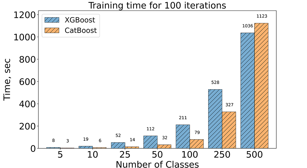
Figure 1: Training time of XGBoost and CatBoost for different number of classes on a synthetic dataset for multiclass classification. Synthetic dataset contains $2000$k instances, each described by $100$ features. The maximal tree depth was limited to $6$. The experiment was conducted on GPU. Further details are given in Section B.7.

The main focus of this paper is the scalability of GBDT to multioutput problems. Such problems include multiclass classification (a classification task with more than two mutually exclusive classes), multilabel classification (a classification task with more than two classes that are not mutually exclusive), and multioutput regression (a regression task with a multivariate response variable). These problems arise in various areas such as Finance (Obermann and Waack, 2016), Multivariate Time Series Forecasting (Zhai, Yao, and Zhou, 2020), Recommender Systems (Jahrer, Töscher, and Legenstein, 2010), and others.

There are several extremely efficient, open-source, and production-ready implementations of gradient boosting such as XGBoost (Chen and Guestrin, 2016), LightGBM (Ke, Meng, Finley, Wang, Chen, Ma, Ye, and Liu, 2017), and CatBoost (Prokhorenkova, Gusev, Vorobev, Dorogush, and Gulin, 2018). Even for them, learning a GBDT model for moderately large datasets can require much time. Furthermore, this time also grows with the output size of a model. Figure 1 demonstrates how rapidly the training time of XGBoost and CatBoost grows with the output dimension. Consequently, the number of possible applications of GBDT in the multioutput regime is very limited.

GBDT is a boosting-based algorithm that ensembles decision trees as “base learners”. At each boosting step, a newly added tree improves the ensemble by minimizing the error of an already built composition. There are two possible strategies on how to use GBDT to handle a multioutput problem.

• One-versus-all strategy. Here, at each boosting step, a single decision tree is built for every output. Consequently, every output is handled separately. XGBoost and LightGBM use this strategy.

• Single-tree strategy. Here, at each boosting step, a single multivariate decision tree is built for all outputs. Consequently, all outputs are handled together. CatBoost uses this strategy.

The computational complexity of both strategies is proportional to the number of outputs. Specifically, the one-versus-all strategy requires fitting a separate decision tree for each single output at each boosting step. The single-tree strategy requires scanning all the output dimensions (a) to estimate the information gain during the search of the best tree structure and (b) to compute leaf values of a decision tree with a given structure (see details in Section 2). A straightforward idea to reduce the training time of single-tree GBDT is to exclude some of the outputs during the search of the tree structure which is the most time-consuming step of GBDT. However, this turns out to be rather challenging since it is unclear what outputs contribute the most to the information gain. In this paper, we address this problem and propose novel methods for fast scoring of multivariate decision trees which show a significant decrease in computational overhead without compromising the performance of the final model.

Related work.

Many suggestions have been made to speed up the training process of GBDT. Some methods reduce the number of data instances used to train each base learner. For example, Stochastic Gradient Boosting (SGB) (Friedman, 2002) chooses a random subset of data instances, gradient-based one-side sampling (GOSS) (Ke et al., 2017) keeps the instances with large gradients and randomly drops the instances with small gradients, and Minimal Variance Sampling (MVS) (Ibragimov and Gusev, 2019) randomly chooses the instances to maximize the estimation accuracy of split scoring. Similarly, some methods reduce the number of features. For example, one can choose a random subset of features or use principal component analysis or projection pursuit to exclude weak features; see (Jimenez and Landgrebe, 1999; Zhou, 2012; Appel et al., 2013). LightGBM (Ke et al., 2017) uses exclusive feature bundling (EFB) where sparse features are greedily bundled together. CatBoost (Prokhorenkova et al., 2018) replaces categorical features with numerical ones using a special algorithm based on target statistics. Finally, some methods reduce the number of split candidates during the split scoring. The pre-sorted algorithm (Mehta et al., 1996) enumerates all possible split points on the pre-sorted feature values. The histogram-based algorithm (Alsabti et al., 1998; Jin and Agrawal, 2003b; Li et al., 2007) buckets continuous feature values into discrete bins and uses these bins to construct feature histograms.

Regarding the multioutput regime, the existing methods to accelerate the training process of GBDT naturally fall into the following two categories: problem transformation and algorithm adaptation. Transformation methods (see, for example, (Hsu et al., 2009; Tai and Lin, 2012; Kapoor et al., 2012; Cissé et al., 2012; Wicker et al., 2016)) reduce the number of targets before training a model. They mainly differ in the choice of compression and decompression techniques and significantly rely on the problem structure or data assumptions. These methods pay a price in terms of prediction accuracy due to the loss of information during the compression phase, and as a result, they do not consistently outperform the full baseline. Adaptation methods directly extend some specific algorithms to efficiently solve multioutput problems. To the best of our knowledge, there are only two algorithm adaptation works for GBDT. Namely, Si et al. (2017) and Zhang and Jung (2021) consider models with sparse output and discuss how to utilize this sparsity to enforce the leaf values to be also sparse. Their modifications of GBDT are called GBDT-Sparse and GBDT-MO (sparse).

We approach the problem of fast GBDT training in the multioutput regime from a different perspective. Namely, instead of employing the model sparsity, we, loosely speaking, approximate the scoring function used to find the best tree structure using the most essential outputs while keeping other boosting steps without change. The methods we suggest are completely different from the ones mentioned above and can be applied to models with both dense and sparse outputs. Moreover, our methods can be easily combined with transformation methods (by compressing the outputs beforehand and decompressing predictions afterward) or the sparsity utilization as in GBDT-Sparse and GBDT-MO (by computing the optimal leaf values with sparsity constraint as in these algorithms).

Contributions.

The contributions of this work can be summarized as follows.

• We propose and theoretically justify three novel methods to speed up GBDT on multioutput tasks. These methods are generic, they can be used with any loss function and do not rely on any specific data assumptions (for example, sparsity or class hierarchy) or the problem structure (for example, multilabel or multiclass). Moreover, they do not drop down the model quality and can be easily integrated into any GBDT realization that uses the single-tree strategy.

• We implemented the proposed methods in SketchBoost. SketchBoost itself is a part of our Python-based implementation of GBDT called Py-Boost. This implementation seems to be of independent interest since it does not use low-level programming languages and is easily customizable. Although it is written in Python, it is fast since it works on GPU.

• We present an empirical study using public datasets which demonstrates that SketchBoost achieves comparable or even better performance compared to the existing state-of-the-art boosting toolkits but in remarkably less time.

Paper Organization.

First, we review the GBDT algorithm in Section 2. Next, we propose methods leading to a noticeable reduction in the training time of GBDT on multioutput tasks in Section 3. We illustrate the performance of these methods on real-world datasets in Section 4. Proofs and experiment details are postponed to Appendix A and Appendix B.

2 Preliminaries

Let $\{(x_{i},y_{i})\}_{i=1}^{n}$ be a dataset with $n$ samples, where $x_{i}\in\mathbb{R}^{m}$ is an $m$ dimensional input and $y_{i}\in\mathbb{R}^{d}$ is a $d$ dimensional output. Let also $\mathcal{F}$ be a class of base learners, that is, functions $f:\mathbb{R}^{m}\to\mathbb{R}^{d}$. In Gradient Boosting, the idea of which goes back to Schapire (1990), Freund (1995), Freund and Schapire (1997), the model $F_{T}$ uses $T\in\mathbb{N}$ base learners $f\in\mathcal{F}$ and is trained in an additive and greedy manner. Namely, at the $t$-th iteration, a newly added base learner $f$ improves the quality of an already built model $F_{t-1}$ by minimization of some specified loss function $l:\mathbb{R}^{d}\times\mathbb{R}^{d}\to\mathbb{R}$,

$$\mathcal{L}_{t}(f)=\sum\nolimits_{i=1}^{n}l(y_{i},F_{t-1}(x_{i})+f(x_{i})).$$

This optimization problem is usually approached by the Newton method using the second-order approximation of the loss function

$$f^{*}_{t}\in\operatornamewithlimits{argmin}_{f\in\mathcal{F}}\Biggl{\{}\sum_{i=1}^{n}\Bigl{(}g_{i}^{\top}f(x_{i})+\frac{1}{2}\bigl{(}f(x_{i})\bigr{)}^{\top}H_{i}f(x_{i})\Bigr{)}+\Omega(f)\Biggr{\}},$$ (1)

where we omitted a term independent of $f$; here $\Omega(f)$ is a regularization term, usually added to build non-complex models, and Due to the complexity of optimization over a large set of base learners $\mathcal{F}$, the problem (1) is solved typically in a greedy fashion which leads us to an approximate minimizer $f_{t}$. Finally, the model $F_{t}$ is updated by applying a learning rate $\varepsilon>0$ typically treated as a hyperparameter: $F_{t}=F_{t-1}+\varepsilon f_{t}.$

GBDT uses decision trees as the base learners $\mathcal{F}$; see the seminal paper of Friedman (2001). A decision tree is a model built by a recursive partition of the feature space into several disjoint regions. Each final leaf is assigned to a value, which is a response of the tree in the given region. Based on this construction mechanism, a decision tree $f$ can be expressed as

$$f(x)=\sum\nolimits_{j=1}^{J}v_{j}\cdot[x\in R_{j}],$$

where $[\text{predicate}]$ denotes the indicator function, $J$ is the number of leaves, $R_{j}$ is the $j$-th leaf, and $v_{j}\in\mathbb{R}^{d}$ is the value of $j$-th leaf. The problem of learning $f_{t}$ can be naturally divided into two separate problems: (1) finding the best tree structure (dividing the feature space into $J$ areas $R_{1},\ldots,R_{J}$), and (2) fitting a decision tree with a given structure (computing leaf values $v_{1},\ldots,v_{J}$).

Finding the leaf values.

Since decision trees take constant values at each leaf, for a decision tree $f_{t}$ with leaves $R_{1},\ldots,R_{J}$, we can optimize the objective function from (1) for each leaf $R_{j}$ separately,

$$v_{j} =\operatornamewithlimits{argmin}_{v\in\mathbb{R}^{d}}\Biggl{\{}\sum_{x_{i}\in R_{j}}\Bigl{(}g_{i}^{\top}v+\frac{1}{2}v^{\top}H_{i}v\Bigr{)}+\frac{\lambda}{2}\|v\|^{2}\Biggr{\}}=-\Biggl{(}\sum_{x_{i}\in R_{j}}H_{i}+\lambda I\Biggr{)}^{-1}\Biggl{(}\sum_{x_{i}\in R_{j}}g_{i}\Biggr{)},$$

where we employ $l_{2}$ regularization on leaf values with a parameter $\lambda>0$; here $I$ denotes the identity matrix and $\|\cdot\|$ denotes the Euclidean norm.

It is worth mentioning that if the loss function $l$ is separable with respect to different outputs, all Hessians $H_{1},\ldots,H_{n}$ are diagonal. If it is not the case, it is a common practice to purposely simplify them to this extent in order to avoid time-consuming matrix inversion. It is done so in most of the single-tree GBDT algorithms (for example, CatBoost, GBDT-Sparse, and GBDT-MO). We will also follow this idea in our work. For diagonal Hessians, the optimal leaf values can be rewritten as

$$v_{j}=-\frac{\sum_{i\in R}g_{i}^{j}}{\sum_{i\in R}h_{i}^{j}+\lambda},\quad\text{where }\,g_{i}=\begin{pmatrix}g_{i}^{1}\\ \vdots\\ g_{i}^{d}\end{pmatrix}\,\text{ and }\,H_{i}=\begin{pmatrix}h_{i}^{1}&\ldots&0\\ \vdots&\ddots&\vdots\\ 0&\ldots&h_{i}^{d}\end{pmatrix}.$$ (6)

Finding the tree structure.

Substituting the leaf values from (6) back into the objective function, and omitting insignificant terms, we obtain

$$\operatorname{Loss}(f_{t})=-\frac{1}{2}\sum_{j=1}^{J}S(R_{j}),\quad\text{where}\quad S(R)=\sum_{j=1}^{d}\frac{\bigl{(}\sum_{x_{i}\in R}g_{i}^{j}\bigr{)}^{2}}{\sum_{x_{i}\in R}h_{i}^{j}+\lambda}.$$ (7)

The function $S(\cdot)$ will be referred to as the scoring function. To find the best tree structure, we use a greedy algorithm that starts from a single leaf and iteratively adds branches to the tree. At a general step, we want to split one of existing leaves. To do this, we iterate through all leaves, features, and thresholds for each feature (they are usually determined by the histogram-based algorithm). For all leaves $R$ and all possible splits for $R$, say $R_{\text{left}}$ and $R_{\text{right}}$, we compute the impurity score given by $S(R_{\text{left}})+S(R_{\text{right}}).$ The best split is considered the one which achieves the largest impurity score. This is equivalent to maximization of the information gain which is usually defined as the difference between values of the loss function before and after the split, that is,

$$\text{Gain}=-0.5\Bigl{(}S(R)-\bigl{(}S(R_{\text{left}})+S(R_{\text{right}})\bigr{)}\Bigr{)}.$$

Similar to the previous step, some simplifications can be made to speed up computation of the scoring function which is done a tremendous number of times. For instance, GBDT-Sparse does not use the second-order information at all (Hessians are simplified to identity matrices). In the multioutput regime of CatBoost, the second-order derivatives are left out during the split search and are used only to compute leaf values. GBDT-MO uses the second-order derivatives in both steps but it increases the computational complexity twice (histograms for both gradients and Hessians need to be accumulated).

3 Sketched Split Scoring

In this section, we propose three novel methods to speed up the split search for multivariate decision trees. These methods can achieve a good balance between reducing the computational complexity in the output dimension and keeping the accuracy for learned decision trees. They are generic and can be used together with the methods mentioned in the Related work section that aim at reducing the number of sample instances, features, or split candidates. Moreover, the proposed methods are easy to implement upon modern boosting frameworks such as XGBoost, LightGBM, and CatBoost.

As it was mentioned before, there are two “best practices” to speed up the training of a GBDT model on multioutput tasks: (a) to totally ignore the second-order derivatives during the split search and (b) to use only the main diagonal of the second-order derivatives to compute the leaf values. It is done so, for example, in CatBoost, one of the few boosting toolkits that use the single-tree strategy and achieve state-of-the-art results on multioutput problems. We will also develop our work on this basis.

The proposed methods are applied at each boosting step before the search for the best tree structure and after first- and second-order derivatives (see (LABEL:eq:derivatives)) are computed. The key idea of the proposed methods is to reduce the number of gradient values used in the split search so that the scoring function $S$ from (7) or, equivalently, the information gain will not change much. Specifically, the scoring function without the second-order information can be rewritten as

$$S_{G}(R)=\frac{\bigl{\|}G^{\top}v_{R}\bigr{\|}^{2}}{|R|+\lambda},\quad\text{where}\ \,G=\begin{pmatrix}g_{1}^{1}&g_{1}^{2}&\ldots&g_{1}^{d}\\ \vdots&\vdots&\ddots&\vdots\\ g_{n}^{1}&g_{n}^{2}&\ldots&g_{n}^{d}\\ \end{pmatrix}\ \,\text{and}\ \,v_{R}=\begin{pmatrix}[x_{1}\in R]\\ \vdots\\ [x_{n}\in R]\\ \end{pmatrix}.$$

Here $G\in\mathbb{R}^{n\times d}$ is the gradient matrix and $v_{R}$ is the indicator vector of the leaf $R$ (its $i$-th coordinate is equal to $1$ if $x_{i}\in R$ and $0$ otherwise). Note that we added the subscript to $S$ to indicate its dependence on the gradient matrix $G$. To reduce the complexity of computing $S_{G}$ in $d$, we approximate it with $S_{G_{k}}$ for some other matrix $G_{k}\in\mathbb{R}^{n\times k}$ with $k\ll d$. We will refer to $G_{k}$ as the sketch matrix and to $k$ as the reduced dimension or sketching dimension. We emphasize that $G_{k}$ is assumed to be used only in building histograms and finding the tree structure. After this, the optimal leaf values of a tree are assumed to be computed fairly using the full gradient matrix $G$.

Further we discuss three novel methods to construct reasonably good sketches $G_{k}$ — Top Outputs, Random Sampling, and Random Projections. These methods are motivated by the minimization of the approximation error given by

$$\operatorname{Error}(S_{G},S_{G_{k}})=\sup\nolimits_{R}\bigl{|}S_{G}(R)-S_{G_{k}}(R)\bigr{|}.$$

Here the supremum is taken over all possible leaves $R$. The reason for this choice is that we want the proposed approximation to be universal and uniformly accurate for all splits we will possibly iterate over. In Appendix A, we show that the proposed methods lead to a nearly-optimal upper bounds on the proposed error. Since the corresponding optimization problem is an instance of Integer Programming problem, methods leading to the optimal upper bounds can be obtained only by brute force, which is not an option in our case. For further details see Appendix A.

3.1 Top Outputs

The key idea of Top Outputs is rather straightforward: to choose the columns of $G$ with the largest Euclidian norm. Namely, by a slight abuse of notation, let us denote the columns of $G$ by $g_{1},\ldots,g_{d}$. Let also $i_{1},\ldots,i_{d}$ be the indexes which sort the columns of $G$ in descending order by their norm, that is, $\|g_{i_{1}}\|\geq\|g_{i_{2}}\|\geq\ldots\geq\|g_{i_{d}}\|$. Now the full gradient matrix and its sketch can be written as

$$G=\begin{pmatrix}|&|&&|\\ g_{1}&g_{2}&\ldots&g_{d}\\ |&|&&|\\ \end{pmatrix}\quad\text{and}\quad G_{k}=\begin{pmatrix}|&|&&|\\ g_{i_{1}}&g_{i_{2}}&\ldots&g_{i_{k}}\\ |&|&&|\\ \end{pmatrix}.$$

The parameter $k$ here can be chosen adaptively to the norms of $g_{1},\ldots,g_{d}$. We have not considered this generalization here since, in our view, it will greatly complicate the algorithm. Moreover, the adaptive choice of $k$ may result in large values for this parameter and hence less gain in training time.

It is worth pointing out that Top Outputs is akin to the Gradient-based One-Side Sampling (GOSS), which is successively used in LightGBM; see (Ke et al., 2017). In GOSS, data instances with small gradients are excluded to speed up the split search. Similarly, Top Outputs excludes output components with small gradient values.

This method has one major drawback. This method chooses top $k$ output dimensions which may not vary much from step to step. For instance, if several columns have large norms and others have medium norms, Top Outputs may completely ignore the latter columns during the split search. Below we consider another method that deals with this problem by introducing the randomness in the choice of output dimensions.

3.2 Random Sampling

The probabilistic approach for algebraic computations, sometimes called the “Monte-Carlo method”, is ubiquitous; we refer the reader to the monographs of Robert and Casella (2005),Mahoney (2011), and Woodruff (2014). Here we consider its application to the fast split search.

The key idea of Random Sampling is to randomly sample the columns of $G$ with probabilities proportional to their norms. Namely, we define the sampling probabilities by

$$p_{i}=\|g_{i}\|^{2}\Big{/}\sum\nolimits_{j=1}^{d}\|g_{j}\|^{2},\quad i=1,\ldots,d.$$

These probabilities are known to be optimal for random sampling since they minimize the variance of the resulting estimate; see, for example, (Robert and Casella, 2005). Further, let ${i}_{1},\ldots,{i}_{k}$ be independent and identically distributed random variables taking values $j$ with probabilities $p_{j}$, $j=1,\ldots,k$. These random variables represent indexes of the chosen columns of $G$. Finally, we consider the following sketch

$$G_{k}=\begin{pmatrix}|&|&&|\\ \overline{g}_{i_{1}}&\overline{g}_{i_{2}}&\ldots&\overline{g}_{i_{k}}\\ |&|&&|\end{pmatrix},\quad\text{where}\quad\overline{g}_{i}=\frac{1}{\sqrt{kp_{i}}}\,g_{i}.$$

The additional column normalization by $1/\sqrt{kp_{i}}$ is needed for unbiasedness of the resulting estimate.

There is a close affinity between Importance Sampling and Minimal Variance Sampling (MVS) of Ibragimov and Gusev (2019). MVS decreases the number of sample instances in the split search by maximizing the estimation accuracy of split scoring. Our idea is the same with the only difference that it is applied to output dimensions rather than sample instances.

Random Sampling works well especially in the extreme cases as those mentioned above. For example, if several outputs have large weights and others have medium weights, Random Sampling will not ignore the latter outputs due to randomness. Or, if the number of outputs with large weights is larger than $k$, Random Sampling will choose different output dimensions at different steps. As a result, the corresponding base learners will also be quite different, which usually leads to a better generalization ability of the ensemble; see Breiman (1996).

3.3 Random Projections

In the previous section, the sketch $G_{k}$ was constructed by sampling columns from $G$ according to some probability distribution. This process can be viewed as multiplication of $G$ by a matrix $\Pi$, $G_{k}=G\Pi,$ where $\Pi\in\mathbb{R}^{d\times k}$ has independent columns, and each column is all zero except for a $1$ in a random location. In Random Projections, we consider sampling matrices $\Pi$, every entry of which is an independently sampled random variable. This results in using random linear combinations of columns of $G$ as columns of $G_{k}$.

This approach is based on the Johnson-Lindenstrauss (JL) lemma; see the seminal paper of Johnson and Lindenstrauss (1984). They showed that projections $\Pi$ from $d$ dimensions onto a randomly chosen $k$-dimensional subspace do not distort the pairwise distances too much. Indyk and Motwani (1998) proved that to obtain the same guarantee, one can independently sample every entry of $\Pi$ using the normal distribution. In fact, this is true for many other distributions; see, for example, Achlioptas (2003). Since there was no significant difference between distributions in our numerical experiments, we decided to focus on the normal distribution.

In Random Projections, we consider the following sketch

$$G_{k}=G\Pi,$$

where $\Pi\in\mathbb{R}^{d\times k}$ is a random matrix filled with independently sampled $\mathcal{N}(0,k^{-1})$ entries. In Appendix A, we discuss why this choice leads to a nearly-optimal solution to the problem we consider and why the property of preserving the pairwise distances matters here.

Random Projections has the same merits as Random Sampling since it is also a random approach. Besides that, the sketch matrix $G_{k}$ here uses gradient information from all outputs since each column of $G_{k}$ is a linear combination of columns of $G$.

3.4 Complexity analysis.

Most of the GBDT frameworks use histogram-based algorithm to speed up split finding; see (Alsabti, Ranka, and Singh, 1998), (Jin and Agrawal, 2003a), and (Li, Wu, and Burges, 2008). Instead of finding the split points on all possible feature values, histogram-based algorithm buckets feature values into discrete bins and uses these bins to construct feature histograms during training. Let us say that the number of possible splits per feature is limited to $h\ll n$ (usually $h\leq 256$ to store the histogram bin index using a single byte). It is shown in (Ke et al., 2017) that in the case of a single output, splitting a leaf $R$ with $n_{R}$ samples requires $O(mn_{R})$ operations for histogram building and $O(hm)$ operations for split finding. As a result, if the actual tree construction is performed using a depth-first-search algorithm, the complexity of building a complete tree of depth $D$ is $O(Dnm+2^{D}hm)$. In the multioutput scenario, this complexity increases by $d$ times: splitting a leaf $R$ with $n_{R}$ samples costs $O(mn_{R}d+hmd)$ and depth-wise tree construction costs $O(Dmnd+2^{D}hmd)$. The methods we propose reduce the impact of $d$ to $k$ with $k\ll d$. They require a preprocessing step which can be done, depending on the method, in $O(ndk)$ or $O(nd)$ operations. As a result, the complexity of building a complete tree of depth $D$ using the depth-first search can be reduced from $O(Dmnd+2^{D}hmd)$ to $O(nd+Dmnk+2^{D}hmk)$. Taking into account that $n$, $m$, and $d$ can be extremely large, these methods may lead to a significant improvement in the training time.

4 Numerical Experiments

In this section, we numerically compare (a) the proposed methods from Section 3 to speed up GBDT in the multioutput regime and (b) existing state-of-art boosting toolkits supporting multioutput tasks.

Data.

The experiments are conducted on $9$ real-world publicly available datasets from Kaggle, OpenML, and Mulan for multiclass ($4$ datasets) and multilabel ($3$ datasets) classification and multitask regression ($2$ datasets). The associated details are given in Table 5 in Appendix B.

Py-Boost.

We implemented a simple and fast GBDT toolkit called Py-Boost. It is written in Python and hence is easily customizable. Py-Boost works only on GPU and uses Python GPU libraries such as CuPy and Numba. It follows the classic scheme described in (Chen and Guestrin, 2016); further details are provided in Section B.1. Py-Boost is available on GitHub.

SketchBoost.

SketchBoost is a part of Py-Boost library which implements the following three sketching strategies for fast split search: Top Outputs (Section 3.1), Random Sampling (Section 3.2), and Random Projections (Section 3.3). For convenience, Py-Boost without any sketching strategy is referred to as SketchBoost Full. All the following experimental results and evaluation code are also available on GitHub.

Baselines.

Primarily we compare SketchBoost with XGBoost (v1.6.0) and CatBoost (v1.0.5). There are two reasons why we have chosen these GBDT frameworks. First, they are commonly used among practitioners and represent two different approaches to multiouput tasks (one-vs-all and single-tree). Second, they can be efficiently trained on GPU, which allows us to compare their training time with GPU-based SketchBoost (with an exception for CatBoost which supports multilabel classification and multioutput regression tasks only on CPU). The reason why we have not considered LightGBM as a baseline is that it uses the same multiouput strategy as XGBoost (one-vs-all) and its latest version (v3.3.2) does not support multilabel classification and multioutput regression tasks without external wrappers. Further, we also compare SketchBoost with TabNet (v3.1.1), a popular deep learning model for tabular data; see (Arik and Pfister, 2021). Our aim here is not to make an exhaustive comparison with existing deep learning approaches (it deserves its own investigation), but to make a comparison with a different in nature approach which moreover often has satisfactory complexity on large multioutput datasets.

Experiment Design.

If there is no official train/test split, we randomly split the data into training and test sets with ratio $80\%$-$20\%$. Then each algorithm is trained with 5-fold cross-validation (the train folds are used to fit a model and the validation fold is used for early stopping). We evaluate all the obtained models on the test set and get $5$ scores for each model. The overall performance of algorithms is computed as an average score. As a performance measure, we use the cross-entropy for classification and RMSE for regression, but, for the sake of completeness, we also report the accuracy score for classification and R-squared score for regression in Section B.5. For XGBoost, Catboost, and TabNet, we do the hyperparameter optimization using the Optuna framework (Akiba, Sano, Yanase, Ohta, and Koyama, 2019). For SketchBoost, we use the same hyperparameters as for CatBoost (to speed up the experiment; we do not expect that hyperparameters will vary much since we use the same single-tree approach). The sketch size $k$ is iterated through the grid $\{1,2,5,10,20\}$ (or through a subset of this grid with values less than the output dimension). Further information on experiment design is given in Sections B.2, B.3 and B.4.

Table 1: Test errors (cross-entropy for classification and RMSE for regression) $\pm$ their standard deviation.

	SketchBoost				Baseline
Dataset	Top Outputs	Random Sampling	Random Projection	SketchBoost Full	CatBoost	XGBoost	TabNet
	(for the best $k$)	(for the best $k$)	(for the best $k$)	(multioutput)	(multioutput)	(one-vs-all)	(multioutput)
Multiclass classification
Otto (9 classes)	0.4715	0.4636	0.4566	0.4697	0.4658	0.4599	0.5363
	$\pm$0.0035	$\pm$0.0026	$\pm$0.0023	$\pm$0.0030	$\pm$0.0033	$\pm$0.0028	$\pm$0.0063
SF-Crime (39 classes)	2.2070	2.2037	2.2038	2.2067	2.2036	2.2208	2.4819
	$\pm$0.0005	$\pm$0.0004	$\pm$0.0004	$\pm$0.0003	$\pm$0.0005	$\pm$0.0008	$\pm$0.0199
Helena (100 classes)	2.5923	2.5693	2.5673	2.5865	2.5698	2.5889	2.7197
	$\pm$0.0024	$\pm$0.0022	$\pm$0.0026	$\pm$0.0025	$\pm$0.0025	$\pm$0.0032	$\pm$0.0235
Dionis (355 classes)	0.3146	0.3040	0.2848	0.3114	0.3085	0.3502	0.4753
	$\pm$0.0011	$\pm$0.0014	$\pm$0.0012	$\pm$0.0009	$\pm$0.0010	$\pm$0.0020	$\pm$0.0126
Multilabel classification
Mediamill (101 labels)	0.0745	0.0745	0.0743	0.0747	0.0754	0.0758	0.0859
	$\pm$1.3e-04	$\pm$1.3e-04	$\pm$1.1e-04	$\pm$1.3e-04	$\pm$1.1e-04	$\pm$1.1e-04	$\pm$3.3e-03
MoA (206 labels)	0.0163	0.0160	0.0160	0.0160	0.0161	0.0166	0.0193
	$\pm$2.2e-05	$\pm$1.0e-05	$\pm$6.0e-06	$\pm$9.0e-06	$\pm$2.6e-05	$\pm$2.1e-05	$\pm$3.0e-04
Delicious (983 labels)	0.0622	0.0619	0.0620	0.0619	0.0614	0.0620	0.0664
	$\pm$6.2e-05	$\pm$5.9e-05	$\pm$6.2e-05	$\pm$5.5e-05	$\pm$5.2e-05	$\pm$3.3e-05	$\pm$8.0e-04
Multitask regression
RF1 (8 tasks)	1.1860	0.9944	0.9056	1.1687	0.8975	0.9250	3.7948
	$\pm$0.1366	$\pm$0.1015	$\pm$0.0582	$\pm$0.0835	$\pm$0.0384	$\pm$0.0307	$\pm$1.5935
SCM20D (16 tasks)	88.7442	86.2964	85.8061	91.0142	90.9814	89.1045	87.3655
	$\pm$0.6346	$\pm$0.4398	$\pm$0.5534	$\pm$0.3397	$\pm$0.3652	$\pm$0.4950	$\pm$1.3316

Table 2: Training time per fold in seconds. (CatBoost does not support multilabel classification and multioutput regression tasks in the GPU mode.)

	SketchBoost (GPU)				Baseline (CPU/GPU)
Dataset	Top Outputs	Random Sampling	Random Projection	SketchBoost Full	CatBoost	XGBoost	TabNet
	(for the best $k$)	(for the best $k$)	(for the best $k$)	(multioutput)	(multioutput)	(one-vs-all)	(multioutput)
Multiclass classification					GPU	GPU	GPU
Otto (9 classes)	113	102	89	131	73	1244	903
SF-Crime (39 classes)	705	676	612	1146	659	4016	2683
Helena (100 classes)	154	180	113	355	436	1036	1196
Dionis (355 classes)	1889	2038	419	23919	18600	18635	1853
Multilabel classification					CPU	GPU	GPU
Mediamill (101 labels)	251	263	294	1777	10164	2074	1231
MoA (206 labels)	103	189	87	696	9398	376	672
Delicious (983 labels)	575	664	1259	19553	20120	15795	2902
Multitask regression					CPU	GPU	GPU
RF1 (8 tasks)	369	396	340	413	804	315	207
SCM20D (16 tasks)	499	528	479	597	798	1432	296

Results.

The final test errors are summarized in Table 1. Experiments show that, in general, SketchBoost with a sketching strategy obtains results comparable to or even better than the competing boosting frameworks. Promisingly, there is always a sketching strategy that outperforms SketchBoost Full. Random Projection achieves the best scores, but Random Sampling also performs quite well. The deterministic Top Outputs strategy scores less than other baselines everywhere. In addition, it is noticeable that the one-vs-all strategy implemented in XGBoost leads to a worse generalization ability than the single-tree strategy on most datasets.

The dependence of test scores on the sketch size $k$ for four datasets is shown in Section 4; for other datasets see Section B.5 in Appendix B. It confirms the idea that, in general, the larger values $k$ we take, the better performance we obtain. Moreover, our numerical study shows that there is a wide range of values of $k$ for which sketching strategies work well; see the detailed results for all $k$ in Table 10 and Table 11 in Appendix B. For most datasets, $k\leq 10$ is enough to obtain a result similar to or even better than SketchBoost Full or other baselines. Loosely speaking, an intuitive explanation of why reducing the output dimension may increase the ensemble quality is that building a tree using all outputs often leads to bad split choices for some particular outputs. Sketching strategies use small groups of outputs, which leads to better tree structures for these outputs and a more diverse ensemble overall. In this connection, the optimal value of $k$ strongly depends on the relations between the outputs in a given dataset. With limited resources in practice, we would recommend using a predefined value $k=5$. It is common in GBDTs: modern toolkits have more than $100$ hyperparameters, and many of them are not usually tuned (default values typically work well). But at the same time, one can always add $k$ to the set of hyperparameters that are tuned. In our view, an additional hyperparameter will not play a significant role here taking into account that hyperparameter optimization is usually done using the random search or Bayesian optimization.

Further, the learning curves for validation errors on some datasets are given in Section 4. In general, it shows that small values of $k$ result in a slower error decay at early iterations. But if $k$ is properly defined, the validation error of SketchBoost with a sketching strategy is comparable to the error of SketchBoost Full, and hence both algorithms need approximately the same number of steps to convergence. This means that the proposed sketching strategies do not result in more complex models and do not significantly affect the model size or inference time. Detailed information on the number of steps to convergence for all strategies and baselines is given in Table 13 in Appendix B.

SketchBoost does a good job in reducing the training time. In Table 2 we compare training times for SketchBoost, XGBoost, CatBoost, and TabNet. One can see that it significantly increases with the dataset size and, in particular, the output dimension. If a dataset is small, as, for example, RF1 ($8$ targets, $9$k rows, $64$ features) or Otto ($9$ classes, $61$k rows, $93$ features), our Python implementation is slightly slower than the efficient CatBoost or XGBoost GPU implementations written on low-level programming languages. But for Dionis ($355$ classes, $416$k rows, $60$ features), our implementation together with a sketching strategy becomes $40$ times faster than XGBoost or CatBoost without sacrificing performance. Overall, we can conclude that the proposed sketching algorithms can significantly speed up SketchBoost Full and can lead to considerably faster training than other GBDT baselines. We recall that CatBoost can be trained on GPU only for multiclass classification tasks, and hence the time comparison with other algorithms on other tasks is not fair for CatBoost.

Finally, we see that all the GBDT implementations outperform TabNet in terms of test score on almost all tasks; see Table 1 again. These results confirm the conclusion from the recent surveys (Borisov, Leemann, Seßler, Haug, Pawelczyk, and Kasneci, 2021) and (Qin, Yan, Zhuang, Tay, Pasumarthi, Wang, Bendersky, and Najork, 2021) that algorithms based on gradient-boosted tree ensembles still mostly outperform deep learning models on tabular supervised learning tasks. Nevertheless, Table 2 shows that TabNet converges faster than GBDTs without sketching strategies. Moreover, TabNet is even faster than SketchBoost with sketching strategies on two regression tasks. The reason for this is that if the target dimension is high, it affects the complexity of a neural network only in the last layer and, in general, has little effect on the training time. Further, it is also worth mentioning that neural networks tend to have much more hyperparameters than GBDTs and, as the result, need more time to be properly fine-tuned. Further details on this experiment are given in Section B.4.

Figure 2: Dependence of test errors (cross-entropy for classification and RMSE for regression) on sketch dimension $k$.

Figure 3: Learning curves for validation error for SketchBoost Full and SketchBoost with Random Sampling.

Comparison with GBDT-MO.

We also compare SketchBoost with GBDT-MO Full and GBDT-MO (sparse) from Zhang and Jung (2021) (we want to highlight that GBDT-Sparse from Si et al. (2017) does not have an open-source implementation). As sketching strategies, we consider here only Random Sampling and Random Projection. As the baseline, we consider only CatBoost on CPU (to make it comparable to GBDT-MO which works only on CPU). The datasets to compare and the best hyperparameters were taken from the original paper.

Summary results are presented in Table 3 and Table 4. SketchBoost with sketching strategies outperforms other algorithms on most datasets in terms of accuracy. GBDT-MO (sparse) is everywhere slower than GBDT-MO Full (because of optimization with a sparsity constraint). Furthermore, its training time is comparable to CatBoost. The time comparison with SketchBoost is not fair because of the GPU training, but, as it is shown, it is orders of magnitude faster. It is worth noting that SketchBoost Full is sometimes faster than SketchBoost with a sketching strategy. The reason for this is that if the dataset is small, then each boosting iteration requires little time. Therefore, when a sketching strategy is used, the speed up for each boosting iteration may be insignificant (especially because of ineffective utilization of GPU). At the same time, the number of iterations needed to convergence may be greater, which may result in an increase in the overall training time. Exactly this happened here. Further details on this experiment are given in Section B.6.

Table 3: Test scores (accuracy for classification and RMSE for regression) $\pm$ their standard deviation.

	SketchBoost			GBDT-MO		Baseline
Dataset	Random Sampling	Random Projection	SketchBoost Full	GBDT-MO (sparse)	GBDT-MO Full	CatBoost
	(for the best $k$)	(for the best $k$)	(multioutput)	(for the best $k$)	(multioutput)	(multioutput)
Multiclass classification
MNIST (10 classes)	0.9755	0.9740	0.9730	0.9758	0.9760	0.9684
	$\pm$0.0042	$\pm$0.0032	$\pm$0.0028	$\pm$0.0048	$\pm$0.0040	$\pm$0.0040
Caltech (101 classes)	0.5704	0.5623	0.5549	0.4796	0.4469	0.5049
	$\pm$0.0273	$\pm$0.0159	$\pm$0.0080	$\pm$0.0375	$\pm$0.0590	$\pm$0.0167
Multilabel classification
NUS-WIDE (81 labels)	0.9892	0.9897	0.9893	0.9892	0.9891	0.9893
	$\pm$0.0003	$\pm$0.0003	$\pm$0.0002	$\pm$0.0006	$\pm$0.0002	$\pm$0.0001
Multitask regression
MNIST-REG (24 tasks)	0.2661	0.2654	0.2660	0.2736	0.2723	0.2708
	$\pm$0.0019	$\pm$0.0012	$\pm$0.0019	$\pm$0.0017	$\pm$0.0026	$\pm$0.0023

Table 4: Training time per fold in seconds.

	SketchBoost (GPU)			GBDT-MO (CPU)		Baseline (CPU)
Dataset	Random Sampling	Random Projection	SketchBoost Full	GBDT-MO (sparse)	GBDT-MO Full	CatBoost
	(for the best $k$)	(for the best $k$)	(multioutput)	(for the best $k$)	(multioutput)	(multioutput)
Multiclass classification
MNIST (10 classes)	102	66	46	399	362	156
Caltech (101 classes)	15	16	13	1312	776	136
Multilabel classification
NUS-WIDE (81 labels)	36	72	87	3660	2606	13857
Multitask regression
MNIST-REG (24 tasks)	120	45	90	163	210	964

5 Conclusion

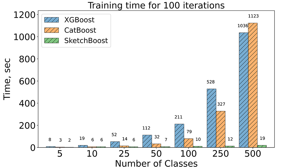
Figure 4: Training time of XGBoost, CatBoost, and SkechBoost in the same experiment as in Figure 1. Here SketchBoost uses Random Projection with sketch dimension $k=5$. Further details are given in Section B.7.

In this paper, we presented effective methods to speed up GBDT on multioutput tasks. These methods are generic and can be easily integrated into any single-tree GBDT realization. On real-world datasets, these methods achieve comparable and sometimes even better results to the existing state-of-the-art GBDT implementations but in remarkably less time. The proposed methods are implemented in SketchBoost which itself is a part of our Python-based implementation of GBDT called Py-Boost. Figure 4 concludes this paper by showing the gain in training time of SkechBoost in the same experiment as in Figure 1 from the Introduction.

Appendix A Additional Information on Sketched Split Scoring Methods.

This section provides additional information on sketched split scoring methods from Section 3. Let us recall that the scoring function $S(R)$ for a leaf $R$ is given by

$$S_{G}(R)=\frac{\bigl{\|}G^{\top}v_{R}\bigr{\|}^{2}}{|R|+\lambda},\quad\text{where}\ \,G=\begin{pmatrix}g_{1}^{1}&g_{1}^{2}&\ldots&g_{1}^{d}\\ \vdots&\vdots&\ddots&\vdots\\ g_{n}^{1}&g_{n}^{2}&\ldots&g_{n}^{d}\\ \end{pmatrix}\ \,\text{and}\ \,v_{R}=\begin{pmatrix}[x_{1}\in R]\\ \vdots\\ [x_{n}\in R]\\ \end{pmatrix}.$$

Here $G\in\mathbb{R}^{n\times d}$ is the matrix whose $i$-th row consists of gradient values $(g_{i}^{1},\ldots,g_{i}^{d})=\nabla_{a}l(y_{i},a)|_{a=F_{t-1}(x_{i})}$, $i=1,\ldots,n$, and $v_{R}$ is the indicator vector of leaf $R$ (its $i$-th component equals $1$ if $x_{i}\in R$ and $0$ otherwise). To reduce the complexity of computing $S_{G}(R)$ in $d$, we approximate $S_{G}(R)$ with $S_{G_{k}}(R)$ for some sketch matrix $G_{k}\in\mathbb{R}^{n\times k}$ with $k\ll d$. The error of this approximation is measured by

$$\operatorname{Error}(S_{G},S_{G_{k}})=\sup_{R}\bigl{|}S_{G}(R)-S_{G_{k}}(R)\bigr{|}.$$ (8)

The supremum here is taken over all possible leaves $R$, so that we aim at the optimization of the worst case. The reason for this is that we want the proposed approximation to be universal and uniformly accurate for all splits we will possibly iterate over.

Given the two matrices $G$ and $G_{k}$, the optimization problem from (8) is an instance of Integer Programming problem and hence is NP-complete. To obtain a closed-form solution, one needs to iterate through all possible leaves $R$ (that is, through all possible vectors $v_{R}$ with $0/1$ entries). Since the brute force is not an option in our case, we will replace this problem with a relaxed one and will look for nearly-optimal solutions. We will show that reasonably good upper bounds on the error are obtained when $GG^{\top}$ is well approximated with $G_{k}G_{k}^{\top}$ in the operator norm; see Lemma A.1. This observation links our problem to Approximate Matrix Multiplication (AMM). In the next sections, we review some deterministic and random methods from AMM and apply them to construct nearly optimal sketches $G_{k}$.

Auxiliary Lemma.

First let us state an auxiliary lemma which bounds the approximation error from (8) with the distance between $GG^{\top}$ and $G_{k}G_{k}^{\top}$ is the operator norm.

Lemma A.1.

Let $G\in\mathbb{R}^{n\times d}$ and $G_{k}\in\mathbb{R}^{n\times k}$ be any two matrices. Then

$$\operatorname{Error}(S_{G},S_{G_{k}})\leq\bigl{\|}GG^{\top}-G_{k}G_{k}^{\top}\bigr{\|}.$$ (9)

Proof.

A direct computation yields

$$\sup_{R}\bigl{|}S_{G}(R)-S_{G_{k}}(R)\bigr{|} =\sup_{R}\left|\frac{\|G^{\top}v_{R}\|^{2}-\|G_{k}^{\top}v_{R}\|^{2}}{|R|+\lambda}\right|$$

$$\leq\sup_{R}\frac{\|GG^{\top}-G_{k}G_{k}^{\top}\|\|v_{R}\|^{2}}{|R|+\lambda}.$$

Since $\lambda>0$ and $\|v_{R}\|^{2}\leq|R|$ ($v_{R}$ has $|R|$ non-zero entries equal to $1$), the assertion follows. ∎

Note that in practice we do not need to compute $GG^{\top}$. Lemma A.1 only provides a theoretical bound which will be used further. This bound is universal for all possible leafs $R$ and involves only the gradient matrix $G$ and its sketch $G_{k}$.

A.1 Truncated SVD

We start with the Truncated SVD algorithm since, by the matrix approximation lemma (the Eckart-Young-Mirsky theorem), it provides the optimal deterministic solution to AMM. The following proposition summarizes its performance.

Proposition A.2.

Let $G\in\mathbb{R}^{n\times d}$ be any matrix. Let also $G_{k}\in\mathbb{R}^{n\times k}$ be the best $k$-rank approximation of $G$ provided by the Truncated SVD. Then

$$\operatorname{Error}(S_{G},S_{G_{k}})\leq\sigma^{2}_{k+1}(G),$$

where $\sigma^{2}_{k+1}(G)$ is $(k+1)$ largest singular value of $G$.

Proof.

Let $G=U\Sigma V^{\top}$ be the full SVD of $G$. Let also $G_{k}=U_{k}\Sigma_{k}$ be the $k$-rank Truncated SVD of $G$ where we keep only largest $k$ singular values and corresponding columns in $U$. Using Lemma A.1, we get

$$\sup_{R}\bigl{|}S_{G}(R)-S_{G_{k}}(R)\bigr{|}\leq\bigl{\|}GG^{\top}-G_{k}G_{k}^{\top}\bigr{\|}=\bigl{\|}U\Sigma^{2}U^{\top}-U_{k}\Sigma_{k}^{2}U_{k}^{\top}\bigr{\|}.$$

Now the Eckart–Young–Mirsky theorem (for the spectral norm) yelds

$$\bigl{\|}U\Sigma^{2}U^{\top}-U_{k}\Sigma_{k}^{2}U_{k}^{\top}\bigr{\|}=\sigma^{2}_{s+1}(G),$$

which finishes the proof. ∎

This proposition asserts that to speed up the split search, the gradient matrix $G$ with $d$ columns can be replaced by its Truncated SVD estimate with $k$ columns. As a result, the scoring function $S_{G}$ will not change significantly provided that $(k+1)$ largest singular value of $G$ is small. The parameter $k$ here can be chosen adaptively depending of the spectrum of $G$ and values on $S_{G}$.

We haven’t discussed Truncated SVD in the paper due to its computational complexity which is $O(\min\{nd^{2},n^{2}d\})$; see [Golub and Van Loan, 1996]. As it was discussed in the Introduction, the computational complexity of GBDT scales linearly in the output dimension $d$. Consequently, the application of Truncated SVD will only increase this complexity. Further, we discuss methods with less computational costs.

A.2 Top Outputs

Top Outputs is a straightforward method which constructs the sketch $G_{k}$ by keeping $k$ columns of the gradient matrix $G$ with the largest Euclidian norm.

Proposition A.3.

Let $G\in\mathbb{R}^{n\times d}$ be any matrix. Let also $G_{k}\in\mathbb{R}^{n\times k}$ be the sketch of $G$ given by Top Outputs. Then

$$\operatorname{Error}(S_{G},S_{G_{k}})\leq\sum_{j=k+1}^{d}\|g_{i_{j}}\|^{2}.$$

Proof.

Lemma A.1 implies that

$$\sup_{R}\bigl{|}S_{G}(R)-S_{G_{k}}(R)\bigr{|} \leq\bigl{\|}GG^{\top}-G_{k}G_{k}^{\top}\bigr{\|}.$$

We rewrite $GG^{\top}$ and $G_{k}G_{k}^{\top}$ as an outer product of their columns,

$$GG^{\top}=\sum_{i=1}^{d}g_{i}g_{i}^{\top}\quad\text{and}\quad G_{k}G_{k}^{\top}=\sum_{j=1}^{k}g_{i_{j}}g_{i_{j}}^{\top}.$$

see Section 3.2 for notation. By construction, we have

$$\bigl{\|}GG^{\top}-G_{k}G_{k}^{\top}\bigr{\|}=\Biggr{\|}\sum_{j=k+1}^{d}g_{i_{j}}g_{i_{j}}^{\top}\Biggr{\|}\leq\sum_{j=k+1}^{d}\bigl{\|}g_{i_{j}}\bigr{\|}^{2},$$

and the proof is complete. ∎

This proposition shows that the approximation error is small when we cut out columns of $G$ with a small norm. Top Outputs method is less preferable than Truncated SVD in terms of the approximation error. Nevertheless, here the sketch $G_{k}$ can be computed in time $O(nd)$ which is linear in $d$ contrary to the Truncated SVD.

A.3 Random Sampling

In Random Sampling, we sample columns of $G$ according to probabilities proportional to their Euclidian norm. Before we proceed, let us denote the stable rank of $G$ by

$$\operatorname{sr}(G)=\frac{\|G\|^{2}_{\text{Fr}}}{\|G\|^{2}},$$

where $\|\cdot\|$ denotes the spectral norm. The stable rank is a relaxation of the exact notion of rank. Indeed, one always has $\operatorname{sr}(G)\leq\operatorname{rank}(G)$. But as opposed to the exact rank, it is stable under small perturbations of the matrix. Both exact and stable ranks are usually referred to as the intrinsic dimensionality of a matrix (in data-driven applications matrices tend to have small ranks).

Proposition A.4.

Let $G\in\mathbb{R}^{n\times d}$ be any matrix. Let also $G_{k}\in\mathbb{R}^{n\times k}$ be a sketch obtained by Random Sampling. Then for any $\delta\in(0,1)$, with probability at least $1-\delta$,

$$\operatorname{Error}(S_{G},S_{G_{k}})\leq C_{G,\delta}\,\frac{\|G\|^{2}}{\sqrt{k}},$$

where $C_{G,\delta}$ is a constant depending on $G$ and $\delta$ and is given by

$$C_{G,\delta}=2\sqrt{\operatorname{sr}(G)\log\left(\frac{4\operatorname{sr}(G)}{\delta}\right)}.$$

Proof.

Lemma A.1 yields

$$\sup_{R}\bigl{|}S_{G}(R)-S_{G_{k}}(R)\bigr{|} \leq\bigl{\|}GG^{\top}-G_{k}G_{k}^{\top}\bigr{\|}.$$

Using Theorem 4.2 from [Holodnak and Ipsen, 2015], we obtain that for any $\varepsilon,\delta\in(0,1)$ with probability at least $1-\delta$,

$$\|GG^{\top}-G_{k}G_{k}^{\top}\|\leq\varepsilon\|G\|^{2}$$

provided that $k\geq 3\operatorname{sr}(G)\ln(\frac{4r}{\delta})/\varepsilon^{2}$. Solving the latter inequality with respect to $\varepsilon$, we establish the assertion. ∎

This proposition states that the approximation error is, with high probability, of order $\|G\|^{2}/\sqrt{k}$ when the stable rank of $G$ is small. There is no definite answer whether this bound is better than the bounds obtained for other methods. The answer depends on the spectrum of $G$. Moreover, this bound is of probabilistic nature. Nevertheless, Random Sampling has the computational complexity $O(nd)$ and is as fast as Top Outputs.

A.4 Random Projections

Random Projections samples $k$ random linear combinations of columns of G to construct $G_{k}$.

Proposition A.5.

Let $G\in\mathbb{R}^{n\times d}$ be any matrix. Let also $\Pi\in\mathbb{R}^{d\times k}$ be a random matrix filled with independently sampled $\mathcal{N}(0,k^{-1})$ entries. Set $G_{k}=G\Pi$. Then for any $\delta\in(0,1)$, with probability at least $1-\delta$,

$$\operatorname{Error}(S_{G},S_{G_{k}})\leq C_{G,\delta}\,\frac{\|G\|^{2}}{\sqrt{k}},$$

where $C_{G,\delta}$ is a constant depending on $G$ and $\delta$ and is given by

$$C_{G,\delta}=c\sqrt{\operatorname{sr}(G)+\ln\left(\frac{1}{\delta}\right)}.$$

for some absolute constant $c>0$.

Proof.

Using Lemma A.1, we get

$$\sup_{R}\bigl{|}S_{G}(R)-S_{G_{k}}(R)\bigr{|} \leq\bigl{\|}GG^{\top}-G_{k}G_{k}^{\top}\bigr{\|}.$$

Now Theorem 1 from [Kyrillidis et al., 2014] implies that for any $\varepsilon,\delta\in(0,1)$ with probability at least $1-\delta$,

$$\|GG^{\top}-G_{k}G_{k}^{\top}\|\leq\varepsilon\|G\|^{2}$$

provided that $k\geq c\left(\operatorname{sr}(G)+\ln\ln(\frac{1}{\varepsilon})+\ln(\frac{1}{\delta})\right)/\varepsilon^{2}$. If we set

$$\varepsilon=c^{\prime}\sqrt{(\operatorname{sr}(G)+\ln(\tfrac{1}{\delta}))\big{/}k}$$

for another absolute constant $c^{\prime}$, the assertion follows. ∎

Comparing to Proposition A.4, this bound is slightly better in terms of $C_{G,\delta}$. But the sketch $G_{k}$ here can be computed only in time $O(ndk)$ since it requires multiplication of $G$ and $\Pi$. To speed up it, one can use Fast JL transform [Ailon and Chazelle, 2009] or Sparse JL transform [Dasgupta, Kumar, and Sarlos, 2010], [Kane and Nelson, 2014].

Appendix B Experiment Details

We remind the reader that our Python-based GPU implementation of GBDT called Py-Boost is available on GitHub. The code to reproduce the experiments is also available on GitHub.

B.1 About Py-Boost

As was mentioned in the original paper, Py-Boost is written in Python and follows the classic scheme described in [Chen and Guestrin, 2016]. Meanwhile, it is a simplified version of gradient boosting, and hence it has a few limitations. Some of these limitations have been made to speed up computations, some — to remove unnecessary for our purposes features presented in modern gradient boosting toolkits (for example, categorical data handling). The complete list of these limitations is the following. Py-Boost supports: (a) computations only on GPU, (b) only the depth-wise tree growth policy, (c) only numeric features (with possibly NaN values), and (d) only histogram algorithm for split search (maximum number of bins for each feature is limited to $256$).

Py-Boost uses GPU Python libraries such as CuPy, Numba, and CuML to speed up computations. XGBoost and CatBoost frameworks are also evaluated in the GPU mode where possible (CatBoost is evaluated on CPU on multilabel classification and multioutput regression tasks since it does not support them on GPU).

B.2 Experiment design

In our numerical experiments, we compare SketchBoost Full, SketchBoost with sketching strategies (Top Outputs, Random Sampling, Random Projections), XGBoost (v1.6.0) which uses the one-vs-all strategy, and CatBoost (v1.0.5) which uses the single-tree strategy, and a popular deep learning model for tabular data TabNet (v3.1.1). In this section, we discuss experiment design for GBDTs; details for TabNet are given in Section B.4 below. The experiments are conducted on $9$ real-world publicly available datasets from Kaggle, OpenML, and Mulan website for multiclass/multilabel classification and multitask regression. Datasets details are given in Table 5.

Table 5: Dataset statistics.

Dataset	Task	Rows	Features	Classes/Labels/Targets	Source	Download
Otto	multiclass	61 878	93	9	Kaggle	Link
SF-Crime	multiclass	878 049	10	39	Kaggle	Link
Helena	multiclass	65 196	27	100	OpenML	Link
Dionis	multiclass	416 188	60	355	OpenML	Link
Mediamill	multilabel	43 907	120	101	Mulan	Link
MoA	multilabel	23 814	876	206	Kaggle	Link
Delicious	multilabel	16 105	500	983	Mulan	Link
RF1	multitask	9125	64	8	Mulan	Link
SCM20D	multitask	8966	61	16	Mulan	Link

We remind the reader that if there is no official train/test split, we split the data into train and test sets with ratio 80%-20%. Datasets taken from Kaggle have the official train/test split, but since the platform hides the test set, we split the train test into the new train and test sets. Some of the datasets required data preprocessing since they contained categorical and datetime features (they cannot be handled by all of the GBDT implementations on the fly). The code for data preprocessing step is also available on GitHub.

Experiments are performed on the server under OS Ubuntu 18.04 with 4 NVidia Tesla V100 32 GB GPUs, 48 cores CPU Intel(R) Xeon(R) Platinum 8168 CPU @ 2.70GHz and 386 GB RAM. We run all the tasks on 8 CPU threads and single GPU if needed.

The experiments are divided into two the following parts:

• Parameter tuning. Here we optimize hyperparameters for XGBoost and CatBoost. For SketchBoost we use the same hyperparameters as for CatBoost (to speed up the parameter tuning process; we do not expect that hyperparameters will vary much since we use the same tree building strategy). At this stage, parameters are estimated by 5-fold cross-validation using only the train set.

• Model evaluation. After the best parameters are found, we refit all the models using a longer training time. The models are trained again by 5-fold cross-validation, but their quality is estimated on the test set. The final score and time metrics are computed as the average of 5 values given by 5 models from the cross-validation loop.

During the parameter tuning, we use a slightly different setup (higher learning rate and less maximum number of rounds) to evaluate more trials and find a better hyperparameter set. Table 6 provides the associate details.

Table 6: Setup for the parameter tuning and model evaluation stages.

Stage	Learning Rate	Max Number of Rounds	Early Stopping Rounds	Quality Estimation
Parameter tuning	0.05	5000	200	cross-validation
Models evaluation	0.015	20000	500	test set

Since all the models are trained using cross-validation, the optimal number of boosting rounds is determined adaptively by early stopping on the validation fold. In this setup, the test set is used only for quality evaluation. As the primary quality measure, we use the cross-entropy for classification and RMSE for regression. But for the sake of completeness, we also report the accuracy for classification and R-squared for regression, see Section B.5.

B.3 Hyperparameter tuning

It is quite challenging to perform a fair test among all the frameworks. Evaluation results depend not only on the sketching method or the strategy used to handle a multioutput problem (one-vs-all or single-tree), but also on hyperparameter setting and implementation details. To make our comparison as fair as possible, we perform a hyperparameter optimization for XGBoost and CatBoost using the Optuna framework that performs a sequential model-based optimization by the Tree-structured Parzen Estimator (TPE) method; see [Bergstra, Bardenet, Bengio, and Kégl, 2011]. The list of optimized hyperparameters is given in Table 7.

Table 7: Optimized hyperparameters.

Parameter	Framework	Type	Default value	Search space	Log
Maximal Tree Depth	All	Int	6	[3:12]	False
Min Child Weight	XGBoost	Float	1e-5	[1e-5:10]	True
Min Data In Leaf	CatBoost	Int	1	[1: 100]	True
L2 leaf regularization	All	Float	1	[0.1: 50]	True
Rows Sampling Rate	All	Float	1.0	[0.5: 1]	False

Note: Minimal data in leaf and Minimal child weight both control the leaf size but in different frameworks. It is the reason why they have different scales in the table.

The optimal number of rounds is determined by early stopping for the fixed learning rate; see Section B.2 for the details. There are some other parameters of GBDT that are not optimized since not all the frameworks allow to change them. For example, the columns sampling rate cannot be changed in CatBoost in the GPU mode, and only the depth-wise grow policy is supported in SketchBoost.

The tuning process is organized in the following way:

• Safe run. First, we perform a single run with a set of parameters that are listed in Table 7 as default. These hyperparameters are close to the framework’s default settings and can be considered as a safe option in the case when a good set of parameters is not found in the time limit.

• TPE search. Then we perform 30 iterations of parameters search with the Optuna framework. As it was mentioned, the training time may be quite long for the multioutput tasks, so we limit the search time to 24 hours in order to finish it in a reasonable amount of time.

• Selection. Finally, we determine the best parameters as the ones that achieve the best performance between all trials (both safe and TPE).

The best hyperparameters and the number of successful (finished in time) trials are given in Table 8.

Table 8: Results for hyperparameter optimization.

Dataset	Framework	Min	Min	Rows sampling	Max	L2 leaf	Completed
		data in leaf	child weight	rate	depth	regularization	trials
Otto	CatBoost	47	–	0.89	10	3.83	31
	XGBoost	–	0.00001	0.58	12	23.57	31
SF-Crime	CatBoost	2	–	0.94	11	2.65	31
	XGBoost	–	1.25682	0.92	12	8.37	24
Helena	CatBoost	2	–	0.55	6	12.77	31
	XGBoost	–	0.33734	0.50	6	23.33	31
Dionis	CatBoost	1	–	1.0	6	1.0	6
	XGBoost	–	0.00001	1.0	6	1.0	3
Mediamill	CatBoost	10	–	0.76	8	11.16	8
	XGBoost	–	1.90469	0.68	12	39.30	31
MoA	CatBoost	30	–	0.88	4	1.03	10
	XGBoost	–	0.00342	0.93	3	0.37	31
Delicious	CatBoost	76	–	0.62	12	13.05	5
	XGBoost	–	0.06235	0.72	11	33.22	10
RF1	CatBoost	1	–	0.85	10	9.96	31
	XGBoost	–	0.00431	0.68	5	12.22	31
SCM20D	CatBoost	5	–	0.99	12	6.57	31
	XGBoost	–	9.93770	0.80	6	1.44	31

B.4 Details on TabNet

Here we provide additional details on TabNet [Arik and Pfister, 2021]. We consider PyTorch (v1.7.0)-based implementation pytorch-tabnet library (v3.1.1). The evaluation is performed on the same datasets, under the same experiment setup including train/validation/test splits, and using the same hardware as described in Section B.2. TabNet hyperparameters are taken from the original paper [Arik and Pfister, 2021] except the learning rate, batch size, and the number of epochs for train and early stopping. These hyperparameters are tuned in the following way:

• The optimal learning rate is tuned using the Optuna framework from the range ($1e-5$; $1e-1$) in the log scale in the same way at it is described in Section B.3 (one single safe run with learning rate $2e-2$ and then TPE search for $10$ trials with time limit of $24$ hours). The best trial is selected based on the cross-validation score and then it is evaluated on the test set.

• The optimal number of epochs is selected via early stopping with $16$ epochs with no improve. Maximal number of epochs is limited to $500$.

• The batch size is selected depending on the dataset size: $256$ for data with less than $50$k rows, $512$ for $50$-$100$k rows, and $1024$ for more then $100$k rows.

The proposed values are quite typical for tabular data according to [Gorishniy, Rubachev, Khrulkov, and Babenko, 2021], [Fiedler, 2021], and [Arik and Pfister, 2021]. The unsupervised pretrain proposed in the paper is also used on each cross-validation iteration. The selected hyperparameters are listed in the Table 9 below.

Table 9: Results for hyperparameter optimization for TabNet.

Dataset	Learning	Batch	Completed
	rate	size	trials
Otto	0.0394	512	11
SF-Crime	0.0200	1024	3
Helena	0.0080	512	9
Dionis	0.0110	1024	7
Mediamill	0.0315	256	11
MoA	0.0200	256	10
Delicious	0.0231	256	11
RF1	0.0200	256	11
SCM20D	0.0200	256	11

B.5 Additional experimental results

Figure 5: Dependence of test errors (cross-entropy for classification and RMSE for regression) on sketch dimension $k$ for all datasets.

Table 10: Test errors (cross-entropy for classification and RMSE for regression) $\pm$ their standard deviation.

		Dataset
Algorithm		Otto	SF-Crime	Helena	Dionis	Mediamill	MoA	Delicious	RF1	SCM20D
XGBoost		0.4599	2.2208	2.5889	0.3502	0.0758	0.0166	0.0620	0.9250	89.1045
		$\pm$0.0027	$\pm$0.0008	$\pm$0.0031	$\pm$0.0019	$\pm$1.1e-04	$\pm$2.1e-05	$\pm$3.3e-05	$\pm$0.0307	$\pm$0.4950
CatBoost		0.4658	2.2036	2.5698	0.3085	0.0754	0.0161	0.0614	0.8975	90.9814
		$\pm$0.0032	$\pm$0.0005	$\pm$0.0025	$\pm$0.0010	$\pm$1.1e-04	$\pm$2.6e-05	$\pm$5.2e-05	$\pm$0.0383	$\pm$0.3652
TabNet		0.5363	2.4819	2.7197	0.4753	0.0859	0.0193	0.0664	3.7948	87.3655
		$\pm$0.0063	$\pm$0.0199	$\pm$0.0235	$\pm$0.0126	$\pm$3.3e-03	$\pm$3.0e-04	$\pm$8.0e-04	$\pm$1.5935	$\pm$1.3316
SketchBoost Full		0.4697	2.2067	2.5865	0.3114	0.0747	0.0160	0.0619	1.1687	91.0142
		$\pm$0.0029	$\pm$0.0003	$\pm$0.0025	$\pm$0.0008	$\pm$1.3e-04	$\pm$9.0e-06	$\pm$5.5e-05	$\pm$0.0835	$\pm$0.3396
Top Outputs	$k=1$	0.4975	2.2282	2.5923	0.3339	0.0745	0.0169	0.0624	1.3151	90.7613
		$\pm$0.0030	$\pm$0.0004	$\pm$0.0024	$\pm$0.0017	$\pm$1.3e-04	$\pm$4.1e-05	$\pm$6.3e-05	$\pm$0.0721	$\pm$0.3988
	$k=2$	0.4964	2.2284	2.5938	0.3217	0.0745	0.0168	0.0624	1.2823	89.5284
		$\pm$0.0041	$\pm$0.0001	$\pm$0.0025	$\pm$0.0019	$\pm$1.4e-04	$\pm$2.0e-05	$\pm$5.1e-05	$\pm$0.1363	$\pm$0.8352
	$k=5$	0.4715	2.2183	2.5974	0.3155	0.0745	0.0168	0.0623	1.1860	88.7442
		$\pm$0.0035	$\pm$0.0005	$\pm$0.0018	$\pm$0.0013	$\pm$1.1e-04	$\pm$1.6e-05	$\pm$6.3e-05	$\pm$0.1365	$\pm$0.6345
	$k=10$	–	2.2116	2.5987	0.3151	0.0746	0.01660	0.0622	–	89.8727
		–	$\pm$0.0025	$\pm$0.0019	$\pm$0.0014	$\pm$1.0e-04	$\pm$2.5e-05	$\pm$5.5e-05	–	$\pm$0.3126
	$k=20$	–	2.2070	2.5945	0.3146	0.0747	0.0163	0.0622	–	–
		–	$\pm$0.0005	$\pm$0.0020	$\pm$0.0010	$\pm$1.1e-04	$\pm$2.2e-05	$\pm$6.2e-05	–	–
Random Sampling	$k=1$	0.4677	2.2140	2.5693	0.3175	0.0745	0.0163	0.0622	1.1495	87.9358
		$\pm$0.0019	$\pm$0.0003	$\pm$0.0022	$\pm$0.0009	$\pm$1.3e-04	$\pm$2.0e-05	$\pm$6.4e-05	$\pm$0.0674	$\pm$0.4111
	$k=2$	0.4636	2.2083	2.5710	0.3089	0.0745	0.0162	0.0621	0.9965	86.7842
		$\pm$0.0025	$\pm$0.0003	$\pm$0.0032	$\pm$0.0012	$\pm$9.1e-05	$\pm$1.5e-05	$\pm$5.5e-05	$\pm$0.1011	$\pm$0.5546
	$k=5$	0.4642	2.2052	2.5730	0.3055	0.0745	0.0161	0.0620	0.9944	86.2964
		$\pm$0.0020	$\pm$0.0005	$\pm$0.0024	$\pm$0.0012	$\pm$9.8e-05	$\pm$1.5e-05	$\pm$5.6e-05	$\pm$0.1014	$\pm$0.4398
	$k=10$	–	2.2041	2.5757	0.3051	0.0745	0.0161	0.0619	–	86.6865
		–	$\pm$0.0005	$\pm$0.0018	$\pm$0.0009	$\pm$1.0e-04	$\pm$1.5e-05	$\pm$5.2e-05	–	$\pm$0.2829
	$k=20$	–	2.2037	2.5759	0.3040	0.0745	0.0160	0.0619	–	–
		–	$\pm$0.0004	$\pm$0.0023	$\pm$0.0013	$\pm$1.1e-04	$\pm$1.0e-05	$\pm$5.9e-05	–	–
Random Projection	$k=1$	0.4566	2.2096	2.5674	0.2848	0.0743	0.0160	0.0621	0.9058	86.1442
		$\pm$0.0023	$\pm$0.0005	$\pm$0.0039	$\pm$0.0012	$\pm$1.1e-04	$\pm$1.0e-05	$\pm$5.9e-05	$\pm$0.0442	$\pm$0.4824
	$k=2$	0.4583	2.2076	2.5673	0.2850	0.0743	0.0160	0.0621	0.9056	85.8061
		$\pm$0.0028	$\pm$0.0006	$\pm$0.0026	$\pm$0.0011	$\pm$1.2e-04	$\pm$2e-05	$\pm$5.9e-05	$\pm$0.0581	$\pm$0.5533
	$k=5$	0.4607	2.2052	2.5681	0.2866	0.0743	0.0160	0.0620	0.9193	85.8565
		$\pm$0.0031	$\pm$0.0006	$\pm$0.0019	$\pm$0.0013	$\pm$1.2e-04	$\pm$1.9e-05	$\pm$5.6e-05	$\pm$0.0781	$\pm$0.3116
	$k=10$	–	2.2043	2.5713	0.2881	0.0743	0.0160	0.0620	-	86.3126
		–	$\pm$0.0003	$\pm$0.0024	$\pm$0.0010	$\pm$1.1e-04	$\pm$1.3e-05	$\pm$5.9e-05	-	$\pm$0.3710
	$k=20$	–	2.2038	2.5730	0.2907	0.0743	0.0160	0.062	–	–
		–	$\pm$0.0004	$\pm$0.0030	$\pm$0.0009	$\pm$1.2e-04	$\pm$6.0e-06	$\pm$6.2e-05	–	–

Table 11: Test errors (accuracy for classification and R-squared for regression) $\pm$ their standard deviation.

		Dataset
Algorithm		Otto	SF-Crime	Helena	Dionis	Mediamill	MoA	Delicious	RF1	SCM20D
XGBoost		0.8238	0.3326	0.3770	0.9193	0.9746	0.9971	0.9826	0.9997	0.9257
		$\pm$0.0010	$\pm$0.0003	$\pm$0.0012	$\pm$0.0007	$\pm$4.3e-05	$\pm$8.0e-06	$\pm$6.0e-06	$\pm$3.2e-05	$\pm$0.0007
CatBoost		0.8213	0.3352	0.3808	0.9234	0.9744	0.9971	0.9825	0.9997	0.9224
		$\pm$0.0012	$\pm$0.0008	$\pm$0.0017	$\pm$0.0003	$\pm$7.6e-05	$\pm$5.0e-06	$\pm$1.7e-05	$\pm$4.1e-05	$\pm$0.0006
TabNet		0.7972	0.2550	0.3503	0.8936	0.9709	0.9967	0.9816	0.9932	0.9281
		$\pm$0.0030	$\pm$0.0037	$\pm$0.0060	$\pm$0.0032	$\pm$1.0e-03	$\pm$5.3e-05	$\pm$9.5e-05	$\pm$0.0037	$\pm$0.0022
SketchBoost Full		0.8223	0.3343	0.3783	0.9227	0.9747	0.9971	0.9824	0.9995	0.9224
		$\pm$0.0021	$\pm$0.0007	$\pm$0.0011	$\pm$0.0004	$\pm$6.8e-05	$\pm$6.0e-06	$\pm$1.4e-05	$\pm$5.5e-05	$\pm$0.0007
Top Outputs	$k=1$	0.8172	0.3275	0.3773	0.9192	0.9747	0.9970	0.9823	0.9992	0.9228
		$\pm$0.0022	$\pm$0.0006	$\pm$0.0014	$\pm$0.0006	$\pm$4.9e-05	$\pm$7.0e-06	$\pm$2.0e-05	$\pm$6.1e-05	$\pm$0.0006
	$k=2$	0.8171	0.3275	0.3772	0.9214	0.9747	0.9970	0.9823	0.9993	0.9249
		$\pm$0.0016	$\pm$0.0008	$\pm$0.0021	$\pm$0.0004	$\pm$4.7e-05	$\pm$4.0e-06	$\pm$2.0e-05	$\pm$1.2e-04	$\pm$0.0013
	$k=5$	0.8210	0.3315	0.3760	0.9229	0.9747	0.9970	0.9823	0.9994	0.9262
		$\pm$0.0016	$\pm$0.0003	$\pm$0.0019	$\pm$0.0004	$\pm$5.8e-05	$\pm$1.2e-05	$\pm$1.9e-05	$\pm$9.2e-05	$\pm$0.0010
	$k=10$	–	0.3333	0.3757	0.9229	0.9747	0.997	0.9824	–	0.9243
		–	$\pm$0.0003	$\pm$0.0013	$\pm$0.0003	$\pm$2.8e-05	$\pm$5.0e-06	$\pm$1.5e-05	–	$\pm$0.0005
	$k=20$	–	0.3349	0.3766	0.9227	0.9747	0.9971	0.9824	–	–
		–	$\pm$0.0006	$\pm$0.0008	$\pm$0.0007	$\pm$6.5e-05	$\pm$9.0e-06	$\pm$1.6e-05	–	–
Random Sampling	$k=1$	0.8228	0.3320	0.3821	0.9224	0.9746	0.9971	0.9824	0.9995	0.9276
		$\pm$0.0011	$\pm$0.0002	$\pm$0.0009	$\pm$0.0005	$\pm$5.6e-05	$\pm$5e-06	$\pm$2.0e-05	$\pm$5.4e-05	$\pm$0.0007
	$k=2$	0.8236	0.3338	0.3827	0.9243	0.9746	0.9971	0.9824	0.9996	0.9293
		$\pm$0.0025	$\pm$0.0003	$\pm$0.0015	$\pm$0.0003	$\pm$4.8e-05	$\pm$5.0e-06	$\pm$8.0e-06	$\pm$6.3e-05	$\pm$0.0009
	$k=5$	0.8231	0.3348	0.3795	0.9250	0.9746	0.9971	0.9824	0.9996	0.9301
		$\pm$0.0018	$\pm$0.0002	$\pm$0.0022	$\pm$0.0002	$\pm$4.0e-05	$\pm$1.2e-05	$\pm$1.3e-05	$\pm$6.0e-05	$\pm$0.0007
	$k=10$	–	0.3351	0.3793	0.9250	0.9746	0.9972	0.9824	–	0.9295
		–	$\pm$0.0004	$\pm$0.0018	$\pm$0.0002	$\pm$4.1e-05	$\pm$1.2e-05	$\pm$8.0e-06	–	$\pm$0.0004
	$k=20$	–	0.3353	0.3795	0.9251	0.9746	0.9972	0.9824	–	–
		–	$\pm$0.0005	$\pm$0.0017	$\pm$0.0005	$\pm$5.6e-05	$\pm$9.0e-06	$\pm$1.7e-05	–	–
Random Projection	$k=1$	0.8258	0.3338	0.3834	0.9285	0.9747	0.9971	0.9824	0.9997	0.9304
		$\pm$0.0010	$\pm$0.0003	$\pm$0.0033	$\pm$0.0004	$\pm$1.7e-05	$\pm$6.0e-06	$\pm$1.6e-05	$\pm$3.7e-05	$\pm$0.0008
	$k=2$	0.8255	0.3344	0.3836	0.9287	0.9748	0.9971	0.9824	0.9997	0.9309
		$\pm$0.0023	$\pm$0.0005	$\pm$0.0019	$\pm$0.0002	$\pm$5.6e-05	$\pm$3.0e-06	$\pm$1.8e-05	$\pm$4.4e-05	$\pm$0.0008
	$k=5$	0.8251	0.3351	0.3835	0.9281	0.9748	0.9971	0.9824	0.9997	0.9308
		$\pm$0.0023	$\pm$0.0005	$\pm$0.0018	$\pm$0.0002	$\pm$4.0e-05	$\pm$1.1e-05	$\pm$7.0e-06	$\pm$5.4e-05	$\pm$0.0005
	$k=10$	–	0.3355	0.3824	0.9279	0.9748	0.9971	0.9824	-	0.9301
		–	$\pm$0.0003	$\pm$0.0022	$\pm$0.0002	$\pm$4.0e-05	$\pm$6.0e-06	$\pm$9.0e-06	-	$\pm$0.0006
	$k=20$	–	0.3357	0.3805	0.9275	0.9747	0.9971	0.9824	–	–
		–	$\pm$0.0004	$\pm$0.0025	$\pm$0.0002	$\pm$2.9e-05	$\pm$5.0e-06	$\pm$1.2e-05	–	–

Figure 6: Training time per fold in seconds for the best sketching dimension $k$.

Table 12: Training time per fold in seconds for all sketching dimensions $k$.

		Dataset
Algorithm		Otto	SF-Crime	Helena	Dionis	Mediamill	MoA	Delicious	RF1	SCM20D
XGBoost		1244	4016	1036	18635	2074	376	15795	315	1432
CatBoost		73	659	436	18600	10164	9398	20120	804	798
TabNet		903	2563	1196	1853	1231	672	2902	207	296
SketchBoost Full		131	1146	355	23919	1777	696	19553	413	597
Top Outputs	$k=1$	129	174	154	783	251	40	213	351	458
	$k=2$	126	207	151	810	276	45	229	364	476
	$k=5$	113	270	146	1003	313	59	274	369	499
	$k=10$	–	425	138	1293	386	69	375	–	551
	$k=20$	–	705	156	1889	529	103	575	–	–
Random Sampling	$k=1$	104	198	180	835	263	61	230	347	485
	$k=2$	102	219	180	880	273	75	243	354	491
	$k=5$	116	299	185	1087	319	104	314	396	528
	$k=10$	–	422	198	1404	399	135	432	–	590
	$k=20$	–	676	213	2038	559	189	664	–	–
Random Projection	$k=1$	89	136	109	419	235	26	212	331	466
	$k=2$	87	159	113	464	243	29	235	340	479
	$k=5$	107	233	116	629	294	39	295	393	528
	$k=10$	–	365	128	895	369	55	436	–	594
	$k=20$	–	612	149	1417	527	87	1259	–	–

Table 13: Number of boosting iterations to convergence (for GBDTs). (Although the number of iterations for XGBoost is small, it uses the one-vs-all strategy, and therefore the actual amount of trees in the ensemble equals this number multiplied by the output size $d$.)

	SketchBoost				Baseline
Dataset	Top Outputs	Random Sampling	Random Projection	SketchBoost Full	CatBoost	XGBoost
	(for the best $k$)	(for the best $k$)	(for the best $k$)	(multioutput)	(multioutput)	(one-vs-all)
Multiclass classification
Otto (9 classes)	4799	5424	5201	4424	5534	2142
SF-Crime (39 classes)	3790	3726	3611	3754	3993	1212
Helena (100 classes)	15042	16975	11670	13492	11238	1563
Dionis (355 classes)	17039	17990	11509	18519	19858	2681
Multilabel classification
Mediamill (101 labels)	18623	19961	17826	17927	8983	1878
MoA (206 labels)	2606	5542	2093	2240	4239	471
Delicious (983 labels)	7063	8015	7541	6911	3956	1611
Multitask regression
RF1 (8 tasks)	16102	17076	16815	17001	19999	19994
SCM20D (16 tasks)	19992	19991	19993	19992	19998	19998

B.6 Comparison with GBDT-MO

Here we provide details on comparison of SketchBoost and CatBoost with GBDT-MO and GBDT-MO (sparse) introduced in [Zhang and Jung, 2021]. The GBDT-MO implementation is evaluated on CPU utilizing 8 threads per run (as it was done before). The experiment design and datasets are taken from original paper [Zhang and Jung, 2021]. For all the evaluated algorithms, we use hyperparameters provided in the original paper. For GBDT-MO, we use the best sparsity parameter $K$ which is also provided in the original paper. The only difference in our experiments is model training and evaluation which is done using 5-fold cross-validation (see Section B.2) instead of using the test set for both early stopping and performance evaluation (as was done in the experiments for GBDT-MO). We argue the latter method leads to the effect of quality overestimation. We also note that in the original paper results for GBDT-MO (sparse) are provided only for 4 datasets out of 6 datasets considered (and we also use only these 4 datasets). As it is done in the original paper, we use accuracy as the performance measure. The experimental results are given below.

Table 14: Comparison with GBDT-MO. Test scores (accuracy for classification and RMSE for regression) and their standard deviation for all sketching dimensions $k$.

		Dataset
Algorithm		MNIST	Caltech	NUS-WIDE	MNIST-REG
		(10 classes)	(101 classes)	(81 labels)	(24 tasks)
CatBoost		0.9684$\pm$0.004	0.5049$\pm$0.0167	0.9893$\pm$0.0001	0.2708$\pm$0.0023
GBDT-MO Full		0.976$\pm$0.004	0.4469$\pm$0.059	0.9891$\pm$0.0002	0.2723$\pm$0.0026
GBDT-MO (sparse)		0.9758$\pm$0.0048	0.4796$\pm$0.0375	0.9892$\pm$0.0006	0.2736$\pm$0.0017
SketchBoost Full		0.973$\pm$0.0028	0.5549$\pm$0.008	0.9893$\pm$0.0002	0.266$\pm$0.0019
Random Sampling	$k=1$	0.973$\pm$0.0045	0.5704$\pm$0.0273	0.9892$\pm$0.0003	0.2671$\pm$0.0011
	$k=2$	0.975$\pm$0.0034	0.5704$\pm$0.0174	0.9891$\pm$0.0003	0.2678$\pm$0.0015
	$k=5$	0.9755$\pm$0.0042	0.5599$\pm$0.0146	0.9887$\pm$0.0002	0.2671$\pm$0.0012
	$k=10$	0.9753$\pm$0.0007	0.5623$\pm$0.0165	0.989$\pm$0.0002	0.2661$\pm$0.0019
	$k=20$	–	0.5691$\pm$0.0127	0.9889$\pm$0.0001	0.2665$\pm$0.0014
Random Projection	$k=1$	0.9737$\pm$0.0023	0.5623$\pm$0.0159	0.9897$\pm$0.0003	0.2657$\pm$0.0018
	$k=2$	0.9722$\pm$0.0037	0.5537$\pm$0.0064	0.9893$\pm$0.0004	0.2661$\pm$0.002
	$k=5$	0.974$\pm$0.0032	0.5605$\pm$0.0137	0.9896$\pm$0.0003	0.2658$\pm$0.0013
	$k=10$	0.9722$\pm$0.0045	0.5358$\pm$0.0157	0.9893$\pm$0.0004	0.2663$\pm$0.0007
	$k=20$	–	0.5488$\pm$0.0332	0.9892$\pm$0.0004	0.2654$\pm$0.0012

Table 15: Comparison with GBDT-MO. Training time per fold in seconds for all sketching dimensions $k$.

		Dataset
Algorithm		MNIST	Caltech	NUS-WIDE	MNIST-REG
		(10 classes)	(101 classes)	(81 labels)	(24 tasks)
CatBoost		156	136	13857	964
GBDT-MO Full		362	776	2606	210
GBDT-MO (sparse)		399	1312	3660	163
SketchBoost Full		46	13	87	90
Random Sampling	$k=1$	66	15	36	110
	$k=2$	99	42	145	85
	$k=5$	102	40	148	98
	$k=10$	88	41	151	120
	$k=20$	–	40	158	78
Random Projection	$k=1$	45	16	72	38
	$k=2$	70	13	71	38
	$k=5$	66	15	73	51
	$k=10$	70	14	49	44
	$k=20$	–	14	48	45

B.7 Experiment with synthetic dataset

The aim of this experiment is to illustrate the dependence of the time cost for training $100$ trees on the number of outputs for popular GBDT frameworks on GPU. To do this, we train each framework twice on each task for $100$ and $200$ iterations and then calculate the difference in time. This allows us to estimate the time costs of $100$ boosting iterations regardless the constant time costs such as features quantization and data transfer.

In more detail, since our goal is not to measure model quality and since we need alike datasets that vary only in the output dimension, we consider synthetic datasets generated (with the same feature parameters) by the algorithm proposed in [Guyon, 2003] and implemented in the scikit-learn library (v1.0.2). The dataset features are generated with $2000$k rows and $100$ features ($10$ features ar informative, $20$ features are their linear combinations, and others are redundant). At each iteration, the number of classes is changed over the grid $\{5,10,25,50,100,250,500\}$. After the dataset is generated, we compute and report the time difference between $100$ and $200$ iterations for XGBoost, CatBoost, and SketchBoost with Random Projections (sketch dimension $k=5$). The hardware used in this experiment is the same as described in Section B.2. The main hyperparameters are chosen to be similar for all boosting frameworks. Namely, (1) trees are grown with depth-wise policy with maximal depth limited to $6$, (2) row and column sampling is disabled, (3) learning rate is set to $0.01$, and (4) L2 regularization term is set to $1$, L1 regularization is disabled.

References

- Achlioptas [2003] Dimitris Achlioptas. Database-friendly random projections: Johnson-Lindenstrauss with binary coins. Journal of Computer and System Sciences, 66(4):671–687, 2003.
- Ailon and Chazelle [2009] Nir Ailon and Bernard Chazelle. The Fast Johnson–Lindenstrauss Transform and Approximate Nearest Neighbors. SIAM Journal on Computing, 39:302–322, 2009.
- Akiba et al. [2019] Takuya Akiba, Shotaro Sano, Toshihiko Yanase, Takeru Ohta, and Masanori Koyama. Optuna: A Next-Generation Hyperparameter Optimization Framework. In Proceedings of the 25th ACM SIGKDD international conference on knowledge discovery & data mining, KDD ’19, pages 2623–2631, 2019.
- Alsabti et al. [1998] Khaled Alsabti, Sanjay Ranka, and Vineet Singh. CLOUDS: A Decision Tree Classifier for Large Datasets. In Proceedings of the Fourth International Conference on Knowledge Discovery and Data Mining, KDD’98, pages 2–8. AAAI Press, 1998.
- Appel et al. [2013] Ron Appel, Thomas Fuchs, Piotr Dollár, and Pietro Perona. Quickly Boosting Decision Trees: Pruning Underachieving Features Early. In Proceedings of the 30th International Conference on International Conference on Machine Learning, number 3 in ICML’13, pages 594–602. PMLR, 2013.
- Arik and Pfister [2021] Sercan Ö. Arik and Tomas Pfister. Tabnet: Attentive Interpretable Tabular Learning. Proceedings of the AAAI Conference on Artificial Intelligence, 35(8):6679–6687, 2021.
- Bergstra et al. [2011] James Bergstra, Rémi Bardenet, Yoshua Bengio, and Balázs Kégl. Algorithms for Hyper-Parameter Optimization. In Proceedings of the 24th International Conference on Neural Information Processing Systems, NIPS’11, pages 2546–2554. Curran Associates Inc., 2011.
- Borisov et al. [2021] Vadim Borisov, Tobias Leemann, Kathrin Seßler, Johannes Haug, Martin Pawelczyk, and Gjergji Kasneci. Deep Neural Networks and Tabular Data: A Survey, 2021.
- Breiman [1996] Leo Breiman. Bagging Predictors. Machine learning, 24(2):123–140, 1996.
- Chen and Guestrin [2016] Tianqi Chen and Carlos Guestrin. XGBoost: A Scalable Tree Boosting System. In Proceedings of the 22nd ACM SIGKDD International Conference on Knowledge Discovery and Data Mining, KDD ’16, pages 785–794. Association for Computing Machinery, 2016.
- Cissé et al. [2012] M. Cissé, T. Artières, and Patrick Gallinari. Learning Compact Class Codes for Fast Inference in Large Multi Class Classification. In Proceedings of the 2012th European Conference on Machine Learning and Knowledge Discovery in Databases - Volume Part I, ECMLPKDD’12, pages 506–520, 2012.
- Dasgupta et al. [2010] Anirban Dasgupta, Ravi Kumar, and Tamás Sarlos. A Sparse Johnson: Lindenstrauss Transform. In Proceedings of the Forty-Second ACM Symposium on Theory of Computing, STOC ’10, pages 341–350. Association for Computing Machinery, 2010.
- Fiedler [2021] James Fiedler. Simple Modifications to Improve Tabular Neural Networks, 2021.
- Freund [1995] Yoav Freund. Boosting a Weak Learning Algorithm by Majority. Information and Computation, 121(2):256–285, 1995.
- Freund and Schapire [1997] Yoav Freund and Robert E Schapire. A Decision-Theoretic Generalization of On-Line Learning and an Application to Boosting. Journal of Computer and System Sciences, 55(1):119–139, 1997.
- Friedman [2001] Jerome H. Friedman. Greedy function approximation: A gradient boosting machine. The Annals of Statistics, 29(5):1189 – 1232, 2001.
- Friedman [2002] Jerome H. Friedman. Stochastic Gradient Boosting. Computational Statistics & Data Analysis, 38(4):367–378, 2002.
- Golub and Van Loan [1996] Gene H. Golub and Charles F. Van Loan. Matrix Computations. The Johns Hopkins University Press, third edition, 1996.
- Gorishniy et al. [2021] Yury Gorishniy, Ivan Rubachev, Valentin Khrulkov, and Artem Babenko. Revisiting Deep Learning Models for Tabular Data. Advances in Neural Information Processing Systems, 34:18932–18943, 2021.
- Guyon [2003] Isabelle Guyon. Design of experiments of the NIPS 2003 variable selection benchmark. In NIPS 2003 workshop on feature extraction and feature selection, volume 253, page 40, 2003.
- Holodnak and Ipsen [2015] John T. Holodnak and Ilse C. F. Ipsen. Randomized Approximation of the Gram Matrix: Exact Computation and Probabilistic Bounds. SIAM Journal on Matrix Analysis and Applications, 36:110–137, 2015.
- Hsu et al. [2009] Daniel Hsu, Sham M. Kakade, John Langford, and Tong Zhang. Multi-Label Prediction via Compressed Sensing. In Proceedings of the 22nd International Conference on Neural Information Processing Systems, NIPS’09, pages 772–780. Curran Associates Inc., 2009.
- Ibragimov and Gusev [2019] Bulat Ibragimov and Gleb Gusev. Minimal Variance Sampling in Stochastic Gradient Boosting, 2019.
- Indyk and Motwani [1998] Piotr Indyk and Rajeev Motwani. Approximate Nearest Neighbors: Towards Removing the Curse of Dimensionality. In Proceedings of the Thirtieth Annual ACM Symposium on Theory of Computing, STOC ’98, pages 604–613, 1998.
- Jahrer et al. [2010] Michael Jahrer, Andreas Töscher, and Robert Legenstein. Combining Predictions for Accurate Recommender Systems. In Proceedings of the 16th ACM SIGKDD International Conference on Knowledge Discovery and Data Mining, KDD ’10, pages 693–702, New York, NY, USA, 2010. Association for Computing Machinery.
- Jimenez and Landgrebe [1999] L.O. Jimenez and D.A. Landgrebe. Hyperspectral Data Analysis and Supervised Feature Reduction via Projection Pursuit. IEEE Transactions on Geoscience and Remote Sensing, 37(6):2653–2667, 1999.
- Jin and Agrawal [2003a] Ruoming Jin and Gagan Agrawal. Efficient Decision Tree Construction on Streaming Data. In Proceedings of the Ninth ACM SIGKDD International Conference on Knowledge Discovery and Data Mining, KDD’03, pages 571–576, New York, NY, USA, 2003a. Association for Computing Machinery.
- Jin and Agrawal [2003b] Ruoming Jin and Gagan Agrawal. Communication and Memory Efficient Parallel Decision Tree Construction. In Proceedings of the Third SIAM International Conference on Data Mining, pages 119–129. SIAM, 2003b.
- Johnson and Lindenstrauss [1984] William Johnson and Joram Lindenstrauss. Extensions of lipschitz maps into a hilbert space. Contemporary Mathematics, 26:189–206, 1984.
- Kane and Nelson [2014] Daniel M. Kane and Jelani Nelson. Sparser Johnson-Lindenstrauss Transforms. Journal of the ACM, 61(1), 2014.
- Kapoor et al. [2012] Ashish Kapoor, Raajay Viswanathan, and Prateek Jain. Multilabel Classification using Bayesian Compressed Sensing. In F. Pereira, C.J. Burges, L. Bottou, and K.Q. Weinberger, editors, Advances in Neural Information Processing Systems, volume 25 of NIPS’12, pages 2645–2653. Curran Associates, Inc., 2012.
- Ke et al. [2017] Guolin Ke, Qi Meng, Thomas Finley, Taifeng Wang, Wei Chen, Weidong Ma, Qiwei Ye, and Tie-Yan Liu. LightGBM: A Highly Efficient Gradient Boosting Decision Tree. In Proceedings of the 31st International Conference on Neural Information Processing Systems, NIPS’17, pages 3149–3157. Curran Associates Inc., 2017.
- Kyrillidis et al. [2014] Anastasios Kyrillidis, Michail Vlachos, and Anastasios Zouzias. Approximate Matrix Multiplication with Application to Linear Embeddings. 2014 IEEE International Symposium on Information Theory, pages 2182–2186, 2014.
- Li et al. [2007] Ping Li, Christopher J. C. Burges, and Qiang Wu. McRank: Learning to Rank Using Multiple Classification and Gradient Boosting. In Proceedings of the 20th International Conference on Neural Information Processing Systems, NIPS’07, pages 897–904. Curran Associates Inc., 2007.
- Li et al. [2008] Ping Li, Qiang Wu, and Christopher Burges. McRank: Learning to Rank Using Multiple Classification and Gradient Boosting. In Advances in Neural Information Processing Systems, volume 20. Curran Associates, Inc., 2008.
- Mahoney [2011] Michael W. Mahoney. Randomized Algorithms for Matrices and Data. Foundations and Trends in Machine Learning, 3(2):123–224, 2011.
- Mehta et al. [1996] Manish Mehta, Rakesh Agrawal, and Jorma Rissanen. SLIQ: A Fast Scalable Classifier for Data Mining. In International Conference on Extending Database Technology, pages 18–32. Springer-Verlag, 1996.
- Obermann and Waack [2016] Lennart Obermann and Stephan Waack. Interpretable Multiclass Models for Corporate Credit Rating Capable of Expressing Doubt. Frontiers in Applied Mathematics and Statistics, 2, 2016.
- Prokhorenkova et al. [2018] Liudmila Prokhorenkova, Gleb Gusev, Aleksandr Vorobev, Anna Veronika Dorogush, and Andrey Gulin. CatBoost: Unbiased Boosting with Categorical Features. In Proceedings of the 32nd International Conference on Neural Information Processing Systems, NIPS’18, pages 6639–6649. Curran Associates Inc., 2018.
- Qin et al. [2021] Zhen Qin, Le Yan, Honglei Zhuang, Yi Tay, Rama Kumar Pasumarthi, Xuanhui Wang, Mike Bendersky, and Marc Najork. Are Neural Rankers still Outperformed by Gradient Boosted Decision Trees? In International Conference on Learning Representations, 2021.
- Robert and Casella [2005] Christian P. Robert and George Casella. Monte Carlo Statistical Methods (Springer Texts in Statistics). Springer-Verlag, Berlin, Heidelberg, 2005. ISBN 0387212396.
- Schapire [1990] Robert E. Schapire. The Strength of Weak Learnability. Machine Learning, 5(2):197–227, 1990.
- Si et al. [2017] Si Si, Huan Zhang, S. Sathiya Keerthi, Dhruv Mahajan, Inderjit S. Dhillon, and Cho-Jui Hsieh. Gradient Boosted Decision Trees for High dimensional Sparse Output. In Proceedings of the 34th International Conference on Machine Learning, volume 70 of Proceedings of Machine Learning Research, pages 3182–3190. PMLR, 2017.
- Tai and Lin [2012] Farbound Tai and Hsuan-Tien Lin. Multilabel Classification with Principal Label Space Transformation. Neural Computation, 24(9):2508–2542, 2012.
- Wicker et al. [2016] Jörg Wicker, Andrey Tyukin, and Stefan Kramer. A Nonlinear Label Compression and Transformation Method for Multi-Label Classification using Autoencoders. In The 20th Pacific Asia Conference on Knowledge Discovery and Data Mining (PAKDD), volume 9651 of Lecture Notes in Computer Science, pages 328–340, Switzerland, 2016. Springer International Publishing.
- Woodruff [2014] David P. Woodruff. Sketching as a Tool for Numerical Linear Algebra. Foundations and Trends in Machine Learning, 10(1–2):1–157, 2014.
- Zhai et al. [2020] Naiju Zhai, Peifu Yao, and Xiaofeng Zhou. Multivariate Time Series Forecast in Industrial Process Based on XGBoost and GRU. In 2020 IEEE 9th Joint International Information Technology and Artificial Intelligence Conference (ITAIC), volume 9, pages 1397–1400. IEEE, 2020.
- Zhang and Jung [2021] Zhendong Zhang and Cheolkon Jung. GBDT-MO: Gradient-Boosted Decision Trees for Multiple Outputs. IEEE Transactions on Neural Networks and Learning Systems, 32:3156–3167, 2021.
- Zhou [2012] Zhi-Hua Zhou. Ensemble Methods: Foundations and Algorithms. Chapman and Hall/CRC, 2012.