Event-Triggered Decentralized Federated Learning
over Resource-Constrained Edge Devices

Abstract

Federated learning (FL) is a technique for distributed machine learning (ML), in which edge devices carry out local model training on their individual datasets. In traditional FL algorithms, trained models at the edge are periodically sent to a central server for aggregation, utilizing a star topology as the underlying communication graph. However, assuming access to a central coordinator is not always practical, e.g., in ad hoc wireless network settings. In this paper, we develop a novel methodology for fully decentralized FL, where in addition to local training, devices conduct model aggregation via cooperative consensus formation with their one-hop neighbors over the decentralized underlying physical network. We further eliminate the need for a timing coordinator by introducing asynchronous, event-triggered communications among the devices. In doing so, to account for the inherent resource heterogeneity challenges in FL, we define personalized communication triggering conditions at each device that weigh the change in local model parameters against the available local resources. We theoretically demonstrate that our methodology converges to the globally optimal learning model at a $\mathcal{O}{(\frac{\ln{k}}{\sqrt{k}})}$ rate under standard assumptions in distributed learning and consensus literature. Our subsequent numerical evaluations demonstrate that our methodology obtains substantial improvements in convergence speed and/or communication savings compared with existing decentralized FL baselines.

I Introduction

Federated learning (FL) has emerged as a popular technique to distribute machine learning model training across a network of devices [2]. With initial deployments including next-word prediction across mobile devices [3], FL is envisioned to provide intelligence for self-driving cars [4], virtual/augmented reality [5], and many other applications in edge/fog computing and Internet of Things (IoT) [6].

In the conventional FL architecture, a set of devices is connected to a central coordinating node (e.g., an edge server) in a star topology configuration [3]. Devices conduct model updates locally based on their individual datasets, and the coordinator periodically aggregates these local models into a global model, synchronizing devices with this global model to begin the next round of training. Several works in the past few years have built functionality into this architecture to manage different dimensions of heterogeneity that manifest in fog, edge and IoT networks, including varying communication and computation abilities of devices [5, 7] and varying statistical properties of local device datasets [8, 9].

However, access to a central coordinating node is not always feasible and/or desirable. Also, the model aggregation step in FL can be resource intensive when it requires frequent transmission of large models from many devices to a server [10]. In settings where device-to-server connectivity is energy intensive or completely unavailable, ad hoc wireless networks with peer-to-peer (P2P) links serve as an efficient alternative for direct communication among devices [6]. The proliferation of such settings motivates the consideration of fully-decentralized FL, where the model aggregation step is distributed across devices (in addition to the data processing step). In this paper, we propose a cooperative learning approach to facilitate fully decentralized FL, which employs consensus iterations over the P2P graph topology available across devices, and analyze the convergence characteristics of this methodology.

The central coordinator in FL is also commonly employed for timing synchronization, i.e., to determine the time between global aggregations [11]. To overcome the lack of a central timing mechanism, we consider an asynchronous, event-triggered communication framework for distributed model consensus. Event-triggered communications offer several benefits in this context. One, redundant communications can be reduced by defining event triggering conditions based on the variation of each device’s model parameters. Also, eliminating the assumption that devices communicate in every iteration opens up the possibility of alleviating straggler problems, which is a prevalent concern in FL [10]. Third, we can eliminate redundant computations at each device by limiting the aggregation to only when new parameters are received.

I-A Related Work

We discuss related work in (i) distributed learning through consensus on graphs and (ii) FL over heterogeneous network systems. Our work lies at the intersection of these areas.

I-A1 Consensus-based distributed optimization

There is a rich literature on distributed optimization on graphs using consensus algorithms, for example, [12, 13, 14, 15, 16, 17]. For connected, undirected graph topologies, symmetric and doubly-stochastic transition matrices can be constructed for consensus iterations. In typical approaches [12, 13, 14], each device maintains a local gradient of the target system objective (e.g., minimizing the consensus error across nodes), with the consensus matrices designed to satisfy additional convergence criteria outlined in [18, 19]. More recently, gradient tracking optimization techniques have been developed in which the global gradient is learned simultaneously along with local parameters [15]. Other works have considered the distributed optimization problem over directed graphs, which is harder since constructing doubly-stochastic transition matrices is not a straightforward task for general directed graphs [20]. To resolve this issue, methods such as the push-sum protocol [16] have been proposed, where an extra optimizable parameter is introduced at each device in order to independently learn the right (or left) eigenvector corresponding to the eigenvalue of 1 of the transition matrices [17]. More recently, dual transition matrices have been studied, where two distinct transition matrices are designed to exchange model parameters and gradients separately, one column-stochastic and the other row-stochastic [21, 22, 17]. Moreover, asynchronous communications have also been researched in the literature [23, 24].

In this work, our focus is on decentralized FL, which adds two unique aspects to the consensus problem. First, local data distributions across devices for machine learning tasks are generally not independent and identically distributed (non-i.i.d.), which can have significant impacts on convergence [25, 10]. Second, we consider the realistic scenario in which the devices have heterogeneous resources [8]. Our methodology incorporates both of these factors, and our theoretical results reveal the impact of non-i.i.d. local data distributions on convergence characteristics of ML model training.

I-A2 Resource-efficient federated learning

Several recent works in FL have investigated techniques for improving the communication and computation efficiency across devices. A popular line of research has aimed to adaptively control the FL process based on device capabilities, e.g., [26, 27, 28, 7, 29]. In [7], the authors studied FL convergence under a total network resource budget, in which the server adapts the frequency of global aggregations. Others [26, 27, 29] have considered FL under partial device participation, where the communication and processing capabilities of devices are taken into account when assessing which clients will participate in each training round. [28] removed the necessity that every local client to optimize the full model as the server, allowing weaker clients to take smaller subsets of the model to optimize. Furthermore, techniques such as quantization [30] and sparsification [31] have also been studied to reduce the communication and computation overhead of the FL algorithms.

Unlike these works, we focus on novel learning topologies for decentralized FL. In this respect, some recent work [32, 33, 11, 34] has proposed P2P communication approaches for collaborative learning over local device graphs. [11, 34] investigated a semi-decentralized FL methodology across hierarchical networks, where local model aggregations are conducted via P2P-based cooperative consensus formation to reduce the frequency of global aggregations by the coordinating node. In our work, we consider the fully decentralized setting, where a central node is not available, as in [32, 33]: Along with local model updates, devices conduct consensus iterations with their neighbors in order to gradually minimize the global machine learning loss in a distributed manner. Different from [32, 33], our methodology incorporates asynchronous event-triggered communications among devices, where local resource levels are factored into event thresholds to account for device heterogeneity. We will see that this approach leads to substantial improvements in model convergence time compared with non-heterogeneous thresholding.

I-B Outline and Summary of Contributions

• We develop a novel methodology for fully decentralizing FL, with model aggregations occurring via cooperative model consensus iterations (Sec. II). In our methodology, communications are asynchronous and event-driven. With event thresholds defined to incorporate local model evolution and resource availability, our methodology adapts to device communication limitations, as well as non-i.i.d. local datasets in heterogeneous networks.

• We provide a convergence analysis of our methodology, showing that each device arrives at the globally optimal learning model over a time-varying consensus graph at a $\mathcal{O}{(\frac{\ln{k}}{\sqrt{k}})}$ rate (Sec. III). Our results consider statistical heterogeneity and do not impose overly restrictive connectivity requirements on the underlying communication graph. We further demonstrate information flow guarantees despite sporadic communications, assuring that each devices benefits from the data set of every other device to optimize its model parameters.

• To the best of our knowledge, the theoretical results we provide in this paper are the first to consider a statistical heterogeneity bound on the data distributions among devices. Although this assumption has been widely used in the FL literature, it has not been studied in the context of distributed optimization over time-varying undirected graphs. We also derive the convergence rate for the model itself and not its cumulative average , contrary to some similar works. Furthermore, the information flow graph connectivity guarantees (Appendix A) are also a novel contribution of this paper, as we make a distinction between physical connectivity of the underlying network graph, and the information flow graph of the exchanged parameters among the devices.

• We conducted numerical experiments to compare our methodology with baselines in decentralized FL, as well as a randomized gossip algorithm using two real-world machine learning task datasets (Sec. IV). We show that our method is capable of reducing the model training communication time compared to decentralized FL baselines. Also, we find that the convergence rate of our method scales well with consensus graph connectivity.

I-C Notation

Arguments for functions are denoted with parentheses, e.g., $f{(x)}$ implies $x$ is an argument for function $f$. The iteration index for a parameter is indicated via superscripts, e.g., $h^{(k)}$ is the value of the parameter $h$ at iteration $k$. Device indices are given via subscripts, e.g., $h_{i}^{(k)}$ refers to parameter belonging to device $i$. We write a graph $\mathcal{G}$ with a set of nodes (devices) $\mathcal{V}$ and a set of edges (links) $\mathcal{E}$ as $\mathcal{G}=(\mathcal{V},\mathcal{E})$.

We denote vectors with lowercase boldface, e.g., $\mathbf{x}$, and matrices with uppercase boldface, e.g., $\mathbf{X}$. All vectors $\mathbf{x}\in\mathbb{R}^{d\times 1}$ are column vectors, except in certain cases where average vectors $\bar{\mathbf{x}}\in\mathbb{R}^{1\times d}$ and optimal vectors $\mathbf{w}^{\star}\in\mathbb{R}^{1\times d}$ are row vectors. $\langle\mathbf{x},\mathbf{x}^{\prime}\rangle$ and $\langle\mathbf{X},\mathbf{X}^{\prime}\rangle$ denote the inner product of two vectors $\mathbf{x},\mathbf{x}^{\prime}$ of equal dimensions and the Frobenius inner product of two matrices $\mathbf{X},\mathbf{X}^{\prime}$ of equal dimensions, respectively. Moreover, ${\|\mathbf{x}\|}$ and ${\|\mathbf{X}\|}$ denote the $2$-norm of the vector $\mathbf{x}$, and the Frobenius norm of the matrix $\mathbf{X}$, respectively. The spectral norm of the matrix $\mathbf{X}$ is written as $\rho{(\mathbf{X})}$.

Note that for brevity, all mathematical proofs have been deferred to the Appendices at the end of the manuscript.

II Methodology and Algorithm

In this section, we develop our methodology for decentralized FL with event-triggered communications. After discussing preliminaries of the learning model in FL (Sec. II-A), we present our cooperative consensus algorithm for distributed model aggregations (Sec. II-B). We then present the events in our event-triggered algorithm as iterative relations, which enables our theoretically analysis (Sec. II-C).

II-A Device and Learning Model

We consider a system of $m$ devices/nodes, collected by set $\mathcal{M}$, $m=|\mathcal{M}|$, which are engaged in distributed training of a machine learning model. Under the FL framework, each device $i\in\mathcal{M}$ trains a local model $\mathbf{w}_{i}$ using its own generated dataset $\mathcal{D}_{i}$. Each data point $\xi\triangleq(\mathbf{x}_{\xi},y_{\xi})\in\mathcal{D}_{i}$ consists of a feature vector $\mathbf{x}_{\xi}$ and a target label $y_{\xi}$. The performance of the local model is measured via the local loss $F_{i}{(.)}$:

$$F_{i}{\left(\mathbf{w}\right)}=\sum_{\xi\in\mathcal{D}_{i}}\ell_{\xi}\left(\mathbf{w}\right),$$ (1)

where $\ell_{\xi}(\mathbf{w})$ is the loss of the model at the data point $\xi$ (e.g., squared prediction error) under parameter realization $\mathbf{w}\in\mathbb{R}^{n}$, with $n$ denoting the dimension of the target model. The global loss is defined in terms of these local losses as

$$F{\left(\mathbf{w}\right)}=\frac{1}{m}\sum_{i\in\mathcal{M}}{F_{i}{\left(\mathbf{w}\right)}}.$$ (2)

The goal of the training process is to find an optimal parameter vector $\mathbf{w}^{\star}$ that minimizes the global loss function, that is, $\mathbf{w}^{\star}=\operatorname*{arg\,min}_{\mathbf{w}\in\mathbb{R}^{n}}F{(\mathbf{w})}$. In the distributed setting, we desire $\mathbf{w}_{1}=\cdots=\mathbf{w}_{m}=\mathbf{w}^{*}$ at the end of the training process, which requires a synchronization mechanism. In conventional FL, as discussed in Sec. I, synchronization is conducted periodically by a central coordinator globally aggregating the local models. However, in this work, we are interested in a fully decentralized setting where no such central node exists. Thus, in addition to using optimization techniques to minimize local loss functions, we must develop a technique to reach consensus over the parameters in a distributed manner.

To achieve this, we propose Event-triggered Federated learning with Heterogeneous Communication thresholds (EF-HC). In EF-HC, devices conduct P2P communications during the model training period to synchronize their locally trained models and avoid overfitting to their local datasets. The overall EF-HC algorithm executed by each device is given in Alg. 1. Two vectors of model parameters are kept on each device $i$: (i) its instantaneous main model parameters $\mathbf{w}_{i}$, and (ii) the auxiliary model parameters $\mathbf{\widehat{w}}_{i}$, which is the outdated version of its main parameters that had been broadcast to neighbors. Decentralized ML is conducted over the (time-varying, undirected) device graph through a sequence of four events detailed in Sec. II-B. Although in our distributed setup there is no physical notion of a global iteration, we introduce the universal iteration variable $k$ for analysis purposes.

II-B Model Updating and Event-Triggered Communications

We consider the physical network graph $\mathcal{G}^{(k)}=(\mathcal{M},\mathcal{E}^{(k)})$ among devices, where $\mathcal{E}^{(k)}$ is the set of edges available at iteration $k$ in the underlying time-varying communication graph. We assume that link availability varies over time according to the underlying device-to-device communication protocol in place [10]. In each iteration, some of the edges are used for the transmission/reception of model parameters between devices. To represent this process, we define the information flow graph $\mathcal{G}^{\prime(k)}=(\mathcal{M},\mathcal{E}^{\prime(k)})$, which is a subgraph of $\mathcal{G}^{(k)}$. $\mathcal{E}^{\prime(k)}$ only contains the links in $\mathcal{E}^{(k)}$ that are being used at iteration $k$ to exchange parameters. Based on this, we denote the neighbors of device $i$ in iteration $k$ as $\mathcal{N}_{i}^{(k)}=\{j:(i,j)\in\mathcal{E}^{(k)}\,,j\in\mathcal{M}\}$, with node degree $d_{i}^{(k)}=\lvert\mathcal{N}_{i}^{(k)}\rvert$. We also denote neighbors of $i$ that communicate directly with it in iteration $k$ as $\mathcal{N}^{\prime(k)}_{i}=\{j:(i,j)\in\mathcal{E}^{\prime(k)}\,,j\in\mathcal{M}\}$. Additionally, the aggregation weights associated with the link $(i,j)\in\mathcal{E}^{(k)}$ and $(i,j)\in\mathcal{E}^{\prime(k)}$ are defined as $\beta_{ij}^{(k)}$ and $p_{ij}^{(k)}$, respectively, with $p_{ij}^{(k)}=\beta_{ij}^{(k)}$ if the link $(i,j)$ is used for aggregation at iteration $k$, and $p_{ij}^{(k)}=0$ otherwise.

Algorithm 1 EF-HC procedure for device $i$.

Input: $K$
Initialize $k=0$, $\mathbf{w}_{i}^{(0)}=\mathbf{\widehat{w}}_{i}^{(0)}$

1:while $k\leq K$ do $\triangleright$ Event 1. Neighbor Connection Event

2:    if device $j$ is connected to device $i$ then

3:         device $i$ appends device $j$ to its list of neighbors

4:         device $i$ sends $\mathbf{w}_{i}^{(k)}$ and $d_{i}^{(k)}$ to device $j$

5:         device $i$ receives $\mathbf{w}_{j}^{(k)}$ and $d_{j}^{(k)}$ from device $j$

6:    else if device $j$ is disconnected from device $i$ then

7:         device $i$ removes device $j$ from its list of neighbors

8:    end if $\triangleright$ Event 2. Broadcast Event

9:    if ${(\frac{1}{n})}^{\frac{1}{2}}{\|\mathbf{w}_{i}^{(k)}-\mathbf{\widehat{w}}_{i}^{(k)}\|}_{2}\geq r\rho_{i}\gamma^{(k)}$ then

10:         device $i$ broadcasts $\mathbf{w}_{i}^{(k)}$, $d_{i}^{(k)}$ to all neighbors $j\in\mathcal{N}_{i}^{(k)}$

11:         device $i$ receives $\mathbf{w}_{j}^{(k)}$, $d_{j}^{(k)}$ from all neighbors $j\in\mathcal{N}_{i}^{(k)}$

12:         $\mathbf{\widehat{w}}_{i}^{(k+1)}=\mathbf{w}_{i}^{(k)}$

13:    end if $\triangleright$ Event 3. Aggregation Event

14:    if Parameters $\mathbf{w}_{j}^{(k)}$, $d_{j}^{(k)}$ received from neighbor $j$ then

15:         $\mathbf{w}_{i}^{(k+1)}=\mathbf{w}_{i}^{(k)}+\sum_{j\in\mathcal{N}^{\prime(k)}_{i}}{\beta_{ij}^{(k)}(\mathbf{w}_{j}^{(k)}-\mathbf{w}_{i}^{(k)})}$

16:    end if $\triangleright$ Event 4. Gradient Descent Event

17:    device $i$ conducts SGD iteration $\mathbf{w}_{i}^{(k+1)}=\mathbf{w}_{i}^{(k)}-\alpha^{(k)}\mathbf{g}_{i}^{(k)}$

18:    $k\leftarrow k+1$

19:end while

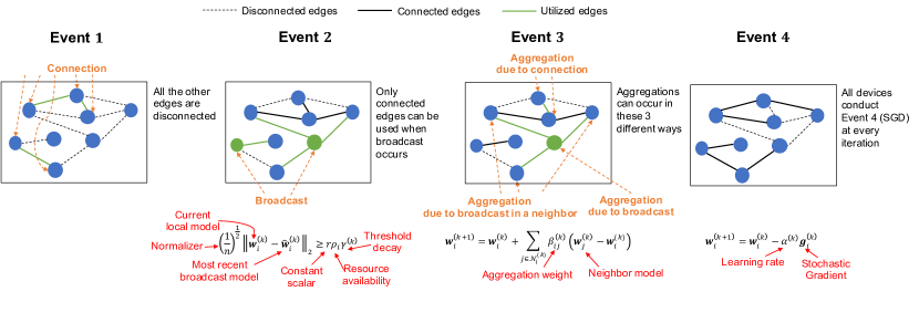
Figure 1: System diagram of a time-varying decentralized system, illustrating the four events of Alg. 1, namely (i) neighbor connection, (ii) model broadcast, (iii) model aggregation, and (iv) stochastic gradient descent.

In EF-HC, there are four types of events:

Event 1: Neighbor connection

The first event (lines 2-8 of Alg. 1) is triggered at device $i$ if new devices connect to it or existing devices disconnect from it due to the time-varying nature of the graph. Model parameters $\mathbf{w}_{i}^{(k)}$ and the degree of the device $i$ at that time $d_{i}^{(k)}$ are exchanged with this new neighbor. Consequently, this results in an aggregation event (Event 3) on both devices.

Event 2: Broadcast

If the normalized difference between $\mathbf{w}_{i}^{(k)}$ and $\mathbf{\widehat{w}}_{i}^{(k)}$ at device $i$ is greater than a threshold value $r\rho_{i}\gamma^{(k)}$, i.e.,

$${\left(\frac{1}{n}\right)}^{\frac{1}{2}}{\left\|\mathbf{w}_{i}^{(k)}-\mathbf{\widehat{w}}_{i}^{(k)}\right\|}_{2}\geq r\rho_{i}\gamma^{(k)},$$ (3)

then a broadcast event is triggered at that device (lines 9-13 of Alg. 1). In other words, communication at a device is triggered once the instantaneous local model is sufficiently different from the outdated one. When this event triggers, device $i$ broadcasts $\mathbf{w}_{i}^{(k)}$ and its degree $d_{i}^{(k)}$ to all its neighbors and receives the same information from them.

The threshold $r\rho_{i}\gamma^{(k)}$ is treated as heterogeneous across devices $i\in\mathcal{M}$, to assess whether the gain from a consensus iteration on the instantaneous main models at the devices will be worth the induced utilization of network resources. Specifically, (i) $r>0$ is a scaling hyperparameter value; (ii) $\gamma^{(k)}>0$ is a decaying factor that accounts for smaller expected variations in local models over time, and $\lim_{k\to\infty}{\gamma^{(k)}}=0$; and (iii) $\rho_{i}$ quantifies the availability of resources of device $i$. See [1] for some remarks on ${(\frac{1}{n})}^{\frac{1}{2}}$, $r$ and $\gamma^{(k)}$.

The development of ${(\frac{1}{n})}^{\frac{1}{2}}{\|\mathbf{w}_{i}^{(k)}-\mathbf{\widehat{w}}_{i}^{(k)}\|}_{2}$ and the condition $r\rho_{i}\gamma^{(k)}$ is one of our contributions relative to existing event-triggered schemes [35]. For example, in a bandwidth-limited environment, the transmission delay of the model transfer will be inversely proportional to the bandwidth among two devices. Thus, to decrease the latency of model training, $\rho_{i}$ can be defined inversely proportional to the bandwidth, promoting a lower frequency of communication on devices with less available bandwidth. In EF-HC, we set $\rho_{i}\propto\frac{1}{b_{i}}$, where $b_{i}$ is the average bandwidth on the outgoing links of the device $i$.

Event 3: Aggregation

Following a broadcast event (Event 2) or a neighbor connection event (Event 1) on device $i$, an aggregation event (lines 14-16 of Alg. 1) is triggered on device $i$ and all its neighbors. This aggregation is carried out through a distributed weighted averaging consensus method [19] as

$$\mathbf{w}_{i}^{(k+1)}=\mathbf{w}_{i}^{(k)}+\sum_{j\in\mathcal{N}^{\prime(k)}_{i}}{\beta_{ij}^{(k)}\left(\mathbf{w}_{j}^{(k)}-\mathbf{w}_{i}^{(k)}\right)},$$ (4)

where $\beta_{ij}^{(k)}$ is the aggregation weight that device $i$ assigns to parameters received from device $j$ in iteration $k$. The aggregation weights $\{\beta_{ij}^{(k)}\}$ for graph $\mathcal{G}^{(k)}$ can be selected based on the degree of neighbors, as will be discussed in Sec. III-B.

Event 4: Gradient descent

Each device $i$ conducts stochastic gradient descent (SGD) iterations for local model training (lines 17-18 of Alg. 1). Formally, device $i$ obtains $\mathbf{w}_{i}^{(k+1)}=\mathbf{w}_{i}^{(k)}-\alpha^{(k)}\mathbf{g}_{i}^{(k)}$, where $\alpha^{(k)}$ is the learning rate, and $\mathbf{g}_{i}^{(k)}$ is the stochastic gradient approximation defined as $\mathbf{g}_{i}^{(k)}=\frac{1}{|\mathcal{S}_{i}^{(k)}|}\sum_{\mathbf{\xi}\in\mathcal{S}_{i}^{(k)}}\nabla\ell_{\xi}{(\mathbf{w}_{i}^{(k)})}$. Here, $\mathcal{S}_{i}^{(k)}$ denotes the set of data points (mini-batch) used to compute the gradient, chosen uniformly at random from the local dataset. In our analysis, we define

$$\mathbf{g}_{i}^{(k)}=\nabla F_{i}{\left(\mathbf{w}_{i}^{(k)}\right)}+\mathbf{\epsilon}_{i}^{(k)},$$ (5)

in which $\nabla F_{i}{(\mathbf{w}_{i}^{(k)})}$ is the gradient of $F_{i}$ at $\mathbf{w}_{i}^{(k)}$, and $\mathbf{\epsilon}_{i}^{(k)}$ is the error due to the stochastic gradient approximation.

II-C Iterate Relations

We now express the model updates conducted in Alg. 1 in an iterative format, which will be useful in our subsequent theoretical analysis. Rewriting the event-based updates of Alg. 1 into one line of iterative model update, we get

$$\mathbf{w}_{i}^{(k+1)}=\mathbf{w}_{i}^{(k)}+\sum_{j\in\mathcal{N}^{\prime(k)}_{i}}{\beta_{ij}^{(k)}\left(\mathbf{w}_{j}^{(k)}-\mathbf{w}_{i}^{(k)}\right)v_{ij}^{(k)}}-\alpha^{(k)}\mathbf{g}_{i}^{(k)},$$ (6)

where $v_{ij}^{(k)}$ indicates whether device $i$ aggregates its model with device $j$ at iteration $k$. Its value depends on $v_{i}^{(k)}$, which is an indicator of a broadcast event at device $i$ at iteration $k$:

$$\begin{gathered}v_{i}^{(k)}=\begin{cases}1&{\left(\frac{1}{n}\right)}^{\frac{1}{2}}{\left\|\mathbf{w}_{i}^{(k)}-\mathbf{\widehat{w}}_{i}^{(k)}\right\|}_{2}>r\rho_{i}\gamma^{(k)}\\ 0&\text{o.w.}\end{cases},\\ \rho_{i}=\frac{1}{b_{i}},\qquad v_{ij}^{(k)}=\begin{cases}\max{\{v_{i}^{(k)},v_{j}^{(k)}\}}&j\in\mathcal{N}_{i}^{(k)}\\ 0&\text{o.w.}\end{cases}.\end{gathered}$$ (7)

Rearranging the relations in (6), we have

$$\mathbf{w}_{i}^{(k+1)}= \left(1-\sum_{j=1}^{m}{\beta_{ij}^{(k)}v_{ij}^{(k)}}\right)\mathbf{w}_{i}^{(k)}+\sum_{j=1}^{m}{\beta_{ij}^{(k)}v_{ij}^{(k)}\mathbf{w}_{j}^{(k)}}$$ (8)

$$-\alpha^{(k)}\mathbf{g}_{i}^{(k)}=\sum_{j=1}^{m}{p_{ij}^{(k)}\mathbf{w}_{j}^{(k)}}-\alpha^{(k)}\mathbf{g}_{i}^{(k)},$$

where $p_{ij}^{(k)}$ is the transition weight that device $i$ uses to aggregate device $j$’s parameters at iteration $k$

$$p_{ij}^{(k)}=\begin{cases}\beta_{ij}^{(k)}v_{ij}^{(k)}&\quad i\neq j\\ 1-\sum_{j=1}^{m}{\beta_{ij}^{(k)}v_{ij}^{(k)}}&\quad i=j\end{cases},$$ (9)

Next, we collect the parameter vectors of all devices that were previously introduced in matrix form as follows: $\mathbf{W}^{(k)}=\begin{bmatrix}\mathbf{w}_{1}^{(k)}&\cdots&\mathbf{w}_{m}^{(k)}\end{bmatrix}^{\top}$, $\mathbf{\widehat{W}}^{(k)}=\begin{bmatrix}\mathbf{\widehat{w}}_{1}^{(k)}&\cdots&\mathbf{\widehat{w}}_{m}^{(k)}\end{bmatrix}^{\top}$, $\mathbf{G}^{(k)}=\begin{bmatrix}\mathbf{g}_{1}^{(k)}&\cdots&\mathbf{g}_{m}^{(k)}\end{bmatrix}^{\top}$, $\mathbf{P}^{(k)}=[p_{ij}^{(k)}]_{1\leq i,j\leq m}$. Now, we transform the recursive update rules of (8) into matrix form to obtain the following relationship:

$$\mathbf{W}^{(k+1)}=\mathbf{P}^{(k)}\mathbf{W}^{(k)}-\alpha^{(k)}\mathbf{G}^{(k)}.$$ (10)

The recursive expression in (10) has been investigated before [13, 36]. However, the existing literature on decentralized stochastic gradient descent does not account for data heterogeneity, and this motivates us to use different analytical tools to derive convergence bounds.

As a conclusion to this section on iterate relations, we introduce two quantities, which will be frequently used in our analysis. We first derive an explicit relationship of (10). Starting from iteration $s$, where $s\leq k$, we have

$$\begin{gathered}\begin{aligned} \mathbf{W}^{(k+1)}=\mathbf{P}^{(k:s)}\mathbf{W}^{(s)}&-\sum_{r=s+1}^{k}{\alpha^{(r-1)}\mathbf{P}^{(k:r)}\mathbf{G}^{(r-1)}}\\ &-\alpha^{(k)}\mathbf{G}^{(k)},\end{aligned}\\ \mathbf{P}^{(k:s)}=\mathbf{P}^{(k)}\mathbf{P}^{(k-1)}\cdots\mathbf{P}^{(s+1)}\mathbf{P}^{(s)}.\end{gathered}$$ (11)

Second, to analyze the consensus of local models, we define the average model $\mathbf{\bar{w}}^{(k)}$ as

$$\mathbf{\bar{w}}^{(k)}=\frac{1}{m}\sum_{i=1}^{m}{\mathbf{w}_{i}^{(k)}}.$$ (12)

The recursive relation for $\mathbf{\bar{w}^{(k)}}$ using (8) and the stochasticity of $\mathbf{P}^{(k)}$ is

$$\mathbf{\bar{w}}^{(k+1)}=\mathbf{\bar{w}}^{(k)}-\frac{\alpha^{(k)}}{m}\sum_{i=1}^{m}{\mathbf{g}_{i}^{(k)}}.$$ (13)

Also, an explicit relationship between iteration $\mathbf{\bar{w}}^{(k+1)}$ and $\mathbf{\bar{w}}^{(s)}$, where $s\leq k$, easily follows from (13) as

$$\mathbf{\bar{w}}^{(k+1)}=\mathbf{\bar{w}}^{(s)}-\frac{1}{m}\sum_{r=s}^{k}{\alpha^{(r)}\sum_{i=1}^{m}{\mathbf{g}_{i}^{(r)}}}.$$ (14)

III Convergence Analysis

In this section, we first present our main theoretical contributions (Sec. III-A), and then detail the assumptions used to obtain them (Sec. III-B). Finally, we provide lemmas which are used to prove our main Theorems (Sec. III-C).

III-A Main Results

We first provide a proposition which demonstrates the information flow guarantees of our method, despite the devices conducting sporadic communications over a time-varying graph.

Proposition 1.

Let Assumption 8 hold. Under the EF-HC algorithm (Alg. 1), the information flow graph $\mathcal{G}^{\prime(k)}$ is $B$-connected, i.e., $\mathcal{G}^{\prime(k:k+B-1)}={(\mathcal{M},\cup_{s=0}^{B-1}{\mathcal{E}^{\prime(k+s)}})}$ is connected for any $k\geq 0$, where $B=(\tilde{l}+2)B_{1}$ and $\tilde{l}$ are determined via $\tilde{l}B_{1}\leq B_{2}\leq(\tilde{l}+1)B_{1}-1$. Note that $B_{1}$ and $B_{2}$ are, respectively, the connectivity bound of the physical network graph and the bound for the occurrence of communication events of Assumption 8-(a) and 8-(b).

Proof.

See Appendix A. ∎

It is important to note that we use $B$ only for convergence analysis, and it can have any arbitrarily large integer value. Therefore, we are not making strict connectivity assumptions on the underlying graph.

Finally, we obtain the convergence characteristics of EF-HC under the step size policies of Assumption 7. We reveal that using the diminishing step size of Assumption 7-(b), (a) all devices reach consensus asymptotically, i.e., each device $i$’s model $\mathbf{w}_{i}^{(k)}$ converges to $\mathbf{\bar{w}}^{(k)}=\frac{1}{m}\sum_{i=1}^{m}{\mathbf{w}_{i}^{(k)}}$ as $k\to\infty$, and (b) the final model across the devices (i.e., $\mathbf{\bar{w}}^{(k)},k\rightarrow\infty$) minimizes the global loss. By using the constant step size of assumption 7-(a), we also show that the same results for consensus and optimization hold but with an optimality gap which is proportional to the step size.

We further show that the convergence rate with a diminishing step size is $\mathcal{O}{\left(\frac{\ln{k}}{\sqrt{k}}\right)}$, which is a desirable property for decentralized gradient descent algorithms [34]:

Theorem 1.

Let the assumptions of Sec. III-B hold, and the constant step size policy of Assumption 7-(a) be used. Since using a constant step size will make $\mathbf{\Phi}^{(k)}$ and $\mathbf{\Psi}^{(k)}$ of (27) time-invariant, we denote these matrices as $\mathbf{\Phi}$ and $\mathbf{\Psi}$. If the step size $\alpha$ satisfies $\alpha\leq\frac{1-\rho^{2}}{4\sqrt{2}\sqrt{5-3\rho^{2}}BL{(1+\Gamma_{1})}^{B-1}}$, the following bound holds:

$$\begin{bmatrix}\mathbb{E}{\left[{\left\|\mathbf{\bar{w}}^{(kB)}-\mathbf{w}^{\star}\right\|}^{2}\right]}\\ \mathbb{E}{\left[{\left\|\mathbf{W}^{(kB)}-\mathbf{1}_{m}\mathbf{\bar{w}}^{(kB)}\right\|}^{2}\right]}\end{bmatrix}$$ (15)

$$\begin{aligned} \leq\mathcal{O}&{\left({\rho{\left(\mathbf{\Phi}\right)}}^{k}\right)}\begin{bmatrix}\mathbb{E}{\left[{\left\|\mathbf{\bar{w}}^{(0)}-\mathbf{w}^{\star}\right\|}^{2}\right]}\\ \mathbb{E}{\left[{\left\|\mathbf{W}^{(0)}-\mathbf{1}_{m}\mathbf{\bar{w}}^{(0)}\right\|}^{2}\right]}\end{bmatrix}\\ &+\left(\sum_{r=1}^{k-1}{\mathcal{O}{\left(\rho{\left(\mathbf{\Phi}\right)}^{k-r-1}\right)}}+1\right)\mathbf{\Psi}.\end{aligned}$$

Letting $k\to\infty$, we will get

$$\limsup_{k\to\infty} {\begin{bmatrix}\mathbb{E}{\left[{\left\|\mathbf{\bar{w}}^{(kB)}-\mathbf{w}^{\star}\right\|}^{2}\right]}\\ \mathbb{E}{\left[{\left\|\mathbf{W}^{(kB)}-\mathbf{1}_{m}\mathbf{\bar{w}}^{(kB)}\right\|}^{2}\right]}\end{bmatrix}}$$ (16)

$$\leq\frac{\alpha^{2}B}{\mathcal{O}{\left(1-\rho{\left(\mathbf{\Phi}\right)}\right)}}\begin{bmatrix}\frac{\sigma^{2}}{m}+\nu\\ 10mB\left\{\frac{\delta^{2}+2\mu\alpha\nu}{1-\rho^{2}}+2\sigma^{2}\right\}\end{bmatrix},$$

where

$$\nu=\frac{4}{\mu}\left(B-1\right)L^{2}{\left(1+\Gamma\right)}^{2\left(B-1\right)}\left(\frac{1+\Gamma}{2\sqrt{2}L}\delta^{2}+2\alpha\sigma^{2}\right).$$

Proof.

See Appendix F. ∎

This theorem indicates that, using a constant step size, linear convergence is achieved due to the term $\mathcal{O}{(\rho{(\mathbf{\Phi})}^{k})}$. However, we observe that using a constant step size will result in an asymptotic optimality gap of $\frac{\alpha^{2}}{\mathcal{O}{(1-\rho{(\mathbf{\Phi})})}}{\begin{bmatrix}\psi_{1},\psi_{2}\end{bmatrix}}^{\top}$. This gap is proportional to the step size $\alpha$ and the connectivity bound of the information flow graph $B$ (see Proposition 1). Thus, choosing a smaller $\alpha$ and employing a strategy that conducts communication rounds more frequently (decreasing $B$), results in the optimality gap getting smaller. On the other hand, the values of $\psi_{1}$ and $\psi_{2}$ depend on the data heterogeneity bound $\delta$, and the gradient approximation errors $\sigma$. This implies that in a federated setup where data distribution among devices are non-i.i.d., that is $\delta\neq 0$, the optimality gap cannot be made zero when a constant step size is employed, even if full gradients are used for the updates, i.e., $\sigma=0$.

First, we provide a supplementary lemma inspired by [37], which contains more generalizable results. We will later use this lemma in the proof of Theorem 2 in Appendix H.

Lemma 1.

Let ${\{\zeta_{r}\}}_{r=0}^{\infty}$ be a scalar sequence where $0<\zeta_{r}\leq 1$, $\forall r\geq 0$. For any $p\geq 1$, we have

$$\prod_{r=s}^{k}{{\left(1-\zeta_{r}\right)}^{p}}\leq\frac{1}{p\sum_{r=s}^{k}{\zeta_{r}}}.$$

Proof.

See Appendix G. ∎

Theorem 2.

Let the assumptions of Sec. III-B hold, and the diminishing step size policy of Assumption 7-(b) be used, with $\alpha^{(k)}=\frac{\alpha^{(0)}}{\sqrt{1+\nicefrac{{k}}{{\gamma}}}}$. If the step size satisfies $\alpha^{(0)}\leq\frac{1-\rho^{2}}{4\sqrt{2}\sqrt{5-3\rho^{2}}BL{(1+\Gamma_{1})}^{B-1}}$ where $\Gamma_{1}=\frac{1-\rho^{2}}{2\sqrt{5-3\rho^{2}}B}$, the following bound holds

$$\begin{bmatrix}\mathbb{E}{\left[{\left\|\mathbf{\bar{w}}^{(kB)}-\mathbf{w}^{\star}\right\|}^{2}\right]}\\ \mathbb{E}{\left[{\left\|\mathbf{W}^{(kB)}-\mathbf{1}_{m}\mathbf{\bar{w}}^{(kB)}\right\|}^{2}\right]}\end{bmatrix}$$ (17)

$$\begin{aligned} \leq\frac{1}{2\mu\alpha^{(0)}}\mathcal{O}{\left(\frac{1}{\sqrt{k}}\right)}&{\left(\frac{3+\rho^{2}}{4}\right)}^{K}\\ &\begin{bmatrix}\mathbb{E}{\left[{\left\|\mathbf{\bar{w}}^{(0)}-\mathbf{w}^{\star}\right\|}^{2}\right]}\\ \mathbb{E}{\left[{\left\|\mathbf{W}^{(0)}-\mathbf{1}_{m}\mathbf{\bar{w}}^{(0)}\right\|}^{2}\right]}\end{bmatrix}\end{aligned}$$

$$\begin{aligned} +\Bigg{\{}&\frac{1}{2\mu\alpha^{(0)}}\mathcal{O}{\left(\frac{1}{\sqrt{k}}\right)}\left(K-1\right)\left(\frac{1+\rho^{2}}{2}\right)\\ &+\frac{\alpha^{(0)}}{2}\mathcal{O}{\left(\frac{\ln{k}}{\sqrt{k}}\right)}+{(\alpha^{(0)})}^{2}\mathcal{O}{\left(\frac{1}{k}\right)}\Bigg{\}}B\begin{bmatrix}\widehat{\psi}_{1}\\ \widehat{\psi}_{2}\end{bmatrix},\end{aligned}$$

in which we have

$$\begin{gathered}\widehat{\psi}_{1}=\frac{\sigma^{2}}{m}+\nu^{(0)},\qquad\widehat{\psi}_{2}=10mB\left\{\frac{\delta^{2}+2\mu\alpha^{(0)}\nu^{(0)}}{1-\rho^{2}}+2\sigma^{2}\right\},\\ \nu^{(k)}=\frac{4}{\mu}\left(B-1\right)L^{2}{\left(1+\Gamma_{1}\right)}^{2\left(B-1\right)}\left(\frac{1+\Gamma_{1}}{2\sqrt{2}L}\delta^{2}+2\alpha^{(k)}\sigma^{2}\right).\end{gathered}$$

Letting $k\to\infty$, we will get

$$\limsup_{k\to\infty}{\begin{bmatrix}\mathbb{E}{\left[{\left\|\mathbf{\bar{w}}^{(kB)}-\mathbf{w}^{\star}\right\|}^{2}\right]}\\ \mathbb{E}{\left[{\left\|\mathbf{W}^{(kB)}-\mathbf{1}_{m}\mathbf{\bar{w}}^{(kB)}\right\|}^{2}\right]}\end{bmatrix}}=0.$$ (18)

Proof.

See Appendix H. ∎

Theorem 2 implies that using the diminishing step size of $\alpha^{(k)}=\frac{\alpha^{(0)}}{\sqrt{1+\nicefrac{{k}}{{\gamma}}}}$, a sub-linear rate of convergence $\frac{\ln{k}}{\sqrt{k}}$ can be achieved, and that the learning models of all devices asymptotically converge to the global optimum point. For the more general setup that the diminishing step size is chosen at $\alpha^{(k)}=\frac{\alpha^{(0)}}{{(1+\nicefrac{{k}}{{\gamma}})}^{\theta}}$ with $\theta\in(0.5,1]$, the results are provided in Appendix I.

It is worth mentioning that similar convergence rates have been shown in the literature [36], however, previous research derived this upper bound for a cumulative average of the model, $\frac{1}{T}\sum_{t=0}^{T-1}{\mathbf{w}^{(t)}}$, and not the model itself. Furthermore, the analysis of existing research was based on the (sub)gradient bound assumption [1], while we have replaced that with two more general assumptions, namely smoothness (Assumption 3) and statistical heterogeneity of data (Assumption 5).

III-B Assumptions for Main Results

In this section, we present all the assumptions used in our theoretical analysis.

Assumption 1 (Bidirectional Communication).

The devices exchange information simultaneously: if device $j$ communicates with device $i$ at some time, device $i$ also communicates with device $j$ at that same time.

Assumption 2 (Transition weights).

Let $\{p_{ij}^{(k)}\}$ be the set of aggregation weights in the information graph $\mathcal{G}^{\prime}(k)$. The following conditions must be met:

1. (Non-negative weights) $\forall i\in\mathcal{M}$, we have

   1. $p_{ii}^{(k)}>0$ and $p_{ij}^{(k)}>0$ for all $k\geq 0$ and all neighboring devices $j\in\mathcal{N}^{\prime(k)}_{i}$.

   2. $p_{ij}^{(k)}=0$, if $j\notin\mathcal{N}^{\prime(k)}_{i}$.

2. (Doubly-stochastic weights) The rows and columns of matrix $\mathbf{P}^{(k)}=[p_{ij}^{(k)}]$ are both stochastic, i.e., $\sum_{j=1}^{m}{p_{ij}^{(k)}}=1$, $\forall i$, and $\sum_{i=1}^{m}{p_{ij}^{(k)}}=1$, $\forall j$.

3. (Symmetric weights) $p_{ij}^{(k)}=p_{ji}^{(k)}$, $\forall i,k$ and $p_{ii}^{(k)}=1-\sum_{j\neq i}{p_{ij}^{(k)}}$.

Taking into account the conditions mentioned in Assumption 2, and the definition of $p_{ij}^{(k)}$ in (9), a choice of parameters $\beta_{ij}^{(k)}$ that satisfy these assumptions are as follows:

$$\beta_{ij}^{(k)}=\min{\left\{\frac{1}{1+d_{i}^{(k)}},\frac{1}{1+d_{j}^{(k)}}\right\}},$$ (19)

which is inspired by the Metropolis-Hastings algorithm [18]. Note that $p_{ij}^{(k)}$ also depends on $v_{ij}^{(k)}$, which was defined in (7).

Assumption 3 (Smoothness).

The local objective functions at each device $i$, i.e., $F_{i}$, has $L_{i}$-Lipschitz continuous gradients:

$$\left\|\nabla F_{i}{\left(\mathbf{w}\right)}-\nabla F_{i}{\left(\mathbf{w}^{\prime}\right)}\right\|\leq L_{i}\left\|\mathbf{w}-\mathbf{w}^{\prime}\right\|\leq L\left\|\mathbf{w}-\mathbf{w}^{\prime}\right\|,$$

where $L=\max_{i\in\mathcal{M}}{L_{i}}$.

Assumption 4 (Strong convexity).

The local objective function at each device $i$, i.e., $F_{i}$, is $\mu_{i}$-strongly convex:

$$\left\langle\nabla{F_{i}{\left(\mathbf{w}\right)}}-\nabla{F_{i}{\left(\mathbf{w}^{\prime}\right)}},\mathbf{w}-\mathbf{w}^{\prime}\right\rangle \geq\mu_{i}{\left\|\mathbf{w}-\mathbf{w}^{\prime}\right\|}^{2}$$

$$\geq\mu{\left\|\mathbf{w}-\mathbf{w}^{\prime}\right\|}^{2},$$

$\forall(\mathbf{{w}^{\prime}},\mathbf{w})\in\mathbb{R}^{n}\times\mathbb{R}^{n}$, in which $\mu=\min_{i\in\mathcal{M}}{\mu_{i}}$.

Note that the global objective function $F{(\mathbf{w})}$, which is a convex combination of local objective functions, will also be strongly convex, thus having a unique minimizer, denoted by $\mathbf{w}^{\star}=\operatorname*{arg\,min}_{\mathbf{w}\in\mathbb{R}^{n}}{F{(\mathbf{w})}}$. Additionally, following Assumptions 3 and 4, we have $\mu\leq\mu_{i}\leq L_{i}\leq L$, for all $i\in\mathcal{M}$.

Inspired by [7, 34], we make the following assumption about the heterogeneity of the data.

Assumption 5 (Data heterogeneity).

The data heterogeneity across the devices is measured via $\delta_{i}>0$ as

$$\left\|\nabla F_{i}{\left(\mathbf{w}\right)}-\nabla F{\left(\mathbf{w}\right)}\right\|\leq\delta_{i}\leq\delta,$$

for all $\mathbf{w}\in\mathbb{R}^{n}$ and all $i\in\mathcal{M}$, in which $\delta=\max_{i\in\mathcal{M}}{\delta_{i}}$.

Assumption 6 (Gradient approximation errors).

We make the following assumptions on the gradient approximation errors $\mathbf{\epsilon}_{i}^{(k)}$ for all $i\in\mathcal{M}$ and all $k\geq 0$:

1. Zero mean, i.e., ${\|\mathbb{E}{[\mathbf{\epsilon}_{i}^{(k)}]}\|}_{2}=0$ .

2. Bounded mean square, i.e., there are scalars $\sigma_{i}^{2}$ such that $\mathbb{E}{[{\|\mathbf{\epsilon}_{i}^{(k)}\|}_{2}^{2}]}\leq\sigma_{i}^{2}\leq\sigma^{2}$, where $\sigma=\max_{i\in\mathcal{M}}{\sigma_{i}}$.

3. Each random vector $\epsilon_{i}^{(k)}$ is independent from $\epsilon_{j}^{(k)}$ for all $i\in\mathcal{M}$, $j\neq i$.

Assumption 7 (Step sizes).

All devices use the same step size for model training. We study the behavior of our algorithm under two policies for the step size:

1. Constant step size, having $\alpha^{(k)}=\alpha$ where $\alpha>0$.

2. Diminishing step size, in which the step size decays over time, satisfying the following conditions.

   $$\lim_{k\to\infty}{\alpha^{(k)}}=0,\quad\sum_{k=0}^{\infty}{\alpha^{(k)}}=\infty,\quad\sum_{k=0}^{\infty}{{\left(\alpha^{(k)}\right)}}^{2}<\infty.$$

In particular, setting $\alpha^{(k)}=\frac{\alpha^{(0)}}{{(1+\nicefrac{{k}}{{\gamma}})}^{\theta}}$ meets the criteria of Assumption 7-(b) for $\alpha^{(0)},\gamma>0$, and $\theta\in(0.5,1]$.

The previous assumptions are common in the literature [7, 11]. In the next assumption, we introduce a relaxed version of graph connectivity requirements relative to existing work in distributed learning, which underscores the difference of our decentralized event-triggered FL method compared with traditional distributed optimization algorithms.

Assumption 8 (Network graph connectivity).

The underlying communication graph satisfies the following properties:

1. There exists an integer $B_{1}\geq 1$ such that the graph union of the physical network graph $\mathcal{G}^{(k)}=(\mathcal{M},\mathcal{E}^{(k)})$ from any arbitrary iteration $k$ to $k+B_{1}-1$, i.e., $\mathcal{G}^{(k:k+B_{1}-1)}={(\mathcal{M},\cup_{s=0}^{B_{1}-1}{\mathcal{E}^{(k+s)}})}$, is connected for any $k\geq 0$.

2. There exists an integer $B_{2}\geq 1$ such that for every device $i$, triggering conditions for the broadcast event occur at least once every $B_{2}$ consecutive iterations $\forall k\geq 0$. This is equivalent to the following condition:

   $$\exists B_{2}\geq 1,\forall i:\max{\{v_{i}^{(k)},v_{i}^{(k+1)},\cdots,v_{i}^{(k+B_{2}-1)}\}}=1.$$

Using the above assumption, we show the connectivity behavior of information flow graphs, i.e., $\mathcal{G}^{\prime(k)}$, in Proposition 1.

III-C Intermediate Lemmas for Main Results

In this section, we provide some lemmas which are useful in the proofs of Theorems 1 and 2. These lemmas also provide additional characteristics of our methodology.

Our first lemma gives a bound on $\|\mathbf{P}^{(k:s)}\mathbf{W}^{(k)}-\mathbf{1}_{m}\mathbf{\bar{w}}^{(k)}\|$ using the spectral norm of $\mathbf{P}^{(k:s)}$, which we show that depending on iteration $s$, this bound can be made tighter.

Lemma 2 (Follows from Sec. II-B of [38]).

Let Assumption 2 hold, and let $B$ be the connectivity bound of Proposition 1. Then the following is true

1. From iteration $k$ to $k+B-r$, where $r=2,\cdots,B$, we have

   $$\left\|\mathbf{P}^{(k+B-r:k)}\mathbf{W}^{(k)}-\mathbf{1}_{m}\mathbf{\bar{w}}^{(k)}\right\|$$

   $$\leq\rho^{(k+B-r:k)}\left\|\mathbf{W}^{(k)}-\mathbf{1}_{m}\mathbf{\bar{w}}^{(k)}\right\|\leq\left\|\mathbf{W}^{(k)}-\mathbf{1}_{m}\mathbf{\bar{w}}^{(k)}\right\|.$$

2. From iteration $k$ to $k+B-1$, we have the following.

   $$\left\|\mathbf{P}^{(k+B-1:k)}\mathbf{W}^{(k)}-\mathbf{1}_{m}\mathbf{\bar{w}}^{(k)}\right\|$$

   $$\leq\rho^{(k+B-1:k)}\left\|\mathbf{W}^{(k)}-\mathbf{1}_{m}\mathbf{\bar{w}}^{(k)}\right\|\leq\rho\left\|\mathbf{W}^{(k)}-\mathbf{1}_{m}\mathbf{\bar{w}}^{(k)}\right\|,$$

   in which $\rho^{(k+B-r:k)}=\rho{(\mathbf{P}^{(k+B-r:k)})}$, $\rho=\sup_{k=0,1,\cdots}{\rho{(\mathbf{P}^{(k+B-1:k)})}}$, and $0<\rho<1$.

Proof.

Since the graph is time-varying, we can only guarantee the connectivity of $0<\mathbf{P}^{(k+B-1:k)}$. Therefore, $0<\rho{(\mathbf{P}^{(k+B-r:k)})}\leq 1$ for all $r=2,\cdots,B$, but $0<\rho<1$. The rest of the proof follows from Sec. II-B of [38]. ∎

Lemma 2 is essential in the analysis of our method and helps us to prove the convergence under time-varying communication graphs with an arbitrary connectivity bound.

Definition 1.

We define the following gradient matrices: $\mathbf{\nabla}^{(k)}={\begin{bmatrix}\nabla{F_{1}{(\mathbf{w}_{i}^{(k)})}},\cdots,\nabla{F_{m}{(\mathbf{w}_{m}^{(k)})}}\end{bmatrix}}^{\top}$, $\mathbf{\bar{\nabla}}^{(k)}=\frac{1}{m}\mathbf{1}_{m}^{\top}\mathbf{\nabla}^{(k)}$ and $\mathbf{\nabla}{F}^{(k)}={\begin{bmatrix}\nabla{F{(\mathbf{w}_{i}^{(k)})}},\cdots,\nabla{F{(\mathbf{w}_{m}^{(k)})}}\end{bmatrix}}^{\top}$. Furthermore, note that $\nabla{F{(\mathbf{\bar{w}}^{(k)})}}\in\mathbb{R}^{1\times n}$, is the gradient of global objective function evaluated at $\mathbf{\bar{w}}^{(k)}$.

Using the previous definition, we next provide two inequalities which help us bound the expressions involving the gradients in any iteration $k$, via the values of the model parameters, scaled by a constant factor.

Lemma 3 (Follows from Lemmas 8-(c) and 10 of [38]).

Under Assumptions 3 and 4, the following holds for all $k\geq 0$:

$$\left\|\nabla{F{\left(\mathbf{\bar{w}}^{(k)}\right)}}-\mathbf{\bar{\nabla}}^{(k)}\right\|\leq\frac{L}{\sqrt{m}}\left\|\mathbf{W}^{(k)}-\mathbf{1}_{m}\mathbf{\bar{w}}^{(k)}\right\|.$$

Also, if $\alpha^{(k)}<\frac{2}{\mu+L}$, then

$$\Big{\|}\mathbf{\bar{w}}^{(k)}-\alpha^{(k)}\nabla{F{\left(\mathbf{\bar{w}}^{(k)}\right)}}-\mathbf{w}^{\star}\Big{\|}\leq\left(1-\mu\alpha^{(k)}\right)\left\|\mathbf{\bar{w}}^{(k)}-\mathbf{w}^{\star}\right\|.$$

Next, we obtain the following bounds for the average of gradient approximation errors, which are used to obtain the results of several subsequent lemmas.

Lemma 4.

Let Assumption 6 hold. Provided the definitions $\mathbf{\bar{\epsilon}}^{(k)}=\frac{1}{m}\sum_{i=1}^{m}{\mathbf{\epsilon}_{i}^{(k)}}$ and $\mathbf{\epsilon}^{(k)}={\begin{bmatrix}\mathbf{\epsilon}_{1}^{(k)},\cdots,\mathbf{\epsilon}_{m}^{(k)}\end{bmatrix}}^{\top}$, we have

$$\begin{gathered}\mathbb{E}{\left[{\left\|\mathbf{\bar{\epsilon}}^{(k)}\right\|}^{2}\right]}\leq\frac{\sigma^{2}}{m},\quad\mathbb{E}{\left[{\left\|\mathbf{\epsilon}^{(k)}-\mathbf{1}_{m}\mathbf{\bar{\epsilon}}^{(k)}\right\|}^{2}\right]}\leq 4m\sigma^{2}.\end{gathered}$$

Proof.

The first inequality follows from Lemma 2 of [15]. For the proof of the second bound, see Appendix B. ∎

Traditional analysis of distributed gradient descent involves making the assumption of bounded gradient (see [13], [14]). However, since we have replaced such an assumption with two different but more general assumptions, namely smoothness and data heterogeneity (Assumptions 3 and 5), our analysis is different compared to the current literature. Inspired by the gradient tracking literature in distributed learning [38, 15], in the following lemma, we look at the behavior of ${\|\mathbf{W}^{(k+1)}-\mathbf{1}_{m}\mathbf{\bar{w}}^{(k+1)}\|}^{2}$ and ${\|\mathbf{\bar{w}}^{(k+1)}-\mathbf{w}^{\star}\|}^{2}$, and bound them simultaneously via a system of inequalities.

Lemma 5.

Assumptions 3-6 yield the following bounds:

1. Consensus error on local gradients:

   $${\left\|\mathbf{\nabla}^{(k)}-\mathbf{1}_{m}\mathbf{\bar{\nabla}}^{(k)}\right\|}^{2}\leq 2m\delta^{2}+8L^{2}{\left\|\mathbf{W}^{(k)}-\mathbf{1}_{m}\mathbf{\bar{w}}^{(k)}\right\|}^{2}.$$

2. Assuming $\alpha^{(k)}<\frac{2}{\mu+L}$, the optimization error:

   $$\mathbb{E} {\left[{\left\|\mathbf{\bar{w}}^{(k+1)}-\mathbf{w}^{\star}\right\|}^{2}\right]}\leq\left(1-\mu\alpha^{(k)}\right)\mathbb{E}{\left[{\left\|\mathbf{\bar{w}}^{(k)}-\mathbf{w}^{\star}\right\|}^{2}\right]}$$

   $$+\left(1+\mu\alpha^{(k)}\right)\frac{\alpha^{(k)}L^{2}}{\mu m}\mathbb{E}{\left[{\left\|\mathbf{W}^{(k)}-\mathbf{1}_{m}\mathbf{\bar{w}}^{(k)}\right\|}^{2}\right]}$$

   $$+\frac{{\left(\alpha^{(k)}\right)}^{2}\sigma^{2}}{m}.$$

3. Expected consensus error of model weights:

   $$\mathbb{E} {\left[{\left\|\mathbf{W}^{(k+1)}-\mathbf{1}_{m}\mathbf{\bar{w}}^{(k+1)}\right\|}^{2}\right]}\leq$$

   $${\left(1+2\sqrt{2}\alpha^{(k)}L\right)}^{2}\mathbb{E}{\left[{\left\|\mathbf{W}^{(k)}-\mathbf{1}_{m}\mathbf{\bar{w}}^{(k)}\right\|}^{2}\right]}$$

   $$+2m{\left(\alpha^{(k)}\right)}^{2}\left[\frac{1+2\sqrt{2}\alpha^{(k)}L}{2\sqrt{2}\alpha^{(k)}L}\delta^{2}+2\sigma^{2}\right].$$

Proof.

See Appendix C. ∎

We make two observations from the above lemma. First, consider the term $2m\delta^{2}$ in Lemma 5-(a). This term reveals that even if consensus is reached among the devices, i.e., ${\|\mathbf{W}^{(k)}-\mathbf{1}_{m}\mathbf{\bar{w}}^{(k)}\|}^{2}=0$, the local gradients would always be different from each other due to the data heterogeneity assumption of 5. Second, the system of inequalities is semi-coupled, as we can bound ${\|\mathbf{W}^{(k+1)}-\mathbf{1}_{m}\mathbf{\bar{w}}^{(k)}\|}^{2}$ at each iteration only by its own value at the previous iterations.

Next, we write the iterate relations defined in parts (c)&(b) of Lemma 5 as a system of recursive inequalities:

$$\begin{bmatrix}\mathbb{E}{\left[{\left\|\mathbf{\bar{w}}^{(k+1)}-\mathbf{w}^{\star}\right\|}^{2}\right]}\\ \mathbb{E}{\left[{\left\|\mathbf{W}^{(k+1)}-\mathbf{1}_{m}\mathbf{\bar{w}}^{(k+1)}\right\|}^{2}\right]}\end{bmatrix}$$ (20)

$$\leq\mathbf{A}^{(k)}\begin{bmatrix}\mathbb{E}{\left[{\left\|\mathbf{\bar{w}}^{(k)}-\mathbf{w}^{\star}\right\|}^{2}\right]}\\ \mathbb{E}{\left[{\left\|\mathbf{W}^{(k)}-\mathbf{1}_{m}\mathbf{\bar{w}}^{(k)}\right\|}^{2}\right]}\end{bmatrix}+\mathbf{C}^{(k)},$$

in which $\mathbf{A}^{(k)}={[a_{ij}^{(k)}]}_{1\leq i,j\leq 2}$ and $\mathbf{C}^{(k)}={[c_{1}^{(k)},c_{2}^{(k)}]}^{\top}$. and

$$a_{11}^{(k)}=1-\mu\alpha^{(k)},\quad a_{12}^{(k)}=\left(1+\mu\alpha^{(k)}\right)\frac{\alpha^{(k)}L^{2}}{\mu m},$$ (21)

$$a_{21}^{(k)}=0,\quad a_{22}^{(k)}={\left(1+2\sqrt{2}\alpha^{(k)}L\right)}^{2},$$

$$c_{1}^{(k)}=\frac{{\left(\alpha^{(k)}\right)}^{2}\sigma^{2}}{m},$$

$$c_{2}^{(k)}=2m{\left(\alpha^{(k)}\right)}^{2}\left(\frac{1+2\sqrt{2}\alpha^{(k)}L}{2\sqrt{2}\alpha^{(k)}L}\delta^{2}+2\sigma^{2}\right).$$

Next, we derive an explicit relation for the system of inequalities of (20), starting from an arbitrary iteration $s$ as

$$\begin{bmatrix}\mathbb{E}{\left[{\left\|\mathbf{\bar{w}}^{(k+1)}-\mathbf{w}^{\star}\right\|}^{2}\right]}\\ \mathbb{E}{\left[{\left\|\mathbf{W}^{(k+1)}-\mathbf{1}_{m}\mathbf{\bar{w}}^{(k+1)}\right\|}^{2}\right]}\end{bmatrix}$$ (22)

$$\leq\mathbf{A}^{(k:s)}\begin{bmatrix}\mathbb{E}{\left[{\left\|\mathbf{\bar{w}}^{(s)}-\mathbf{w}^{\star}\right\|}^{2}\right]}\\ \mathbb{E}{\left[{\left\|\mathbf{W}^{(s)}-\mathbf{1}_{m}\mathbf{\bar{w}}^{(s)}\right\|}^{2}\right]}\end{bmatrix}$$

$$+\sum_{r=s+1}^{k}{\mathbf{A}^{(k:r)}\mathbf{C}^{(r-1)}}+\mathbf{C}^{(k)},$$

in which $\mathbf{A}^{(k:s)}=\mathbf{A}^{(k)}\cdots\mathbf{A}^{(s)}$. Since $a_{21}^{(k)}=0$, we can easily compute the following entries of $\mathbf{A}^{(k:s)}$ which will be frequently used in our analysis:

$$a_{11}^{(k:s)}=a_{11}^{(k)}\cdots a_{11}^{(s)},a_{21}^{(k:s)}=0,a_{22}^{(k:s)}=a_{22}^{(k)}.\cdots a_{22}^{(s)}.$$ (23)

As mentioned before Lemma 5, similar analysis to our paper is common in the gradient tracking literature. But current research has only shown convergence guarantees over static communication graphs. Next, we move on to an important lemma of our paper, which is the key to proving the convergence for time-varying graphs with arbitrary connectivity $B$.

Lemma 6.

Using Lemma 5, Assumptions 3, 4, 5 and 6, we can get the following inequality on the expected consensus error of the model weights at iteration $k+B$ for any $k\geq 0$:

$$\mathbb{E}{\left[{\left\|\mathbf{W}^{(k+B)}-\mathbf{1}_{m}\mathbf{\bar{w}}^{(k+B)}\right\|}^{2}\right]}$$

$$\begin{aligned} \leq\,\,&\left[\frac{1+\rho^{2}}{2}+8\frac{5-3\rho^{2}}{1-\rho^{2}}BL^{2}\sum_{r=k+1}^{k+B}{\left(\alpha^{(r-1)}\right)}^{2}a_{22}^{(r-2:k)}\right]\\ &\mathbb{E}{\left[{\left\|\mathbf{W}^{(k)}-\mathbf{1}_{m}\mathbf{\bar{w}}^{(k)}\right\|}^{2}\right]}+2\frac{5-3\rho^{2}}{1-\rho^{2}}B\sum_{r=k+1}^{k+B}{\left(\alpha^{(r-1)}\right)}^{2}\\ &\left[m\delta^{2}+4L^{2}\left(\sum_{l=k+1}^{r-2}{a_{22}^{(r-2:l)}c_{2}^{(l-1)}}+c_{2}^{(r-2)}\right)\right]\\ &+20mB\sigma^{2}\sum_{r=k+1}^{k+B}{{\left(\alpha^{(r-1)}\right)}^{2}},\end{aligned}$$

where $0<\rho^{(k+B-1:k)}\leq\rho<1$ for any $k\geq 0$, and $B$ is the connectivity bound of 1.

Proof.

See Appendix D. ∎

We next derive a system of inequalities for the iterate relations of Lemma 5-(c)&(b), but instead of writing a recursive relation between iteration $k+1$ and $k$ as in (20), we use Lemma 6 to obtain a recursive relation between $k+B$ and $k$:

$$\begin{bmatrix}\mathbb{E}{\left[{\left\|\mathbf{\bar{w}}^{(\left(k+1\right)B)}-\mathbf{w}^{\star}\right\|}^{2}\right]}\\ \mathbb{E}{\left[{\left\|\mathbf{W}^{(\left(k+1\right)B)}-\mathbf{1}_{m}\mathbf{\bar{w}}^{(\left(k+1\right)B)}\right\|}^{2}\right]}\end{bmatrix}$$ (24)

$$\leq\mathbf{\Phi}^{(k)}\begin{bmatrix}\mathbb{E}{\left[{\left\|\mathbf{\bar{w}}^{(kB)}-\mathbf{w}^{\star}\right\|}^{2}\right]}\\ \mathbb{E}{\left[{\left\|\mathbf{W}^{(kB)}-\mathbf{1}_{m}\mathbf{\bar{w}}^{(kB)}\right\|}^{2}\right]}\end{bmatrix}+\mathbf{\Psi}^{(k)},$$

in which $\mathbf{\Phi}^{(k)}={[\phi_{ij}^{(k)}]}_{1\leq i,j\leq 2}$, and $\mathbf{\Psi}^{(k)}={[\psi_{1}^{(k)},\psi_{2}^{(k)}]}^{\top}$, and

$$\phi_{11}^{(k)}=a_{11}^{(\left(k+1\right)B-1:kB)},\quad\phi_{12}^{(k)}=a_{12}^{(\left(k+1\right)B-1:kB)},$$ (25)

$$\phi_{21}^{(k)}=0,$$

$$\phi_{22}^{(k)}=\frac{1+\rho^{2}}{2}+8\frac{5-3\rho^{2}}{1-\rho^{2}}BL^{2}\sum_{r=kB+1}^{\left(k+1\right)B}{\left(\alpha^{(r-1)}\right)}^{2}a_{22}^{(r-2:k)},$$

$$\begin{aligned} \psi_{1}^{(k)}=\,\,&\sum_{r=kB+1}^{\left(k+1\right)B-1}{\left(\alpha^{(r-1)}\right)}^{2}\Bigg{[}a_{11}^{(\left(k+1\right)B-1:r)}\frac{\sigma^{2}}{m}\\ &+2ma_{12}^{(\left(k+1\right)B-1:r)}\left(\frac{1+2\sqrt{2}\alpha^{(r-1)}L}{2\sqrt{2}\alpha^{(r-1)}L}\delta^{2}+2\sigma^{2}\right)\Bigg{]}\\ &+\frac{{\left(\alpha^{(\left(k+1\right)B-1)}\right)}^{2}\sigma^{2}}{m},\end{aligned}$$ (26)

$$\begin{aligned} \psi_{2}^{(k)}&=2B\sum_{r=kB+1}^{\left(k+1\right)B}{\left(\alpha^{(r-1)}\right)}^{2}\Bigg{\{}\frac{5-3\rho^{2}}{1-\rho^{2}}\Bigg{[}m\delta^{2}\\ &+4L^{2}\Bigg{(}\sum_{l=kB+1}^{r-2}{a_{22}^{(r-2:l)}c_{2}^{(l-1)}}+c_{2}^{(r-2)}\Bigg{)}\Bigg{]}+10m\sigma^{2}\Bigg{\}}.\end{aligned}$$

Comparing (22) and (24), note that we have used $\mathbf{\Phi}^{(k)}=\mathbf{A}^{((k+1)B-1:kB)}$ and $\mathbf{\Psi}^{(k)}=\sum_{r=kB+1}^{(k+1)B-1}{\mathbf{A}^{((k+1)B-1:r)}\mathbf{C}^{(r-1)}}+\mathbf{C}^{((k+1)B-1)}$, except for two modifications, where we have replaced $\phi_{22}^{(k)}$ and $\psi_{2}^{(k)}$ with the values derived in Lemma 6.

Next, we derive an explicit equation for the system of inequalities of (24), starting from an arbitrary iteration $s$, as follows.

$$\begin{bmatrix}\mathbb{E}{\left[{\left\|\mathbf{\bar{w}}^{(\left(k+1\right)B)}-\mathbf{w}^{\star}\right\|}^{2}\right]}\\ \mathbb{E}{\left[{\left\|\mathbf{W}^{(\left(k+1\right)B)}-\mathbf{1}_{m}\mathbf{\bar{w}}^{(\left(k+1\right)B)}\right\|}^{2}\right]}\end{bmatrix}$$ (27)

$$\leq\mathbf{\Phi}^{(k:s)}\begin{bmatrix}\mathbb{E}{\left[{\left\|\mathbf{\bar{w}}^{(sB)}-\mathbf{w}^{\star}\right\|}^{2}\right]}\\ \mathbb{E}{\left[{\left\|\mathbf{W}^{(sB)}-\mathbf{1}_{m}\mathbf{\bar{w}}^{(sB)}\right\|}^{2}\right]}\end{bmatrix}$$

$$+\sum_{r=s+1}^{k}{\mathbf{\Phi}^{(k:r)}\mathbf{\Psi}^{(r-1)}}+\mathbf{\Psi}^{(k)},$$

in which $\mathbf{\Phi}^{(k:s)}=\mathbf{\Phi}^{(k)}\cdots\mathbf{\Phi}^{(s)}$. Since $\phi_{21}^{(k)}=0$ (see (25)), we can easily compute the following entries of $\mathbf{\Phi}^{(k:s)}$ that will be used in our analysis.

$$phi_{11}^{(k:s)}=\phi_{11}^{(k)}\cdots\phi_{11}^{(s)},\phi_{21}^{(k:s)}=0,\quad\phi_{22}^{(k:s)}=\phi_{22}^{(k)}.\cdots\phi_{22}^{(s)}.$$ (28)

In the subsequent proposition, we build on the results of equation (27), and obtain the conditions under which the spectral norm of $\mathbf{\Phi}^{(k)}$ would be less than one. Then, we use that to bound the system of inequalities of (27).

Proposition 2.

Let the assumptions of Sec. III-B hold, and a non-increasing step size be used such that $\alpha^{(k+1)}\leq\alpha^{(k)}$ for all $k\geq 0$ . Using the definitions of $\mathbf{\Phi}^{(k:s)}$ and $\mathbf{\Psi}^{(k:s)}$ in (27), if the step size satisfies $\alpha^{(0)}\leq\frac{1-\rho^{2}}{4\sqrt{2}\sqrt{5-3\rho^{2}}BL{(1+\Gamma_{1})}^{B-1}}$ where $\Gamma_{1}=\frac{1-\rho^{2}}{2\sqrt{5-3\rho^{2}}B}$, the following bound holds

$$\begin{bmatrix}\mathbb{E}{\left[{\left\|\mathbf{\bar{w}}^{(kB)}-\mathbf{w}^{\star}\right\|}^{2}\right]}\\ \mathbb{E}{\left[{\left\|\mathbf{W}^{(kB)}-\mathbf{1}_{m}\mathbf{\bar{w}}^{(kB)}\right\|}^{2}\right]}\end{bmatrix}$$ (29)

$$\begin{aligned} \leq\mathcal{O}&{\left(\phi_{11}^{(k-1:K)}\right)}\mathcal{O}{\left(\phi_{22}^{(K-1:0)}\right)}\begin{bmatrix}\mathbb{E}{\left[{\left\|\mathbf{\bar{w}}^{(0)}-\mathbf{w}^{\star}\right\|}^{2}\right]}\\ \mathbb{E}{\left[{\left\|\mathbf{W}^{(0)}-\mathbf{1}_{m}\mathbf{\bar{w}}^{(0)}\right\|}^{2}\right]}\end{bmatrix}\end{aligned}$$

$$+\mathcal{O}{\left(\phi_{11}^{(k-1:K)}\right)}\sum_{r=1}^{K-1}{\mathcal{O}{\left(\phi_{22}^{(K-1:r)}\right)}\mathbf{\Psi}^{(r-1)}}$$

$$+\sum_{r=K}^{k-1}{\mathcal{O}{\left(\phi_{11}^{(k-1:r)}\right)}\mathbf{\Psi}^{(r-1)}}+\mathbf{\Psi}^{(k-1)},$$

where iteration $K$ is determined by $\phi_{11}^{(k)}<\phi_{22}^{(k)}$ for all $k=0,\cdots,K-1$, and $\phi_{11}^{(k)}\geq\phi_{22}^{(k)}$ for $k\geq K$.

Furthermore, the matrix $\mathbf{\Psi}^{(k)}$ can be bounded as

$$\mathbf{\Psi}^{(k)}\leq{\left(\alpha^{(kB)}\right)}^{2}B\begin{bmatrix}\left\{\frac{\sigma^{2}}{m}+\nu^{(kB)}\right\}\\ 10mB\left\{\frac{\delta^{2}+2\mu\alpha^{(kB)}\nu^{(kB)}}{1-\rho^{2}}+2\sigma^{2}\right\}\end{bmatrix},$$ (30)

where

$$\nu^{(k)}=\frac{4}{\mu}\left(B-1\right)L^{2}{\left(1+\Gamma_{1}\right)}^{2\left(B-1\right)}\left(\frac{1+\Gamma_{1}}{2\sqrt{2}L}\delta^{2}+2\alpha^{(k)}\sigma^{2}\right).$$

Proof.

See Appendix E. ∎

The above result implies that if the spectral norm of $\mathbf{\Phi}^{(k)}$ satisfies $\rho{(\mathbf{\Phi}^{(k)})}=\max{\{\phi_{11}^{(k)},\phi_{22}^{(k)}\}}<1$, then we can bound the system of inequalities in terms of the spectral norm. Moreover, the matrix $\mathbf{\Phi}^{(k-1:0)}$ is separated into the product of two terms $\mathbf{\Phi}^{(k-1:K)}\mathbf{\Phi}^{(K-1:0)}$, and this is done because we have $\rho{(\mathbf{\Phi}^{(K-1:0)})}=\phi_{22}^{(K-1:0)}$ and $\rho{(\mathbf{\Phi}^{(k-1:K-1)})}=\phi_{11}^{(k-1:K-1)}$ (see Appendix E for more discussion). This lemma is directly used to prove Theorems 1 and 2.

Next, we analyze the dependence of the constraint over $\alpha^{(0)}$ on $B$, as we show that it is inversely proportional to $B$. The reason we emphasize this point is that in subsequent theoretical analysis, we will upper-bound $\Gamma_{1}$ with $\frac{1}{2\sqrt{2}}$, obtaining a relationship $\alpha^{(0)}\propto\frac{1}{B{(1+\frac{1}{2\sqrt{2}})}^{B-1}}$, but this does not imply an inversely exponential dependence of $\alpha^{(0)}$ on $B$. We have

$$\alpha^{(0)} \leq\mathcal{O}{\left(\frac{1}{B{\left(1+\Gamma_{1}\right)}^{B-1}}\right)}=\mathcal{O}{\left(\frac{1}{B{\left(1+\frac{1-\rho^{2}}{2\sqrt{5-3\rho^{2}}B}\right)}^{B-1}}\right)}$$

$$=\mathcal{O}{\left(\frac{1}{B{\left(1+\frac{1}{B}\right)}^{B}}\right)}=\mathcal{O}{\left(\frac{1}{B}\right)}.$$

IV Numerical Results

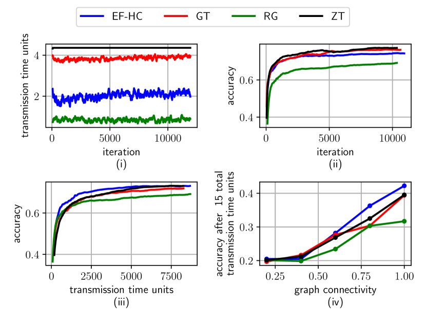
(a) Fashion-MNIST data set

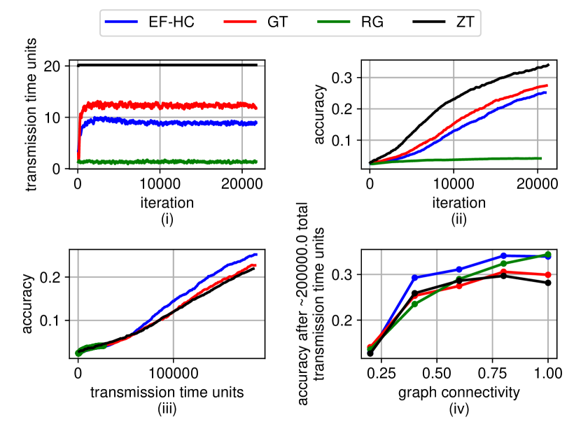
(b) Federated Extended MNIST data set

Figure 2: Performance comparison between our method (EF-HC), global threshold (GT), zero threshold (ZT), and randomized gossip (RG) algorithms. The plots show (i) transmission time per iteration, (ii) accuracy per iteration, (iii) accuracy per transmission time, and (iv) accuracy after a certain number of transmissions with respect to graph connectivity.

In this section, we present the outcomes of our numerical simulations, which validate the effectiveness of our methodology. We explain the setup of our experiments in Sec. IV-A and provide the results and discussion in Sec. IV-B.

IV-A Simulation Setup

We evaluate our proposed methodology using two image classification tasks: Fashion-MNIST (FMNIST) [39], and Federated Extended MNIST (FEMNIST) [40]. Note that FMNIST contains data belonging to $10$ labels, while FEMNIST contains data points with $62$ different labels. We employ the support vector machine (SVM) as the classifier, which satisfies the convexity assumption (see 4). The loss function $\ell_{\xi}{(\mathbf{w})}$ in (1) is chosen as the multi-margin loss for the SVM model. Supplementary experimental results for a non-convex deep learning model are given in Appendix J.

In the simulations for the FMNIST and FEMNIST data sets, a network of devices $m=10$ and $m=30$ is used, respectively, in which the underlying communications topology is generated as a random geometric graph with connectivity $0.4$ [11]. To generate non-i.i.d. data distributions across devices, each device only contains samples of the data set from a subset of the labels. For FMNIST and FEMNIST, we consider 1 and 3 labels/device, respectively.

Link bandwidths $b_{i}$ are randomly chosen for each device $i$ from a uniform distribution $\mathcal{U}{\left((1-\sigma_{N})b_{M},(1+\sigma_{N})b_{M}\right)}$, with a mean of $b_{M}=5000$ and a normalized standard deviation of $\sigma_{N}=0.9$. We define $\sigma_{N}=\sigma\sqrt{3}/b_{M}$, in which $\sigma$ is the standard deviation of the uniform distribution . The heterogeneity of the system resources is controlled by the standard deviation, as the value of $\sigma_{N}=0$ means that all devices are homogeneous in terms of resource capabilities, and $\sigma\to 1$ means choosing $b_{i}$ values from the range $\mathcal{U}{\left(0,2b_{M}\right)}$. After choosing $b_{i}$ randomly for each device, we assign that same value as the bandwidth of all outgoing links of device $i$ for simplicity, i.e., we do not assign different values for each outgoing link of a device $i$.

In each simulation, the diminishing learning rate is selected as $\alpha^{(k)}=\frac{0.1}{\sqrt{1+k}}$, and the threshold decay rate is set to $\gamma^{(k)}=\alpha^{(k)}$. Also, we set $r=b_{M}\times 10^{-2}$ for the FMNIST, and $r=b_{M}\times 10^{-1}$ for FEMNIST.

At iteration $k$, we define a resource utilization score as $\frac{1}{m}\sum_{i=1}^{m}{\frac{\sum_{j=1}^{m}{v_{ij}^{(k)}}}{d_{i}^{(k)}}\rho_{i}n}$. The term $\frac{\sum_{j=1}^{m}{v_{ij}^{(k)}}}{d_{i}^{(k)}}$ is the utilization of the outgoing links for device $i$, making this score the weighted average of link utilization, penalizing devices with larger $\rho_{i}$. For our proposed method where $\rho_{i}=\frac{1}{b_{i}}$, this score is the same as the average transmission time, that is, $\frac{1}{m}\sum_{i=1}^{m}{\frac{\sum_{j=1}^{m}{v_{ij}^{(k)}}}{d_{i}^{(k)}}\frac{n}{b_{i}}}$.

IV-B Results and Discussion

We compare the performance of our method EF-HC against three baselines: (i) distributed learning with aggregations at every iteration, i.e., using zero thresholds (denoted by ZT), (ii) decentralized event-triggered FL with the same global threshold $r\rho\gamma^{(k)}$ across all devices (denoted by GT), where $\rho=\frac{1}{b_{M}}$, and (iii) randomized gossip where each device engages in broadcast communication with probability of $\frac{1}{m}$ at each iteration [15] (denoted by RG). We illustrate the performance of our method against these baselines in Fig. 2.

We first illustrate the average transmission time units each algorithm requires per training iteration in Figs. 2(a)-(i) and 2(b)-(i). As we can see, EF-HC results in a shorter transmission delay compared to ZT and GT, significantly helping to resolve the impact of stragglers by not requiring the same amount of communications from devices with less available bandwidth. But it is important to note that although less transmission delay per iteration is beneficial for a decentralized optimization algorithm, it can negatively impact the performance of the classification task. Hence, a better comparison between multiple decentralized algorithms is to measure the accuracy reached per transmission time units. In this regard, although RG achieves less transmission delay per iteration compared to our method, Figs. 2(a)-(iii) and 2(b)-(iii) reveal that it achieves substantially lower model performance, indicating that our method strikes an effective balance between these objectives.

Figs. 2(a)-(ii) and 2(b)-(ii) depict the average accuracy of the devices per iteration. These plots are indicative of processing efficiency since they evaluate the accuracy of algorithms per number of gradient descent computations. As expected, the baseline ZT is able to achieve the highest accuracy per iteration since it does not take into account resource efficiency and thus sacrifices network resources to achieve a better accuracy. In other words, the value of $B$ explained in Proposition 1 for ZT has the minimum possible value compared to other algorithms, since $B_{2}$ of Assumption 8-(b) has the value of $B_{2}=1$ for it. In these plots, we show that unlike RG, the performance of our proposed method EF-HC as well as GT, which is also event-triggered, does not degrade considerably although they use less communication resources, as will be discussed next.

Figs. 2(a)-(iii) and 2(b)-(iii) are perhaps the most critical results, as they assess the accuracy vs. communication time trade-off. We see that our algorithm EF-HC can achieve higher accuracy while using less transmission time compared to all baselines. These plots reveal that our method can adapt to non-i.i.d. data distributions across devices, which is an important characteristic for FL algorithms [2], and achieve better accuracy compared to baselines given a fixed transmission time, that is, under a fixed network resource consumption.

Finally, we evaluate the effect of network connectivity on our method and baselines in Figs. 2(a)-(iv) and 2(b)-(iv). Since the graphs are generated randomly in our simulations, we have taken the average performance of all four algorithms over $5$ Monte Carlo instances to reduce the effect of random initialization. It can be seen that higher network connectivity improves the convergence speed of our method and most of the baselines. Importantly, however, we see that our method has the highest improvement per increase in connectivity.

V Conclusions

In this paper, we developed a novel methodology for decentralized federated learning, in which model aggregations are carried out via peer-to-peer communications among the devices. To overcome the lack of a central timing coordinator, we proposed asynchronous, event-triggered communications where each device decides itself when to broadcast its model parameters to its neighbors. Furthermore, to alleviate the burden on straggler devices, we developed heterogeneous thresholds for the event triggering conditions in which each device determines its communication frequency according to its available bandwidth. Through theoretical analysis, we demonstrated that model training under our algorithm converges to the global optimal model with a $\mathcal{O}{\left(\frac{\ln{k}}{\sqrt{k}}\right)}$ rate under standard assumptions for distributed learning. Our analysis also considered data heterogeneity among the devices. We further showed that the graph of information flow among devices is connected under our method, despite the fact that sporadic communications are conducted over a time-varying network graph.

Appendix A Proof of Proposition 1

We first introduce some additional definitions for our analysis.

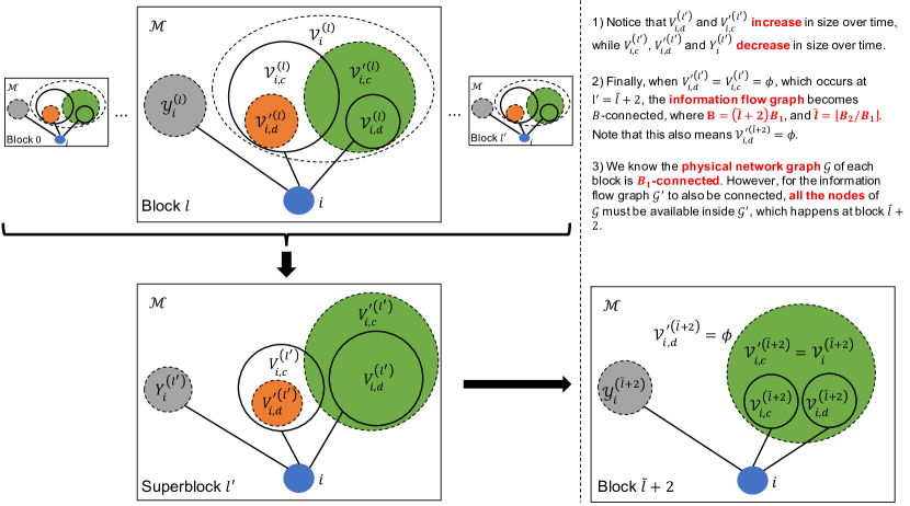
Figure 3: The illustration of definitions and lemmas given for the proof of Proposition 1 in Appendix A.

Definition 2.

We group the set of iterations after an arbitrary iteration $k=0,1,\cdots$ into blocks of $B_{1}$ and we denote block $l$ as iterations $k+lB_{1},\cdots,k+(l+1)B_{1}-1$, for $l=0,1,\cdots$.

Note that under Assumption 8-(a), the graph union of the physical network graph over each of these blocks, that is, $\mathcal{G}^{(k+lB_{1}:k+(l+1)B_{1}-1)}$, is connected for all $k,l\geq 0$. See Fig. 3 for a visualization of blocks.

Definition 3.

At each block $l\geq 0$, device $i\in\mathcal{M}$ is connected to a subset of devices $\mathcal{V}_{i}^{(l)}\in\mathcal{M}$, i.e., the edges $(i,j)$ for $j\in\mathcal{V}_{i}^{(l)}$ are present in $\cup_{s=0}^{B_{1}-1}{\mathcal{E}^{(k+lB_{1}+s)}}$, for all $k\geq 0$. Also, we define $\mathcal{Y}_{i}^{(l)}=\mathcal{M}\setminus\mathcal{V}_{i}^{(l)}\setminus i$ as the devices that are not neighbors of device $i$ at block $l$. In Fig. 3, we illustrate device $i$, $\mathcal{V}_{i}^{(l)}$, $\mathcal{Y}_{i}^{(l)}$ and $\mathcal{M}$ inside each block.

Definition 4.

Given the time-varying network topology, we further split $\mathcal{V}_{i}^{(l)}$ into two disjoint subsets, $\mathcal{V}_{i,c}^{(l)}$ and $\mathcal{V}_{i,d}^{(l)}$, which contain devices connected to and disconnected from device $i$ at the beginning of block $l$, i.e., at iteration $k+lB_{1}$, for all $k,l\geq 0$, respectively.

The devices in $\mathcal{V}_{i,d}^{(l)}$ will eventually become connected to $i\in\mathcal{M}$ during block $l$ due to Assumption 8-(a), for all $l\geq 0$. The subsets $\mathcal{V}_{i,c}^{(l)}$ and $\mathcal{V}_{i,d}^{(l)}$ are illustrated in Fig. 3.

Definition 5.

We divide $\mathcal{V}_{i}^{(l)}$ into two disjoint subsets, $\mathcal{V}^{\prime(l)}_{i,c}$ and $\mathcal{V}^{\prime(l)}_{i,d}$ which, respectively, contain the devices that exchange parameters with device $i\in\mathcal{M}$ and those that do not over the course of the block $l\geq 0$. Note that the edges $(i,j)$ for $j\in\mathcal{V}^{\prime(l)}_{i,c}$ are present in $\cup_{s=0}^{B_{1}-1}{\mathcal{E}^{\prime(k+lB_{1}+s)}}$, for all $k\geq 0$.

To make the subsequent mathematical proofs more clear, we show the subsets $\mathcal{V}^{\prime(l)}_{i,c}$ and $\mathcal{V}^{\prime(l)}_{i,d}$ in Fig. 3. It is important to make the distinction between the four subsets, $\mathcal{V}_{i,c}^{(l)}$ and $\mathcal{V}_{i,d}^{(l)}$ in one hand, $\mathcal{V}^{\prime(l)}_{i,c}$ and $\mathcal{V}^{\prime(l)}_{i,d}$ in the other.

Definition 6.

Starting from any iteration $k\geq 0$, multiple consecutive blocks can be further grouped to form a super block. In our analysis, we focus only on the super block which groups the first blocks $0,\cdots,l^{\prime}$ together for all $l^{\prime}\geq 0$. In other words, the super block consists of iterations $k,\cdots,k+lB_{1},\cdots,k+(l+1)B_{1}-1,\cdots,k+(l^{\prime}+1)B_{1}-1$ where $l$, $0\leq l\leq l^{\prime}$, indicates the $l$-th block and $k\geq 0$.

Definition 7.

For the super block described above, we define the following corresponding sets:

$$\begin{gathered}V_{i}^{(l^{\prime})}=\cup_{l=0}^{l^{\prime}}{\mathcal{V}_{i}^{(l)}},\qquad Y_{i}^{(l^{\prime})}=\cap_{l=0}^{l^{\prime}}{\mathcal{Y}_{i}^{(l)}},\\ V_{i,d}^{(l^{\prime})}=\cup_{l=0}^{l^{\prime}}{\mathcal{V}_{i,d}^{(l)}},\qquad V_{i,c}^{(l^{\prime})}=\cap_{l=0}^{l^{\prime}}{\mathcal{V}_{i,c}^{(l)}},\\ V^{\prime(l^{\prime})}_{i,d}=\cap_{l=0}^{l^{\prime}}{\mathcal{V}^{\prime(l)}_{i,d}},\qquad V^{\prime(l^{\prime})}_{i,c}=\cup_{l=0}^{l^{\prime}}{\mathcal{V}^{\prime(l)}_{i,c}},\end{gathered}$$

for all $i\in\mathcal{M}$ and $l^{\prime}\geq 0$. At the super block $l^{\prime}$, $V_{i}^{(l^{\prime})}$ is the set of all devices that are physically connected to device $i$, and $Y_{i}^{(l^{\prime})}$ contains the devices that do not. Moreover, $V_{i,d}^{(l^{\prime})}$ keeps track of all devices that were initially disconnected from device $i$ at the beginning of each block inside the super block, while $V_{i,c}^{(l^{\prime})}$ only contains those devices that remain connected to device $i$ from the first block up until the last block inside the super block. Similarly, $V^{\prime(l^{\prime})}_{i,d}$ is the set that keeps track of those devices that have not exchanged parameters with device $i$ inside the super block, and $V^{\prime(l^{\prime})}_{i,c}$ contains all the ones that have.

It can be easily shown that $V_{i}^{(l^{\prime})}\cup Y_{i}^{(l^{\prime})}=\mathcal{M}\setminus i$ and $V_{i,d}^{(l^{\prime})}\cup V_{i,c}^{(l^{\prime})}=V^{\prime(l^{\prime})}_{i,d}\cup V^{\prime(l^{\prime})}_{i,c}=V_{i}^{(l^{\prime})}$. Notice that $V_{i,c}^{(l^{\prime})}$ is defined as the intersection of the corresponding subsets in each block, and contains the devices that were connected to the device $i\in\mathcal{M}$ in iteration $k\geq 0$, and stay connected to it at all times until the end of super block at iteration $k+(l^{\prime}+1)B_{1}-1$, for all $l^{\prime}\geq 0$.

Next, we provide two supplementary lemmas which will be useful in proving Proposition 1.

Lemma 7.

The relations that relate the subsets defined in 3, 4, 5 and 7 together are as follows:

1. In each block $l\geq 0$ and for each device $i\in\mathcal{M}$, we have

   $$\mathcal{V}_{i,d}^{(l)}\in\mathcal{V}^{\prime(l)}_{i,c},\qquad\mathcal{V}^{\prime(l)}_{i,d}\in\mathcal{V}_{i,c}^{(l)}.\vspace*{-2mm}$$

2. For super block $l^{\prime}\geq 0$ and each device $i\in\mathcal{M}$, we have

   $$V_{i,d}^{(l^{\prime})}\in V^{\prime(l^{\prime})}_{i,c},\qquad V^{\prime(l^{\prime})}_{i,d}\in V_{i,c}^{(l^{\prime})}.\vspace*{-2mm}$$

3. The set of all devices in $\mathcal{V}_{i,c}^{(l^{\prime}+1)}$ can be partitioned into three disjoint subsets to get a relationship between block $l^{\prime}+1$ and the super block consisting of blocks $0,\cdots,l^{\prime}$, for all $i\in\mathcal{M}$ and $l^{\prime}\geq 0$. We have

   $$\mathcal{V}_{i,c}^{(l^{\prime}+1)}\in V_{i,d}^{(l^{\prime})}\cup V_{i,c}^{(l^{\prime})}\cup\left(Y_{i}^{(l^{\prime})}\cap\mathcal{V}_{i,c}^{(l^{\prime}+1)}\right).\vspace*{-2mm}$$

Proof.

(a) Given Assumption 8-(a), devices in $\mathcal{V}_{i,d}^{(l)}$ will eventually become connected to $i$ in the course of this block. On the other hand, Neighbor Connection Event in Alg. 1 enforces that all of these devices exchange model parameters with device $i$ upon connection. Therefore, the set $\mathcal{V}^{\prime(l)}_{i,c}$ is a super set of $\mathcal{V}_{i,d}^{(l)}$, i.e., $\mathcal{V}_{i,d}^{(l)}\in\mathcal{V}^{\prime(l)}_{i,c}$, and as a result

$$\mathcal{V}^{\prime(l)}_{i,d}=\mathcal{V}_{i}^{(l)}\setminus\mathcal{V}^{\prime(l)}_{i,c}\in\mathcal{V}_{i}^{(l)}\setminus\mathcal{V}^{(l)}_{i,d}=\mathcal{V}^{(l)}_{i,c}.$$

(b) The proof for this follows from Part (a) and the definitions of the sets for the super block. Since $\mathcal{V}_{i,d}^{(l)}\in\mathcal{V}^{\prime(l)}_{i,c}$,

$$V_{i,d}^{(l^{\prime})}=\cup_{l=0}^{l^{\prime}}{\mathcal{V}_{i,d}^{(l)}}\in\cup_{l=0}^{l^{\prime}}{\mathcal{V}^{\prime(l)}_{i,c}}=V^{\prime(l^{\prime})}_{i,c}.$$

On the other hand, since $\mathcal{V}^{\prime(l)}_{i,d}\in\mathcal{V}_{i,c}^{(l)}$, it follows that

$$V^{\prime(l^{\prime})}_{i,d}=\cap_{l=0}^{l^{\prime}}{\mathcal{V}^{\prime(l)}_{i,d}}\in\cap_{l=0}^{l^{\prime}}{\mathcal{V}_{i,c}^{(l)}}=V_{i,c}^{(l^{\prime})}.$$

(c) We show that these three subsets are disjoint. For the first two, take $j\in V_{i,c}^{(l^{\prime})}=\cap_{l=0}^{l^{\prime}}{\mathcal{V}_{i,c}^{(l)}}$, which means $j\in\mathcal{V}_{i,c}^{(l)}$ for all $l=0,\cdots,l^{\prime}$. Hence, we have $j\notin\mathcal{V}_{i}^{(l)}\setminus\mathcal{V}_{i,c}^{(l)}=\mathcal{V}_{i,d}^{(l)}$ for all $l$, so $j\notin\cup_{l=0}^{l^{\prime}}{\mathcal{V}_{i,d}^{(l)}}=V_{i,d}^{(l^{\prime})}$.

For the third set, it can easily be shown that $V_{i,d}^{(l^{\prime})}\cup V_{i,c}^{(l^{\prime})}=V_{i}^{(l^{\prime})}$. We can then prove that $Y_{i}^{(l^{\prime})}$ is disjoint from $V_{i}^{(l^{\prime})}$, since $j\in Y_{i}^{(l^{\prime})}=\cap_{l=0}^{l^{\prime}}{\mathcal{Y}_{i}^{(l)}}$ indicates $j\in\mathcal{Y}_{i}^{(l)}$ for all $l=0,\cdots,l^{\prime}$. Hence, we have $j\notin\mathcal{M}\setminus\mathcal{Y}_{i}^{(l)}\setminus i=\mathcal{V}_{i}^{(l)}$ for all $l$, so $j\notin\cup_{l=0}^{l^{\prime}}{\mathcal{V}_{i}^{(l)}}=V_{i}^{(l^{\prime})}$. $Y_{i}^{(l^{\prime})}$ and $V_{i}^{(l^{\prime})}$ being disjoint implies $Y_{i}^{(l^{\prime})}\cap\mathcal{V}_{i,c}^{(l^{\prime}+1)}$ and $V_{i}^{(l^{\prime})}$ are also disjoint. ∎

Part (a) of the above lemma means that devices initially disconnected from device $i$ which become connected to it over the course of a block will definitely exchange parameters with it upon connection. Therefore, devices that might not exchange parameters with device $i$ inside a block will definitely be among those that were initially connected to it. Part (b) states a similar argument for a super block.

Lemma 8.

The following connectivity characteristics hold for the graph union of the information flow graphs.

1. The union of the information flow graphs within each block $l\geq 0$, from iteration $k+lB_{1}$ to $k+(l+1)B_{1}-1$, that is, $\mathcal{G}^{\prime(k+lB_{1}:k+(l+1)B_{1}-1)}$, is connected only if $\mathcal{V}_{i,c}^{(l)}\in\mathcal{V}^{\prime(l)}_{i,c}$, for all $k\geq 0$.

2. The union of the information flow graphs inside each super block $l^{\prime}\geq 0$, from iteration $k$ to $k+(l^{\prime}+1)B_{1}-1$, that is, $\mathcal{G}^{\prime(k:k+(l^{\prime}+1)B_{1}-1)}$, is connected only if $\mathcal{V}_{i,c}^{(\tilde{l})}\in V^{\prime(l^{\prime})}_{i,c}$ for at least one $\tilde{l}$, $0\leq\tilde{l}\leq l^{\prime}$ and all $k\geq 0$.

Proof.

(a) First, by the definition of each block, running from iteration $k+lB_{1}$ to $k+(l+1)B_{1}-1$ for $l=0,1,\cdots$, the physical network graph $\mathcal{G}^{(k+lB_{1}:k+(l+1)B_{1}-1)}$ is connected. Therefore, if $\mathcal{V}_{i}^{(l)}=\mathcal{V}^{\prime(l)}_{i,c}$, the information flow graph of this block, i.e., $\mathcal{G}^{\prime(k+lB_{1}:k+(l+1)B_{1}-1)}$, will also be connected, since these two graphs are comprised of the same set of edges.

Second, note that $\mathcal{V}^{\prime(l)}_{i,c}\in\mathcal{V}_{i}^{(l)}$ is true by definition, so we only need to show $\mathcal{V}_{i}^{(l)}\in\mathcal{V}^{\prime(l)}_{i,c}$. Since $\mathcal{V}_{i}^{(l)}=\mathcal{V}_{i,d}^{(l)}\cup\mathcal{V}_{i,c}^{(l)}$, and as a consequence of Lemma 7-(a), $\mathcal{V}_{i,d}^{(l)}\in\mathcal{V}^{\prime(l)}_{i,c}$, we must also have the condition $\mathcal{V}_{i,c}^{(l)}\in\mathcal{V}^{\prime(l)}_{i,c}$.

(b) We take steps similar to those in Lemma 8-(a) here. First, it is straightforward to show that connectivity is preserved under graph union. Therefore, if we find a block $\tilde{l}$ inside the super block $l^{\prime}$, $0\leq\tilde{l}\leq l^{\prime}$, such that $\mathcal{V}_{i}^{(\tilde{l})}\in V^{\prime(l^{\prime})}_{i,c}$, then the information flow graph of this super block, i.e., $\mathcal{G}^{\prime(k:k+(l^{\prime}+1)B_{1}-1)}$, will be connected.

Second, by definition, we have $\mathcal{V}_{i}^{(\tilde{l})}=\mathcal{V}_{i,d}^{(\tilde{l})}\cup\mathcal{V}_{i,c}^{(\tilde{l})}$ and $V^{\prime(l^{\prime})}_{i,c}=\cup_{l=0}^{l^{\prime}}{\mathcal{V}^{\prime(l)}_{i,c}}$. Lemma 7-(a) yields $\mathcal{V}_{i,d}^{(\tilde{l})}\in\mathcal{V}^{\prime(\tilde{l})}_{i,c}\in\cup_{l=0}^{l^{\prime}}{\mathcal{V}^{\prime(l)}_{i,c}}$. Thus, we must have $\mathcal{V}_{i,c}^{(\tilde{l})}\in\cup_{l=0}^{l^{\prime}}{\mathcal{V}^{\prime(l)}_{i,c}}=V^{\prime(l^{\prime})}_{i,c}$. ∎

Now we are ready to prove Proposition 1.

Proof.

Lemma 8-(b) states that for the information flow graph $\mathcal{G}^{\prime(k)}$ to be $(l^{\prime}+1)B_{1}$-connected, the relation $\mathcal{V}_{i,c}^{(\tilde{l})}\in V^{\prime(l^{\prime})}_{i,c}$ must hold for at least one $\tilde{l}$, $0\leq\tilde{l}\leq l^{\prime}$. According to Lemma 7-(c), we have $\mathcal{V}_{i,c}^{(\tilde{l}+1)}=V_{i,d}^{(\tilde{l})}\cup V_{i,c}^{(\tilde{l})}\cup(Y_{i}^{(\tilde{l})}\cap\mathcal{V}_{i,c}^{(\tilde{l}+1)})$, therefore we must show $V_{i,d}^{(\tilde{l}-1)}\cup V_{i,c}^{(\tilde{l}-1)}\cup(Y_{i}^{(\tilde{l}-1)}\cap\mathcal{V}_{i,c}^{(\tilde{l})})\in V^{\prime(l^{\prime})}_{i,c}$ to prove connectivity. From Lemma 7-(b),

$$V_{i,d}^{(\tilde{l}-1)}\in V^{\prime(\tilde{l}-1)}_{i,c}\in V^{\prime(\tilde{l}-1)}_{i,c}\cup\left(\cup_{l=\tilde{l}}^{l^{\prime}}{\mathcal{V}^{\prime(l)}_{i,c}}\right)=V^{\prime(l^{\prime})}_{i,c}.$$

$Y_{i}^{(\tilde{l}-1)}\cap\mathcal{V}_{i,c}^{(\tilde{l})}$ describes devices that are connected to $i$ at the beginning of block $\tilde{l}$, i.e., iteration $k+\tilde{l}B_{1}$, but have not been connected to $i$ in any of the previous blocks $0$ to $\tilde{l}-1$, i.e., between iterations $k$ to $k+\tilde{l}B_{1}-1$. Due to Neighbor Connection Event in Alg. 1, these devices exchange parameters with device $i$ upon connection. Thus, $Y_{i}^{(\tilde{l}-1)}\cap\mathcal{V}_{i,c}^{(\tilde{l})}\in\mathcal{V}^{\prime(\tilde{l})}_{i,c}\in V^{\prime(l^{\prime})}_{i,c}$.

Next, we need to prove $V_{i,c}^{(\tilde{l}-1)}\in V^{\prime(l^{\prime})}_{i,c}$. Recall that the set $V_{i,c}^{(\tilde{l}-1)}$ contains devices that have been connected to $i$ from the beginning of block $0$ (iteration $k$) until the beginning of block $\tilde{l}-1$ (iteration $k+(\tilde{l}-1)B_{1}$). Thus, for the devices in this set to exchange parameters with $i$, a Broadcast Event (see Alg. 1) must occur at device $i$. Due to Assumption 8-(b), a Broadcast event is guaranteed at least once every $B_{2}$ iteration on device $i$. If $\tilde{l}B_{1}\leq B_{2}\leq(\tilde{l}+1)B_{1}-1$, we know that a Broadcast event is triggered in the super block $\tilde{l}+1$, causing device $i$ to exchange parameters with its neighboring devices in this super block. As a result, we write $V_{i,c}^{(\tilde{l}+1)}\in\mathcal{V}^{\prime(\tilde{l}+1)}_{i,c}\in V^{\prime(\tilde{l}+1)}_{i,c}$.

Putting everything together concludes the proof, showing that the information flow graph $\mathcal{G}^{\prime(k)}$ is $(l^{\prime}+1)B_{1}$-connected if $l^{\prime}=\tilde{l}+1$, where $\tilde{l}$ is determined by $\tilde{l}B_{1}\leq B_{2}\leq(\tilde{l}+1)B_{1}-1$. Thus, $\mathcal{G}^{\prime(k)}$ is $(\tilde{l}+2)B_{1}$-connected. ∎

Appendix B Proof of Lemma 4

To prove the second inequality, we first bound $\mathbb{E}{[{\|\mathbf{\epsilon}^{(k)}\|}^{2}]}$ as

$$\mathbb{E}{\left[{\left\|\mathbf{\epsilon}^{(k)}\right\|}^{2}\right]}=\mathbb{E}{\left[\sum_{i=1}^{m}{{\left\|\mathbf{\epsilon}_{i}^{(k)}\right\|}^{2}}\right]}=\sum_{i=1}^{m}{\mathbb{E}{\left[{\left\|\mathbf{\epsilon}_{i}^{(k)}\right\|}^{2}\right]}} =\sum_{i=1}^{m}{\sigma_{i}^{2}}$$

$$\leq m\sigma^{2}.$$

Now, we write

$$\mathbb{E} {\left[{\left\|\mathbf{\epsilon}^{(k)}-\mathbf{1}_{m}\mathbf{\bar{\epsilon}}^{(k)}\right\|}^{2}\right]}$$

$$=\mathbb{E}{\left[{\left\|\mathbf{\epsilon}^{(k)}\right\|}^{2}-2\left\langle\mathbf{\epsilon}^{(k)},\mathbf{1}_{m}\mathbf{\bar{\epsilon}}^{(k)}\right\rangle+{\left\|\mathbf{1}_{m}\mathbf{\bar{\epsilon}}^{(k)}\right\|}^{2}\right]}$$

$$=\mathbb{E}{\left[{\left\|\mathbf{\epsilon}^{(k)}\right\|}^{2}\right]}-2\sum_{i=1}^{m}{\mathbb{E}{\left[\left\langle\mathbf{\epsilon}_{i}^{(k)},\mathbf{\bar{\epsilon}}^{(k)}\right\rangle\right]}}+m\mathbb{E}{\left[{\left\|\mathbf{\bar{\epsilon}}^{(k)}\right\|}^{2}\right]}$$

$$\begin{aligned} =\,\,&\mathbb{E}{\left[{\left\|\mathbf{\epsilon}^{(k)}\right\|}^{2}\right]}-\frac{2}{m}\sum_{i=1}^{m}{\mathbb{E}{\left[{\left\|\mathbf{\epsilon}_{i}^{(k)}\right\|}^{2}\right]}}\\ &-\frac{2}{m}\sum_{i=1}^{m}{\left\langle\mathbb{E}{\left[\mathbf{\epsilon}_{i}^{(k)}\right]},\sum_{\begin{subarray}{c}j=1\\ j\neq i\end{subarray}}^{m}{\mathbb{E}{\left[\mathbf{\epsilon}_{j}^{(k)}\right]}}\right\rangle}+m\mathbb{E}{\left[{\left\|\mathbf{\bar{\epsilon}}^{(k)}\right\|}^{2}\right]}\end{aligned}$$

$$\leq m\sigma^{2}+2\sigma^{2}+\sigma^{2}=\left(m+3\right)\sigma^{2}\leq 4m\sigma^{2}.$$

Appendix C Proof of Lemma 5

(a) Note that

$${\left\|\mathbf{\nabla}^{(k)}-\mathbf{1}_{m}\mathbf{\bar{\nabla}}^{(k)}\right\|}^{2} \leq 2{\left\|\mathbf{\nabla}^{(k)}-\nabla{F}^{(k)}\right\|}^{2}$$

$$+2{\left\|\mathbf{1}_{m}\mathbf{\bar{\nabla}}^{(k)}-\nabla{F}^{(k)}\right\|}^{2}.$$

We first bound ${\|\mathbf{\nabla}^{(k)}-\nabla{F}^{(k)}\|}^{2}$ as

$${\left\|\mathbf{\nabla}^{(k)}-\nabla{F}^{(k)}\right\|}^{2} =\sum_{i=1}^{m}{{\left\|\nabla{F_{i}{\left(\mathbf{w}_{i}^{(k)}\right)}}-\nabla{F{\left(\mathbf{w}_{i}^{(k)}\right)}}\right\|}^{2}}$$

$$\leq\sum_{i=1}^{m}{\delta_{i}^{2}}\leq m\delta^{2},$$

in which the data heterogeneity bound $\delta$ of Assumption 5 was used. Next, for ${\|\mathbf{1}_{m}\mathbf{\bar{\nabla}}^{(k)}-\nabla{F}^{(k)}\|}^{2}$, we have

$${\left\|\mathbf{1}_{m}\mathbf{\bar{\nabla}}^{(k)}-\nabla{F}^{(k)}\right\|}^{2}=\sum_{i=1}^{m}{{\left\|\mathbf{\bar{\nabla}}^{(k)}-\nabla{F{\left(\mathbf{w}_{i}^{(k)}\right)}}\right\|}^{2}}$$

$$=\sum_{i=1}^{m}{{\left\|\sum_{j=1}^{m}{\frac{\nabla{F_{j}{\left(\mathbf{w}_{j}^{(k)}\right)}}-\nabla{F_{j}{\left(\mathbf{w}_{i}^{(k)}\right)}}}{m}}\right\|}^{2}}$$

$$\leq\sum_{i=1}^{m}{m\sum_{j=1}^{m}{\frac{{\left\|\nabla{F_{j}{\left(\mathbf{w}_{j}^{(k)}\right)}}-\nabla{F_{j}{\left(\mathbf{w}_{i}^{(k)}\right)}}\right\|}^{2}}{m^{2}}}}$$

$$\leq\sum_{i=1}^{m}{\sum_{j=1}^{m}{\frac{L_{j}^{2}{\left\|\mathbf{w}_{j}^{(k)}-\mathbf{w}_{i}^{(k)}\right\|}^{2}}{m}}}$$

$$\leq L^{2}\sum_{i=1}^{m}{\sum_{j=1}^{m}{\frac{2{\left\|\mathbf{w}_{j}^{(k)}-\mathbf{\bar{w}}^{(k)}\right\|}^{2}+2{\left\|\mathbf{w}_{i}^{(k)}-\mathbf{\bar{w}}^{(k)}\right\|}^{2}}{m}}}$$

$$=4L^{2}\sum_{i=1}^{m}{{\left\|\mathbf{w}_{i}^{(k)}-\mathbf{\bar{w}}^{(k)}\right\|}^{2}}=4L^{2}{\left\|\mathbf{W}^{(k)}-\mathbf{1}_{m}\mathbf{\bar{w}}^{(k)}\right\|}^{2}.$$

where the Lipschitz constant $L$ of Assumption 3 was used. Therefore,

$${\left\|\mathbf{\nabla}^{(k)}-\mathbf{1}_{m}\mathbf{\bar{\nabla}}^{(k)}\right\|}^{2}\leq 2m\delta^{2}+8L^{2}{\left\|\mathbf{W}^{(k)}-\mathbf{1}_{m}\mathbf{\bar{w}}^{(k)}\right\|}^{2}.$$

(b) Next, we bound the difference of the average of local models (13) from the global optimum $\mathbf{w}^{\star}$:

$${\left\|\mathbf{\bar{w}}^{(k+1)}-\mathbf{w}^{\star}\right\|}^{2}={\left\|\mathbf{\bar{w}}^{(k)}-\alpha^{(k)}\mathbf{\bar{g}}^{(k)}-\mathbf{w}^{\star}\right\|}^{2}$$

$$\begin{aligned} =\,\,&{\left\|\mathbf{\bar{w}}^{(k)}-\alpha^{(k)}\mathbf{\bar{\nabla}}^{(k)}-\mathbf{w}^{\star}\right\|}^{2}\\ &-2\alpha^{(k)}\left\langle\mathbf{\bar{w}}^{(k)}-\alpha^{(k)}\mathbf{\bar{\nabla}}^{(k)}-\mathbf{w}^{\star},\mathbf{\bar{\epsilon}}^{(k)}\right\rangle+{\left(\alpha^{(k)}\right)}^{2}{\left\|\mathbf{\bar{\epsilon}}^{(k)}\right\|}^{2}\end{aligned}$$

$$\begin{aligned} \leq\,\,&\left(1+H_{1}^{(k)}\right){\left\|\mathbf{\bar{w}}^{(k)}-\alpha^{(k)}\nabla{F{\left(\mathbf{\bar{w}}^{(k)}\right)}}-\mathbf{w}^{\star}\right\|}^{2}\\ &+\left(1+\frac{1}{H_{1}^{(k)}}\right){\left(\alpha^{(k)}\right)}^{2}{\left\|\nabla{F{\left(\mathbf{\bar{w}}^{(k)}\right)}}-\mathbf{\bar{\nabla}}^{(k)}\right\|}^{2}\\ &-2\alpha^{(k)}\left\langle\mathbf{D^{(k)}},\frac{1}{m}\mathbf{1}_{m}^{\top}\mathbf{\epsilon}^{(k)}\right\rangle+{\left(\alpha^{(k)}\right)}^{2}{\left\|\mathbf{\bar{\epsilon}}^{(k)}\right\|}^{2}\end{aligned}$$

$$\begin{aligned} \leq\,\,&\left(1+H_{1}^{(k)}\right){\left(1-\mu\alpha^{(k)}\right)}^{2}{\left\|\mathbf{\bar{w}}^{(k)}-\mathbf{w}^{\star}\right\|}^{2}\\ &+\left(1+\frac{1}{H_{1}^{(k)}}\right)\frac{{\left(\alpha^{(k)}\right)}^{2}L^{2}}{m}{\left\|\mathbf{W}^{(k)}-\mathbf{1}_{m}\mathbf{\bar{w}}^{(k)}\right\|}^{2}\\ &-2\alpha^{(k)}\left\langle\mathbf{D^{(k)}},\frac{1}{m}\mathbf{1}_{m}^{\top}\mathbf{\epsilon}^{(k)}\right\rangle+{\left(\alpha^{(k)}\right)}^{2}{\left\|\mathbf{\bar{\epsilon}}^{(k)}\right\|}^{2},\end{aligned}$$

where the inequalities of Lemma 3 was used, and $\mathbf{D^{(k)}}\triangleq\mathbf{\bar{w}}^{(k)}-\alpha^{(k)}\mathbf{\bar{\nabla}}^{(k)}-\mathbf{w}^{\star}$. Also note that we can set $H_{1}^{(k)}$ to an arbitrary positive real value. Taking the expected value of this relation and setting $H_{1}^{(k)}=\mu\alpha^{(k)}$, while noting that $\mathbf{D^{(k)}}$ and $\epsilon^{(k)}$ are independent random variables since $\mathbf{\bar{w}}^{(k)}$ only depends on $\mathbf{\epsilon}^{(0)}$ to $\mathbf{\epsilon^{(k-1)}}$, we get

$$\mathbb{E} {\left[{\left\|\mathbf{\bar{w}}^{(k+1)}-\mathbf{w}^{\star}\right\|}^{2}\right]}$$

$$\begin{aligned} \leq\,\,&\left(1-\mu^{2}{\left(\alpha^{(k)}\right)}^{2}\right)\left(1-\mu\alpha^{(k)}\right)\mathbb{E}{\left[{\left\|\mathbf{\bar{w}}^{(k)}-\mathbf{w}^{\star}\right\|}^{2}\right]}\\ &+\left(1+\mu\alpha^{(k)}\right)\frac{\alpha^{(k)}L^{2}}{\mu m}\mathbb{E}{\left[{\left\|\mathbf{W}^{(k)}-\mathbf{1}_{m}\mathbf{\bar{w}}^{(k)}\right\|}^{2}\right]}\\ &+\frac{{\left(\alpha^{(k)}\right)}^{2}\sigma^{2}}{m}\end{aligned}$$

$$\begin{aligned} \leq\,\,&\left(1-\mu\alpha^{(k)}\right)\mathbb{E}{\left[{\left\|\mathbf{\bar{w}}^{(k)}-\mathbf{w}^{\star}\right\|}^{2}\right]}\\ &+\left(1+\mu\alpha^{(k)}\right)\frac{\alpha^{(k)}L^{2}}{\mu m}\mathbb{E}{\left[{\left\|\mathbf{W}^{(k)}-\mathbf{1}_{m}\mathbf{\bar{w}}^{(k)}\right\|}^{2}\right]}\\ &+\frac{{\left(\alpha^{(k)}\right)}^{2}\sigma^{2}}{m},\end{aligned}$$

where the gradient approximation independence of Assumption 6-(c), and the result of Lemma 4 is used. Note that the reason we set $H_{1}^{(k)}=\mu\alpha^{(k)}$ was so that the scalar coefficient of $\mathbb{E}{[{\|\mathbf{\bar{w}}^{(k)}-\mathbf{w}^{\star}\|}^{2}]}$ would become less that $1$, which is essential in our convergence analysis when proving Proposition 2.

(c) Finally, we bound the consensus error of the local learning models to their average value using (10) and (13).

$$\begin{aligned} {\left\|\mathbf{W}^{(k+1)}-\mathbf{1}_{m}\mathbf{\bar{w}}^{(k+1)}\right\|}^{2}&=\Big{\|}\mathbf{P}^{(k)}\mathbf{W}^{(k)}-\mathbf{1}_{m}\mathbf{\bar{w}}^{(k)}\\ &-\alpha^{(k)}\left(\mathbf{G}^{(k)}-\mathbf{1}_{m}\mathbf{\bar{g}}^{(k)}\right)\Big{\|}^{2}\end{aligned}$$ (31)

$$\begin{aligned} =\,\,&{\left\|\mathbf{P}^{(k)}\mathbf{W}^{(k)}-\mathbf{1}_{m}\mathbf{\bar{w}}^{(k)}-\alpha^{(k)}\left(\mathbf{\nabla}^{(k)}-\mathbf{1}_{m}\mathbf{\bar{\nabla}}^{(k)}\right)\right\|}^{2}\\ &\begin{aligned} -2\alpha^{(k)}&\Big{\langle}\mathbf{P}^{(k)}\mathbf{W}^{(k)}-\mathbf{1}_{m}\mathbf{\bar{w}}^{(k)}\\ &-\alpha^{(k)}\left(\mathbf{\nabla}^{(k)}-\mathbf{1}_{m}\mathbf{\bar{\nabla}}^{(k)}\right),\mathbf{\epsilon}^{(k)}-\mathbf{1}_{m}\mathbf{\bar{\epsilon}}^{(k)}\Big{\rangle}\end{aligned}\\ &+{\left(\alpha^{(k)}\right)}^{2}{\left\|\mathbf{\epsilon}^{(k)}-\mathbf{1}_{m}\mathbf{\bar{\epsilon}}^{(k)}\right\|}^{2}\end{aligned}$$

$$\begin{aligned} \leq\,\,&\left(1+H_{2}^{(k)}\right){\left\|\mathbf{P}^{(k)}\mathbf{W}^{(k)}-\mathbf{1}_{m}\mathbf{\bar{w}}^{(k)}\right\|}^{2}\\ &+\left(1+\frac{1}{H_{2}^{(k)}}\right){\left(\alpha^{(k)}\right)}^{2}{\left\|\mathbf{\nabla}^{(k)}-\mathbf{1}_{m}\mathbf{\bar{\nabla}}^{(k)}\right\|}^{2}\\ &-2\alpha^{(k)}\left\langle\mathbf{D^{(k)}},\left(\mathbf{I}-\frac{1}{m}\mathbf{1}_{m}\mathbf{1}_{m}^{\top}\right)\mathbf{\epsilon}^{(k)}\right\rangle\\ &+{\left(\alpha^{(k)}\right)}^{2}{\left\|\mathbf{\epsilon}^{(k)}-\mathbf{1}_{m}\mathbf{\bar{\epsilon}}^{(k)}\right\|}^{2},\end{aligned}$$

where $\mathbf{D}^{(k)}\triangleq\mathbf{P}^{(k)}\mathbf{W}^{(k)}-\mathbf{1}_{m}\mathbf{\bar{w}}^{(k)}-\alpha^{(k)}\left(\mathbf{\nabla}^{(k)}-\mathbf{1}_{m}\mathbf{\bar{\nabla}}^{(k)}\right)$. Now, focusing on the first two terms in the bound, we write

$$\begin{aligned} \left(1+H_{2}^{(k)}\right)&{\left\|\mathbf{P}^{(k)}\mathbf{W}^{(k)}-\mathbf{1}_{m}\mathbf{\bar{w}}^{(k)}\right\|}^{2}\\ &+\left(1+\frac{1}{H_{2}^{(k)}}\right){\left(\alpha^{(k)}\right)}^{2}{\left\|\mathbf{\nabla}^{(k)}-\mathbf{1}_{m}\mathbf{\bar{\nabla}}^{(k)}\right\|}^{2}\end{aligned}$$

$$\begin{aligned} \leq\,\,&\left(1+H_{2}^{(k)}\right){\left(\rho^{(k)}\right)}^{2}{\left\|\mathbf{W}^{(k)}-\mathbf{1}_{m}\mathbf{\bar{w}}^{(k)}\right\|}^{2}\\ &\begin{aligned} +\left(1+\frac{1}{H_{2}^{(k)}}\right){\left(\alpha^{(k)}\right)}^{2}\Bigg{[}&2m\delta^{2}\\ &+8L^{2}{\left\|\mathbf{W}^{(k)}-\mathbf{1}_{m}\mathbf{\bar{w}}^{(k)}\right\|}^{2}\Bigg{]}\end{aligned}\end{aligned}$$

$$\begin{aligned} \leq\Bigg{[}\left(1+H_{2}^{(k)}\right){\left(\rho^{(k)}\right)}^{2}&+8\left(1+\frac{1}{H_{2}^{(k)}}\right){\left(\alpha^{(k)}\right)}^{2}L^{2}\Bigg{]}\\ &{\left\|\mathbf{W}^{(k)}-\mathbf{1}_{m}\mathbf{\bar{w}}^{(k)}\right\|}^{2}\end{aligned}$$

$$+2m\left(1+\frac{1}{H_{2}^{(k)}}\right){\left(\alpha^{(k)}\right)}^{2}\delta^{2},$$

in which the results of Lemma 2 and Part (a) of this lemma were used. Now, putting this inequality back in (31), then taking its expected value with $H_{2}^{(k)}=\frac{2\sqrt{2}\alpha^{(k)}L}{\rho{(k)}}$, noting that $\mathbf{D}^{(k)}$ and $\epsilon^{(k)}$ are independent random variables since $\mathbf{P}^{(k)}\mathbf{W}^{(k)}-\mathbf{1}_{m}\mathbf{\bar{w}}^{(k)}$ only depends on $\mathbf{\epsilon}^{(0)}$ to $\mathbf{\epsilon^{(k-1)}}$, we have

$$\mathbb{E} {\left[{\left\|\mathbf{W}^{(k+1)}-\mathbf{1}_{m}\mathbf{\bar{w}}^{(k+1)}\right\|}^{2}\right]}$$

$$\begin{aligned} \leq\,\,&{\left(\rho^{(k)}+2\sqrt{2}\alpha^{(k)}L\right)}^{2}\mathbb{E}{\left[{\left\|\mathbf{W}^{(k)}-\mathbf{1}_{m}\mathbf{\bar{w}}^{(k)}\right\|}^{2}\right]}\\ &+2m{\left(\alpha^{(k)}\right)}^{2}\left[\frac{\rho^{(k)}+2\sqrt{2}\alpha^{(k)}L}{2\sqrt{2}\alpha^{(k)}L}\delta^{2}+2\sigma^{2}\right],\end{aligned}$$

where the results of Lemma 4 was used. Note that $H_{2}^{(k)}$ was chosen such that $H_{2}^{(k)}=\operatorname*{arg\,min}_{H_{2}^{(k)}}{[(1+H_{2}^{(k)}){(\rho^{(k)})}^{2}+8(1+\frac{1}{H_{2}^{(k)}}){(\alpha^{(k)})}^{2}L^{2}]}$.

Appendix D Proof of Lemma 6

We use (11) and (14) to bound the consensus error of local learning models from their mean value at iteration $k+B$, in which $B$ is the connectivity bound of Proposition 1:

$$\begin{aligned} \Big{\|}&\mathbf{W}^{(k+B)}-\mathbf{1}_{m}\mathbf{\bar{w}}^{(k+B)}\Big{\|}^{2}=\Bigg{\|}\mathbf{P}^{(k+B-1:k)}\mathbf{W}^{(k)}-\mathbf{1}_{m}\mathbf{\bar{w}}^{(k)}\\ &-\sum_{r=k+1}^{k+B-1}{\alpha^{(r-1)}\left(\mathbf{P}^{(k+B-1:r)}\mathbf{G}^{(r-1)}-\mathbf{1}_{m}\mathbf{\bar{g}}^{(r-1)}\right)}\\ &-\alpha^{(k+B-1)}\left(\mathbf{G}^{(k+B-1)}-\mathbf{1}_{m}\mathbf{\bar{g}}^{(k+B-1)}\right)\Bigg{\|}^{2}\end{aligned}$$

$$\begin{aligned} =\Bigg{\|}&\mathbf{P}^{(k+B-1:k)}\mathbf{W}^{(k)}-\mathbf{1}_{m}\mathbf{\bar{w}}^{(k)}\\ &-\sum_{r=k+1}^{k+B}{\alpha^{(r-1)}\left(\mathbf{P}^{(k+B-1:r)}\mathbf{G}^{(r-1)}-\mathbf{1}_{m}\mathbf{\bar{g}}^{(r-1)}\right)}\Bigg{\|}^{2}\end{aligned}$$

$$= \Bigg{\|}\mathbf{P}^{(k+B-1:k)}\mathbf{W}^{(k)}-\mathbf{1}_{m}\mathbf{\bar{w}}^{(k)}$$

$$-\sum_{r=k+1}^{k+B}{\alpha^{(r-1)}\left(\mathbf{P}^{(k+B-1:r)}\mathbf{\nabla}^{(r-1)}-\mathbf{1}_{m}\mathbf{\bar{\nabla}}^{(r-1)}\right)}\Bigg{\|}^{2}$$

$$\begin{aligned} -2&\Bigg{\langle}\mathbf{P}^{(k+B-1:k)}\mathbf{W}^{(k)}-\mathbf{1}_{m}\mathbf{\bar{w}}^{(k)}\\ &-\sum_{r=k+1}^{k+B}{\alpha^{(r-1)}\left(\mathbf{P}^{(k+B-1:r)}\mathbf{\nabla}^{(r-1)}-\mathbf{1}_{m}\mathbf{\bar{\nabla}}^{(r-1)}\right)},\\ &\sum_{r=k+1}^{k+B}{\alpha^{(r-1)}\left(\mathbf{P}^{(k+B-1:r)}\mathbf{\epsilon}^{(r-1)}-\mathbf{1}_{m}\mathbf{\bar{\epsilon}}^{(r-1)}\right)}\Bigg{\rangle}\end{aligned}$$

$$+{\left\|\sum_{r=k+1}^{k+B}{\alpha^{(r-1)}\left(\mathbf{P}^{(k+B-1:r)}\mathbf{\epsilon}^{(r-1)}-\mathbf{1}_{m}\mathbf{\bar{\epsilon}}^{(r-1)}\right)}\right\|}^{2}.$$

Looking only at the inner product term in the above expression, we can write it equivalently as follows

$$-2\left\langle\mathbf{D}^{(k)},\sum_{r=k+1}^{k+B}{\alpha^{(r-1)}\left(\mathbf{P}^{(k+B-1:r)}-\frac{1}{m}\mathbf{1}_{m}\mathbf{1}_{m}^{\top}\right)\mathbf{\epsilon}^{(r-1)}}\right\rangle$$

$$\begin{aligned} +2\Bigg{\langle}&\sum_{r=k+1}^{k+B}{\alpha^{(r-1)}\left(\mathbf{P}^{(k+B-1:r)}\mathbf{\nabla}^{(r-1)}-\mathbf{1}_{m}\mathbf{\bar{\nabla}}^{(r-1)}\right)},\\ &\sum_{r=k+1}^{k+B}{\alpha^{(r-1)}\left(\mathbf{P}^{(k+B-1:r)}-\frac{1}{m}\mathbf{1}_{m}\mathbf{1}_{m}^{\top}\right)\mathbf{\epsilon}^{(r-1)}}\Bigg{\rangle}\leq\end{aligned}$$

$$-2\left\langle\mathbf{D}^{(k)},\sum_{r=k+1}^{k+B}{\alpha^{(r-1)}\left(\mathbf{P}^{(k+B-1:r)}-\frac{1}{m}\mathbf{1}_{m}\mathbf{1}_{m}^{\top}\right)\mathbf{\epsilon}^{(r-1)}}\right\rangle$$

$$+4{\left\|\sum_{r=k+1}^{k+B}{\alpha^{(r-1)}\left(\mathbf{P}^{(k+B-1:r)}\mathbf{\nabla}^{(r-1)}-\mathbf{1}_{m}\mathbf{\bar{\nabla}}^{(r-1)}\right)}\right\|}^{2}$$

$$+4{\left\|\sum_{r=k+1}^{k+B}{\alpha^{(r-1)}\left(\mathbf{P}^{(k+B-1:r)}-\frac{1}{m}\mathbf{1}_{m}\mathbf{1}_{m}^{\top}\right)\mathbf{\epsilon}^{(r-1)}}\right\|}^{2},$$

in which $\mathbf{D}^{(k)}\triangleq\mathbf{P}^{(k+B-1:k)}\mathbf{W}^{(k)}-\mathbf{1}_{m}\mathbf{\bar{w}}^{(k)}$. Going back to ${\left\|\mathbf{W}^{(k+B)}-\mathbf{1}_{m}\mathbf{\bar{w}}^{(k+B)}\right\|}^{2}$, we can bound it as

$$\Big{\|} \mathbf{W}^{(k+B)}-\mathbf{1}_{m}\mathbf{\bar{w}}^{(k+B)}\Big{\|}^{2}$$

$$\leq \left(1+H_{3}\right){\left\|\mathbf{P}^{(k+B-1:k)}\mathbf{W}^{(k)}-\mathbf{1}_{m}\mathbf{\bar{w}}^{(k)}\right\|}^{2}$$

$$\begin{aligned} +\left(5+\frac{1}{H_{3}}\right)B&\sum_{r=k+1}^{k+B}{\left(\alpha^{(r-1)}\right)}^{2}\\ &{\left\|\mathbf{P}^{(k+B-1:r)}\mathbf{\nabla}^{(r-1)}-\mathbf{1}_{m}\mathbf{\bar{\nabla}}^{(r-1)}\right\|}^{2}\end{aligned}$$

$$-2\left\langle\mathbf{D}^{(k)},\sum_{r=k+1}^{k+B}{\alpha^{(r-1)}\left(\mathbf{P}^{(k+B-1:r)}-\frac{1}{m}\mathbf{1}_{m}\mathbf{1}_{m}^{\top}\right)\mathbf{\epsilon}^{(r-1)}}\right\rangle$$

$$+5B\sum_{r=k+1}^{k+B}{{\left(\alpha^{(r-1)}\right)}^{2}{\left\|\mathbf{P}^{(k+B-1:r)}\mathbf{\epsilon}^{(r-1)}-\mathbf{1}_{m}\mathbf{\bar{\epsilon}}^{(r-1)}\right\|}^{2}}$$

$$\leq \left(1+H_{3}\right){\left(\rho^{(k+B-1:k)}\right)}^{2}{\left\|\mathbf{W}^{(k)}-\mathbf{1}_{m}\mathbf{\bar{w}}^{(k)}\right\|}^{2}$$

$$\begin{aligned} +\left(5+\frac{1}{H_{3}}\right)B&\sum_{r=k+1}^{k+B}{\left(\alpha^{(r-1)}\right)}^{2}{\left(\rho^{(k+B-1:r)}\right)}^{2}\\ &{\left\|\mathbf{\nabla}^{(r-1)}-\mathbf{1}_{m}\mathbf{\bar{\nabla}}^{(r-1)}\right\|}^{2}\end{aligned}$$

$$-2\sum_{r=k+1}^{k+B}{\alpha^{(r-1)}\left\langle\mathbf{D}^{(k)},\left(\mathbf{P}^{(k+B-1:r)}-\frac{1}{m}\mathbf{1}_{m}\mathbf{1}_{m}^{\top}\right)\mathbf{\epsilon}^{(r-1)}\right\rangle}$$

$$+5B\sum_{r=k+1}^{k+B}{{\left(\alpha^{(r-1)}\right)}^{2}{\left(\rho^{(k+B-1:r)}\right)}^{2}{\left\|\mathbf{\epsilon}^{(r-1)}-\mathbf{1}_{m}\mathbf{\bar{\epsilon}}^{(r-1)}\right\|}^{2}},$$

in which the results of Lemma 2 is used. Next, we bound $\mathbb{E}{[{\|\mathbf{\nabla}^{(r-1)}-\mathbf{1}_{m}\mathbf{\bar{\nabla}}^{(r-1)}\|}^{2}]}$ using Lemma 5 and using recursion until we reach iteration $k$ in the right-hand side of the inequality as

$$\mathbb{E}{\left[{\left\|\mathbf{\nabla}^{(r-1)}-\mathbf{1}_{m}\mathbf{\bar{\nabla}}^{(r-1)}\right\|}^{2}\right]}$$

$$\leq 2m\delta^{2}+8L^{2}\mathbb{E}{\left[{\left\|\mathbf{W}^{(r-1)}-\mathbf{1}_{m}\mathbf{\bar{w}}^{(r-1)}\right\|}^{2}\right]}$$

$$\begin{aligned} \leq 2&m\delta^{2}+8L^{2}\Bigg{[}a_{21}^{(r-2:k)}\mathbb{E}{\left[{\left\|\mathbf{\bar{w}}^{(k)}-\mathbf{w}^{\star}\right\|}^{2}\right]}\\ &+a_{22}^{(r-2:k)}\mathbb{E}{\left[{\left\|\mathbf{W}^{(k)}-\mathbf{1}_{m}\mathbf{\bar{w}}^{(k)}\right\|}^{2}\right]}\\ &+\sum_{l=k+1}^{r-2}{\left(a_{21}^{(r-2:l)}c_{1}^{(l-1)}+a_{22}^{(r-2:l)}c_{2}^{(l-1)}\right)}+c_{2}^{(r-2)}\Bigg{]}.\end{aligned}$$

Combining the last two sets of inequalities and taking the expected value of ${\|\mathbf{W}^{(k+B)}-\mathbf{1}_{m}\mathbf{\bar{w}}^{(k+B)}\|}^{2}$, with $H_{3}=\frac{1-\rho^{2}}{2\rho^{2}}$ and using the bound $\rho^{(k+B-1:k)}\leq\rho$, it yields

$$\mathbb{E}{\left[{\left\|\mathbf{W}^{(k+B)}-\mathbf{1}_{m}\mathbf{\bar{w}}^{(k+B)}\right\|}^{2}\right]}\leq\Bigg{[}\frac{1+\rho^{2}}{2}$$

$$\begin{aligned} &\begin{aligned} +8&\frac{5-3\rho^{2}}{1-\rho^{2}}BL^{2}\sum_{r=k+1}^{k+B}{\left(\alpha^{(r-1)}\right)}^{2}{\left(\rho^{(k+B-1:r)}\right)}^{2}a_{22}^{(r-2:k)}\Bigg{]}\\ &\mathbb{E}{\left[{\left\|\mathbf{W}^{(k)}-\mathbf{1}_{m}\mathbf{\bar{w}}^{(k)}\right\|}^{2}\right]}\end{aligned}\\ &\begin{aligned} +2&\frac{5-3\rho^{2}}{1-\rho^{2}}B\sum_{r=k+1}^{k+B}{\left(\alpha^{(r-1)}\right)}^{2}{\left(\rho^{(k+B-1:r)}\right)}^{2}\\ &\left(m\delta^{2}+4L^{2}\left[\sum_{l=k+1}^{r-2}{a_{22}^{(r-2:l)}c_{2}^{(l-1)}}+c_{2}^{(r-2)}\right]\right)\end{aligned}\\ &+20mB\sigma^{2}\sum_{r=k+1}^{k+B}{{\left(\alpha^{(r-1)}\right)}^{2}{\left(\rho^{(k+B-1:r)}\right)}^{2}}.\end{aligned}$$

Note that $\mathbf{D}^{(k)}$ and $\epsilon^{(k)}$ are independent random variables, since $\mathbf{P}^{(k+B-1:k)}\mathbf{W}^{(k)}-\mathbf{1}_{m}\mathbf{\bar{w}}^{(k)}$ only depends on $\mathbf{\epsilon}^{(0)}$ to $\mathbf{\epsilon}^{(k-1)}$. . Substituting $\rho^{(k+B-1:r)}<1$ for $k+1\leq r\leq k+B-1$ completes the proof. Note that $H_{3}=\frac{1-\rho^{2}}{2\rho^{2}}$ was chosen such that $(1+H_{3})\rho^{2}<1$ would hold, which is necessary to prove Proposition 2.

Appendix E Proof of Proposition 2

We divide the proof into three steps: (i) obtaining the constraints on the step size, (ii) obtaining some bounds for the matrix entries of (26), and (iii) providing the final results.

(i) We obtain the conditions under which $\rho{(\mathbf{\Phi}^{(k)})}<1$. We have $\rho{(\mathbf{\Phi}^{(k)})}=\max{\{\lambda_{1}^{(k)},\lambda_{2}^{(k)}\}}$, where $\lambda_{1}^{(k)}$ and $\lambda_{2}^{(k)}$ are eigenvalues of $\mathbf{\Phi}^{(k)}$. Since $\phi_{21}^{(k)}=0$ (see (25)), we have

$$\det{\left(\lambda\mathbf{I}-\mathbf{\Phi}^{(k)}\right)}=\left(\lambda-\phi_{11}^{(k)}\right)\left(\lambda-\phi_{22}^{(k)}\right).$$

Consequently, we need $\phi_{11}^{(k)},\phi_{22}^{(k)}<1$. If $\alpha^{(0)}<\frac{2}{\mu+L}$, which implies $\alpha^{(k)}<\frac{2}{\mu+L}$, we have from (25), (23) and (21) that

$$\begin{gathered}\phi_{11}^{(k)}=a_{11}^{(\left(k+1\right)B-1:kB)}=\prod_{r=kB}^{\left(k+1\right)B-1}{\left(1-\mu\alpha^{(r)}\right)}<1\\ \Rightarrow\quad\alpha^{(0)}<\frac{1}{\mu},\end{gathered}$$

which trivially holds since $\mu<L$, and thus $\alpha^{(0)}<\frac{2}{\mu+L}<\frac{2}{2\mu}=\frac{1}{\mu}$. Next, for $\phi_{22}^{(k)}\leq\frac{3+\rho^{2}}{4}<1$, we must have:

$$\phi_{22}^{(k)}=\frac{1+\rho^{2}}{2}+8\frac{5-3\rho^{2}}{1-\rho^{2}}BL^{2}\sum_{r=kB+1}^{\left(k+1\right)B}{\left(\alpha^{(r-1)}\right)}^{2}a_{22}^{(r-2:k)}$$

$$\begin{aligned} \Rightarrow\sum_{r=kB+1}^{\left(k+1\right)B}{\left(\alpha^{(r-1)}\right)}^{2}&\prod_{l=kB}^{r-2}{{\left(1+2\sqrt{2}\alpha^{(l)}L\right)}^{2}}\\ &\leq\frac{{\left(1-\rho^{2}\right)}^{2}}{32\left(5-3\rho^{2}\right)BL^{2}},\end{aligned}$$

in which (23) and (21) were used. Next, to further analyze the above inequality, we introduce an extra constraint on the non-increasing step size, such that $\alpha^{(k)}\leq\frac{\Gamma}{2\sqrt{2}L}$ where $\Gamma>0$ can be any positive real value. Now we have

$$\sum_{r=kB+1}^{\left(k+1\right)B}{\left(\alpha^{(r-1)}\right)}^{2}\prod_{l=kB}^{r-2}{{\left(1+2\sqrt{2}\alpha^{(l)}L\right)}^{2}}$$

$$\leq\sum_{r=kB+1}^{\left(k+1\right)B}{\left(\alpha^{(r-1)}\right)}^{2}\prod_{l=kB}^{r-2}{{\left(1+\Gamma\right)}^{2}}$$

$$\leq\sum_{r=kB+1}^{\left(k+1\right)B}{\left(\alpha^{(r-1)}\right)}^{2}{\left(1+\Gamma\right)}^{2\left(r-1-kB\right)}$$

$$\leq B{\left(\alpha^{(kB)}\right)}^{2}{\left(1+\Gamma\right)}^{2\left(B-1\right)}.$$

As a result, we can obtain the second constraint on the upper bound for the step size as

$$B{\left(\alpha^{(kB)}\right)}^{2}{\left(1+\Gamma\right)}^{2\left(B-1\right)}\leq\frac{{\left(1-\rho^{2}\right)}^{2}}{32\left(5-3\rho^{2}\right)BL^{2}},$$

$$\Rightarrow\alpha^{(0)}\leq\frac{1-\rho^{2}}{4\sqrt{2}\sqrt{5-3\rho^{2}}BL{\left(1+\Gamma\right)}^{B-1}}.$$

Thus, we can finally conclude the constraint

$$\alpha^{(0)}\leq\min{\left\{\frac{\Gamma}{2\sqrt{2}L},\frac{1-\rho^{2}}{4\sqrt{2}\sqrt{5-3\rho^{2}}BL{\left(1+\Gamma\right)}^{B-1}}\right\}}.$$

Note that $\Gamma>0$, and increasing it from $0$ to $\infty$ will increase the first constraint from $0$ to $\infty$, while decreasing the second one from $\frac{1-\rho^{2}}{4\sqrt{2}\sqrt{5-3\rho^{2}}BL}$ to $0$. Thus, we find the optimal value of $\Gamma$ next. We can say that there is a crossing point $\Gamma_{0}>0$ such that

$$\begin{cases}\frac{\Gamma}{2\sqrt{2}L}\leq\frac{1-\rho^{2}}{4\sqrt{2}\sqrt{5-3\rho^{2}}BL{\left(1+\Gamma\right)}^{B-1}}&0<\Gamma\leq\Gamma_{0}\\ \frac{1-\rho^{2}}{4\sqrt{2}\sqrt{5-3\rho^{2}}BL{\left(1+\Gamma\right)}^{B-1}}\leq\frac{\Gamma}{2\sqrt{2}L}&\Gamma\geq\Gamma_{0}\end{cases}.$$

So, by introducing an auxiliary function $H{(\cdot)}$ as follows,

$$H{\left(x\right)}=x{\left(1+x\right)}^{B-1}-\frac{1-\rho^{2}}{2\sqrt{5-3\rho^{2}}B},$$

we will have $H{\left(\Gamma_{0}\right)}=0$.

However, we are not interested in calculating the exact value of $\Gamma_{0}$, but instead we obtain the following bounds for it

$$H{\left(0\right)}=-\frac{1-\rho^{2}}{2\sqrt{5-3\rho^{2}}B}<0,$$

$$\begin{aligned} H{\left(\frac{1-\rho^{2}}{2\sqrt{5-3\rho^{2}}B}\right)}=\frac{1-\rho^{2}}{2\sqrt{5-3\rho^{2}}B}\Bigg{[}&{\left(1+\frac{1-\rho^{2}}{2\sqrt{5-3\rho^{2}}B}\right)}^{B-1}\\ &-1\Bigg{]}\geq 0,\end{aligned}$$

$$\Rightarrow\Gamma_{0}\in\Bigg{(}0,\frac{1-\rho^{2}}{2\sqrt{5-3\rho^{2}}B}\Bigg{]}.$$

Note that we have $\Gamma_{1}=\frac{1-\rho^{2}}{2\sqrt{5-3\rho^{2}}B}\leq\frac{1}{2\sqrt{2}B}\leq\frac{1}{2\sqrt{2}}$, and $\Gamma_{1}\geq\Gamma_{0}$. Thus, setting $\Gamma=\Gamma_{1}$ will yield the following constraint

$$\alpha^{(0)}\leq\frac{1-\rho^{2}}{4\sqrt{2}\sqrt{5-3\rho^{2}}BL{\left(1+\Gamma_{1}\right)}^{B-1}}.$$

In order to build an intuition to understand this bound, we can substitute the upper-bound of $\Gamma_{1}$ to get the following

$$\frac{1-\rho^{2}}{4\sqrt{10}BL{\left(1+\frac{1}{2\sqrt{2}}\right)}^{B-1}}\leq\frac{1-\rho^{2}}{4\sqrt{2}\sqrt{5-3\rho^{2}}BL{\left(1+\Gamma_{1}\right)}^{B-1}}$$

$$\leq\frac{\Gamma_{1}}{2\sqrt{2}L}=\frac{\Gamma_{1}}{2\sqrt{2}}\frac{2}{2L}\leq\frac{1}{8}\frac{2}{\mu+L}\leq\frac{2}{\mu+L}.$$

(ii) Next, we derive the following bounds for (21):

$$a_{22}^{(k)}\leq{\left(1+\Gamma\right)}^{2},$$

$$c_{2}^{(k)}=2m{\left(\alpha^{(k)}\right)}^{2}\left(\frac{1+\Gamma}{2\sqrt{2}\alpha^{(k)}L}\delta^{2}+2\sigma^{2}\right).$$

Second, for (25):

$$\phi_{11}^{(k)}\geq{\left(1-\mu\alpha^{(kB+1)}\right)}^{B},$$

$$\phi_{22}^{(k)}\leq\frac{1+\rho^{2}}{2}+8\frac{5-3\rho^{2}}{1-\rho^{2}}B^{2}L^{2}{\left(\alpha^{(kB)}\right)}^{2}{\left(1+\Gamma\right)}^{2\left(B-1\right)}.$$

Similarly for (23):

$$a_{12}^{(k+B-1:k)}=a_{11}^{(k+B-1)}a_{12}^{(k+B-2:k)}+a_{12}^{(k+B-1)}a_{22}^{(k+B-2:k)}$$

$$=a_{11}^{(k+B-1:k+1)}a_{12}^{(k)}+\sum_{r=k+2}^{k+B}{a_{11}^{(k+B-1:r)}a_{12}^{(r-1)}a_{22}^{(r-2:k)}}$$

$$=\sum_{r=k+1}^{k+B}{a_{11}^{(k+B-1:r)}a_{12}^{(r-1)}a_{22}^{(r-2:k)}}$$

$$\begin{aligned} \leq\sum_{r=k+1}^{k+B}{\left(a_{11}^{(k+B-1)}\right)}^{k+B-r}&a_{12}^{(r-1)}\left(a_{22}^{(r-2)}\right)^{r-1-k}\end{aligned}$$

$$\leq Ba_{12}^{(k)}{\left(a_{22}^{(k)}\right)}^{B-1}\leq B\left(1+\mu\alpha^{(k)}\right)\frac{\alpha^{(k)}L^{2}}{\mu m}{\left(1+\Gamma\right)}^{2\left(B-1\right)}.$$

Finally, we find an upper-bound for  (26). We have from part (i) that $0<\phi_{11}^{(k)},\phi_{22}^{(k)}<1$. Next, we obtain bounds for $\psi_{1}^{(k)}$ and $\psi_{2}^{(k)}$, but note that we only need them to be bounded constants

$$\begin{aligned} \psi_{1}^{(k)}\leq\,\,&{\left(\alpha^{(kB)}\right)}^{2}\Bigg{\{}\left(B-1\right)\Bigg{[}\left(1-\mu\alpha^{(\left(k+1\right)B-1)}\right)\frac{\sigma^{2}}{m}\\ &\begin{aligned} +2&\left(B-1\right)\left(1+\mu\alpha^{(kB+1)}\right)\frac{\alpha^{(kB+1)}L^{2}}{\mu}\\ &{\left(1+\Gamma\right)}^{2\left(B-2\right)}\left(\frac{1+\Gamma}{2\sqrt{2}\alpha^{(kB)}L}\delta^{2}+2\sigma^{2}\right)\Bigg{]}+\frac{\sigma^{2}}{m}\Bigg{\}}\end{aligned}\end{aligned}$$

$$\leq{\left(\alpha^{(kB)}\right)}^{2}B\left\{\frac{\sigma^{2}}{m}+\nu^{(kB)}\right\},$$

$$\begin{aligned} \psi_{2}^{(k)}=2&B^{2}{\left(\alpha^{(kB)}\right)}^{2}\Bigg{\{}\frac{5-3\rho^{2}}{1-\rho^{2}}\Bigg{[}m\delta^{2}\\ &\begin{aligned} +8mL^{2}&{\left(\alpha^{(k)}\right)}^{2}\left(\frac{1+\Gamma}{2\sqrt{2}\alpha^{(k)}L}\delta^{2}+2\sigma^{2}\right)\\ &\left(B-1\right){\left(1+\Gamma\right)}^{2\left(B-2\right)}\Bigg{]}+10m\sigma^{2}\Bigg{\}}\end{aligned}\end{aligned}$$

$$\leq 10m{\left(\alpha^{(kB)}\right)}^{2}B^{2}\left\{\frac{\delta^{2}+2\mu\alpha^{(kB)}\nu^{(kB)}}{1-\rho^{2}}+2\sigma^{2}\right\},$$

where we have defined

$$\nu^{(k)}=\frac{4}{\mu}\left(B-1\right)L^{2}{\left(1+\Gamma\right)}^{2\left(B-1\right)}\left(\frac{1+\Gamma}{2\sqrt{2}L}\delta^{2}+2\alpha^{(k)}\sigma^{2}\right).$$

(iii) It can be seen that as $k$ goes from $0$ to $\infty$, $\phi_{11}^{(k)}$ increases from ${(1-\mu\alpha^{(1)})}^{B}$ to $1$, and $\phi_{22}^{(k)}$ decreases from $\frac{1+\rho^{2}}{2}+8\frac{5-3\rho^{2}}{1-\rho^{2}}B^{2}L^{2}{(\alpha^{(0)})}^{2}{(1+\Gamma)}^{2(B-1)}$ to $\frac{1+\rho^{2}}{2}$. Therefore, since $\frac{1+\rho^{2}}{2}<1$, there is an iteration $K\geq 0$ where the inequality $\phi_{11}^{(K)}\geq\phi_{22}^{(K)}$ holds for the first time, i.e., $\phi_{11}^{(k)}\leq\phi_{22}^{(k)}$ for all $0\leq k<K$. Consequently, we have

$$\rho{\left(\mathbf{\Phi}^{(k)}\right)}=\begin{cases}\phi_{22}^{(k)}&0\leq k<K\\ \phi_{11}^{(k)}&k\geq K\end{cases}.$$

Note that $K=0$ is also possible, which happens if ${(1-\mu\alpha^{(1)})}^{B}\geq\frac{1+\rho^{2}}{2}+8\frac{5-3\rho^{2}}{1-\rho^{2}}B^{2}L^{2}{(\alpha^{(0)})}^{2}{(1+\Gamma)}^{2(B-1)}$. As a result, we write

$$\begin{aligned} &\begin{bmatrix}\mathbb{E}{\left[{\left\|\mathbf{\bar{w}}^{(kB)}-\mathbf{w}^{\star}\right\|}^{2}\right]}\\ \mathbb{E}{\left[{\left\|\mathbf{W}^{(kB)}-\mathbf{1}_{m}\mathbf{\bar{w}}^{(kB)}\right\|}^{2}\right]}\end{bmatrix}\\ \leq\,\,&\mathbf{\Phi}^{(k-1:K)}\mathbf{\Phi}^{(K-1:0)}\begin{bmatrix}\mathbb{E}{\left[{\left\|\mathbf{\bar{w}}^{(0)}-\mathbf{w}^{\star}\right\|}^{2}\right]}\\ \mathbb{E}{\left[{\left\|\mathbf{W}^{(0)}-\mathbf{1}_{m}\mathbf{\bar{w}}^{(0)}\right\|}^{2}\right]}\end{bmatrix}\\ &+\sum_{r=1}^{k-1}{\mathbf{\Phi}^{(k-1:K)}\mathbf{\Phi}^{(K-1:r)}\mathbf{\Psi}^{(r-1)}}+\mathbf{\Psi}^{(k-1)}\end{aligned}$$

$$\begin{aligned} \leq\,\,&\mathcal{O}{\left(\phi_{11}^{(k-1:K)}\right)}\mathcal{O}{\left(\phi_{22}^{(K-1:0)}\right)}\begin{bmatrix}\mathbb{E}{\left[{\left\|\mathbf{\bar{w}}^{(0)}-\mathbf{w}^{\star}\right\|}^{2}\right]}\\ \mathbb{E}{\left[{\left\|\mathbf{W}^{(0)}-\mathbf{1}_{m}\mathbf{\bar{w}}^{(0)}\right\|}^{2}\right]}\end{bmatrix}\\ &+\mathcal{O}{\left(\phi_{11}^{(k-1:K)}\right)}\sum_{r=1}^{K-1}{\mathcal{O}{\left(\phi_{22}^{(K-1:r)}\right)}\mathbf{\Psi}^{(r-1)}}\\ &+\sum_{r=K}^{k-1}{\mathcal{O}{\left(\phi_{11}^{(k-1:r)}\right)}\mathbf{\Psi}^{(r-1)}}+\mathbf{\Psi}^{(k-1)}.\end{aligned}$$

Appendix F Proof of Theorem 1

If a constant step size $\alpha>0$ is used, i.e., $\alpha^{(k)}=\alpha$ for all $k\geq 0$, the values in (21), (23), (25), (26) and (28) will be time-invariant. Therefore, the inequalities in (27) become

$$\begin{bmatrix}\mathbb{E}{\left[{\left\|\mathbf{\bar{w}}^{(\left(k+1\right)B)}-\mathbf{w}^{\star}\right\|}^{2}\right]}\\ \mathbb{E}{\left[{\left\|\mathbf{W}^{(\left(k+1\right)B)}-\mathbf{1}_{m}\mathbf{\bar{w}}^{(\left(k+1\right)B)}\right\|}^{2}\right]}\end{bmatrix}$$ (32)

$$\leq\mathbf{\Phi}^{k-s+1}\begin{bmatrix}\mathbb{E}{\left[{\left\|\mathbf{\bar{w}}^{(s)}-\mathbf{w}^{\star}\right\|}^{2}\right]}\\ \mathbb{E}{\left[{\left\|\mathbf{W}^{(s)}-\mathbf{1}_{m}\mathbf{\bar{w}}^{(s)}\right\|}^{2}\right]}\end{bmatrix}$$

$$+\left(\sum_{r=s+1}^{k}{\mathbf{\Phi}^{k-r+1}}+1\right)\mathbf{\Psi}.$$

Therefore, (30) in the results of Proposition 2 imply that the following condition must hold to have $\rho{(\mathbf{\Phi})}<1$:

$$\alpha\leq\frac{1-\rho^{2}}{4\sqrt{2}\sqrt{5-3\rho^{2}}BL{\left(1+\Gamma_{1}\right)}^{B-1}}.$$

Finally, we employ (30) to obtain the bounds for $\psi_{1}$ and $\psi_{2}$ as:

$$\begin{gathered}\psi_{1}\leq\alpha^{2}B\left\{\frac{\sigma^{2}}{m}+\nu\right\},\\ \psi_{2}\leq 10m\alpha^{2}B^{2}\left\{\frac{\delta^{2}+2\mu\alpha\nu}{1-\rho^{2}}+2\sigma^{2}\right\},\\ \nu=\frac{4}{\mu}\left(B-1\right)L^{2}{\left(1+\Gamma\right)}^{2\left(B-1\right)}\left(\frac{1+\Gamma}{2\sqrt{2}L}\delta^{2}+2\alpha\sigma^{2}\right).\end{gathered}$$ (33)

Appendix G Proof of Lemma 1

We start by reciprocating the left-hand side of the inequality we want to prove. We have

$$\frac{1}{\prod_{r=s}^{k}{{\left(1-\zeta_{r}\right)}^{p}}}=\prod_{r=s}^{k}{\frac{1}{{\left(1-\zeta_{r}\right)}^{p}}}=\prod_{r=s}^{k}{{\left(1-\zeta_{r}\right)}^{-p}}$$

$$\geq\prod_{r=s}^{k}{\left(1+p\zeta_{r}\right)}=H{\left(k,s\right)},$$

in which Bernoulli’s inequality was used and we defined $H{(k,s)}$ as the lower bound for the reciprocate. Next, we claim that $H{(k,s)}\geq 1+p\sum_{r=s}^{k}{\zeta_{r}}$ for $k\geq s$, and prove it using induction. We have

$$H{\left(s,s\right)}=1+p\zeta_{s}\geq 1+p\zeta_{s},$$

$$H{\left(k+1,s\right)}=\left(1+p\zeta_{k+1}\right)H{\left(k,s\right)}$$

$$\geq\left(1+p\zeta_{k+1}\right)\left(1+p\sum_{r=s}^{k}{\zeta_{r}}\right)$$

$$=1+p\sum_{r=s}^{k+1}{\zeta_{r}}+p^{2}\zeta_{k+1}\sum_{r=s}^{k}{\zeta_{r}}\geq 1+p\sum_{r=s}^{k+1}{\zeta_{r}}.$$

As a result, we get

$$\frac{1}{\prod_{r=s}^{k}{{\left(1-\zeta_{r}\right)}^{p}}}\geq 1+p\sum_{r=s}^{k}{\zeta_{r}}\geq p\sum_{r=s}^{k}{\zeta_{r}}.$$

Finally, the statement of this lemma is proved by taking the reciprocal of the last line above.

Appendix H Proof of Theorem 2

Noting that $\phi_{11}^{(k:s)}$ and $\phi_{22}^{(k:s)}$ are used in the results of Proposition 2, first we derive bounds for these quantities separately using relations (28), (25), (23) and (21) as follows:

$$\phi_{11}^{(k:s)} =\prod_{r=sB}^{\left(k+1\right)B-1}{\left(1-\mu\alpha^{(r)}\right)}\leq\frac{1}{\mu\sum_{r=sB}^{\left(k+1\right)B-1}{\alpha^{(r)}}},$$ (34)

$$\phi_{22}^{(k:s)} \leq\prod_{r=s}^{k}{\frac{3+\rho^{2}}{4}}={\left(\frac{3+\rho^{2}}{4}\right)}^{k-s+1},$$

where Lemma 1 was used to prove the first line, and by satisfying the constraint that $\alpha^{(0)}\leq\frac{1-\rho^{2}}{4\sqrt{2}\sqrt{5-3\rho^{2}}BL{(1+\Gamma_{1})}^{B-1}}$ where $\Gamma_{1}=\frac{1-\rho^{2}}{2\sqrt{5-3\rho^{2}}B}$, the results of Appendix E were used to prove the second line.

The bound in Proposition 2 consists of four terms: (i) $\mathcal{O}{(\phi_{11}^{(k-1:K)})}\mathcal{O}{(\phi_{22}^{(K-1:0)})}$ and (ii) $\mathcal{O}{(\phi_{11}^{(k-1:K)})}\sum_{r=1}^{K-1}{\mathcal{O}{(\phi_{22}^{(K-1:r)})}\Psi^{(r-1)}}$, both of which are the product of a constant and a diminishing term, and thus will converge to $0$ as $k\to\infty$; (iii) $\sum_{r=K}^{k-1}{\mathcal{O}{(\phi_{11}^{(k-1:r)})}\mathbf{\Psi}^{(r-1)}}$ which is the product of an increasing and a decreasing term, and (iv) $\mathbf{\Psi}^{(k-1)}$ which diminishes over time. Terms (i) and (ii) can be easily determined by using the values of (34), and (iv) is obtained via (30), but bounding (iii) needs one extra step as follows

$$\sum_{r=K}^{k-1}{\phi_{11}^{(k-1:r)}\mathbf{\Psi}^{(r-1)}}\leq$$ (35)

$$\sum_{r=K}^{k-1}{\frac{{\left(\alpha^{(\left(r-1\right)B)}\right)}^{2}B}{\mu\sum_{l=rB}^{kB-1}{\alpha^{(l)}}}\begin{bmatrix}\left\{\frac{\sigma^{2}}{m}+\nu^{(0)}\right\}\\ 10mB\left\{\frac{\delta^{2}+2\mu\alpha^{(0)}\nu^{(0)}}{1-\rho^{2}}+2\sigma^{2}\right\}\end{bmatrix}},$$

where we have defined

$$\nu^{(k)}=\frac{4}{\mu}\left(B-1\right)L^{2}{\left(1+\Gamma_{1}\right)}^{2\left(B-1\right)}\left(\frac{1+\Gamma_{1}}{2\sqrt{2}L}\delta^{2}+2\alpha^{(k)}\sigma^{2}\right).$$

Noting the summations in (34) and (35), we first provide the following supplementary lemma for their values, substituting the diminishing step size with the specific choice of $\alpha^{(k)}=\frac{\alpha^{(0)}}{{(1+\nicefrac{{k}}{{\gamma}})}^{\theta}}$ with $\theta=0.5$.

Lemma 9.

If the diminishing step size is chosen as $\alpha^{(k)}=\frac{\alpha^{(0)}}{\sqrt{1+\nicefrac{{k}}{{\gamma}}}}$, the following inequalities hold

1. $$\sum_{r=sB}^{\left(k+1\right)B-1}{\alpha^{(r)}}\geq 2\alpha^{(0)}\left(\sqrt{1+\frac{k+1}{\nicefrac{{\gamma}}{{B}}}}-\sqrt{1+\frac{s}{\nicefrac{{\gamma}}{{B}}}}\right).$$

2. $$\sum_{r=s}^{k}{\frac{{\left(\alpha^{(\left(r-1\right)B)}\right)}^{2}}{\sum_{l=rB}^{\left(k+1\right)B-1}{\alpha^{(l)}}}}\leq\frac{\frac{\alpha^{(0)}}{2}\left(1+\frac{1}{\nicefrac{{\gamma}}{{B}}}\right)}{\sqrt{1+\frac{k+1}{\nicefrac{{\gamma}}{{B}}}}-\sqrt{1+\frac{s}{\nicefrac{{\gamma}}{{B}}}}}$$

   $$+\frac{\alpha^{(0)}\left(1+\nicefrac{{\gamma}}{{B}}\right)}{\sqrt{1+\frac{k+1}{\nicefrac{{\gamma}}{{B}}}}}\left[\ln{\sqrt{1+\frac{k+1}{\nicefrac{{\gamma}}{{B}}}}}+\ln{\frac{1}{\sqrt{1+\frac{1}{\nicefrac{{\gamma}}{{B}}+k}}-1}}\right].$$

Proof.

(a) We can find a lower-bound for the summation by changing it to an integral as

$$\sum_{r=sB}^{\left(k+1\right)B-1}{\alpha^{(r)}} \geq\int_{sB}^{\left(k+1\right)B}{\alpha^{(x)}\,dx}$$

$$=\int_{sB}^{\left(k+1\right)B}{\frac{\alpha^{(0)}}{\sqrt{1+\nicefrac{{x}}{{\gamma}}}}\,dx}$$

$$=2\alpha^{(0)}\left(\sqrt{1+\frac{k+1}{\nicefrac{{\gamma}}{{B}}}}-\sqrt{1+\frac{s}{\nicefrac{{\gamma}}{{B}}}}\right).$$

(b) Similarly, we can find an upper-bound for the summation by changing it to an integral. But first we substitute the bound obtained in Part (a) of this lemma to get

$$\sum_{r=s}^{k}{\frac{{\left(\alpha^{(\left(r-1\right)B)}\right)}^{2}}{\sum_{l=rB}^{\left(k+1\right)B-1}{\alpha^{(l)}}}}$$

$$\leq\sum_{r=s}^{k}{\frac{\alpha^{(0)}}{2\left(1+\frac{r-1}{\nicefrac{{\gamma}}{{B}}}\right)\left(\sqrt{1+\frac{k+1}{\nicefrac{{\gamma}}{{B}}}}-\sqrt{1+\frac{r}{\nicefrac{{\gamma}}{{B}}}}\right)}}$$

$$\leq\sum_{r=s}^{k}{\frac{\frac{\alpha^{(0)}}{2}\left(1+\frac{1}{\nicefrac{{\gamma}}{{B}}}\right)}{\left(1+\frac{r}{\nicefrac{{\gamma}}{{B}}}\right)\left(\sqrt{1+\frac{k+1}{\nicefrac{{\gamma}}{{B}}}}-\sqrt{1+\frac{r}{\nicefrac{{\gamma}}{{B}}}}\right)}}$$

$$\leq\frac{\frac{\alpha^{(0)}}{2}\left(1+\frac{1}{\nicefrac{{\gamma}}{{B}}}\right)}{\left(1+\frac{s}{\nicefrac{{\gamma}}{{B}}}\right)\left(\sqrt{1+\frac{k+1}{\nicefrac{{\gamma}}{{B}}}}-\sqrt{1+\frac{s}{\nicefrac{{\gamma}}{{B}}}}\right)}$$

$$+\int_{s}^{k}{\frac{\frac{\alpha^{(0)}}{2}\left(1+\frac{1}{\nicefrac{{\gamma}}{{B}}}\right)\,dx}{\left(1+\frac{x}{\nicefrac{{\gamma}}{{B}}}\right)\left(\sqrt{1+\frac{k+1}{\nicefrac{{\gamma}}{{B}}}}-\sqrt{1+\frac{x}{\nicefrac{{\gamma}}{{B}}}}\right)}}.$$

Focusing only on the integral term in the above expression without its constant coefficient, and changing the variable to $u{(x)}=\sqrt{1+\frac{x}{\nicefrac{{\gamma}}{{B}}}}$, the integral becomes equal to

$$\int_{s}^{k}{\frac{2\left(\nicefrac{{\gamma}}{{B}}\right)\,d{u{\left(x\right)}}}{u{\left(x\right)}\left[u{\left(k+1\right)}-u{\left(x\right)}\right]}}$$

$$=\frac{2\left(\nicefrac{{\gamma}}{{B}}\right)}{u{\left(k+1\right)}}\left[\int_{s}^{k}{\frac{d{u{\left(x\right)}}}{u{\left(x\right)}}}+\int_{s}^{k}{\frac{d{u{\left(x\right)}}}{u{\left(k+1\right)}-u{\left(x\right)}}}\right]$$

$$=\frac{2\left(\nicefrac{{\gamma}}{{B}}\right)}{u{\left(k+1\right)}}\left[\ln{\frac{u{\left(k\right)}}{u{\left(s\right)}}}+\ln{\frac{u{\left(k+1\right)}-u{\left(s\right)}}{u{\left(k+1\right)}-u{\left(k\right)}}}\right]$$

$$\leq\frac{2\left(\nicefrac{{\gamma}}{{B}}\right)}{u{\left(k+1\right)}}\ln{\frac{u{\left(k\right)}u{\left(k+1\right)}}{u{\left(k+1\right)}-u{\left(k\right)}}}$$

$$\leq\frac{2\left(\nicefrac{{\gamma}}{{B}}\right)}{u{\left(k+1\right)}}\left[\ln{u{\left(k+1\right)}}+\ln{\frac{1}{\frac{u{\left(k+1\right)}}{u{\left(k\right)}}-1}}\right]$$

$$\leq\frac{2\left(\nicefrac{{\gamma}}{{B}}\right)}{\sqrt{1+\frac{k+1}{\nicefrac{{\gamma}}{{B}}}}}\left[\ln{\sqrt{1+\frac{k+1}{\nicefrac{{\gamma}}{{B}}}}}+\ln{\frac{1}{\sqrt{1+\frac{1}{\nicefrac{{\gamma}}{{B}}+k}}-1}}\right].$$

Putting all the terms together proves the statement of the lemma. ∎

Finally, we substitute the results of Lemma 9 and the bounds of (34) accordingly in Proposition 2, to conclude the proof of Theorem 2. We have

$$\begin{aligned} &\begin{bmatrix}\mathbb{E}{\left[{\left\|\mathbf{\bar{w}}^{(kB)}-\mathbf{w}^{\star}\right\|}^{2}\right]}\\ \mathbb{E}{\left[{\left\|\mathbf{W}^{(kB)}-\mathbf{1}_{m}\mathbf{\bar{w}}^{(kB)}\right\|}^{2}\right]}\end{bmatrix}\\ &\begin{aligned} \leq\,\,&\mathcal{O}{\left(\phi_{11}^{(k-1:K)}\right)}\mathcal{O}{\left(\phi_{22}^{(K-1:0)}\right)}\begin{bmatrix}\mathbb{E}{\left[{\left\|\mathbf{\bar{w}}^{(0)}-\mathbf{w}^{\star}\right\|}^{2}\right]}\\ \mathbb{E}{\left[{\left\|\mathbf{W}^{(0)}-\mathbf{1}_{m}\mathbf{\bar{w}}^{(0)}\right\|}^{2}\right]}\end{bmatrix}\end{aligned}\\ &+\mathcal{O}{\left(\phi_{11}^{(k-1:K)}\right)}\sum_{r=1}^{K-1}{\mathcal{O}{\left(\phi_{22}^{(K-1:r)}\right)}\mathbf{\Psi}^{(r-1)}}\\ &+\sum_{r=K}^{k-1}{\mathcal{O}{\left(\phi_{11}^{(k-1:r)}\right)}\mathbf{\Psi}^{(r-1)}}+\mathbf{\Psi}^{(k-1)}\end{aligned}$$ (36)

$$\begin{aligned} &\leq\frac{1}{2\mu\alpha^{(0)}}\mathcal{O}{\left(\frac{1}{\sqrt{k}}\right)}{\left(\frac{3+\rho^{2}}{4}\right)}^{K}\begin{bmatrix}\mathbb{E}{\left[{\left\|\mathbf{\bar{w}}^{(0)}-\mathbf{w}^{\star}\right\|}^{2}\right]}\\ \mathbb{E}{\left[{\left\|\mathbf{W}^{(0)}-\mathbf{1}_{m}\mathbf{\bar{w}}^{(0)}\right\|}^{2}\right]}\end{bmatrix}\\ &\begin{aligned} +\Bigg{\{}&\frac{1}{2\mu\alpha^{(0)}}\mathcal{O}{\left(\frac{1}{\sqrt{k}}\right)}\left(K-1\right)\left(\frac{1+\rho^{2}}{2}\right)\\ &+\frac{\alpha^{(0)}}{2}\mathcal{O}{\left(\frac{\ln{k}}{\sqrt{k}}\right)}+{(\alpha^{(0)})}^{2}\mathcal{O}{\left(\frac{1}{k}\right)}\Bigg{\}}B\begin{bmatrix}\widehat{\psi}_{1}\\ \widehat{\psi}_{2}\end{bmatrix},\end{aligned}\end{aligned}$$

where

$$\begin{gathered}\widehat{\psi}_{1}=\frac{\sigma^{2}}{m}+\nu^{(0)},\qquad\widehat{\psi}_{2}=10mB\left\{\frac{\delta^{2}+2\mu\alpha^{(0)}\nu^{(0)}}{1-\rho^{2}}+2\sigma^{2}\right\},\\ \nu^{(k)}=\frac{4}{\mu}\left(B-1\right)L^{2}{\left(1+\Gamma_{1}\right)}^{2\left(B-1\right)}\left(\frac{1+\Gamma_{1}}{2\sqrt{2}L}\delta^{2}+2\alpha^{(k)}\sigma^{2}\right).\end{gathered}$$

Note that $\ln{\frac{1}{\sqrt{1+\frac{1}{\nicefrac{{\gamma}}{{B}}+k}}-1}}\leq\mathcal{O}{\left(\ln{k}\right)}$.

Appendix I Convergence Results for the General Diminishing Step Size Policy

We mentioned in Assumption 7-(b) that choosing a decreasing step size policy in the form of $\alpha^{(k)}=\frac{\alpha^{(0)}}{{(1+\nicefrac{{k}}{{\gamma}})}^{\theta}}$ satisfies that assumption for $\theta\in(0.5,1]$. We then provided the convergence results for the case of setting $\theta=0.5$ in Theorem 2, which gives us a $\frac{\ln{k}}{\sqrt{k}}$ convergence rate. In this appendix, we touch on similar convergence results for all values of $\theta$.

We first provide a lemma similar to Lemma 9, but for all values of $\theta$. The main difference in the following lemma is that the lower-bound of and the upper-bound of Lemma 9-(a) and 9-(b), respectively, will be different.

Lemma 10.

If the diminishing step size is chosen as $\alpha^{(k)}=\frac{\alpha^{(0)}}{{(1+\nicefrac{{k}}{{\gamma}})}^{\theta}}$ with $\theta=\frac{Q}{Q+1}$ for all integers $Q\geq 2$, the following inequalities hold

1. $$\sum_{r=sB}^{\left(k+1\right)B-1}{\alpha^{(r)}}\geq\frac{\alpha^{(0)}}{1-\theta}\Bigg{(} {\left(1+\frac{k+1}{\nicefrac{{\gamma}}{{B}}}\right)}^{1-\theta}$$

   $$-{\left(1+\frac{s}{\nicefrac{{\gamma}}{{B}}}\right)}^{1-\theta}\Bigg{)},$$

2. $$\sum_{r=s}^{k}{\frac{{\left(\alpha^{(\left(r-1\right)B)}\right)}^{2}}{\sum_{l=rB}^{\left(k+1\right)B-1}{\alpha^{(l)}}}}\leq\frac{{\left(1+\frac{1}{\nicefrac{{\gamma}}{{B}}}\right)}^{2\theta}\alpha^{(0)}\left(1-\theta\right)}{{\left(1+\frac{k+1}{\nicefrac{{\gamma}}{{B}}}\right)}^{1-\theta}-{\left(1+\frac{s}{\nicefrac{{\gamma}}{{B}}}\right)}^{1-\theta}}$$

   $$+\frac{\alpha^{(0)}\left(\nicefrac{{\gamma}}{{B}}\right){\left(1+\frac{1}{\nicefrac{{\gamma}}{{B}}}\right)}^{2\theta}}{{\left(1+\frac{k+1}{\nicefrac{{\gamma}}{{B}}}\right)}^{\theta}}\Bigg{[}\ln{{\left(1+\frac{k+1}{\nicefrac{{\gamma}}{{B}}}\right)}^{1-\theta}}$$

   $$-\ln{\frac{1}{{\left(1+\frac{1}{\nicefrac{{\gamma}}{{B}}+k}\right)}^{1-\theta}-1}}\Bigg{]}$$

   $$+\sum_{q=2}^{Q}{\frac{\alpha^{(0)}\left(\nicefrac{{\gamma}}{{B}}\right){\left(1+\frac{1}{\nicefrac{{\gamma}}{{B}}}\right)}^{2\theta}}{q-1}\frac{1}{{\left(1+\frac{k+1}{\nicefrac{{\gamma}}{{B}}}\right)}^{1-\frac{q}{Q+1}}}}.$$

Proof.

(a) The proof is similar to the proof of Lemma 9-(a), replacing general $\theta$, where $0.5<\theta<1$.

(b) The proof is similar to the proof of Lemma 9-(b), replacing general $\theta$, where $0.5<\theta<1$. The major difference here is the integral part $\int_{s}^{k}{\frac{\left(1-\theta\right)\alpha^{(0)}\,dx}{{\left(1+\frac{x}{\nicefrac{{\gamma}}{{B}}}\right)}^{2\theta}\left({\left(1+\frac{k+1}{\nicefrac{{\gamma}}{{B}}}\right)}^{1-\theta}-{\left(1+\frac{x}{\nicefrac{{\gamma}}{{B}}}\right)}^{1-\theta}\right)}}$, as we will elaborate next. Using a change of variable as $u{(x)}={(1+\frac{x}{\nicefrac{{\gamma}}{{B}}})}^{1-\theta}={(1+\frac{x}{\nicefrac{{\gamma}}{{B}}})}^{\frac{1}{Q+1}}$, the integral (not including its constant coefficients) becomes equal to

$$\int_{s}^{k}{\frac{\frac{\nicefrac{{\gamma}}{{B}}}{1-\theta}\,d{u{\left(x\right)}}}{{u{\left(x\right)}}^{Q}\left[u{\left(k+1\right)}-u{\left(x\right)}\right]}}$$

$$=\frac{\nicefrac{{\gamma}}{{B}}}{1-\theta}\int_{s}^{k}{\left[\sum_{q=1}^{Q}{\frac{\frac{1}{u{\left(k+1\right)}^{Q+1-q}}}{u{\left(x\right)}^{q}}}+\frac{\frac{1}{u{\left(k+1\right)}^{Q}}}{u{\left(k+1\right)}-u{\left(x\right)}}\right]\,d{u{\left(x\right)}}}$$

$$\begin{aligned} =\frac{\nicefrac{{\gamma}}{{B}}}{1-\theta}\Bigg{[}\frac{\ln{\left(\frac{u{\left(k\right)}}{u{\left(s\right)}}\right)}}{u{\left(k+1\right)}^{Q}}&+\sum_{q=2}^{Q}{\frac{\frac{1}{u{\left(s\right)}^{q-1}}-\frac{1}{u{\left(k\right)}^{q-1}}}{\left(q-1\right)u{\left(k+1\right)}^{Q+1-q}}}\\ &+\frac{\ln{\left(\frac{u{\left(k+1\right)}-u{\left(s\right)}}{u{\left(k+1\right)}-u{\left(k\right)}}\right)}}{u{\left(k+1\right)}^{Q}}\Bigg{]}\end{aligned}$$

$$\leq\frac{\nicefrac{{\gamma}}{{B}}}{1-\theta}\left[\frac{\ln{\left(\frac{u{\left(k\right)}u{\left(k+1\right)}}{u{\left(k+1\right)}-u{\left(k\right)}}\right)}}{u{\left(k+1\right)}^{Q}}+\sum_{q=2}^{Q}{\frac{1}{\left(q-1\right)u{\left(k+1\right)}^{Q+1-q}}}\right]$$

$$\begin{aligned} =\frac{\frac{\nicefrac{{\gamma}}{{B}}}{1-\theta}}{u{\left(k+1\right)}^{Q}}&\left[\ln{u{\left(k+1\right)}}+\ln{\frac{1}{\frac{u{\left(k+1\right)}}{u{\left(k\right)}}-1}}\right]\\ &+\sum_{q=2}^{Q}{\frac{\frac{\nicefrac{{\gamma}}{{B}}}{1-\theta}}{q-1}\frac{1}{u{\left(k+1\right)}^{Q+1-q}}}.\end{aligned}$$

∎

Note that although we started this appendix trying to prove the results for any real value of $\theta\in(0.5,1]$, where $\theta$ is constant inside the step size policy of $\alpha^{(k)}=\frac{\alpha^{(0)}}{{\left(1+\frac{k}{\nicefrac{{\gamma}}{{B}}}\right)}^{\theta}}$, in Lemma 10 we were able to derive an upper bound in part (b) only for the choices of $\theta=\frac{Q}{Q+1}$, where $Q\geq 1$ is an integer .

Next, we provide another supplementary lemma for the case $\theta=1$.

Lemma 11.

If the diminishing step size is chosen as $\alpha^{(k)}=\frac{\alpha^{(0)}}{1+\nicefrac{{k}}{{\gamma}}}$, the following inequalities hold

1. $$\sum_{r=sB}^{\left(k+1\right)B-1}{\alpha^{(r)}}\geq\alpha^{(0)}\ln{\left(\frac{1+\frac{k+1}{\nicefrac{{\gamma}}{{B}}}}{1+\frac{s}{\nicefrac{{\gamma}}{{B}}}}\right)},$$

2. $$\sum_{r=s}^{k}{\frac{{\left(\alpha^{(\left(r-1\right)B)}\right)}^{2}}{\sum_{l=rB}^{\left(k+1\right)B-1}{\alpha^{(l)}}}}\leq\frac{{\left(1+\frac{1}{\nicefrac{{\gamma}}{{B}}}\right)}^{2}\alpha^{(0)}}{\ln{\left(\frac{1+\frac{k+1}{\nicefrac{{\gamma}}{{B}}}}{1+\frac{s}{\nicefrac{{\gamma}}{{B}}}}\right)}}$$

   $$\begin{aligned} +\frac{\alpha^{(0)}\left(1+\nicefrac{{\gamma}}{{B}}\right)\left(1+\frac{1}{\nicefrac{{\gamma}}{{B}}}\right)}{1+\frac{k+1}{\nicefrac{{\gamma}}{{B}}}}\Bigg{[}&\operatorname*{li}{\left(1+\frac{k+1}{\nicefrac{{\gamma}}{{B}}}\right)}\\ &+\left\lvert\operatorname*{li}{\left(1+\frac{1}{\nicefrac{{\gamma}}{{B}}+k}\right)}\right\rvert\Bigg{]}.\end{aligned}$$

Proof.

(a) The proof is similar to the proof of Lemma 9-(a), replacing $\theta=1$.

(b) The proof is similar to the proof of Lemma 9-(b), replacing $\theta=1$. The major difference here is the integral part $\int_{s}^{k}{\frac{\alpha^{(0)}\,dx}{{\left(1+\frac{x}{\nicefrac{{\gamma}}{{B}}}\right)}^{2}\ln{\left(\frac{1+\frac{k+1}{\nicefrac{{\gamma}}{{B}}}}{1+\frac{s}{\nicefrac{{\gamma}}{{B}}}}\right)}}}$, as we will elaborate next. Using a change of variable as $u{(x)}=\frac{1+\frac{k+1}{\nicefrac{{\gamma}}{{B}}}}{1+\frac{x}{\nicefrac{{\gamma}}{{B}}}}$, the integral (not including its constant coefficients) becomes equal to

$$\int_{s}^{k}{\frac{\frac{-\nicefrac{{\gamma}}{{B}}}{1+\frac{k+1}{\nicefrac{{\gamma}}{{B}}}}\,d{u{\left(x\right)}}}{\ln{\left(u{\left(x\right)}\right)}}}=\frac{\nicefrac{{\gamma}}{{B}}}{1+\frac{k+1}{\nicefrac{{\gamma}}{{B}}}}\left[\operatorname*{li}{\left(u{\left(s\right)}\right)}-\operatorname*{li}{\left(u{\left(k\right)}\right)}\right]$$

$$\leq\frac{\nicefrac{{\gamma}}{{B}}}{1+\frac{k+1}{\nicefrac{{\gamma}}{{B}}}}\left[\operatorname*{li}{\left(u{\left(s\right)}\right)}+\left\lvert\operatorname*{li}{\left(u{\left(k\right)}\right)}\right\rvert\right],$$

in which $\operatorname*{li}{(x)}=\int_{0}^{x}{\frac{dt}{\ln{(t)}}}$ is the logarithmic integral function. ∎

In order to obtain an expression for the upper-bound in Lemma 11-(b) which is easier to understand, we look at the properties of the logarithmic integral function. We have

$$\begin{cases}\operatorname*{li}(x)\leq 0&x\in[0,1)\cup(1,\mu]\\ \operatorname*{li}(x)\geq 0&x\geq\mu\end{cases},$$

in which $\mu\approx 1.45$ is the zero-crossing point of $\operatorname*{li}(x)$, and is known as the Ramanujan-Soldner constant. Furthermore, the asymptotic behavior of this function is as follows

$$\lim_{x\to\infty}{\frac{\operatorname*{li}(x)}{\frac{x}{\ln{(x)}}}}=1,\qquad\lim_{x\to 1^{+}}{\frac{\operatorname*{li}(x)}{\ln{(x-1)}}}=1.$$

Therefore,

$$\operatorname*{li}{\left(1+\frac{k+1}{\nicefrac{{\gamma}}{{B}}}\right)}+\left\lvert\operatorname*{li}{\left(1+\frac{1}{\nicefrac{{\gamma}}{{B}}+k}\right)}\right\rvert$$

$$\leq\mathcal{O}{\left(\frac{k}{\ln{k}}\right)}+\mathcal{O}{\left(\ln{k}\right)}\leq\mathcal{O}{\left(\frac{k}{\ln{k}}\right)}.$$

Ultimately, by combining Lemma 10 and Lemma 11, we conclude that utilizing a diminishing step size policy $\alpha^{(k)}=\frac{\alpha^{(0)}}{{\left(1+\nicefrac{{k}}{{\gamma}}\right)}^{\theta}}$ with a general $\theta\in(0.5,1]$ changes the results of Theorem 2 in the following manner

$$\begin{bmatrix}\mathbb{E}{\left[{\left\|\mathbf{\bar{w}}^{(kB)}-\mathbf{w}^{\star}\right\|}^{2}\right]}\\ \mathbb{E}{\left[{\left\|\mathbf{W}^{(kB)}-\mathbf{1}_{m}\mathbf{\bar{w}}^{(kB)}\right\|}^{2}\right]}\end{bmatrix}\leq\begin{cases}\mathcal{O}{\left(\frac{\ln{k}}{\sqrt{k}}\right)}&\theta=0.5\\ \mathcal{O}{\left(\frac{1}{k^{1-\theta}}\right)}&0.5<\theta<1\\ \mathcal{O}{\left(\frac{1}{\ln{k}}\right)}&\theta=1\end{cases}.$$

Appendix J Experiments with a Non-Convex Model

We use the same simulation setup used in Sec. IV-A, and we employ the LeNet5 convolutional neural network model, which does not satisfy the convexity assumption (see 4). The loss function $\ell_{\xi}{(\mathbf{w})}$ in (1) is chosen as the cross-entropy loss for LeNet5.

A network of $m=10$ devices is used in simulations and the evaluation is performed only using the Fashion-MNIST data set. The commmunication topology is generated as a random geometric graph with connectivity $0.4$ [11], and to generate non-i.i.d. data distributions across devices, each device only contains samples of the data set from a subset of labels, specifically $2$ labels/device in these experiments. Note that in Fig. 4(iv), we change the simulation setup and set $r=b_{M}\times 10^{-3}$, and let the devices have samples of only $1$ labels/device.

Looking at Fig. 4, we can see that results similar to those of the SVM classifier (see Fig. 2 and Sec. IV-B) can be achieved with the LeNet5 classifier as well, i.e., the results hold with and without the model convexity assumption used in our convergence analysis.

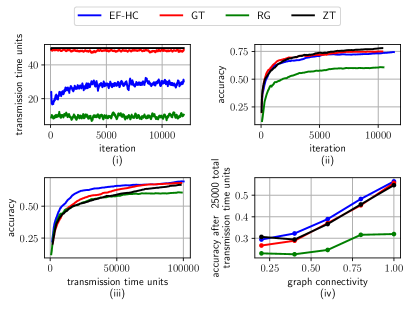
Figure 4: LeNet5 classifier on Fashion-MNIST data set.

References

- [1] S. Zehtabi, S. Hosseinalipour, and C. G. Brinton, “Decentralized event-triggered federated learning with heterogeneous communication thresholds,” IEEE Conf. Decision Control, 2022.
- [2] P. Kairouz, H. B. McMahan, B. Avent, A. Bellet, M. Bennis, A. N. Bhagoji, K. Bonawitz, Z. Charles, G. Cormode, R. Cummings et al., “Advances and open problems in federated learning,” Found. Trends® ML, vol. 14, no. 1–2, pp. 1–210, 2021.
- [3] J. Konečnỳ, H. B. McMahan, F. X. Yu, P. Richtárik, A. T. Suresh, and D. Bacon, “Federated learning: Strategies for improving communication efficiency,” arXiv preprint arXiv:1610.05492, 2016.
- [4] S. Niknam, H. S. Dhillon, and J. H. Reed, “Federated learning for wireless communications: Motivation, opportunities, and challenges,” IEEE Communications Magazine, vol. 58, no. 6, pp. 46–51, 2020.
- [5] S. Wang, Y. Ruan, Y. Tu, S. Wagle, C. G. Brinton, and C. Joe-Wong, “Network-aware optimization of distributed learning for fog computing,” IEEE/ACM Transactions on Networking, vol. 29, no. 5, pp. 2019–2032, 2021.
- [6] M. Chiang and T. Zhang, “Fog and IoT: An overview of research opportunities,” IEEE IoT J., vol. 3, no. 6, pp. 854–864, 2016.
- [7] S. Wang, T. Tuor, T. Salonidis, K. K. Leung, C. Makaya, T. He, and K. Chan, “Adaptive federated learning in resource constrained edge computing systems,” IEEE J. Sel. Areas in Commun., vol. 37, no. 6, pp. 1205–1221, 2019.
- [8] K. Bonawitz, H. Eichner, W. Grieskamp, D. Huba, A. Ingerman, V. Ivanov, C. Kiddon, J. Konečnỳ, S. Mazzocchi, B. McMahan et al., “Towards federated learning at scale: System design,” Proc. Machine Learn. Sys., vol. 1, pp. 374–388, 2019.
- [9] T. Li, A. K. Sahu, A. Talwalkar, and V. Smith, “Federated learning: Challenges, methods, and future directions,” IEEE Signal Proc. Mag., vol. 37, no. 3, pp. 50–60, 2020.
- [10] S. Hosseinalipour, C. G. Brinton, V. Aggarwal, H. Dai, and M. Chiang, “From federated to fog learning: Distributed machine learning over heterogeneous wireless networks,” IEEE Commun. Mag., vol. 58, no. 12, pp. 41–47, 2020.
- [11] S. Hosseinalipour, S. S. Azam, C. G. Brinton, N. Michelusi, V. Aggarwal, D. J. Love, and H. Dai, “Multi-stage hybrid federated learning over large-scale D2D-enabled fog networks,” IEEE/ACM Trans. Network., 2022.
- [12] J. Tsitsiklis, D. Bertsekas, and M. Athans, “Distributed asynchronous deterministic and stochastic gradient optimization algorithms,” IEEE Trans. Auto. Control, vol. 31, no. 9, pp. 803–812, 1986.
- [13] A. Nedic and A. Ozdaglar, “Distributed subgradient methods for multi-agent optimization,” IEEE Trans. Auto. Control, vol. 54, no. 1, pp. 48–61, 2009.
- [14] A. Nedic, A. Ozdaglar, and P. A. Parrilo, “Constrained consensus and optimization in multi-agent networks,” IEEE Trans. Auto. Control, vol. 55, no. 4, pp. 922–938, 2010.
- [15] S. Pu and A. Nedić, “Distributed stochastic gradient tracking methods,” Math. Program., vol. 187, no. 1, pp. 409–457, 2021.
- [16] A. Nedić and A. Olshevsky, “Distributed optimization over time-varying directed graphs,” IEEE Trans. Auto. Control, vol. 60, no. 3, pp. 601–615, 2014.
- [17] R. Xin and U. A. Khan, “A linear algorithm for optimization over directed graphs with geometric convergence,” IEEE Control Sys. Lett., vol. 2, no. 3, pp. 315–320, 2018.
- [18] S. Boyd, P. Diaconis, and L. Xiao, “Fastest mixing markov chain on a graph,” SIAM review, vol. 46, no. 4, pp. 667–689, 2004.
- [19] L. Xiao and S. Boyd, “Fast linear iterations for distributed averaging,” Sys. & Control Lett., vol. 53, no. 1, pp. 65–78, 2004.
- [20] B. Gharesifard and J. Cortés, “When does a digraph admit a doubly stochastic adjacency matrix?” in Proc. American Control Conf. (ACC), 2010, pp. 2440–2445.
- [21] F. Saadatniaki, R. Xin, and U. A. Khan, “Decentralized optimization over time-varying directed graphs with row and column-stochastic matrices,” IEEE Transactions on Automatic Control, vol. 65, no. 11, pp. 4769–4780, 2020.
- [22] S. Pu, W. Shi, J. Xu, and A. Nedić, “Push–pull gradient methods for distributed optimization in networks,” IEEE Trans. Auto. Control, vol. 66, no. 1, pp. 1–16, 2020.
- [23] M. S. Assran and M. G. Rabbat, “Asynchronous gradient push,” IEEE Trans. on Auto. Control, vol. 66, no. 1, pp. 168–183, 2020.
- [24] N. Bof, R. Carli, G. Notarstefano, L. Schenato, and D. Varagnolo, “Multiagent newton–raphson optimization over lossy networks,” IEEE Trans. Auto. Control, vol. 64, no. 7, pp. 2983–2990, 2018.
- [25] H. Wang, Z. Kaplan, D. Niu, and B. Li, “Optimizing federated learning on non-iid data with reinforcement learning,” in IEEE INFOCOM 2020-IEEE Conference on Computer Communications. IEEE, 2020, pp. 1698–1707.
- [26] T. Nishio and R. Yonetani, “Client selection for federated learning with heterogeneous resources in mobile edge,” in IEEE Int. Conf. Commun. (ICC), 2019, pp. 1–7.
- [27] H. T. Nguyen, V. Sehwag, S. Hosseinalipour, C. G. Brinton, M. Chiang, and H. V. Poor, “Fast-convergent federated learning,” IEEE J. Sel. Areas Commun., vol. 39, no. 1, pp. 201–218, 2020.
- [28] E. Diao, J. Ding, and V. Tarokh, “Heterofl: Computation and communication efficient federated learning for heterogeneous clients,” in Int. Conf. Learn. Represent. (ICLR), 2020.
- [29] X. Gu, K. Huang, J. Zhang, and L. Huang, “Fast federated learning in the presence of arbitrary device unavailability,” Advances Neur. Info. Process. Sys. (NeurIPS), vol. 34, 2021.
- [30] N. Shlezinger, M. Chen, Y. C. Eldar, H. V. Poor, and S. Cui, “Federated learning with quantization constraints,” in ICASSP 2020-2020 IEEE International Conference on Acoustics, Speech and Signal Processing (ICASSP). IEEE, 2020, pp. 8851–8855.
- [31] C. Renggli, S. Ashkboos, M. Aghagolzadeh, D. Alistarh, and T. Hoefler, “Sparcml: High-performance sparse communication for machine learning,” in Proceedings of the International Conference for High Performance Computing, Networking, Storage and Analysis, 2019, pp. 1–15.
- [32] S. Savazzi, M. Nicoli, and V. Rampa, “Federated learning with cooperating devices: A consensus approach for massive IoT networks,” IEEE Internet Things J., vol. 7, no. 5, pp. 4641–4654, 2020.
- [33] A. Lalitha, O. C. Kilinc, T. Javidi, and F. Koushanfar, “Peer-to-peer federated learning on graphs,” arXiv preprint arXiv:1901.11173, 2019.
- [34] F. P.-C. Lin, S. Hosseinalipour, S. S. Azam, C. G. Brinton, and N. Michelusi, “Semi-decentralized federated learning with cooperative D2D local model aggregations,” IEEE J. Sel. Areas Commun., vol. 39, no. 12, pp. 3851–3869, 2021.
- [35] J. George and P. Gurram, “Distributed stochastic gradient descent with event-triggered communication,” in Proc. AAAI Conf. Artif. Intell., vol. 34, 2020, pp. 7169–7178.
- [36] S. Sundhar Ram, A. Nedić, and V. V. Veeravalli, “Distributed stochastic subgradient projection algorithms for convex optimization,” J. Optim. Theory App., vol. 147, no. 3, pp. 516–545, 2010.
- [37] S. Pu, A. Olshevsky, and I. C. Paschalidis, “A sharp estimate on the transient time of distributed stochastic gradient descent,” IEEE Trans. Auto. Control, 2021.
- [38] G. Qu and N. Li, “Harnessing smoothness to accelerate distributed optimization,” IEEE Trans. Control Network Sys., vol. 5, no. 3, pp. 1245–1260, 2017.
- [39] H. Xiao, K. Rasul, and R. Vollgraf, “Fashion-mnist: a novel image dataset for benchmarking machine learning algorithms,” arXiv preprint arXiv:1708.07747, 2017.
- [40] S. Caldas, S. M. K. Duddu, P. Wu, T. Li, J. Konečnỳ, H. B. McMahan, V. Smith, and A. Talwalkar, “Leaf: A benchmark for federated settings,” arXiv preprint arXiv:1812.01097, 2018.