(Nearly) Model-Independent Constraints on the Neutral Hydrogen Fraction in the Intergalactic Medium at $z\sim 5-7$ Using Dark Pixel Fractions in Ly$\alpha$ and Ly$\beta$ Forests

Abstract

Cosmic reionization was the last major phase transition of hydrogen from neutral to highly ionized in the intergalactic medium (IGM). Current observations show that the IGM is significantly neutral at $z>7$, and largely ionized by $z\sim 5.5$. However, most methods to measure the IGM neutral fraction are highly model-dependent, and are limited to when the volume-averaged neutral fraction of the IGM is either relatively low ($\overline{x}_{\rm HI}\lesssim 10^{-3}$) or close to unity ($\overline{x}_{\rm HI}\sim 1$). In particular, the neutral fraction evolution of the IGM at the critical redshift range of $z=6-7$ is poorly constrained. We present new constraints on $\overline{x}_{\rm HI}$ at $z\sim 5.1-6.8$, by analyzing deep optical spectra of $53$ quasars at $5.73<z<7.09$. We derive model-independent upper limits on the neutral hydrogen fraction based on the fraction of “dark” pixels identified in the Lyman $\alpha$ (Ly$\alpha$) and Lyman $\beta$ (Ly$\beta$) forests, without any assumptions on the IGM model or the intrinsic shape of the quasar continuum. They are the first model-independent constraints on the IGM neutral hydrogen fraction at $z\sim 6.2-6.8$ using quasar absorption measurements. Our results give upper limits of $\overline{x}_{\rm HI}(z=6.3)<0.79\pm 0.04$ (1$\sigma$), $\overline{x}_{\rm HI}(z=6.5)<0.87\pm 0.03$ (1$\sigma$), and $\overline{x}_{\rm HI}(z=6.7)<0.94^{+0.06}_{-0.09}$ (1$\sigma$). The dark pixel fractions at $z>6.1$ are consistent with the redshift evolution of the neutral fraction of the IGM derived from the Planck 2018.

1 Introduction

Cosmic reionization was the epoch that started when UV photons from the first luminous sources ionized neutral hydrogen in the intergalactic medium (IGM) and ended the dark ages. Reionization was the last major phase transition of hydrogen in the IGM, influencing almost every baryon in the Universe. Determining when and how the reionization happened can help us to understand early structure formation and the properties of the first luminous sources in the Universe. The optical depth measured from the cosmic microwave background provides an integrated constraint on reionization, and the Planck 2018 results infer a mid-point redshift of reionization is $z_{\rm re}=7.7\pm 0.8$ (Planck Collaboration et al., 2020). However, the detailed temporal evolution of the IGM neutral fraction, as well as its spatial variation, during the reionization era require other measurements from discrete astrophysical sources.

The redshift evolution of the IGM neutral fraction during the reionization can be constrained by various observations. The Ly$\alpha$ and Ly$\beta$ effective optical depth measurements suggest that the IGM is highly ionized (volume-averaged IGM neutral fraction $\overline{x}_{\rm HI}\lesssim 10^{-4}$) at $z\sim 5.5$, while the tail end of reionization likely extends to as low as $z\sim 5.3$ (e. g.,  Fan et al., 2006; Becker et al., 2015; Bosman et al., 2018; Eilers et al., 2018, 2019; Yang et al., 2020a; Bosman et al., 2021). At $z\gtrsim 6$, the emergence of complete Gunn-Peterson troughs in quasar spectra indicates a rapid increase in the neutral fraction of the IGM. At the same time, the quasar Ly$\alpha$ and Ly$\beta$ forests become saturated and their optical depth is no longer sensitive to the ionization state of the IGM. Close to the mid-point of reionization, the Gunn-Peterson optical depth is high enough to have strong off-resonance scattering in the form of IGM damping wings in the quasar proximity zone (Miralda-Escudé, 1998). Damping wing measurements indicates the IGM is significantly neutral at $z\sim 7.1-7.6$ ($\overline{x}_{\rm HI}\sim 0.2-0.7$, Greig et al., 2017; Bañados et al., 2018; Davies et al., 2018; Greig et al., 2019; Wang et al., 2020; Yang et al., 2020b; Greig et al., 2022). This leaves a gap in the IGM neutral fraction measurements between $z\sim 6-7$, a critical period in the reionization history when the IGM is likely experiencing the most rapid evolution.

Apart from Ly$\alpha$ effective optical depth and IGM damping wings, high-redshift quasars can provide another constraints on $\overline{x}_{\rm HI}$: (1) The covering fraction of “dark” pixels, present in the Ly$\alpha$ and Ly$\beta$ forests, can constrain $\overline{x}_{\rm HI}$ as model-independent upper limits (Mesinger, 2010; McGreer et al., 2011, 2015). McGreer et al. (2015) show that $\overline{x}_{\rm HI}<0.04+0.05$ at $z=5.6$ (1$\sigma$), and $\overline{x}_{\rm HI}<0.06+0.05$ at $z=5.8$ (1$\sigma$); (2) The length distribution of long “dark” gaps in Ly$\alpha$ and Ly$\beta$ forests can provide model-dependent constraints on $\overline{x}_{\rm HI}$ by comparing with predictions from reionization models (Mesinger, 2010). Zhu et al. (2021) suggest that the dark gap statistics in Ly$\alpha$ forests favors late reionization models in which reionization ends below $z\sim 6$, and Zhu et al. (2022) constrain $\overline{x}_{\rm HI}<0.05,0.17,$ and $0.29$ at $z=5.55,5.75,$ and $5.95$ from the length distribution of dark gaps in Ly$\alpha$ and Ly$\beta$ forests; (3) Mean free path of ionizing photons measured from composite quasar spectra can also be used to constrain $\overline{x}_{\rm HI}$ by comparing mean free paths with predicted results of reionization models (Worseck et al., 2014; Becker et al., 2021). Mean free paths measured in Becker et al. (2021) favor late reionization models in which $\overline{x}_{\rm HI}=0.2$ at $z=6$; And (4) the size of quasar proximity zones can infer $\overline{x}_{\rm HI}$ (e. g.,  Fan et al., 2006; Carilli et al., 2010; Calverley et al., 2011; Venemans et al., 2015; Eilers et al., 2017), though the results are dependent on quasar lifetimes.

The process of reionization can also be constrained by high-$z$ galaxies observations through various methods: (1) The fraction of Ly$\alpha$ emitters (LAEs) in the broad-band selected Lyman break galaxies (e. g.,  Stark et al., 2010; Pentericci et al., 2011; Schenker et al., 2014); (2) The clustering (angular correlation function) of LAEs (e. g.,  Sobacchi & Mesinger, 2015; Ouchi et al., 2018); (3) The distribution of Ly$\alpha$ equivalent width of LAEs (e. g.,  Mason et al., 2018; Hoag et al., 2019; Mason et al., 2019; Jung et al., 2020); And (4) the evolution of Ly$\alpha$ luminosity functions (e. g.,  Konno et al., 2014, 2018; Itoh et al., 2018; Morales et al., 2021).

Almost all the methods of measuring the neutral fraction of the IGM discussed above are model-dependent: they rely on a number of assumptions including models of IGM density distributions, reconstruction of quasar intrinsic spectra, quasar lifetime, or intrinsic evolution of Ly$\alpha$ emission in galaxies. In contrast, the dark pixel method gives the least model-dependent constraints on $\overline{x}_{\rm HI}$. This method was first proposed in Mesinger (2010), which uses the covering fraction of dark pixels of $\sim$3 Mpc size as simple upper limits on $\overline{x}_{\rm HI}$, since both pre-overlap and post-overlap neutral patches in the IGM can cause dark pixels. This method thus hardly relies on the modeling of the intrinsic emission of the quasar nor on IGM models. The dark pixel method only assumes the size of neutral patches is bigger than 3 Mpc, therefore it can be used as a nearly model-independent probe of reionization. The drawback is that without assuming a specific IGM density distribution, the dark pixel fraction is strictly an upper limit on the neutral fraction. Using the covering fraction of dark pixels, McGreer et al. (2015) have derived stringent constraints on $\overline{x}_{\rm HI}$ at $z<6$ based a sample of 22 quasars at $5.73<z<6.42$.

In this work, we expand these studies by using a much larger sample of $53$ quasars, and expand the redshift range to $5.73<z<7.09$. This allows us to derive new constraints on $\overline{x}_{\rm HI}$ at $5.1<z<6.8$ by measuring the covering fraction of dark pixels. In particular, it provides reliable upper limits of of $\overline{x}_{\rm HI}$ at $z>6.2$ for the first time. This paper is organized as follows: we present the dataset used in our analysis in Section 2, the dark pixel method in Section 3, results and discussion in Section 4, and our conclusion in Section 5. Throughout this paper, we adopt a flat $\Lambda$CDM cosmology with cosmological parameters $H_{0}=70~{}{\rm km\;\!s^{-1}\;\!Mpc^{-1}}$ and $\Omega_{\rm M}=0.3$.

2 Data Preparation

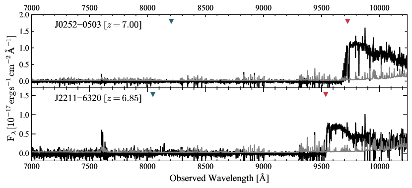
Figure 1: VLT/X-Shooter spectra of J0252–0503 and J2211–6320 in the observed wavelength. The original spectrum is shown by the black line, and spectral uncertainty is in gray. The observed wavelengths of Ly$\alpha$ and Ly$\beta$ emission lines are denoted by the red and blue triangles, respectively. Both spectra are smoothed with a median filter of $5$ pixels for better visualization.

The spectra of the $53$ quasars used in this work include most of the spectra presented in McGreer et al. (2011, 2015) and in Yang et al. (2020a). The quasar sample in McGreer et al. (2011, 2015) includes 29 spectra of 22 quasars at $5.73<z<6.42$, obtained with Keck II Telescope/Echellette Spectrograph and Imager (ESI), Magellan Baade Telescope/Magellan Echellette (MagE) Spectrograph, Multi-Mirror Telescope (MMT)/Red Channel Spectrograph, and Vergy Large Telescope (VLT)/X-Shooter. The quasar sample in Yang et al. (2020a) includes 35 spectra of 32 quasars at $6.31<z<7.00$ obtained with VLT/X-Shooter, Keck II/DEep Imaging Multi-Object Spectrograph (DEIMOS), Keck I/Low Resolution Imaging Spectrometer (LRIS), Gemini/Gemini Multi-Object Spectrographs (GMOS), Large Binocular Telescope (LBT)/Multi-Object Double CCD Spectrographs (MODS), and MMT/BINOSPEC. For the data reduction of these spectra, we refer the reader to McGreer et al. (2011, 2015) and Yang et al. (2020a) for more details. In addition to the spectra in McGreer et al. (2011, 2015) and Yang et al. (2020a), we have also included new VLT/X-Shooter spectra for quasars J0252–0503 ($z=7.00$) and J2211–6320 ($z=6.84$) in our study, both taken in 2019, and an archival VLT/X-Shooter spectrum for a quasar J1120+0641 at $z=7.085$ (Mortlock et al., 2011), taken in 2011 (Barnett et al., 2017). For the new VLT/X-Shooter spectra of J0252-0503 and J2211-6320, we perform the data reduction for bias subtracting, flat-fielding, and flux calibration with PypeIt (Prochaska et al., 2020a, b), following the standard thread. We present these two VLT/X-Shooter spectra in Figure 1.

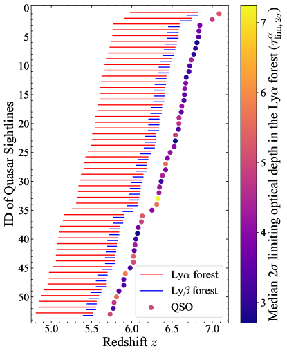
Figure 2: Redshift distribution of all quasars (circles) used in this study, and the redshift ranges of their Ly$\alpha$ (red lines) and Ly$\beta$ forests (blue lines) used in our analysis. The corresponding optical spectroscopic information of a quasar sightline ID can be found in Table 1. The median $2\sigma$ limiting optical depth in the Ly$\alpha$ forest ($\tau^{\alpha}_{\rm lim,2\sigma}$) of each quasar sightline is color-coded, calculated in Section 3, showing the average depth in the Ly$\alpha$ forest. A higher median $\tau^{\alpha}_{\rm lim,2\sigma}$ denotes that this quasar sightline is able to probe more opaque patches in the IGM.

We summarize the optical spectroscopy of all $53$ quasars in Table 1, in descending order of redshift. We show the redshift distribution of all quasars, and the redshift range of Ly$\alpha$ and Ly$\beta$ forests used in our data pixel fraction analysis in Figure 2.

For objects with multiple spectra, we use the histogram method to stack these spectra to improve the signal-to-noise ratio: we first set a common wavelength grid, based on the spectrum with lowest spectral resolution among all the spectra of the same object. Then we use the inverse variance weighting to calculate the flux, and the spectral uncertainty of each pixel on the common wavelength grid to obtain a stack spectrum.

For the range of the Ly$\alpha$ forest used in our analysis, we choose the blue cutoff at $1050~{}{\rm\AA}$ in the rest-frame to exclude the possible emission from O VI $\lambda$1033 (Bosman et al., 2021). We choose a red cutoff at $1176~{}{\rm\AA}$ in the rest-frame to avoid possible contamination from the quasar proximity zone. For the wavelength coverage of the Ly$\beta$ forest, we select a blue cutoff at $975~{}{\rm\AA}$ in the rest-frame to avoid contamination from Lyman $\gamma$ forests. We also match the red cut of the Ly$\beta$ forest to the same absorption redshift as the red cut of the Ly$\alpha$ forest (i.e., $1176~{}{\rm\AA}\times\lambda_{\rm Ly\beta}/\lambda_{\rm Ly\alpha}$ in the rest-frame, where $\lambda_{\rm Ly\alpha}=1215.7~{}{\rm\AA}$ and $\lambda_{\rm Ly\beta}=1025.7~{}{\rm\AA}$ are the rest wavelengths of Ly$\alpha$ and Ly$\beta$), resulting in a wavelength range of $975-992.2~{}{\rm\AA}$.

To minimize the contamination of strong sky emission lines (mainly ${\rm OH}$ emission) in our analysis, we first apply a median filter of 3 pixels to smooth the spectrum, and then mask pixels which are above $3\sigma$ in both flux density and spectral uncertainty than the smoothed spectrum. We reject pixels with SNR $<-5$ caused by oversubtraction of sky. Due to the sky ${\rm O}_{2}$ emission (Osterbrock et al., 1996), we also mask the SNR $>2$ pixels in the observed range of $8620-8680~{}{\rm\AA}$ range. This may exclude real transmission spikes, but SNR $>2$ pixels within this region cannot be identified as transmission spikes precisely, based on the current data quality. Eilers et al. (2019) showed that the metal absorption line contribution is negligible at $z\sim 6$, and we thus do not correct them in our analysis.

For some VLT/X-Shooter spectra in our study (especially at the high-redshift end), the sky background level is not precisely subtracted, resulting in a “zero” flux offset in these spectra. This flux floor is removed empirically as follows: after skyline masking, we first investigate the flux distribution of pixels in the Ly$\alpha$ forest. Then we perform $2\sigma$ sigma-clipping on the pixel flux until convergence of the mean and the median flux is achieved. Figure 3 shows the flux distribution of pixels in the Ly$\alpha$ forest as the black histogram from the J1120+0641 VLT/X-Shooter spectrum. The median flux from the sigma-clipped pixels is denoted by the vertical dashed line, and the $2\sigma$ range from the sigma clipping is represented by the grey shaded region. We use the median flux of sigma-clipped pixels to correct the zero flux level for all VLT/X-Shooter spectra of quasars. The average flux correction in transmitted flux is $\sim 0.08\%-4\%$.

Table 1: Information of Quasar Optical Spectroscopy

ID	Name	$z$	Telescope/Instrument	Median $\tau^{\alpha}_{\rm lim,2\sigma}$
1	J1120+0641	7.09	VLT/X-Shooter	5.23
2	J0252–0503	7.00	VLT/X-Shooter	4.76
3	J2211–6320	6.84	VLT/X-Shooter	3.73
4	J0020–3653	6.83	VLT/X-Shooter	3.77
5	J0319–1008	6.83	Gemini/GMOS	3.40
6	J0411–0907	6.81	LBT/MODS	2.78
7	J0109–3047	6.79	VLT/X-Shooter	3.05
8	J0218+0007	6.77	Keck/LRIS	2.95
9	J1104+2134	6.74	Keck/LRIS	4.33
10	J0910+1656	6.72	Keck/LRIS	3.34
11	J0837+4929	6.71	LBT/MODS	3.19
			MMT/BINOSPEC
12	J1048–0109	6.68	VLT/X-Shooter	3.00
13	J2002–3013	6.67	Gemini/GMOS	3.98
14	J2232+2930	6.66	VLT/X-Shooter	4.04
15	J1216+4519	6.65	Gemini/GMOS	3.49
			Keck/LRIS
			LBT/MODS
16	J2102–1458	6.65	Keck/DEIMOS	3.36
17	J0024+3913	6.62	Keck/DEIMOS	4.08
18	J0305–3150	6.61	VLT/X-Shooter	3.48
19	J1526–2050	6.59	Keck/DEIMOS	4.56
20	J2132+1217	6.59	Keck/DEIMOS	4.71
21	J1135+5011	6.58	MMT/BINOSPEC	3.39
22	J0226+0302	6.54	Keck/DEIMOS	4.81
23	J0148–2826	6.54	Gemini/GMOS	2.73
24	J0224–4711	6.53	VLT/X-Shooter	3.98
25	J1629+2407	6.48	Keck/DEIMOS	4.20
26	J2318–3113	6.44	VLT/X-Shooter	3.93
27	J1148+5251	6.42	Keck/ESI	5.60
28	J0045+0901	6.42	Keck/DEIMOS	3.89
29	J1036–0232	6.38	Keck/DEIMOS	4.45
30	J1152+0055	6.36	VLT/X-Shooter	3.11
31	J1148+0702	6.34	VLT/X-Shooter	4.20
32	J0142–3327	6.34	VLT/X-Shooter	4.28
33	J0100+2802	6.33	VLT/X-Shooter	7.25
34	J1030+0524	6.31	Keck/ESI	5.64
			VLT/X-Shooter
35	J1623+3112	6.25	Keck/ESI	3.95
36	J1319+0950	6.13	VLT/X-Shooter	5.27
37	J1509–1749	6.12	Magellan/MagE	4.92
			VLT/X-Shooter
38	J0842+1218	6.08	Keck/ESI	3.75
39	J1630+4012	6.07	MMT/Red Channel Spectrograph	2.71
40	J0353+0104	6.05	Keck/ESI	3.15
41	J2054–0005	6.04	Magellan/MagE	4.29
42	J1137+3549	6.03	Keck/ESI	3.45
43	J0818+1722	6.02	MMT/Red Channel Spectrograph	5.42
			VLT/X-Shooter
44	J1306+0356	6.02	Keck/ESI	5.04
			VLT/X-Shooter
45	J0841+2905	5.98	Keck/ESI	3.13
46	J0148+0600	5.92	VLT/X-Shooter	5.80
47	J1411+1217	5.90	Keck/ESI	3.37
48	J1335+3533	5.90	Keck/ESI	3.22
49	J0840+5624	5.84	Keck/ESI	3.52
50	J0836+0054	5.81	Keck/ESI	5.56
			MMT/Red Channel Spectrograph
			VLT/X-Shooter
51	J1044–0125	5.78	Magellan/MagE	4.74
52	J0927+2001	5.77	Keck/ESI	3.32
53	J1420–1602	5.73	Magellan/MagE	4.96

Note. — (1) ID of quasar sightlines, in descending order of redshift. (2) Name of quasar. (3) Redshift. (4) Instrument used to obtain the spectrum. (5) The median of $2\sigma$ limiting optical depth in the Ly$\alpha$ forest, on a pixel scale of $3.3~{}{\rm cMpc}$. If there are multiple spectra of one object, the listed $2\sigma$ limiting optical depth is given for the stacked spectrum.

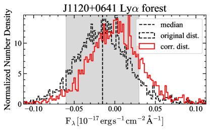
Figure 3: To correct “zero” flux level in VLT/X-Shooter spectra, we apply the median flux derived from sigma clipped pixels to the VLT/X-Shooter spectra. The original flux distribution of pixels in the Ly$\alpha$ forest from the J1120+0641 VLT/X-Shooter spectrum is shown by the black histogram. The median derived from the sigma clipping is denoted by the vertical black dashed line, and the 2$\sigma$ range from sigma clipping is in the grey shaded region. The flux distribution corrected by the sigma-clipped median is shown by the red histogram.

3 Methods

To improve the dynamic range of the spectrum, we follow a similar method as the method described in McGreer et al. (2011) to perform spectral binning. The size of each binned pixel is $3.3~{}{\rm Mpc}$ in the comoving distance (i. e., $3.3~{}{\rm cMpc}$), following McGreer et al. (2011, 2015). To avoid any contamination caused by residual sky lines in the spectrum, we first identify the local minima in the $1\sigma$ spectral uncertainty in the Ly$\alpha$ and Ly$\beta$ forests with argrelextrema in Scipy (Virtanen et al., 2020) and an order of 3, which identifies those local minima that are less than their 3 neighboring pixels in the spectral uncertainty. We place the $3.3~{}{\rm cMpc}$ pixels centered at those local minima, until the interval between any two adjacent pixels is less than $3.3~{}{\rm cMpc}$. We then use the inverse variance weighting to calculate the flux and the spectral uncertainty of each $3.3~{}{\rm cMpc}$ binned pixel. As an example, Figure 4 shows the J1120+0641 binned spectrum, corrected with the $2\sigma$ clipping median of all pixels. Before calculating the covering fraction of dark pixels, we perform a visual inspection on every binned spectrum by comparing it with near-infrared sky OH emission lines (Rousselot et al., 2000). We manually mask any bright pixel plausibly caused by sky emission at $z>6.3$ in the binned spectrum. These manually masked “sky” pixels are denoted by yellow hatched pixels in Figure 4.

We adopt a flux threshold method to identify “dark pixels” in the binned spectra, following McGreer et al. (2011). Pixels with flux density less than $2\sigma$, where $\sigma$ is the binned spectral uncertainty, are identified as “dark pixels”. These dark pixels are denoted by black bars in Figure 4. McGreer et al. (2011, 2015) introduced an alternative definition of the “dark” pixel fraction, as twice the fraction of pixels with negative flux. Since the “dark” pixels intrinsically have zero flux, there is a probability of $0.5$ for them to scatter below $0$ flux. We do not adopt this negative flux pixel definition, because this method requires an extremely precise background subtraction, which is difficult to achieve for the highest redshift quasar spectra in this study due to the sky background (see Section 2). As dark pixel fractions are used as upper limits on $\overline{x}_{\rm HI}$, we then calculate the ratio of total number of dark pixels to the total number of pixels of all quasar lines of sight as the dark pixel fraction, within a redshift bin of $\Delta z=0.2$, for both the Ly$\alpha$ transition (from $z=5.2$ to $z=6.8$) and the Ly$\beta$ transition (from $z=5.4$ to $z=6.8$). In each redshift bin, we use jackknife statistics to derive the $1\sigma$ uncertainty in the dark pixel fraction.

Apart from the individual constraints from Ly$\alpha$ and Ly$\beta$ forests, we also derive a combined dark pixel fraction in Ly$\alpha$ and Ly$\beta$ forests from their redshift overlapping regions (McGreer et al., 2011). For this combined dark pixel fraction, we stack the spectral uncertainty in Ly$\alpha$ and Ly$\beta$ forests at the same redshift using the inverse variance weighting, and utilize the stacked spectral uncertainty to put 3.3 cMpc pixels at local minima. The corresponding binned spectrum is shown on the lower middle panel in Figure 4. In this constraint, a pixel is “dark” only if its flux density is below $2\sigma$ binned spectral uncertainty in the both Ly$\alpha$ and Ly$\beta$ transitions. The redshift range used to calculate the dark pixel fraction for this combining constraints from Ly$\alpha$ and Ly$\beta$ forests is the same as the redshift range used to calculate the dark pixel fraction in Ly$\beta$ forests.

We perform a continuum fitting of the original spectrum by assuming a broken power-law with a break at the rest-frame 1000$~{}{\rm\AA}$ (Shull et al., 2012). We use the least square method to fit the spectrum within $1245-1285~{}{\rm\AA}$ and $1310-1380~{}{\rm\AA}$ in the rest-frame with a fixed spectral index ($\alpha_{\lambda}$) of $-1.5$, following Yang et al. (2020a), and derive the normalization of the power-law continuum. We then calculate the continuum flux at rest-frame $\lambda>1000~{}{\rm\AA}$ with the best-fit normalization and a spectral index of $-1.5$. At rest-frame $\lambda<1000~{}{\rm\AA}$, we switch the spectral index to $\alpha_{\lambda}=-0.59$ to calculate the continuum flux.

We calculate the $2\sigma$ limiting optical depth $\tau_{\rm lim,2\sigma}=-{\rm ln}(2\sigma/F_{\rm cont})$ for each $3.3~{}$cMpc pixel where $2\sigma$ is the binned uncertainty on a pixel size of $3.3~{}$cMpc, and $F_{\rm cont}$ is the best-fit continuum flux. A higher limiting optical depth indicates that the pixel can place stronger constraints on the neutral hydrogen fraction in the IGM. We present the median limiting optical depth in the Ly$\alpha$ forest of the binned spectra (on a pixel scale of $3.3~{}{\rm cMpc}$) in Table 1. For pixels in Ly$\beta$ forests, we correct their limiting optical depth by subtracting the effective optical depth of foreground Ly$\alpha$ forests, using the measured Ly$\alpha$ effective optical depth relations in Fan et al. (2006, for foreground Ly$\alpha$ forests at $z<5.3$) and in Yang et al. (2020a, for foreground Ly$\alpha$ forests at $5.3<z<6.0$). When calculating the dark pixel fraction, we exclude $\tau_{\rm lim,2\sigma}<2.5$ for Ly$\alpha$ pixels (i. e., $\tau^{\alpha}_{\rm lim,2\sigma}<2.5$), as those pixels do not have enough sensitivity to probe the neutral hydrogen. Considering the Ly$\alpha$ and Ly$\beta$ transitions have different oscillator strengths, the corresponding cut in a limiting optical depth for Ly$\beta$ pixels will be $\tau^{\beta}_{\rm lim,2\sigma}<2.50/2.19\sim 1.14$, assuming a conversion factor of $2.19$ between Ly$\alpha$ and Ly$\beta$ effective optical depth (Fan et al., 2006). Furthermore, we re-calculate the dark pixel fraction only with $\tau^{\alpha}_{\rm lim,2\sigma}>4.5$ pixels (corresponding to $\tau^{\beta}_{\rm lim,2\sigma}>2.05$ for Ly$\beta$ pixels) to constrain the neutral hydrogen fraction with high quality pixels.

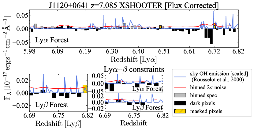
Figure 4: J1120+0641 binned spectrum in the Ly$\alpha$ forests (upper panel), Ly$\beta$ forests (lower left panel), and the redshift overlapping regions in Ly$\alpha$ and Ly$\beta$ forests (lower middle panel). The size of each binned pixel is $3.3~{}$cMpc. The binned $2\sigma$ spectral uncertainty is shown as the red line. The binned flux density is presented in bars, and identified “dark” pixels are shown in black. The sky OH emission is shown by the blue line (Rousselot et al., 2000), and our spectral binning method effectively puts the majority of pixels between sky OH emission lines. Yellow hatched pixels are manually masked during our analysis, as those fluxes are plausibly from residual sky OH emission. The zero flux level is corrected by the $2\sigma$ clipping median of all pixels in the Ly$\alpha$ forest (i. e., the vertical dashed line shown in Figure 3).

4 Results and Discussion

We present the redshift evolution of upper limits on $\overline{x}_{\rm HI}$ from dark pixels in Figure 5. The number of $\tau^{\alpha}_{\rm lim,2\sigma}>2.5$ pixels in each $\Delta z=0.2$ bin in redshift, the number of lines of sight in each redshift bin, and the upper limits derived from $\tau^{\alpha}_{\rm lim,2\sigma}>2.5$ pixels are shown in the left panel, and the results of $\tau^{\alpha}_{\rm lim,2\sigma}>4.5$ are shown in right panel. In both two panels, the combined dark pixel fractions from Ly$\alpha$ and Ly$\beta$ forests give the most stringent upper limits on $\overline{x}_{\rm HI}$. From the combined dark pixel fraction derived from $\tau^{\alpha}_{\rm lim,2\sigma}>2.5$ pixels in Ly$\alpha$ and Ly$\beta$ forests, the upper limit on the neutral hydrogen is $18\%\pm 8\%$ at $z=5.5$, and it increases to $69\%\pm 6\%$ at $z=6.1$, $79\%\pm 4\%$ at $z=6.3$, $87\%\pm 3\%$ at $z=6.5$, and $94\%_{-9\%}^{+6\%}$ at $z=6.7$. By adopting a higher limiting optical depth cut at $4.5$ than at $2.5$, the number of available pixels and the number of available quasar lines of sight drop significantly in each $\Delta z=0.2$ redshift bin. Furthermore, the upper limit on $\overline{x}_{\rm HI}$ becomes tighter at $z<6$. The upper limit on $\overline{x}_{\rm HI}$ is $9\%\pm 8\%$ at $z=5.5$, $16\%\pm 14\%$ at $z=5.7$, and $28\%\pm 8\%$ at $z=5.9$. At $z>6$, dark pixel fractions derived from $\tau^{\alpha}_{\rm lim,2\sigma}>4.5$ pixels increase significantly, which can be caused by the rapid evolution in the IGM Ly$\alpha$ and Ly$\beta$ effective optical depth (e.g.,  Yang et al., 2020a). However, this rapid increase in the combined Ly$\alpha$ and Ly$\beta$ dark pixel fraction can also be associated with a small data sample, as only $5$ quasar lines of sight are available with $\tau^{\alpha}_{\rm lim,2\sigma}>4.5$ pixels at $z=6.1$. Furthermore, at $z>6$, dark pixel fractions derived from $\tau^{\alpha}_{\rm lim,2\sigma}>4.5$ pixels do not necessarily provide more stringent upper limits on $\overline{x}_{\rm HI}$ than those derived from $\tau^{\alpha}_{\rm lim,2\sigma}>2.5$ pixels. At $z>6.3$, the number of available $\tau^{\alpha}_{\rm lim,2\sigma}>4.5$ pixels is very limited. For example, at $z\sim 6.4-6.6$ (the central redshift of the bin is $z=6.5$), there is no $\tau^{\alpha}_{\rm lim,2\sigma}>4.5$ pixel in Ly$\beta$ forests, due to the lack of high signal-to-noise ratio quasar spectra and the narrow wavelength range of Ly$\beta$ forests used in our analysis. We tabulate the redshift distributions of the number of quasar lines of sight, the number dark pixels, the number of pixels, and the value of dark pixel fractions in Table 2.

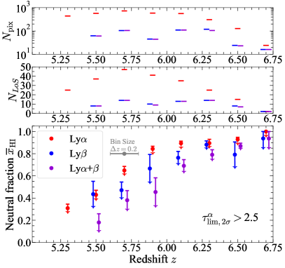
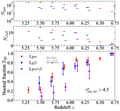
Figure 5: Upper Panels – Number of $3.3~{}$cMpc pixels used to calculate the dark pixel fraction in the Ly$\alpha$ (red), Ly$\beta$ (blue) forests and the combined dark fraction in the Ly$\alpha$ and Ly$\beta$ forests (purple) in each bin of $\Delta z=0.2$ in redshift; Middle Panels – Number of quasar lines of sight available in each bin of $\Delta z=0.2$ in redshift; Bottom Panels – Upper limits on the volume-averaged IGM neutral fraction $\overline{x}_{\rm HI}$ derived from the dark pixel fractions in the Ly$\alpha$ (red) and Ly$\beta$ (blue) forests as a function of redshift. The combined dark pixel fractions from the Ly$\alpha$ and Ly$\beta$ forests are denoted by purple markers. We adopt the same redshift bin ranges when calculating the dark pixel fractions derived from Ly$\alpha$ forests (red), Ly$\beta$ forests (blue), and combined Ly$\alpha$ and Ly$\beta$ forests (purple), but here we apply a small offset ${\Delta}z=0.02$ in the figure for better visualization. The three panels on the left show the results with $3.3~{}$cMpc pixels of which the limiting optical depth is greater than $2.5$; Three panels on the right are the results with $3.3~{}$cMpc pixels of which the limiting optical depth is greater than $4.5$. Note there is no $\tau^{\alpha}_{\rm lim,2\sigma}>4.5$ pixel in the Ly$\beta$ forest in the $z=6.5$ bin.

Table 2: Redshift distribution of the numbers of quasar lines of sight, of dark pixels, of all pixels, and resulting dark pixel fractions

Constraints	Redshift $z$	$\tau^{\alpha}_{\rm lim,2\sigma}>2.5$ pixels				$\tau^{\alpha}_{\rm lim,2\sigma}>4.5$ pixels
		$N_{\rm LoS}$	$N_{\rm dark}$	$N_{\rm pix}$	$f_{\rm dark}$	$N_{\rm LoS}$	$N_{\rm dark}$	$N_{\rm pix}$	$f_{\rm dark}$
(1)	(2)	(3)	(4)	(5)	(6)	(7)	(8)	(9)	(10)
Ly$\alpha$	5.3	25	135	437	$0.31\pm 0.04$	11	44	203	$0.22\pm 0.06$
	5.5	37	244	569	$0.43\pm 0.04$	14	49	218	$0.22\pm 0.05$
	5.7	47	472	727	$0.65\pm 0.04$	12	102	207	$0.49\pm 0.08$
	5.9	41	492	583	$0.84\pm 0.02$	11	79	111	$0.71\pm 0.05$
	6.1	35	498	557	$0.89\pm 0.02$	10	100	115	$0.87\pm 0.04$
	6.3	25	273	305	$0.90\pm 0.03$	5	40	48	$0.83\pm 0.08$
	6.5	15	118	127	$0.93\pm 0.02$	3	33	37	$0.89\pm 0.02$
	6.7	2	24	24	$1.00$	2	15	15	$1.00$
Ly$\beta$	5.5	8	27	62	$0.44\pm 0.12$	6	17	47	$0.36\pm 0.14$
	5.7	14	49	104	$0.47\pm 0.07$	10	27	67	$0.40\pm 0.10$
	5.9	10	30	45	$0.67\pm 0.13$	8	29	43	$0.67\pm 0.13$
	6.1	13	84	110	$0.76\pm 0.06$	10	54	74	$0.73\pm 0.06$
	6.3	14	104	118	$0.88\pm 0.03$	8	37	46	$0.80\pm 0.06$
	6.5	8	19	24	$0.79\pm 0.11$	0	0	0	$-$
	6.7	2	15	16	$0.94^{+0.06}_{-0.09}$	1	1	1	$1.00$
Combined Ly$\alpha+$Ly$\beta$	5.5	8	11	61	$0.18\pm 0.08$	4	3	35	$0.09\pm 0.08$
	5.7	14	40	105	$0.38\pm 0.09$	5	6	37	$0.16\pm 0.14$
	5.9	9	20	44	$0.45\pm 0.13$	4	7	25	$0.28\pm 0.08$
	6.1	13	76	110	$0.69\pm 0.06$	5	28	38	$0.74\pm 0.12$
	6.3	14	83	105	$0.79\pm 0.04$	3	13	21	$0.62\pm 0.16$
	6.5	7	20	23	$0.87\pm 0.03$	0	0	0	$-$
	6.7	2	15	16	$0.94^{+0.06}_{-0.09}$	1	1	1	$1.00$

Note. — (1) Type of dark pixel fractions. (2) Central redshift of each $\Delta z=0.2$ bin. (3) The number of quasar lines of sight that have $\tau^{\alpha}_{\rm lim,2\sigma}>2.5$ pixels in this redshift bin. (4) The number of $\tau^{\alpha}_{\rm lim,2\sigma}>2.5$ dark pixels. (5) The total number of $\tau^{\alpha}_{\rm lim,2\sigma}>2.5$ pixels. (6) Dark pixel fraction derived from $\tau^{\alpha}_{\rm lim,2\sigma}>2.5$ pixels. (7) The number of quasar lines of sight that have $\tau^{\alpha}_{\rm lim,2\sigma}>4.5$ pixels in this redshift bin. (8) The number of $\tau^{\alpha}_{\rm lim,2\sigma}>4.5$ dark pixels. (9) The total number of $\tau^{\alpha}_{\rm lim,2\sigma}>4.5$ pixels. (10) Dark pixel fraction derived from $\tau^{\alpha}_{\rm lim,2\sigma}>4.5$ pixels. All the errors show $1\sigma$ confidence intervals.

We show our upper limits on the IGM neutral hydrogen fraction, along with other constraints on neutral hydrogen fractions from high-redshift quasars in Figure 6. Since the dark pixel fraction derived from $\tau^{\alpha}_{\rm lim,2\sigma}>4.5$ pixels can provide tighter constraints on the neutral hydrogen fraction at $z<6$, and at $z>6$ the number of $\tau^{\alpha}_{\rm lim,2\sigma}>2.5$ pixels is much higher than the number of $\tau^{\alpha}_{\rm lim,2\sigma}>4.5$ pixels, we present the dark pixel fraction derived from $\tau^{\alpha}_{\rm lim,2\sigma}>2.5$ pixels at $z>6$, denoted by red upper limits. The dark pixel fraction calculated with $\tau^{\alpha}_{\rm lim,2\sigma}>4.5$ pixels at $z<6$ are denoted by magenta upper limits. The dark pixel fraction in McGreer et al. (2015) at $5.5<z<6.2$, derived from $22$ quasars are shown by blue upper limits. Our upper limits on the neutral fraction at $z<6$ are slightly higher than the upper limits in McGreer et al. (2015). The possible reasons for this difference include: (1) McGreer et al. (2015) double the covering fraction of negative pixels as the dark pixel fraction, while the dark pixel in this work is defined by $2\sigma$ flux threshold (McGreer et al., 2011), and (2) to avoid possible contamination from quasar proximity zones and intrinsic spectra, we adopt narrower wavelength ranges for both Ly$\alpha$ forests than the wavelength ranges used in McGreer et al. (2015). We repeat the results in McGreer et al. (2015) and test the above two factors in the resulted dark pixel fractions. We notice that the dark pixel definition (either dark pixels are defined by flux threshold or negative pixels) accounts for the major difference between our results and McGreer et al. (2015). Adopting a dark pixel definition of $2\sigma$ flux threshold, the combined Ly$\alpha$ and Ly$\beta$ dark pixel fractions in McGreer et al. (2015) will become $0.16\pm 0.08$ at $z=5.58$, $0.31\pm 0.10$ at $z=5.87$, and $0.63\pm 0.24$ at $z=6.07$, derived from $\tau^{\alpha}_{\rm lim,1\sigma}>4.5$ (corresponding $\tau^{\alpha}_{\rm lim,2\sigma}>3.8$) pixels. Although flux threshold definition gives more conservative dark pixel fractions at $z<6$, it is the only applicable method when deriving dark pixel fractions at the high-redshift end in this study, due to the strong sky emission.

In Figure 6, we show the upper limits on $\overline{x}_{\rm HI}$ from long dark gap size distributions in Ly$\alpha$ and Ly$\beta$ forests (Zhu et al., 2022), assuming a late reionization that ends at $z\lesssim 5.3$ (Nasir & D’Aloisio, 2020). Our constraints at $z<6$ are highly consistent with these upper limits derived from dark gap statistics. We also present constraints on $\overline{x}_{\rm HI}$ measured from the Ly$\alpha$ effective optical depth (Fan et al., 2006; Yang et al., 2020a; Bosman et al., 2021). These $\overline{x}_{\rm HI}$ measurements from Ly$\alpha$ effective optical depth suggest the IGM is highly ionized and $\overline{x}_{\rm HI}\lesssim 10^{-4}$ at $z<5.5$. At $z>6$, the Ly$\alpha$ effective optical depth measurements show that $\overline{x}_{\rm HI}\gtrsim 10^{-4}$ (Yang et al., 2020a). The IGM damping wing feature embedded in the $z>7$ quasar spectra can be used to constrain the IGM neutral fraction, based on models of the IGM morphology and quasar intrinsic emission (e. g.,  Schroeder et al., 2013). In Figure 6, we show several recent measurements on neutral fraction at $z>7$ from IGM damping wings in hexagons (Greig et al., 2017; Bañados et al., 2018; Davies et al., 2018; Greig et al., 2019; Wang et al., 2020; Yang et al., 2020b; Greig et al., 2022). Their medians show $\overline{x}_{\rm HI}\sim 0.2-0.7$, suggesting that the IGM is significantly neutral at $z\gtrsim 7$.

The reionization history, derived from Planck 2018 results, assuming the FlexKnot model (Planck Collaboration et al., 2020), is shown by the dark grey shaded region ($1\sigma$ confidence level), and the light grey shaded region ($2\sigma$ confidence level). The FlexKnot model reconstructs the reionization history with arbitrary number of knots, interpolates the reionization history between knots, and utilizes the Bayesian interference to marginalize the number of knots (Millea & Bouchet, 2018). We also include $1\sigma$ reionization histories from Robertson et al. (2015, red region), Finkelstein et al. (2019, blue region), and Naidu et al. (2020, purple region). The ionizing budget during reionization is dominated by faint galaxies ($M_{\rm UV}>-15$) in Finkelstein et al. (2019), while the reionization photon budget in the models of Robertson et al. (2015) and Naidu et al. (2020) is dominated by bright galaxies. Our upper limits on neutral hydrogen fraction at $6.3\lesssim z\lesssim 6.7$ are within the $1\sigma$ reionization history (assuming FlexKnot model) from Planck 2018. However, the upper limits on $\overline{x}_{\rm HI}$ derived from dark pixels are not very efficient in distinguishing the other three reionization histories at $z>6$ shown in Figure 6. This results from the limited number of quasar sight lines at $z>6.8$, and the noisy sky background in the observed wavelength of interest, leading to a small number of pixels with high limiting optical depth at $z\gtrsim 6.5$. Deeper optical spectroscopy on existing $z>6.8$ quasars and more quasar lines of sight at $z>6.8$, as well as potential observations from space, are needed for future similar studies to generate more stringent constraints on $\overline{x}_{\rm HI}$ at $z>6.5$.

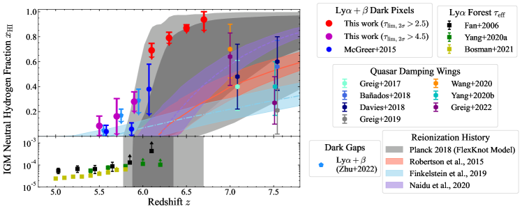
Figure 6: Constraints on the IGM neutral hydrogen fraction $\overline{x}_{\rm HI}$ from high-$z$ quasars studies and Planck 2018 results. The upper limits on $\overline{x}_{\rm HI}$ from dark pixels are in red (this work, derived from flux-corrected $\tau^{\alpha}_{\rm lim,2\sigma}>2.5$ pixels at $z>6$), magenta (this work, derived from flux-corrected $\tau^{\alpha}_{\rm lim,2\sigma}>4.5$ pixels at $z<6$), and blue (McGreer et al., 2015). Constraints on $\overline{x}_{\rm HI}$ derived from Ly$\alpha$ effective optical depth are shown by black squares (Fan et al., 2006), green squares (Yang et al., 2020a), and yellow squares (Bosman et al., 2021). The upper limits on $\overline{x}_{\rm HI}$, inferred from long dark gap length distributions in Ly$\alpha$ and Ly$\beta$ forests, are shown in blue pentagons (Zhu et al., 2022). At $z>7$, individual measurements on the neutral hydrogen fraction from quasar damping wings are denoted by hexagons (Greig et al., 2017; Bañados et al., 2018; Davies et al., 2018; Greig et al., 2019; Wang et al., 2020; Yang et al., 2020b). The $1\sigma$ and $2\sigma$ reionization history derived from Planck 2018 results by assuming the FlexKnot model are denoted by the dark grey shaded region and the light grey shaded region (Planck Collaboration et al., 2020). The colored regions display $1\sigma$ reionization histories in Robertson et al. 2015 (red), Finkelstein et al. 2019 (blue), and Naidu et al. 2020 (purple).

5 Conclusion

In this paper, we present the dark pixel fractions in Ly$\alpha$ and Ly$\beta$ forests of $53$ quasars at $5.73<z<7.09$. These dark pixel fractions provide the first model-independent upper limits on the volume-averaged IGM neutral fraction at $6.2<z<6.8$: $\overline{x}_{\rm HI}(z=6.3)<0.79\pm 0.04$ (1$\sigma$), $\overline{x}_{\rm HI}(z=6.5)<0.87\pm 0.03$ (1$\sigma$), and $\overline{x}_{\rm HI}(z=6.7)<0.94^{+0.06}_{-0.09}$ (1$\sigma$). The dark pixel fractions at $z<6.1$ in this work are slightly higher than the dark pixel fractions presented in McGreer et al. (2015), due to a different definition of dark pixels used in this work and the selection of different wavelength ranges in Lyman series forests for dark pixel fraction calculation. We find that the dark pixel fractions at $z>6.2$ are consistent with the $1\sigma$ IGM neutral fraction evolution derived from the Planck 2018 results when assuming the FlexKnot model (Planck Collaboration et al., 2020).

The current upper limits on $\overline{x}_{\rm HI}$, derived from dark pixels, are not stringent enough to distinguish various reionization histories (e.g.,  Robertson et al., 2015; Finkelstein et al., 2019; Naidu et al., 2020). The future improvement of similar dark pixel studies requires more quasar sightlines, deeper optical spectroscopy covering Lyman series forests, and observations from space to exclude the potential contamination from sky OH emission lines.

References

- Astropy Collaboration et al. (2013) Astropy Collaboration, Robitaille, T. P., Tollerud, E. J., et al. 2013, A&A, 558, A33, doi: 10.1051/0004-6361/201322068
- Astropy Collaboration et al. (2018) Astropy Collaboration, Price-Whelan, A. M., Sipőcz, B. M., et al. 2018, AJ, 156, 123, doi: 10.3847/1538-3881/aabc4f
- Astropy Collaboration et al. (2022) Astropy Collaboration, Price-Whelan, A. M., Lim, P. L., et al. 2022, apj, 935, 167, doi: 10.3847/1538-4357/ac7c74
- Bañados et al. (2018) Bañados, E., Venemans, B. P., Mazzucchelli, C., et al. 2018, Nature, 553, 473, doi: 10.1038/nature25180
- Barnett et al. (2017) Barnett, R., Warren, S. J., Becker, G. D., et al. 2017, A&A, 601, A16, doi: 10.1051/0004-6361/201630258
- Becker et al. (2015) Becker, G. D., Bolton, J. S., Madau, P., et al. 2015, MNRAS, 447, 3402, doi: 10.1093/mnras/stu2646
- Becker et al. (2021) Becker, G. D., D’Aloisio, A., Christenson, H. M., et al. 2021, MNRAS, 508, 1853, doi: 10.1093/mnras/stab2696
- Bosman et al. (2018) Bosman, S. E. I., Fan, X., Jiang, L., et al. 2018, MNRAS, 479, 1055, doi: 10.1093/mnras/sty1344
- Bosman et al. (2021) Bosman, S. E. I., Ďurovčíková, D., Davies, F. B., & Eilers, A.-C. 2021, MNRAS, 503, 2077, doi: 10.1093/mnras/stab572
- Calverley et al. (2011) Calverley, A. P., Becker, G. D., Haehnelt, M. G., & Bolton, J. S. 2011, MNRAS, 412, 2543, doi: 10.1111/j.1365-2966.2010.18072.x
- Carilli et al. (2010) Carilli, C. L., Wang, R., Fan, X., et al. 2010, ApJ, 714, 834, doi: 10.1088/0004-637X/714/1/834
- Davies et al. (2018) Davies, F. B., Hennawi, J. F., Bañados, E., et al. 2018, ApJ, 864, 142, doi: 10.3847/1538-4357/aad6dc
- Eilers et al. (2018) Eilers, A.-C., Davies, F. B., & Hennawi, J. F. 2018, ApJ, 864, 53, doi: 10.3847/1538-4357/aad4fd
- Eilers et al. (2017) Eilers, A.-C., Davies, F. B., Hennawi, J. F., et al. 2017, ApJ, 840, 24, doi: 10.3847/1538-4357/aa6c60
- Eilers et al. (2019) Eilers, A.-C., Hennawi, J. F., Davies, F. B., & Oñorbe, J. 2019, ApJ, 881, 23, doi: 10.3847/1538-4357/ab2b3f
- Fan et al. (2006) Fan, X., Strauss, M. A., Becker, R. H., et al. 2006, AJ, 132, 117, doi: 10.1086/504836
- Finkelstein et al. (2019) Finkelstein, S. L., D’Aloisio, A., Paardekooper, J.-P., et al. 2019, ApJ, 879, 36, doi: 10.3847/1538-4357/ab1ea8
- Greig et al. (2019) Greig, B., Mesinger, A., & Bañados, E. 2019, MNRAS, 484, 5094, doi: 10.1093/mnras/stz230
- Greig et al. (2022) Greig, B., Mesinger, A., Davies, F. B., et al. 2022, MNRAS, 512, 5390, doi: 10.1093/mnras/stac825
- Greig et al. (2017) Greig, B., Mesinger, A., Haiman, Z., & Simcoe, R. A. 2017, MNRAS, 466, 4239, doi: 10.1093/mnras/stw3351
- Harris et al. (2020) Harris, C. R., Millman, K. J., van der Walt, S. J., et al. 2020, Nature, 585, 357, doi: 10.1038/s41586-020-2649-2
- Hoag et al. (2019) Hoag, A., Bradač, M., Huang, K., et al. 2019, ApJ, 878, 12, doi: 10.3847/1538-4357/ab1de7
- Hunter (2007) Hunter, J. D. 2007, Computing in Science & Engineering, 9, 90, doi: 10.1109/MCSE.2007.55
- Itoh et al. (2018) Itoh, R., Ouchi, M., Zhang, H., et al. 2018, ApJ, 867, 46, doi: 10.3847/1538-4357/aadfe4
- Jung et al. (2020) Jung, I., Finkelstein, S. L., Dickinson, M., et al. 2020, ApJ, 904, 144, doi: 10.3847/1538-4357/abbd44
- Konno et al. (2014) Konno, A., Ouchi, M., Ono, Y., et al. 2014, ApJ, 797, 16, doi: 10.1088/0004-637X/797/1/16
- Konno et al. (2018) Konno, A., Ouchi, M., Shibuya, T., et al. 2018, PASJ, 70, S16, doi: 10.1093/pasj/psx131
- Mason et al. (2018) Mason, C. A., Treu, T., Dijkstra, M., et al. 2018, ApJ, 856, 2, doi: 10.3847/1538-4357/aab0a7
- Mason et al. (2019) Mason, C. A., Fontana, A., Treu, T., et al. 2019, MNRAS, 485, 3947, doi: 10.1093/mnras/stz632
- McGreer et al. (2015) McGreer, I. D., Mesinger, A., & D’Odorico, V. 2015, MNRAS, 447, 499, doi: 10.1093/mnras/stu2449
- McGreer et al. (2011) McGreer, I. D., Mesinger, A., & Fan, X. 2011, MNRAS, 415, 3237, doi: 10.1111/j.1365-2966.2011.18935.x
- Mesinger (2010) Mesinger, A. 2010, MNRAS, 407, 1328, doi: 10.1111/j.1365-2966.2010.16995.x
- Millea & Bouchet (2018) Millea, M., & Bouchet, F. 2018, A&A, 617, A96, doi: 10.1051/0004-6361/201833288
- Miralda-Escudé (1998) Miralda-Escudé, J. 1998, ApJ, 501, 15, doi: 10.1086/305799
- Morales et al. (2021) Morales, A. M., Mason, C. A., Bruton, S., et al. 2021, ApJ, 919, 120, doi: 10.3847/1538-4357/ac1104
- Mortlock et al. (2011) Mortlock, D. J., Warren, S. J., Venemans, B. P., et al. 2011, Nature, 474, 616, doi: 10.1038/nature10159
- Naidu et al. (2020) Naidu, R. P., Tacchella, S., Mason, C. A., et al. 2020, ApJ, 892, 109, doi: 10.3847/1538-4357/ab7cc9
- Nasir & D’Aloisio (2020) Nasir, F., & D’Aloisio, A. 2020, MNRAS, 494, 3080, doi: 10.1093/mnras/staa894
- Osterbrock et al. (1996) Osterbrock, D. E., Fulbright, J. P., Martel, A. R., et al. 1996, PASP, 108, 277, doi: 10.1086/133722
- Ouchi et al. (2018) Ouchi, M., Harikane, Y., Shibuya, T., et al. 2018, PASJ, 70, S13, doi: 10.1093/pasj/psx074
- Pentericci et al. (2011) Pentericci, L., Fontana, A., Vanzella, E., et al. 2011, ApJ, 743, 132, doi: 10.1088/0004-637X/743/2/132
- Planck Collaboration et al. (2020) Planck Collaboration, Aghanim, N., Akrami, Y., et al. 2020, A&A, 641, A6, doi: 10.1051/0004-6361/201833910
- Prochaska et al. (2020a) Prochaska, J., Hennawi, J., Westfall, K., et al. 2020a, The Journal of Open Source Software, 5, 2308, doi: 10.21105/joss.02308
- Prochaska et al. (2020b) Prochaska, J. X., Hennawi, J., Cooke, R., et al. 2020b, pypeit/PypeIt: Release 1.0.0, v1.0.0, Zenodo, doi: 10.5281/zenodo.3743493
- Robertson et al. (2015) Robertson, B. E., Ellis, R. S., Furlanetto, S. R., & Dunlop, J. S. 2015, ApJ, 802, L19, doi: 10.1088/2041-8205/802/2/L19
- Rousselot et al. (2000) Rousselot, P., Lidman, C., Cuby, J. G., Moreels, G., & Monnet, G. 2000, A&A, 354, 1134
- Schenker et al. (2014) Schenker, M. A., Ellis, R. S., Konidaris, N. P., & Stark, D. P. 2014, ApJ, 795, 20, doi: 10.1088/0004-637X/795/1/20
- Schroeder et al. (2013) Schroeder, J., Mesinger, A., & Haiman, Z. 2013, MNRAS, 428, 3058, doi: 10.1093/mnras/sts253
- Shull et al. (2012) Shull, J. M., Stevans, M., & Danforth, C. W. 2012, ApJ, 752, 162, doi: 10.1088/0004-637X/752/2/162
- Sobacchi & Mesinger (2015) Sobacchi, E., & Mesinger, A. 2015, MNRAS, 453, 1843, doi: 10.1093/mnras/stv1751
- Stark et al. (2010) Stark, D. P., Ellis, R. S., Chiu, K., Ouchi, M., & Bunker, A. 2010, MNRAS, 408, 1628, doi: 10.1111/j.1365-2966.2010.17227.x
- Venemans et al. (2015) Venemans, B. P., Bañados, E., Decarli, R., et al. 2015, ApJ, 801, L11, doi: 10.1088/2041-8205/801/1/L11
- Virtanen et al. (2020) Virtanen, P., Gommers, R., Oliphant, T. E., et al. 2020, Nature Methods, 17, 261, doi: 10.1038/s41592-019-0686-2
- Wang et al. (2020) Wang, F., Davies, F. B., Yang, J., et al. 2020, ApJ, 896, 23, doi: 10.3847/1538-4357/ab8c45
- Worseck et al. (2014) Worseck, G., Prochaska, J. X., O’Meara, J. M., et al. 2014, MNRAS, 445, 1745, doi: 10.1093/mnras/stu1827
- Yang et al. (2020a) Yang, J., Wang, F., Fan, X., et al. 2020a, ApJ, 904, 26, doi: 10.3847/1538-4357/abbc1b
- Yang et al. (2020b) —. 2020b, ApJ, 897, L14, doi: 10.3847/2041-8213/ab9c26
- Zhu et al. (2021) Zhu, Y., Becker, G. D., Bosman, S. E. I., et al. 2021, ApJ, 923, 223, doi: 10.3847/1538-4357/ac26c2
- Zhu et al. (2022) —. 2022, ApJ, 932, 76, doi: 10.3847/1538-4357/ac6e60