Representations of the symmetric group are decomposable in polynomial time

Abstract

We introduce an algorithm to decompose orthogonal matrix representations of the symmetric group over the reals into irreducible representations, which as a by-product also computes the multiplicities of the irreducible representations. The algorithm applied to a $d$-dimensional representation of $S_{n}$ is shown to have a complexity of ${\mathcal{O}}(n^{2}d^{3})$ operations for determining multiplicities of irreducible representations and a further ${\mathcal{O}}(nd^{4})$ operations to fully decompose representations with non-trivial multiplicities. These complexity bounds are pessimistic and in a practical implementation using floating point arithmetic and exploiting sparsity we observe better complexity. We demonstrate this algorithm on the problem of computing multiplicities of two tensor products of irreducible representations (the Kronecker coefficients problem) as well as higher order tensor products. For hook and hook-like irreducible representations the algorithm has polynomial complexity as $n$ increases.

2020 Mathematics Subject Classification: 20C30, 65Y20.

1 Introduction

Let $\rho:S_{n}\rightarrow\hbox{\rm O}(d)$ be an orthogonal matrix representation of the symmetric group, acting on the vector space $V={\mathbb{R}}^{d}$. In other words $\rho$ is a homomorphism: for all $a,b\in S_{n}$ we have $\rho(ab)=\rho(a)\rho(b)$. We consider the problem of decomposing the representation into irreducible representations, that is decomposing

$$V\cong V_{1}^{\oplus a_{1}}\oplus\cdots\oplus V_{r}^{\oplus a_{r}}$$

where $\rho_{1},\ldots,\rho_{r}$ are each irreducible representations acting on the vector spaces $V_{1},\ldots,V_{r}$. We assume that we are given the generators of a representation of $S_{n}$ as symmetric (which must also be orthogonal) matrices $\rho(\tau_{1}),\ldots,\rho(\tau_{n-1})\in\hbox{\rm O}(d)$ where $\tau_{\ell}=(\ell\ (\ell+1))$ are the simple transpositions, i.e., the Coxeter generators.

We shall first consider the following fundamental problem:

Problem 1.

Given generators $\rho(\tau_{1}),\ldots,\rho(\tau_{n-1})\in\hbox{\rm O}(d)$ of an orthogonal matrix representation $\rho:S_{n}\rightarrow\hbox{\rm O}(d)$, determine the multiplicities $a_{1},\ldots,a_{r}$ of each irreducible representation, that is, how many times does each irreducible representation occur in the above decomposition.

We will then solve the question of decomposing a representation by solving an equivalent linear algebra problem:

Problem 2.

Given generators $\rho(\tau_{1}),\ldots,\rho(\tau_{n-1})\in\hbox{\rm O}(d)$ of an orthogonal matrix representation $\rho:S_{n}\rightarrow\hbox{\rm O}(d)$, compute an orthogonal matrix $Q\in\hbox{\rm O}(d)$ that block-diagonalises the representation so that

$$Q^{\top}\rho(g)Q=\begin{pmatrix}\rho_{1}(g)^{\oplus a_{1}}\\ &\ddots\\ &&\rho_{r}(g)^{\oplus a_{r}}\end{pmatrix}$$

where $\rho_{1},\ldots,\rho_{r}$ are distinct irreducible representations and $a_{1},\ldots,a_{r}$ are the multiplicities. Here we use the notation

$$\rho_{k}(g)^{\oplus a_{k}}=I_{a_{k}}\otimes\rho_{k}(g)=\begin{pmatrix}\rho_{k}(g)\\ &\ddots\\ &&\rho_{k}(g)\end{pmatrix}\in\hbox{\rm O}(d_{k}a_{k})$$

where $\rho_{k}(g)\in\hbox{\rm O}(d_{k})$ and $d_{k}$ is the dimension of the irreducible representation.

In this paper we will prove that both problems are computable (assuming real arithmetic). In particular, for an orthogonal matrix representation $\rho:S_{n}\rightarrow\hbox{\rm O}(d)$, Problem 1 can be solved via Algorithm 1 in ${\mathcal{O}}(n^{2}d^{3})$ operations (Corollary 2) and Problem 2 can be solved via Algorithm 2 in a further ${\mathcal{O}}(nd^{4})$ operations (Corollary 3).

Prior work on these problems begins with Dixon [3], who constructed an iterative algorithm for reducing representations of general finite groups to irreducible components, which can be used to solve Problem 1 in the limit. However, it does not consider the decomposition of repeated copies of irreducibles hence does not solve Problem 2, that is, it only computes the canonical representation as in [12]. Furthermore, the algorithm requires the computation of eigenvectors and eigenvalues which also depends on iterative algorithms which may fail. In other work, Serre [12, Theorem 8, Proposition 8] introduced projections to irreducible representations that lead to an effective algorithm, see [6] and related software [7]. However, the projections require computing a sum over every element of the group, that is, the complexity grows with the order of the group, factorially with $n$ for the symmetric group $S_{n}$. There is also related work on decomposing representations of compact groups [11].

Solving Problem 1 in the special case where the representation is a tensor products of irreducible representations of $S_{n}$ is one approach to computing Kronecker coefficients, a problem that is known to be NP-hard (in particular, $\#$P-hard [2]). In certain settings where the corresponding partitions have a fixed length there is a combinatorial algorithm that can compute specific Kronecker coefficients in polynomial time [10]. It is difficult to make a direct comparison between our complexity results when applied to the Kronecker coefficients problem: our complexity results depend on the dimension of the corresponding irreducible representations and we obtain all non-zero multiplicities without having to deduce the zero multiplicities, whereas the complexity results of [10] largely depend on the length of the corresponding partitions (including that of the partition determining the multiplicity being computed) and give no approach to deduce which multiplicities are nonzero apart from testing all possible partitions.

As a concrete example we will use throughout this paper, consider the representation coming from permutation matrices  $\rho^{\rm s}:S_{n}\rightarrow{\mathbb{R}}^{n\times n}$, where $\rho^{\rm s}(g)$ is the identity matrix $I_{n}$ with the rows permuted according to $g$. It has symmetric generators $\rho^{\rm s}(\tau_{\ell})$ with the $\ell$ and $(\ell+1)$th rows permuted. The permutation matrix representation of $S_{4}$ is block-diagonalised by the matrix

$$Q=\begin{pmatrix}1/\sqrt{2}&1/\sqrt{6}&1/\sqrt{12}&-1/2\cr-1/\sqrt{2}&1/\sqrt{6}&1/\sqrt{12}&-1/2\cr&-\sqrt{2/3}&1/\sqrt{12}&-1/2\cr&&-\sqrt{3}/2&-1/2\end{pmatrix}$$ (1)

A quick check shows that we have block-diagonalised the generators (and hence the representation) into $3\times 3$ and $1\times 1$ sub-blocks:

$$Q^{\top}\rho^{\rm s}(\tau_{1})Q\; =\begin{pmatrix}-1&&&\vline\\ &1&&\vline\\ &&1&\vline\\ \hline\cr&&&\vline&1\end{pmatrix},\quad Q^{\top}\rho^{\rm s}(\tau_{2})Q=\begin{pmatrix}1/2&\sqrt{3}/2&&\vline\\ \sqrt{3}/2&-1/2&&\vline\\ &&1&\vline\\ \hline\cr&&&\vline&1\end{pmatrix},$$

$$Q^{\top}\rho^{\rm s}(\tau_{3})Q\; =\begin{pmatrix}1&&&\vline\\ &1/3&2\sqrt{2}/3&\vline\\ &2\sqrt{2}/3&-1/3&\vline\\ \hline\cr&&&\vline&1\end{pmatrix}.$$

Note that the sub-blocks are necessarily also representations of $S_{4}$. That is, we have decomposed the permutation matrix representation into two irreducible representations both with unit multiplicity, one associated with the partition $(3,1)$ and the other with the trivial irreducible representation with partition $(4)$. The algorithms we introduce computes these partitions and multiplicities as well as the matrix $Q$ from the generators $\rho^{\rm s}(\tau_{1}),\rho^{\rm s}(\tau_{2}),\rho^{\rm s}(\tau_{3})$.

The paper is structured as follows:

Section 2: We review basics of representation theory of the symmetric group, including irreducible representations, their generators, the Gelfand–Tsetlin (GZ) algebra and its spectral properties for irreducible representations.

Section 3: We detail how the problem of reducing an orthogonal matrix representation can be recast as Problem 2.

Section 4: We discuss how the GZ algebra can be used to solve Problem 1 via a joint spectrum problem involving commuting symmetric matrices. This also gives a way to reduce a representation into irreducible representations but cannot distinguish multiple copies of the same irreducible representation, that is, we compute the canonical representation.

Section 5: We discuss how irreducible representations involving multiple copies of the same irreducible representation can be reduced, leading to the solution of Problem 2.

Section 6: We outline the algorithms for solving Problem 2 and Problem 1 and discuss briefly their practical implementation using floating point arithmetic.

Section 7: We show examples including tensor products of irreducible representations (the Clebsch–Gordan or Kronecker coefficients) and higher order analogues, using a floating-point arithmetic implementation of the proposed algorithm. We also demonstrate polynomial complexity for hook and hook-like irreducible representations.

Acknowledgments: I thank Oded Yacobi (U. Sydney) for significant help in understanding the basics of representation theory and in particular [8], as well as Peter Olver (U. Minnesota), Alex Townsend (Cornell), and Marcus Webb (U. Manchester) for helpful suggestions on drafts. This work was completed with the support of the EPSRC grant EP/T022132/1 “Spectral element methods for fractional differential equations, with applications in applied analysis and medical imaging” and the Leverhulme Trust Research Project Grant RPG-2019-144 “Constructive approximation theory on and inside algebraic curves and surfaces”.

2 Irreducible representations of the symmetric group

In this section we review some basic facts of representation theory of the symmetric group, roughly following [8]. The irreducible representations can be identified with partitions:

Definition 1.

A partition of $n$, is a tuple $\lambda=(\lambda_{1},\ldots,\lambda_{k})$ of integers $\lambda_{1}\geq\cdots\geq\lambda_{k}\geq 1$ such that $n=\lambda_{1}+\cdots+\lambda_{k}$. We use the notation $\lambda\vdash n$ to denote that $\lambda$ is a partition of $n$.

A basis for the vector space associated with an irreducible representation can be identified with Young tableaux:

Definition 2.

A Young tableau is a chain of partitions $(\lambda^{1},\ldots,\lambda^{n})$ where $\lambda^{j}\vdash j$ such that $\lambda^{j+1}$ is equivalent to $\lambda^{j}$ with one entry increased or one additional entry. The set of all Young tableaux of length $n$ is denoted ${\mathcal{Y}}_{n}$.

A natural way to visualise a partition is via a Young diagram: if $\lambda=(\lambda_{1},\ldots,\lambda_{k})$ then a Young diagram consists of $k$ rows of boxes where the $j$th row has exactly $\lambda_{j}$ boxes. A natural way to visualise a Young tableau is by filling in the boxes of a Young Diagram according to the order in which the new boxes appear in the sequence of Young Diagrams corresponding to $\lambda^{j}$. For example, the Young tableau $((1),(2),(2,1),(2,1,1),(2,2,1),(3,2,1),(3,2,1,1))$ can be depicted

$$1 6 3 5 4 7$$ (2)

The number of Young tableaux of a given partition $\lambda\vdash n$ is called the hook length $d_{\lambda}$. Young tableaux can be used to build an explicit irreducible matrix representation:

Definition 3.

Associated with any partition $\lambda$ is a canonical orthogonal matrix irreducible representation $\rho_{\lambda}:S_{n}\rightarrow\hbox{\rm O}(d_{\lambda})$. The dimension of the irreducible representation is the number of Young tableaux $d_{\lambda}$ and hence we can parameterise ${\mathbb{R}}^{d_{\lambda}}$ by an enumeration of Young tableaux $\left\{{y_{1},\ldots,y_{d_{\lambda}}}\right\}={\mathcal{Y}}_{n}$. The entries of the (symmetric) generators $\rho_{\lambda}(\tau_{\ell})$ are given by the following rules (cf. [8, (6.5)]):

1. For the Young tableau $y_{j}$, if box $\ell$ and $\ell+1$ are in the same row then $\mbox{\boldmath$e$\unboldmath}_{j}^{\top}\rho_{\lambda}(\tau_{\ell})\mbox{\boldmath$e$\unboldmath}_{j}=1$.

2. For the Young tableau $y_{j}$, if box $\ell$ and $\ell+1$ are in the same column then $\mbox{\boldmath$e$\unboldmath}_{j}^{\top}\rho_{\lambda}(\tau_{\ell})\mbox{\boldmath$e$\unboldmath}_{j}=-1$.

3. For the Young tableau $y_{j}$, if box $\ell$ and $\ell+1$ are not in the same row or column then let $k$ be such that $y_{k}$ is equal to $y_{j}$ except with boxes $\ell$ and $\ell+1$ swapped. If $(i_{\ell},j_{\ell})$ is the index of box $\ell$, then for the axial distance $r=j_{\ell+1}+i_{\ell}-i_{\ell+1}-j_{\ell}$ we have

   $$\mbox{\boldmath$e$\unboldmath}_{j}^{\top}\rho_{\lambda}(\tau_{\ell})\mbox{\boldmath$e$\unboldmath}_{j}\; =1/r,$$

   $$\mbox{\boldmath$e$\unboldmath}_{k}^{\top}\rho_{\lambda}(\tau_{\ell})\mbox{\boldmath$e$\unboldmath}_{j}\; =\sqrt{1-1/r^{2}}$$

4. All other entries are zero.

We now introduce the Gelfand–Tsetlin (GZ) algebra, which is a commutative algebra that we shall utilise to determine the multiplicities of the irreducible representations as well as decompose a representation into its canonical representation.

Definition 4.

The Young–Jucys–Murphy (YJM)-generators are

$$X_{1}\; =0,X_{2}=(1\ 2),X_{3}=(1\ 3)+(2\ 3),\ldots,X_{n}=(1\ n)+\cdots+(n-1\ n)$$

where $(i\ j)\in S_{n}$ is cyclic notation for the permutation that swaps $i$ and $j$.

The Gelfand–Tsetlin (GZ) algebra, a sub-algebra of the group algebra of $S_{n}$, is generated by the YJM generators [8, Corollary 2.6]: $\hbox{GZ}(n)=\left\langle{X_{1},\ldots,X_{n}}\right\rangle.$ Note that a representation $\rho:S_{n}\rightarrow\hbox{\rm O}(d)$ induces a representation $\rho:\hbox{GZ}(n)\rightarrow{\mathbb{R}}^{d\times d}$. We shall see that $\rho(X_{1}),\ldots,\rho(X_{n})$ are commuting matrices whose joint spectrum encodes Young tableaux, which in turn encodes the multiplicities of the irreducible representations. In particular, Young tableaux appear in the spectrum as content vectors:

Definition 5.

A content vector $\mbox{\boldmath$\alpha$\unboldmath}={\left({a_{1},\ldots,a_{n}}\right)}\in\hbox{\rm Cont}(n)\subset{\mathbb{Z}}^{n}$ satisfies the following:

1. $a_{1}=0$.

2. $\left\{{a_{k}-1,a_{k}+1}\right\}\cap\left\{{a_{1},\ldots,a_{k-1}}\right\}\neq \mathchar 0\relax$ for $k=2,\ldots,n$.

3. If $a_{k}=a_{j}=a$ for some $k<j$ then

   $$\left\{{a-1,a+1}\right\}\subset\left\{{a_{k+1},\ldots,a_{j-1}}\right\}.$$

There is a bijection between content vectors and Young Tableaux, [8, Proposition 5.3], which we denote $\hbox{\rm cont}:{\mathcal{Y}}_{n}\rightarrow\hbox{\rm Cont}(n)$. This map can be constructed as follows: if the box in the $i$-th row and $k$-th column in a Young tableau has the number $k$ in it then the $k$-th entry of the corresponding content vector is $j-i$. For example, for the Young diagram with partition $(3,2,1,1)$ the contents are

$0$ $2$ $-1$ $0$ $-2$ $-3$

and so the Young tableau in (2) would have corresponding content vector ${\left({0,1,-1,-2,0,2,-3}\right)}$. The map from content vectors to Young tableaux consists of filling in the boxes in the order the diagonals appear. In particular, if in the $k$th entry of the content vector we have an integer $p$ which has appeared $\mu$ times then, if $p$ is non-negative, the $(\mu+1,\mu+p+1)$ box is equal to $k$, otherwise, if $p$ is negative, the $(\mu-p+1,\mu+1)$ box is equal to $k$.

We now come to the key result: $\rho_{\lambda}(X_{j})$ are diagonal for all irreducible representations and their entries encode all content vectors associated with the corresponding partition. The following is equivalent to [8, Theorem 5.8]:

Lemma 1.

$\rho_{\lambda}(X_{j})$ is diagonal and the diagonal entries form a content vector: for each $k=1,\ldots,d_{\lambda}$

$${\begin{pmatrix}\mbox{\boldmath$e$\unboldmath}_{k}^{\top}\rho_{\lambda}(X_{1})\mbox{\boldmath$e$\unboldmath}_{k}\cr\vdots\cr{\mbox{\boldmath$e$\unboldmath}_{k}^{\top}\rho_{\lambda}(X_{n})\mbox{\boldmath$e$\unboldmath}_{k}}\cr\end{pmatrix}}=\hbox{\rm cont}(y_{k})$$

where $\left\{{y_{1},\ldots,y_{d_{\lambda}}}\right\}={\mathcal{Y}}_{n}$ are an enumeration of Young tableaux.

3 From representation theory to linear algebra

A classic result in representation theory is that all representations of finite groups are decomposable:

Proposition 1.

[4, Proposition 1.8] For any representation $\rho:G\rightarrow\hbox{\rm GL}(V)$ of a finite group $G$ there is a decomposition

$$V\cong V_{1}^{\oplus a_{1}}\oplus\cdots\oplus V_{r}^{\oplus a_{r}}$$

where the $\rho_{k}:G\rightarrow V_{i}$ are distinct irreducible representations. The decompositions of $V$ into a direct sum of the $r$ factors is unique, as are the $V_{k}$ that occur and their multiplicities $a_{k}$.

In terms of concrete linear algebra and specialising to the case of $G=S_{n}$ where we are given an orthogonal matrix representation $\rho:S_{n}\rightarrow\hbox{\rm O}(d)$, we denote the $a_{k}$ subspaces $V_{k}^{(1)},\ldots,V_{k}^{(a_{k})}\subset{\mathbb{R}}^{d}$ whose intersection is $\{0\}$ that are all isomorphic to $V_{k}={\mathbb{R}}^{d_{k}}$ where $d_{k}:=d_{\lambda^{k}}$ for $\lambda^{k}\vdash n$. Consider an orthogonal basis which spans $V_{k}^{(p)}$: if $V_{k}$ has dimension $d_{k}$ then let $B_{k}^{(p)}\in{\mathbb{R}}^{d\times d_{k}}$ with orthogonal columns (that is $(B_{k}^{(p)})^{\top}B_{k}^{(p)}=I_{d_{k}}$) such that $V_{k}^{(p)}=\hbox{\rm colspan}\,B_{k}^{(p)}$. Because $V_{k}^{(p)}$ are isomorphic to $V_{k}$, we know we can choose $B_{k}^{(p)}$ so that

$$\rho(g)B_{k}^{(p)}=B_{k}^{(p)}\rho_{k}(g)$$

where $\rho_{k}:=\rho_{\lambda^{k}}$. That is, we can choose the columns of $B_{k}^{(p)}$ so that the resulting representation is precisely of the form of Definition 3.

We shall use Schur’s Lemma to show that $\{B_{k}^{(p)}\}$ have certain orthogonality properties:

Lemma 2.

[4, Schur’s Lemma 1.7] If $\rho_{V}:G\rightarrow\hbox{\rm GL}(V)$ and $\rho_{W}:G\rightarrow\hbox{\rm GL}(W)$ are irreducible representations of $G$ and $\varphi:V\rightarrow W$ is a $G$-module homomorphism, then

1. Either $\varphi$ is an isomorphism, or $\varphi=0$.

2. If $\rho_{V}=\rho_{W}$, then $\varphi=cI$ for some $c\in{\mathbb{C}}$.

This lemma encodes the fact that bases corresponding to differing irreducible representations are automatically orthogonal to each other whereas bases corresponding to the same irreducible representation have inner products that are a scaled identity:

Corollary 1.

$$(B_{k}^{(p)})^{\top}B_{j}^{(q)}=\begin{cases}0_{d_{k}\times d_{j}}&k\neq j\\ m_{k}^{(pq)}I_{d_{k}}&k=j\end{cases}$$

for some constants $m_{k}^{(pq)}\in{\mathbb{R}}$.

Proof.

Consider the map $\varphi:{\mathbb{R}}^{d_{j}}\rightarrow{\mathbb{R}}^{d_{k}}$ defined by $\varphi(v):=(B_{k}^{(p)})^{\top}B_{j}^{(q)}v$. This is a $G$-module homomorphism:

$$\rho_{k}(g)\varphi(v)=(B_{k}^{(p)}\rho_{k}(g^{-1}))^{\top}B_{j}^{(q)}v=(\rho(g^{-1})B_{k}^{(p)})^{\top}B_{j}^{(q)}v=(B_{k}^{(p)})^{\top}B_{j}^{(q)}\rho_{j}(g)v=\varphi(\rho_{j}(g)v).$$

The corollary therefore follows from Schur’s lemma, where the fact that $m_{k}^{(pq)}$ is real follows since $B_{k}^{(p)},B_{j}^{(q)}$ have real entries. ∎

The previous proposition guarantees that if all irreducible representations have trivial multiplicity ($a_{1}=\cdots=a_{r}=1$) then $U={\begin{pmatrix}\,B_{1}^{(1)}\ |\ B_{2}^{(1)}\ |\ \ldots\ |\ B_{r}^{(1)}\,\end{pmatrix}}$ is an orthogonal matrix. This is not necessarily the case when we have non-trivial multiplicities. However, we can guarantee the existence of an orthogonal matrix that fully block-diagonalises a representation by taking an appropriate linear combination of $B_{k}^{(1)},\ldots,B_{k}^{(a_{k})}$, thus guaranteeing that Problem 2 has a solution:

Theorem 1.

There exists an orthogonal matrix $Q$ such that

$$Q^{\top}\rho(g)Q=\begin{pmatrix}\rho_{1}(g)^{\oplus a_{1}}\\ &\ddots\\ &&\rho_{r}(g)^{\oplus a_{r}}\end{pmatrix}$$

where $\rho_{1},\ldots,\rho_{r}$ are all irreducible representations.

Proof.

Recall $(B_{k}^{(p)})^{\top}B_{k}^{(q)}=m_{k}^{(pq)}I_{d_{k}}$ and consider the Cholesky decomposition

$$\underbrace{\begin{pmatrix}m_{k}^{(11)}&\cdots&m_{k}^{(1a_{k})}\\ \vdots&\ddots&\vdots\\ m_{k}^{(a_{k}1)}&\cdots&m_{k}^{(a_{k}a_{k})}\end{pmatrix}}_{M_{k}}=\tilde{R}_{k}^{\top}\tilde{R}_{k}.$$

Note that $\tilde{R}_{k}$ is invertible as $M_{k}$ is a Gram matrix (associated with the first columns of $B_{k}^{(1)},\ldots,B_{k}^{(a_{k})}$). Define $R_{k}=\tilde{R}_{k}\otimes I_{d_{k}}$ and $Q_{k}:={\begin{pmatrix}\,B_{k}^{(1)}\ |\ \ldots\ |\ B_{k}^{(a_{k})}\,\end{pmatrix}}R_{k}^{-1}$, which has orthogonal columns as $Q_{k}^{\top}Q_{k}=R_{k}^{-\top}(M_{k}\otimes I_{d_{k}})R_{k}^{-1}=I_{a_{k}d_{k}}$. We then have

$$\rho(g)Q_{k}\; ={\begin{pmatrix}\,B_{k}^{(1)}\ |\ \ldots\ |\ B_{k}^{(a_{k})}\,\end{pmatrix}}(I_{a_{k}}\otimes\rho_{k}(g))(\tilde{R}_{k}^{-1}\otimes I_{d_{k}})$$

$$={\begin{pmatrix}\,B_{k}^{(1)}\ |\ \ldots\ |\ B_{k}^{(a_{k})}\,\end{pmatrix}}(\tilde{R}_{k}^{-1}\otimes I_{d_{k}})(I_{a_{k}}\otimes\rho_{k}(g))=Q_{k}\rho_{k}(g)^{\oplus a_{k}}.$$

Thus $Q:={\begin{pmatrix}\,Q_{1}\ |\ \ldots\ |\ Q_{r}\,\end{pmatrix}}$ satisfies the necessary properties.

∎

4 Counting multiplicities via the Gelfand–Tsetlin algebra and basis

We now consider the solution of Problem 1: how do we use the existence of an orthogonal basis to determine how many copies of each irreducible representation are present in a given representation? The key will be the simultaneous diagonalisation of related commuting operators: the representations of the YJM-generators $\rho(X_{1}),\ldots,\rho(X_{n})$.

Let us return to the permutation matrix representation of $S_{4}$ example, where we have (omitting the triviality $\rho^{\rm s}(X_{1})=0$):

$$\rho^{\rm s}(X_{2})\; =\begin{pmatrix}0&1\cr 1&0\cr&&1\cr&&&1\end{pmatrix},\rho^{\rm s}(X_{3})=\begin{pmatrix}1&0&1\cr 0&1&1\cr 1&1&0\cr&&&2\end{pmatrix},\rho^{\rm s}(X_{4})=\begin{pmatrix}2&0&0&1\cr 0&2&0&1\cr 0&0&2&1\cr 1&1&1&0\end{pmatrix}.$$

Note the above are all symmetric matrices. In fact, they also commute. If we conjugate with the orthogonal matrix $Q$ from (1) that block-diagonalised the representation we have that the GZ generators are simultaneously diagonalised:

$$Q^{\top}\rho^{\rm s}(X_{1})Q\; =\hbox{\rm diag}(0,0,0,0),$$

$$Q^{\top}\rho^{\rm s}(X_{2})Q\; =\hbox{\rm diag}(-1,1,1,1),$$

$$Q^{\top}\rho^{\rm s}(X_{3})Q\; =\hbox{\rm diag}(1,-1,2,2),$$

$$Q^{\top}\rho^{\rm s}(X_{4})Q\; =\hbox{\rm diag}(2,2,-1,3).$$

This property is general:

Proposition 2.

If $\rho$ is an orthogonal matrix representation then $\rho(X_{1}),\ldots,\rho(X_{n})$ are symmetric and commute. In other words, there exists an orthogonal matrix that simultaneously diagonalises $\rho(X_{1}),\ldots,\rho(X_{n})$.

Proof.

One approach to showing this is to note that $(i\ j)=\tau_{i}\tau_{i+1}\cdots\tau_{j-1}\tau_{j}\tau_{j-1}\cdots\tau_{i}$ hence $\rho((i\ j))$ is a symmetric matrix, and therefore so is $\rho(X_{j})$. The fact that $\rho(X_{k})$ commute follows since $X_{k}$ commute as outlined in [8].

Another approach that is more illuminating to our problem is to appeal to Theorem 1: using the $Q$ that fully block-diagonalises $\rho(g)$ we have

$$Q^{\top}\rho(X_{j})Q\; =Q^{\top}\rho((1\ j+1))Q+\cdots+Q^{\top}\rho((j\ j+1))Q$$

$$=\sum_{k=1}^{j}\begin{pmatrix}\rho_{1}((k\ j+1))^{\oplus a_{1}}\\ &\ddots\\ &&\rho_{r}((k\ j+1))^{\oplus a_{r}}\end{pmatrix}$$

$$=\begin{pmatrix}\rho_{1}(X_{j})^{\oplus a_{1}}\\ &\ddots\\ &&\rho_{r}(X_{j})^{\oplus a_{r}}\end{pmatrix}$$

and Lemma 1 guarantees that $\rho_{k}(X_{j})$ are diagonal.

∎

We can use the fact that the eigenvalues of $\rho(X_{j})$ contain $a_{k}$ copies of the diagonal entries of $\rho_{k}(X_{j})$ to deduce the multiplicities $a_{k}$ from the joint spectrum.

Definition 6.

Given an orthogonal matrix representation $\rho$, $\hbox{Spec}_{\rho}(n)\in{\mathbb{R}}^{d\times n}$ is the matrix containing the joint spectrum of $\rho(X_{1}),\ldots,\rho(X_{n})$. That is, if $Q={\begin{pmatrix}\,\mbox{\boldmath$q$\unboldmath}_{1}\ |\ \ldots\ |\ \mbox{\boldmath$q$\unboldmath}_{d}\,\end{pmatrix}}\in\hbox{\rm O}(d)$ simultaneously diagonalises $\rho(X_{1}),\ldots,\rho(X_{n})$ we have

$$\mbox{\boldmath$e$\unboldmath}_{k}^{\top}\hbox{Spec}_{\rho}(n)\mbox{\boldmath$e$\unboldmath}_{j}=\mbox{\boldmath$q$\unboldmath}_{k}^{\top}\rho(X_{j})\mbox{\boldmath$q$\unboldmath}_{k}.$$

Note this is only uniquely defined up to permutation of rows: we choose the ordering so that the first column is non-decreasing, rows with the same entry in the first column are non-decreasing in the second column, and so-forth.

In the case of the permutation matrix representation we rearrange the eigenvalues from above into a matrix:

$$\hbox{Spec}_{\rho^{\rm s}}(4)=\begin{pmatrix}0&-1&1&2\\ 0&1&-1&2\\ 0&1&2&-1\\ 0&1&2&3\end{pmatrix}$$

The rows of $\hbox{Spec}_{\rho}(n)$ are content vectors, whose corresponding Young tableaux according to the map $\hbox{\rm cont}^{-1}$ are:

$$\leavevmode\hbox{\vtop{ \offinterlineskip\openup-0.39993pt\halign{&\opttoksa@YT={\font@YT}\getcolor@YT{\save@YT{\opttoksb@YT}}\nil@YT\getcolor@YT{\startbox@@YT\the\opttoksa@YT\the\opttoksb@YT}#\endbox@YT\cr\lower 0.39993pt\vbox{\kern 0.19997pt\hbox{\kern 0.39993pt\vbox to15.39995pt{\vss\hbox to15.00002pt{\hss$1$\hss}\vss}\kern-15.39995pt\vrule height=15.39995pt,width=0.39993pt\kern 15.00002pt\vrule height=15.39995pt,width=0.39993pt}\kern-0.19997pt\kern-15.39995pt\hrule width=15.79988pt,height=0.39993pt\kern 15.00002pt\hrule width=15.79988pt,height=0.39993pt}&\lower 0.39993pt\vbox{\kern 0.19997pt\hbox{\kern 0.39993pt\vbox to15.39995pt{\vss\hbox to15.00002pt{\hss$3$\hss}\vss}\kern-15.39995pt\vrule height=15.39995pt,width=0.39993pt\kern 15.00002pt\vrule height=15.39995pt,width=0.39993pt}\kern-0.19997pt\kern-15.39995pt\hrule width=15.79988pt,height=0.39993pt\kern 15.00002pt\hrule width=15.79988pt,height=0.39993pt}&\lower 0.39993pt\vbox{\kern 0.19997pt\hbox{\kern 0.39993pt\vbox to15.39995pt{\vss\hbox to15.00002pt{\hss$4$\hss}\vss}\kern-15.39995pt\vrule height=15.39995pt,width=0.39993pt\kern 15.00002pt\vrule height=15.39995pt,width=0.39993pt}\kern-0.19997pt\kern-15.39995pt\hrule width=15.79988pt,height=0.39993pt\kern 15.00002pt\hrule width=15.79988pt,height=0.39993pt}\cr\lower 0.39993pt\vbox{\kern 0.19997pt\hbox{\kern 0.39993pt\vbox to15.39995pt{\vss\hbox to15.00002pt{\hss$2$\hss}\vss}\kern-15.39995pt\vrule height=15.39995pt,width=0.39993pt\kern 15.00002pt\vrule height=15.39995pt,width=0.39993pt}\kern-0.19997pt\kern-15.39995pt\hrule width=15.79988pt,height=0.39993pt\kern 15.00002pt\hrule width=15.79988pt,height=0.39993pt}\crcr}}\kern 31.99976pt},\leavevmode\hbox{\vtop{ \offinterlineskip\openup-0.39993pt\halign{&\opttoksa@YT={\font@YT}\getcolor@YT{\save@YT{\opttoksb@YT}}\nil@YT\getcolor@YT{\startbox@@YT\the\opttoksa@YT\the\opttoksb@YT}#\endbox@YT\cr\lower 0.39993pt\vbox{\kern 0.19997pt\hbox{\kern 0.39993pt\vbox to15.39995pt{\vss\hbox to15.00002pt{\hss$1$\hss}\vss}\kern-15.39995pt\vrule height=15.39995pt,width=0.39993pt\kern 15.00002pt\vrule height=15.39995pt,width=0.39993pt}\kern-0.19997pt\kern-15.39995pt\hrule width=15.79988pt,height=0.39993pt\kern 15.00002pt\hrule width=15.79988pt,height=0.39993pt}&\lower 0.39993pt\vbox{\kern 0.19997pt\hbox{\kern 0.39993pt\vbox to15.39995pt{\vss\hbox to15.00002pt{\hss$2$\hss}\vss}\kern-15.39995pt\vrule height=15.39995pt,width=0.39993pt\kern 15.00002pt\vrule height=15.39995pt,width=0.39993pt}\kern-0.19997pt\kern-15.39995pt\hrule width=15.79988pt,height=0.39993pt\kern 15.00002pt\hrule width=15.79988pt,height=0.39993pt}&\lower 0.39993pt\vbox{\kern 0.19997pt\hbox{\kern 0.39993pt\vbox to15.39995pt{\vss\hbox to15.00002pt{\hss$4$\hss}\vss}\kern-15.39995pt\vrule height=15.39995pt,width=0.39993pt\kern 15.00002pt\vrule height=15.39995pt,width=0.39993pt}\kern-0.19997pt\kern-15.39995pt\hrule width=15.79988pt,height=0.39993pt\kern 15.00002pt\hrule width=15.79988pt,height=0.39993pt}\cr\lower 0.39993pt\vbox{\kern 0.19997pt\hbox{\kern 0.39993pt\vbox to15.39995pt{\vss\hbox to15.00002pt{\hss$3$\hss}\vss}\kern-15.39995pt\vrule height=15.39995pt,width=0.39993pt\kern 15.00002pt\vrule height=15.39995pt,width=0.39993pt}\kern-0.19997pt\kern-15.39995pt\hrule width=15.79988pt,height=0.39993pt\kern 15.00002pt\hrule width=15.79988pt,height=0.39993pt}\crcr}}\kern 31.99976pt},\leavevmode\hbox{\vtop{ \offinterlineskip\openup-0.39993pt\halign{&\opttoksa@YT={\font@YT}\getcolor@YT{\save@YT{\opttoksb@YT}}\nil@YT\getcolor@YT{\startbox@@YT\the\opttoksa@YT\the\opttoksb@YT}#\endbox@YT\cr\lower 0.39993pt\vbox{\kern 0.19997pt\hbox{\kern 0.39993pt\vbox to15.39995pt{\vss\hbox to15.00002pt{\hss$1$\hss}\vss}\kern-15.39995pt\vrule height=15.39995pt,width=0.39993pt\kern 15.00002pt\vrule height=15.39995pt,width=0.39993pt}\kern-0.19997pt\kern-15.39995pt\hrule width=15.79988pt,height=0.39993pt\kern 15.00002pt\hrule width=15.79988pt,height=0.39993pt}&\lower 0.39993pt\vbox{\kern 0.19997pt\hbox{\kern 0.39993pt\vbox to15.39995pt{\vss\hbox to15.00002pt{\hss$2$\hss}\vss}\kern-15.39995pt\vrule height=15.39995pt,width=0.39993pt\kern 15.00002pt\vrule height=15.39995pt,width=0.39993pt}\kern-0.19997pt\kern-15.39995pt\hrule width=15.79988pt,height=0.39993pt\kern 15.00002pt\hrule width=15.79988pt,height=0.39993pt}&\lower 0.39993pt\vbox{\kern 0.19997pt\hbox{\kern 0.39993pt\vbox to15.39995pt{\vss\hbox to15.00002pt{\hss$3$\hss}\vss}\kern-15.39995pt\vrule height=15.39995pt,width=0.39993pt\kern 15.00002pt\vrule height=15.39995pt,width=0.39993pt}\kern-0.19997pt\kern-15.39995pt\hrule width=15.79988pt,height=0.39993pt\kern 15.00002pt\hrule width=15.79988pt,height=0.39993pt}\cr\lower 0.39993pt\vbox{\kern 0.19997pt\hbox{\kern 0.39993pt\vbox to15.39995pt{\vss\hbox to15.00002pt{\hss$4$\hss}\vss}\kern-15.39995pt\vrule height=15.39995pt,width=0.39993pt\kern 15.00002pt\vrule height=15.39995pt,width=0.39993pt}\kern-0.19997pt\kern-15.39995pt\hrule width=15.79988pt,height=0.39993pt\kern 15.00002pt\hrule width=15.79988pt,height=0.39993pt}\crcr}}\kern 31.99976pt},\leavevmode\hbox{\vtop{ \offinterlineskip\openup-0.39993pt\halign{&\opttoksa@YT={\font@YT}\getcolor@YT{\save@YT{\opttoksb@YT}}\nil@YT\getcolor@YT{\startbox@@YT\the\opttoksa@YT\the\opttoksb@YT}#\endbox@YT\cr\lower 0.39993pt\vbox{\kern 0.19997pt\hbox{\kern 0.39993pt\vbox to15.39995pt{\vss\hbox to15.00002pt{\hss$1$\hss}\vss}\kern-15.39995pt\vrule height=15.39995pt,width=0.39993pt\kern 15.00002pt\vrule height=15.39995pt,width=0.39993pt}\kern-0.19997pt\kern-15.39995pt\hrule width=15.79988pt,height=0.39993pt\kern 15.00002pt\hrule width=15.79988pt,height=0.39993pt}&\lower 0.39993pt\vbox{\kern 0.19997pt\hbox{\kern 0.39993pt\vbox to15.39995pt{\vss\hbox to15.00002pt{\hss$2$\hss}\vss}\kern-15.39995pt\vrule height=15.39995pt,width=0.39993pt\kern 15.00002pt\vrule height=15.39995pt,width=0.39993pt}\kern-0.19997pt\kern-15.39995pt\hrule width=15.79988pt,height=0.39993pt\kern 15.00002pt\hrule width=15.79988pt,height=0.39993pt}&\lower 0.39993pt\vbox{\kern 0.19997pt\hbox{\kern 0.39993pt\vbox to15.39995pt{\vss\hbox to15.00002pt{\hss$3$\hss}\vss}\kern-15.39995pt\vrule height=15.39995pt,width=0.39993pt\kern 15.00002pt\vrule height=15.39995pt,width=0.39993pt}\kern-0.19997pt\kern-15.39995pt\hrule width=15.79988pt,height=0.39993pt\kern 15.00002pt\hrule width=15.79988pt,height=0.39993pt}&\lower 0.39993pt\vbox{\kern 0.19997pt\hbox{\kern 0.39993pt\vbox to15.39995pt{\vss\hbox to15.00002pt{\hss$4$\hss}\vss}\kern-15.39995pt\vrule height=15.39995pt,width=0.39993pt\kern 15.00002pt\vrule height=15.39995pt,width=0.39993pt}\kern-0.19997pt\kern-15.39995pt\hrule width=15.79988pt,height=0.39993pt\kern 15.00002pt\hrule width=15.79988pt,height=0.39993pt}\crcr}}\kern 31.99976pt}.$$

That is, we have every possible Young tableaux corresponding to the partitions $\lambda^{1}=(3,1)$ and $\lambda^{2}=(4)$. We can deduce from this that each of the corresponding multiplicities is trivial ($a_{1}=a_{2}=1$).

We are yet to discuss how to simultaneously diagonalise $\rho(X_{1}),\ldots,\rho(X_{n})$. Practically speaking, this is a well-studied problem with effective iterative methods [1]. However, we can use the fact that the eigenvalues are integers to ensure that the problem is solvable with a finite number of operations via a more traditional Diagonalize-One-then-Diagonalize-the-Other (DODO) approach.

Lemma 3.

$\rho(X_{1}),\ldots,\rho(X_{n})$ can be simultaneously diagonalised in ${\mathcal{O}}(n^{2}d^{3})$ operations.

Proof.

We first note that the eigenvalues of $\rho(X_{j})$ all lie between $1-j$ and $j-1$. A symmetric matrix $A$ with integer eigenvalues satisfying $1-j\leq \lambda\leq 1-j$ can be diagonalised in ${\mathcal{O}}(d^{3}+jd)$ operations: first one can tridiagonalize

$$Q_{H}^{\top}AQ_{H}=T$$

where $Q_{H}$ is a product of Householder reflections and $T$ is a symmetric tridiagonal matrix with the same eigenvalues as $A$ in ${\mathcal{O}}(d^{3})$ operations. Determination of an orthogonal basis for the null-space of a tridiagonal matrix requires ${\mathcal{O}}(d)$ operations using e.g. Gram–Schmidt, thus $T$ can be diagonalised in ${\mathcal{O}}(jd)$ operations by determination of the nullspaces of $T-mI$ for each $m=1-j,\ldots,j-1$. Thus we can diagonalise $\rho(X_{2})=Q_{2}\Lambda_{2}Q_{2}^{\top}$ in ${\mathcal{O}}(d^{3})$ operations (we know it has eigenvalues $\pm 1$) and conjugate $Q_{2}^{\top}\rho(X_{k})Q_{2}$ for $k=3,\ldots,n$ in a total of ${\mathcal{O}}(nd^{3})$ operations. These will be block-diagonalised according to the eigenvalues of $\rho(X_{2})$ hence we can deflate these matrices and repeat the process $n$ times on the sub-matrices.

∎

By converting the content vectors associated with the joint spectrum to partitions (see Algorithm 3) we can deduce the multiplicities of the irreducible representations:

Corollary 2.

Problem 1 can be solved in ${\mathcal{O}}(n^{2}d^{3})$ operations.

5 Decomposing multiple copies of the same representation

The above results guarantee that one can compute a $\tilde{Q}$ that simultaneously diagonalises $\rho(X_{1}),\ldots,\rho(X_{n})$. Moreover, we have block-diagonalised $\rho$, but unfortunately multiple copies of the same irreducible representation are not necessarily decoupled. That is, $\tilde{Q}$ is only guaranteed to reduce a representation to a canonical representation:

Lemma 4.

Suppose $\tilde{Q}$ simultaneously diagonalises the YJM generators $\tilde{Q}^{\top}\rho(X_{k})\tilde{Q}=\Lambda_{k}$, where we assume the $\Lambda_{k}$ are sorted by the corresponding partitions. Then it reduces $\rho(g)$ to a canonical representation:

$$\rho(g)\tilde{Q}=\tilde{Q}\begin{pmatrix}\tilde{\rho}_{1}(g)\\ &\ddots\\ &&\tilde{\rho}_{r}(g)\end{pmatrix}$$

where there exists matrices $\bar{Q}_{j}\in\hbox{\rm O}(a_{j}d_{j})$ for irreducible representation $\rho_{j}$ of dimension $d_{j}$ such that

$$\tilde{\rho}_{j}(g)\bar{Q}_{j}=\bar{Q}_{j}\rho_{j}(g)^{\oplus a_{j}}.$$

Moreover, if $\bar{Q}_{j}$ is divided into $a_{j}$ blocks of size $d_{j}\times d_{j}$ then each block is diagonal.

Proof.

We know that $Q={\begin{pmatrix}\,Q_{1}\ |\ \cdots\ |\ Q_{r}\,\end{pmatrix}}$ from Theorem 1 and $\tilde{Q}={\begin{pmatrix}\,\tilde{Q}_{1}\ |\ \cdots\ |\ \tilde{Q}_{r}\,\end{pmatrix}}$ are both orthogonal matrices that simultaneously diagonalise $\rho(X_{k})$, so the only ambiguity arrives due to each content vector being repeated according to the multiplicity of the irreducible representation. Thus the columns of $\tilde{Q}_{j}$ associated with a given content vector must be linear combinations of the columns of $Q_{j}$ associated with the same content vector, which ensures that $\bar{Q}_{j}=\tilde{Q}_{j}^{\top}Q_{j}$ has diagonal blocks.

∎

Thus we further need a method to decompose a representation containing multiple copies of the same irreducible representation. As we have reduced the representation to a canonical representation we can consider each $\tilde{\rho}_{k}$ separately, which for simplicity we denote $\tilde{\rho}$ with corresponding partition $\lambda$. We mimic an approach for building an orthogonal basis for the eigenspace of a matrix whose corresponding eigenvalue is non-trivial: that is, the problem of finding orthogonal vectors ${\bf q}_{k}$ such that $(A-\lambda I){\bf q}_{k}=0$. We instead find orthogonal matrices $Q^{(j)}$ such that $\tilde{\rho}(g)Q^{(j)}-Q^{(j)}\rho_{\lambda}(g)=0$. Both problems consist of finding the null-space of a matrix. A remarkable fact is that solving this null-space problem in the naïve way guarantees orthogonality.

Theorem 2.

Given an orthogonal matrix representation $\tilde{\rho}:S_{n}\rightarrow\hbox{\rm O}(ad_{\lambda})$, we have

$$\tilde{\rho}(g)\bar{Q}=\bar{Q}\rho_{\lambda}(g)^{\otimes a}$$ (3)

for an orthogonal matrix $\bar{Q}={\begin{pmatrix}\,\bar{Q}^{(1)}\ |\ \ldots\ |\ \bar{Q}^{(a)}\,\end{pmatrix}}$ with $\bar{Q}^{(j)}\in{\mathbb{R}}^{ad_{\lambda}\times d_{\lambda}}$ if and only if

$$\begin{pmatrix}\tilde{\rho}(\tau_{1})\otimes I_{d_{\lambda}}-I_{d}\otimes\rho_{\lambda}(\tau_{1})\\ \vdots\\ \tilde{\rho}(\tau_{n-1})\otimes I_{d_{\lambda}}-I_{d}\otimes\rho_{\lambda}(\tau_{n-1})\end{pmatrix}U=0$$ (4)

for a matrix $U={\begin{pmatrix}\,\mbox{\boldmath$u$\unboldmath}^{(1)}\ |\ \ldots\ |\ \mbox{\boldmath$u$\unboldmath}^{(a)}\,\end{pmatrix}}\in{\mathbb{R}}^{(ad_{\lambda}^{2})\times a}$ with orthogonal columns satisfying

$$\hbox{\rm vec}\,\bar{Q}^{(j)}=\sqrt{d_{\lambda}}\mbox{\boldmath$u$\unboldmath}^{(j)},$$

where $\hbox{\rm vec}\,:{\mathbb{R}}^{m\times n}\rightarrow{\mathbb{R}}^{mn}$ concatenates the columns of a matrix.

Proof.

Given $\bar{Q}$, define $U={\begin{pmatrix}\,\mbox{\boldmath$u$\unboldmath}^{(1)}\ |\ \ldots\ |\ \mbox{\boldmath$u$\unboldmath}^{(a)}\,\end{pmatrix}}$ with $\mbox{\boldmath$u$\unboldmath}^{(j)}={\hbox{\rm vec}\,\bar{Q}^{(j)}/\sqrt{d_{\lambda}}}$. The fact that it satisfies (4) follows immediately from the definition of the Kronecker product so we only need to show orthogonality. Writing $\bar{Q}^{(j)}={\begin{pmatrix}\,\mbox{\boldmath$q$\unboldmath}_{1}^{(j)}\ |\ \ldots\ |\ \mbox{\boldmath$q$\unboldmath}_{d_{\lambda}}^{(j)}\,\end{pmatrix}}$ we have for $k\neq j$

$$(\mbox{\boldmath$u$\unboldmath}^{(k)})^{\top}\mbox{\boldmath$u$\unboldmath}^{(j)}={(\mbox{\boldmath$q$\unboldmath}_{1}^{(k)})^{\top}\mbox{\boldmath$q$\unboldmath}_{1}^{(j)}+\cdots+(\mbox{\boldmath$q$\unboldmath}_{d_{\lambda}}^{(k)})^{\top}\mbox{\boldmath$q$\unboldmath}_{d_{\lambda}}^{(j)}\over d_{\lambda}}=0$$

and (because the Frobenius norm squared of a matrix with orthogonal columns is equal to its rank)

$$\|\mbox{\boldmath$u$\unboldmath}^{(k)}\|={1\over\sqrt{d}_{\lambda}}\|\bar{Q}^{(k)}\|_{F}=1.$$

For the other direction, define $\bar{Q}^{(j)}\in{\mathbb{R}}^{ad_{\lambda}\times d_{\lambda}}$ by $\hbox{\rm vec}\,\bar{Q}^{(j)}=\sqrt{d_{\lambda}}\mbox{\boldmath$u$\unboldmath}^{(j)}$ (that is, we reshape the vector $\mbox{\boldmath$u$\unboldmath}^{(j)}$ to be a matrix) and define $\bar{Q}={\begin{pmatrix}\,\bar{Q}^{(1)}\ |\ \ldots\ |\ \bar{Q}^{(a)}\,\end{pmatrix}}$. Note that (3) is automatically satisfied by the definition of the Kronecker product so we need only show orthogonality. From Schur’s lemma (Lemma 2) we know that $(\bar{Q}^{(k)})^{\top}\bar{Q}^{(j)}=c_{kj}I$ for some constants $c_{kj}$. Writing $\bar{Q}^{(j)}={\begin{pmatrix}\,\mbox{\boldmath$q$\unboldmath}_{1}^{(j)}\ |\ \ldots\ |\ \mbox{\boldmath$q$\unboldmath}_{d_{\lambda}}^{(j)}\,\end{pmatrix}}$ this means that $(\mbox{\boldmath$q$\unboldmath}_{s}^{(k)})^{\top}\mbox{\boldmath$q$\unboldmath}_{t}^{(j)}=c_{kj}\delta_{st}$. Thus we have

$$\delta_{kj}=(\mbox{\boldmath$u$\unboldmath}^{(k)})^{\top}\mbox{\boldmath$u$\unboldmath}^{(j)}={(\mbox{\boldmath$q$\unboldmath}_{1}^{(k)})^{\top}\mbox{\boldmath$q$\unboldmath}_{1}^{(j)}+\cdots+(\mbox{\boldmath$q$\unboldmath}_{d_{\lambda}}^{(k)})^{\top}\mbox{\boldmath$q$\unboldmath}_{d_{\lambda}}^{(j)}\over d_{\lambda}}=c_{kj}$$

which ensures that $\bar{Q}$ is in fact orthogonal.

∎

Corollary 3.

Problem 2 can be solved in ${\mathcal{O}}(nd^{4})$ operations.

Proof.

Note that $\bar{Q}_{k}^{(1)},\ldots,\bar{Q}_{k}^{(a_{k})}$ can naïvely be computed in ${\mathcal{O}}(na_{k}^{3}d_{k}^{5})$ operations via Gram–Schmidt applied to the ${\mathbb{R}}^{na_{k}d_{k}^{2}\times a_{k}d_{k}^{2}}$ matrix in (4), for a total of ${\mathcal{O}}(nd^{5})$ operations (using $\sum_{k=1}^{r}a_{k}d_{k}=d$). However, since we know that $Q_{k}^{(j)}$ has diagonal blocks we are guaranteed apriori that only $a_{k}d_{k}$ entries are nonzero, and we can drop the columns corresponding to zero entries to reduce the problem to the application of Gram–Schmidt to an ${\mathbb{R}}^{na_{k}d_{k}^{2}\times a_{k}d_{k}}$ matrix, taking ${\mathcal{O}}(na_{k}^{3}d_{k}^{4})$ operations. Summing over these for $k=1,\ldots,r$ completes the proof.

∎

6 Algorithms

Encoded in the above results are algorithms for solving Problem 1 and Problem 2. Here we outline explicitly the stages of the algorithms and discuss briefly the practical implementation in floating point arithmetic. Algorithm 1 computes irreducible representation multiplicities, that is, it solves Problem 1, as well as computing an orthogonal matrix $\tilde{Q}$ that reduces a representation to a canonical representation. Algorithm 2 builds on Algorithm 1 to fully decompose a representation into irreducible representations, solving Problem 2, including the case where there are non-trivial multiplicities.

Algorithm 1 Compute multiplicities of irreducible representations (Problem 1)

Input: Generators $\rho(\tau_{1}),\ldots,\rho(\tau_{n-1})\in\hbox{\rm O}(d)$.

Output: Partitions $\lambda^{1},\ldots,\lambda^{r}$ where $\lambda^{k}\vdash n$, corresponding multiplicities $a_{1},\ldots,a_{r}$, and an orthogonal matrix $\tilde{Q}\in\hbox{\rm O}(d)$ that reduces a representation to a canonical representation.

1:Construct $\rho(X_{1})=0,\rho(X_{2}),\ldots,\rho(X_{n})\in{\mathbb{R}}^{d\times d}$.

2:Find $Q$ that simultaneously diagonalises $\rho(X_{2}),\ldots,\rho(X_{n})$, that is $\tilde{Q}^{\top}\rho(X_{k})\tilde{Q}=\Lambda_{k}$ where $\Lambda_{k}$ is diagonal. This can be accomplished via procedure outlined in the proof of Lemma 3.

3:The diagonals of $\Lambda_{1}=0,\Lambda_{2},\ldots,\Lambda_{n}$ are content vectors. Convert the content vectors to partitions via Algorithm 3 to determine $\lambda^{1},\ldots,\lambda^{r}$ which are repeated $\tilde{a}_{1},\ldots,\tilde{a}_{r}$ times. Each partition will be repeated once for each corresponding Young tableaux so the multiplicities are $a_{k}=\tilde{a}_{k}/d_{\lambda^{k}}$.

Algorithm 2 Decompose representations into irreducible representations (Problem 2)

Input: Generators $\rho(\tau_{1}),\ldots,\rho(\tau_{n-1})\in{\mathbb{R}}^{d\times d}$.

Output: An orthogonal matrix $Q\in\hbox{\rm O}(d)$ that fully decomposes a representation.

1:Find $\lambda^{1},\ldots,\lambda^{r}$, $a_{1},\ldots,a_{r}$, and $\tilde{Q}={\begin{pmatrix}\,\tilde{Q}_{1}\ |\ \cdots\ |\ \tilde{Q}_{r}\,\end{pmatrix}}$ using Algorithm 1.

2:for $k=1,\ldots,r$ do

3:     For the representation $\tilde{\rho}_{k}(g)=\tilde{Q}_{k}^{\top}\rho(g)\tilde{Q}_{k}$, solve (4) using Gram–Schmidt to determine the matrix $U_{k}={\begin{pmatrix}\,\mbox{\boldmath$u$\unboldmath}_{k}^{(1)}\ |\ \ldots\ |\ \mbox{\boldmath$u$\unboldmath}_{k}^{(a_{k})}\,\end{pmatrix}}$.

4:     Construct $\bar{Q}_{k}^{(j)}\in{\mathbb{R}}^{d\times d_{\lambda}}$ such that $\hbox{\rm vec}\,\bar{Q}_{k}^{(j)}=\sqrt{d_{\lambda}}\mbox{\boldmath$u$\unboldmath}_{k}^{(j)}$ (that is, scale and reshape the vector $\mbox{\boldmath$u$\unboldmath}_{k}^{(j)}$). Then $Q_{k}=\tilde{Q}_{k}{\begin{pmatrix}\,\bar{Q}_{k}^{(1)}\ |\ \cdots\ |\ \bar{Q}_{k}^{(a_{k})}\,\end{pmatrix}}$.

5:$Q={\begin{pmatrix}\,Q_{1}\ |\ \cdots\ |\ Q_{r}\,\end{pmatrix}}$.

For completeness we also include Algorithm 3, which discusses the translation of a content vector to a partition.

Algorithm 3 Convert a content vector to a partition

Input: Content vector $c\in\hbox{\rm Cont}(n)$

Output: Partition $\lambda\vdash n$

1:The partition has $m=1-\min c$ components. Initialise $\lambda_{1}=\ldots=\lambda_{m}=0$.

2:for $k=0,-1,-2,\ldots,\min c$ do

3:     If $k$ occurs $\mu$ times in $c$, increment $\lambda_{1-k},\ldots,\lambda_{\mu-k}$ by one.

4:for $k=1,2,\ldots,\max c$ do

5:     If $k$ occurs $\mu$ times in $c$, increment $\lambda_{1},\ldots,\lambda_{\mu}$ by one.

In the practical implementation [9] we use floating point arithmetic, and in particular we simultaneously diagonalise matrices using standard numerical methods (e.g. we could use [1] though in practice we use the simpler to implement diagonalize-one-then-diagonalize-the-other (DODO) approach), as opposed to the proposed exact method based on null-space calculations. For the null-space calculation in Algorithm 2 we use a standard method which is based on computing the Singular Value Decomposition (SVD) and taking the singular vectors associated with the singular values that are approximately zero. We also use sparse matrix data structures to further improve the computational cost. Using floating point arithmetic introduces round-off error, however, in practice the error is on the order of machine precision ($\lesssim 10^{-15}$) and the values of the approximate eigenvalues can be rounded to exact integers: that is, while there is no proof of correctness, when the algorithm succeeds it can be verified, in particular as we have computed a $Q$ that approximately block-diagonalises the representation and we have precise bounds on the errors in floating point matrix multiplication [5]. Note however the dependence on black-box linear algebra software implemented in floating point means there is a small but non-zero chance of failure.

7 Examples

We now present some examples. In Figure 1 we apply Algorithm 1 (using floating point arithmetic) to two representations resulting from tensor products: $\rho_{(3,2,1)}\otimes\rho_{(2,2,2)}$ (i.e. computing Clebsch–Gordan coefficients) and triple tensor product $\rho_{(3,2,1)}\otimes\rho_{(2,2,2)}\otimes\rho_{(3,3)}$. In Figure 2 we demonstrate the cubic complexity of applying Algorithm 1 as the dimension grows by considering increasing tensor powers

$$\rho^{\otimes k}=\underbrace{\rho\otimes\cdots\otimes\rho}_{\hbox{$k$ times}}.$$

for fixed irreducible representation $\rho$. Note for generic partitions $\lambda\vdash n$ the dimension of the irreducible representation grows combinatorially fast as $n$ increases. However, for hook irreducible representations, which are those associated with partitions of the form $(m+1,1,1,\ldots,1)$, the growth is only quadratic. Thus in Figure 2 we focus on tensor powers of a hook and an almost-hook irreducible representations to scale to larger $n$. This example shows that the computational cost in practice primarily depends on the dimension of the representation, not $n$.

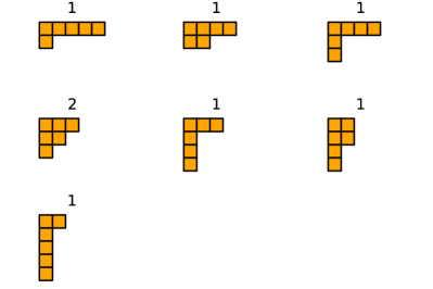
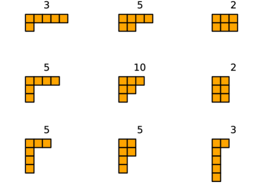
Figure 1: Left: multiplicities of irreducible representations in the tensor product $\rho_{(3,2,1)}\otimes\rho_{(2,2,2)}$ (Clebsch–Gordan coefficients). Right: multiplicities of irreducible representations in the triple tensor product $\rho_{(3,2,1)}\otimes\rho_{(2,2,2)}\otimes\rho_{(3,3)}$.

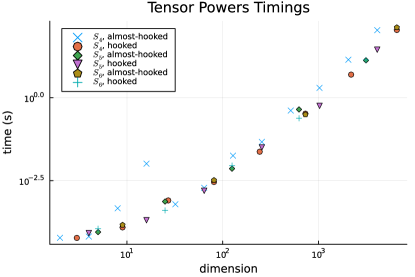
Figure 2: Time taken to compute tensor powers ($\rho^{\otimes k}$) for a hook ($\rho_{(2,1,1,\ldots,1,1)}$) and an almost-hook ($\rho_{(2,2,1,1,\ldots,1,1)}$) irreducible representation for varying $k$ and $n$. We plot the time taken compared to the dimension of the resulting representation to demonstrate the cubic growth in complexity.

For our final example, in Figure 3 we consider the growth in computational cost as $n$ increases for two examples: a hook tensor product $\rho_{(n-1,1)}\otimes\rho_{(2,1,\ldots,1)}$ and an almost-hook tensor product $\rho_{(n-2,1,1)}\otimes\rho_{(2,2,1,\ldots,1)}$ (here the number of ones is taken so that they are both representations of $S_{n}$). The dimensions of the irreducible representations $\rho_{(n-1,1)},\rho_{(n-2,1,1)}$ and $\rho_{(2,1,\ldots,1)}$ are $n-1$, $n+1$ and $n-1$, respectively, so that the tensor products have dimensions $(n-1)^{2}$ and $(n-1)(n+1)$, hence we have demonstrated that the algorithm has polynomial complexity in $n$, in particular at worst ${\mathcal{O}}(n^{7})$ operations. In Figure 3 we plot the time taken showing that the numerical implementation using floating point arithmetic and sparse arrays appears to achieve much better complexity than predicted, in particular we observe ${\mathcal{O}}(n^{2})$ and ${\mathcal{O}}(n^{3})$ complexity. Whether this can be shown rigorously remains open.

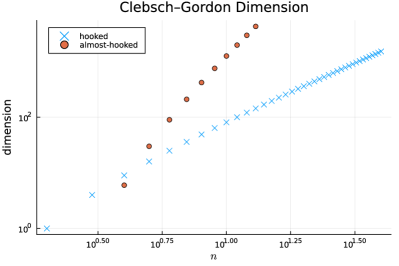
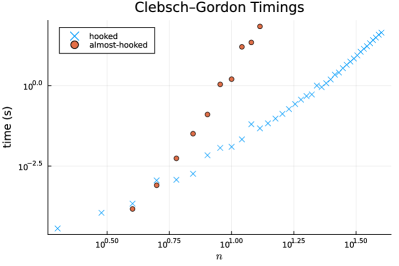
Figure 3: Left: growth in the dimension of a hook ($\rho_{(n-1,1)}\otimes\rho_{(2,1,\ldots,1)}$) and an almost-hook ($\rho_{(n-2,1,1)}\otimes\rho_{(2,2,1,\ldots,1)}$) tensor product. Right: time to compute corresponding Clebsch–Gordan coefficients. This demonstrate polynomial growth with $n$, as a result of the polynomial growth in the dimension.

References

• [1] A. Bunse-Gerstner, R. Byers, and V. Mehrmann. Numerical methods for simultaneous diagonalization. SIAM J. Mat. Anal. Appl., 14(4):927–949, 1993.
• [2] P. Bürgisser and C. Ikenmeyer. The complexity of computing Kronecker coefficients. In Discrete Mathematics and Theoretical Computer Science, pages 357–368. Discrete Mathematics and Theoretical Computer Science, 2008.
• [3] J. D. Dixon. Computing irreducible representations of groups. Maths Comp., 24(111):707–712, 1970.
• [4] W. Fulton and J. Harris. Representation Theory: a First Course, volume 129. Springer Science & Business Media, 2013.
• [5] N. J. Higham. Accuracy and Stability of Numerical Algorithms. SIAM, 2002.
• [6] K. Hymabaccus and D. Pasechnik. Decomposing linear representations of finite groups. arXiv preprint arXiv:2007.02459, 2020.
• [7] K. Hymabaccus and D. Pasechnik. Repndecomp: A gap package for decomposing linear representations of finite groups. Journal of Open Source Software, 5(50):1835, 2020.
• [8] A. Okounkov and A. Vershik. A new approach to representation theory of symmetric groups. Selecta Mathematica New Series, 2(4):581–606, 1996.
• [9] S. Olver. RepresentationTheory.jl v0.0.1, https://github.com/dlfivefifty/RepresentationTheory.jl, 2022.
• [10] I. Pak and G. Panova. On the complexity of computing Kronecker coefficients. Computational Complexity, 26(1):1–36, 2017.
• [11] D. Rosset, F. Montealegre-Mora, and J.-D. Bancal. Replab: A computational/numerical approach to representation theory. In Quantum Theory and Symmetries, pages 643–653. Springer, 2021.
• [12] J.-P. Serre et al. Linear Representations of Finite Groups, volume 42. Springer, 1977.