A new and asymptotically optimally contracting coupling for the random walk Metropolis

Abstract

The reflection-maximal coupling of the random walk Metropolis (RWM) algorithm was recently proposed for use within unbiased MCMC. Numerically, when the target is spherical this coupling has been shown to perform well even in high dimensions. We derive high-dimensional ODE limits for Gaussian targets, which confirm this behaviour in the spherical case. However, we then extend our theory to the elliptical case and find that as the dimension increases the reflection coupling performs increasingly poorly relative to the mixing of the underlying RWM chains. To overcome this obstacle, we introduce gradient common random number (GCRN) couplings, which leverage gradient information. We show that the behaviour of GCRN couplings does not break down with the ellipticity or dimension. Moreover, we show that GCRN couplings are asymptotically optimal for contraction, in a sense which we make precise, and scale in proportion to the mixing of the underling RWM chains. Numerically, we apply GCRN couplings for convergence and bias quantification, and demonstrate that our theoretical findings extend beyond the Gaussian case.

Keywords: Markov chain Monte Carlo methods; Couplings; Optimal scaling; ODE limit

1 Introduction

Couplings of Markov chain Monte Carlo (MCMC) algorithms have attracted much interest recently (jacob2020unbiased; heng2019unbiased; biswas2019estimating; middleton2020unbiased; biswas2021bounding; oleary2021maximal; biswas2021coupling-based; ruiz2021unbiased; nguyen2022many; oleary2022metropolishastings; wang2022unbiasedmultilevel; douc2022solving, etc.) due to their ability to nullify the bias of MCMC estimates (jacob2020unbiased), quantify the convergence of MCMC algorithms (biswas2019estimating), quantify the asymptotic bias of approximate inference procedures (biswas2021bounding).

In the context of unbiased MCMC and the related convergence quantification methodology (jacob2020unbiased; biswas2019estimating), a Markovian coupling of two chains should be designed such that the chains meet after a finite number of iterations. The meeting time acts as a lower bound for the length of the simulation, and as such the efficiency of a coupling can be assessed through the distribution of the meeting time. As remarked in (jacob2020unbiased), it is paramount to design couplings which have favourable high-dimensional properties, in the sense that the meeting times are representative of the true convergence and mixing of the underlying marginal Markov chains. At the same time, it is challenging to design efficient couplings, and this design is regarded to be an art form in general (oleary2022metropolishastings).

Nevertheless, in this paper we address these issues for the random walk Metropolis (RWM) algorithm by introducing gradient common random number (GCRN) couplings, together with an asymptotic framework that certifies their optimality. GCRN couplings scale excellently with the dimension of the target and are insensitive to its ellipticity, being able to consistently contract the chains to within a distance where coalescence in one step is achievable. The GCRN coupling can then be swapped for one which allows for exact meetings; we exemplify and advocate for such a two-scale strategy in the sequel.

The excellent behaviour of the GCRN couplings contrasts with that of status-quo couplings. Arguably the most promising candidate to date, the reflection-maximal coupling (see jacob2020unbiased, Section 4.1), has been seen to scale well with the dimension when the target is spherical or can be preconditioned to be so (jacob2020unbiased; oleary2021maximal; oleary2021couplings). However, when the target is both high-dimensional and elliptical, the reflection-maximal coupling has been seen to perform poorly, as it does not contract the chains sufficiently unless the step size of the coupled RWM algorithms is chosen to be significantly smaller than optimal (papp2022paper). The present work also offers an explanation of the failings of the reflection coupling for elliptical targets, which was the original motivation for our analysis.

Our analysis reconciles coupled MCMC sampling with the MCMC dimensional scaling literature (see e.g. roberts1997weak; roberts1998optimal; roberts2001optimal; sherlock2009optimal; beskos2013optimal; sherlock2013optimal for the stationarity phase, and christensen2005scaling for the transient phase). The ODE limit in christensen2005scaling for high-dimensional spherical Gaussian targets, originally developed to explain the transient phase of the RWM algorithm, underpins our approach. We extend this limit to coupled pairs of RWM chains in the spherical Gaussian case, and further extend the salient points of this analysis to the elliptical Gaussian case. In addition to revealing that the GCRN coupling is asymptotically optimal in terms of contraction, another takeaway from our analysis is that gradient information is necessary for a coupling of the RWM to perform well for high-dimensional elliptical targets. However, once gradient information is incorporated into the coupling, our analysis and supporting numerical experiments on both Gaussian and non-Gaussian targets demonstrate that the convergence of the RWM algorithm can be accurately and robustly estimated even in high dimension.

1.1 Overview of the paper

Our paper is organized as follows. In Section 2 we argue for the importance of contractive couplings in high-dimensional settings. We then introduce the GCRN coupling, alongside the other two couplings under our consideration, the CRN and reflection couplings.

In Section 3 we analyze the couplings under the assumption that the target is a high-dimensional standard Gaussian. Theorem 1, our main result, establishes high-dimensional ODE limits which explain the behaviour of each coupling. Proposition 3 describes the fixed points of the ODE limits, from which we infer the long-time behaviour of the coupled chains. The GCRN and reflection couplings perform satisfactorily here. Theorem 2 establishes that the GCRN coupling is asymptotically optimal for contraction among a class of couplings which are amenable to implementation. Finally, we discuss the step size scaling of the three couplings, which we find is favourable under GCRN and reflection.

In Section 4, we assume that the target is elliptical Gaussian. Extending much of the analysis of Section 3, we derive the long-time behaviour of the chains under each coupling (Theorem 3). As opposed to the spherical case, in the elliptical case we find that only the GCRN coupling contracts the chains satisfatorily. We again establish that the GCRN coupling is asymptotically optimal for contraction (Theorem 4) and scales favourably with the step size.

In Section 5 we demonstrate some applications of the GCRN coupling, in a high-dimensional non-Gaussian setting. Firstly, we use the GCRN coupling, combined with the reflection-maximal coupling in a two-scale fashion, to estimate the convergence of the RWM algorithm. Secondly, we estimate the bias of an approximate inference procedure with the GCRN coupling. Finally, we extend the GCRN coupling to a variant of the RWM with a position-dependent covariance. We then use this coupling to estimate the convergence of a recently-proposed gradient-based algorithm.

In Section 6 we conclude and offer directions for future research. The proofs of the main results are provided in Appendix A. All other appendices contain supporting information. Code to reproduce the numerical experiments can be found at https://github.com/tamaspapp/rwmcouplings.

1.2 Notation

The standard normal probability and cumulative density functions are denoted by $\phi$ and $\Phi$, respectively. The bivariate normal distribution with unit coordinate-wise variances and correlation $\rho\in[-1,1]$ is denoted by $\operatorname{BvN}(\rho)$. The Euclidean norm is denoted by $\lVert\cdot\rVert$. For any positive definite matrix $A$, we define the inner product $\langle x,y\rangle_{A}=x^{\top}Ay$ and the squared norm $\lVert x\rVert_{A}^{2}=x^{\top}Ax$. We employ the standard Bachmann-Landau asymptotic notation $O,o$ and $\Theta$, we also use subscripting as in $\Theta_{d}$ when making the dependence on the dimension $d$ explicit.

2 Couplings of the RWM algorithm

We consider two coupled chains $(X,Y)=\{(X_{t},Y_{t})\}_{t\geq 0}$ evolving according to the one-step random walk Metropolis (RWM) updates

$$X_{t+1}=X_{t}+hZ_{x}B_{x},\quad Y_{t+1}=Y_{t}+hZ_{y}B_{y},$$ (1)

where $B_{x}=\mathbbm{1}\{U_{x}\leq A(X_{t},Z_{x})\}$ is the Bernoulli acceptance indicator, and $A(X_{t},Z_{x})=\pi(X_{t}+hZ_{x})/\pi(X_{t})$ is the Metropolis acceptance ratio for the $X$-chain. Here, $Z_{x}\sim\mathcal{N}_{d}(0,I_{d})$ and $U_{x}\sim\textup{Unif}(0,1)$ are independent. Analogous notation applies to the $Y$-chain.

The couplings we consider are Markovian: at each step we couple $(U_{x}\otimes Z_{x},U_{y}\otimes Z_{y})$ conditionally on $(X_{t},Y_{t})$, where $\otimes$ denotes independence between random variables, and it holds that the joint process $(X,Y)=\{(X_{t},Y_{t})\}_{t\geq 0}$ is itself a Markov chain. We furthermore restrict our attention to the class of couplings $\mathcal{I}$ which we deem amenable to implementation, see Definition 1 below.

Definition 1 (Class of product couplings).

The class $\mathcal{I}$ of “product” couplings of the RWM kernels (1) is the set of all couplings where the coupled acceptance uniforms $(U_{x},U_{y})$ are independent of the coupled proposal increments $(Z_{x},Z_{y})$.

The class of Markovian couplings for the RWM is strictly larger than $\mathcal{I}$: it is possible to implement couplings which, say, correlate $U_{x}$ and $Z_{y}$. Examples include the maximal transition kernel couplings considered in (oleary2021maximal; oleary2022metropolishastings). We however demonstrate that, in terms of contraction in the $d\to\infty$ asymptotic regime, the best Markovian coupling can only offer a minor improvement over the best coupling in $\mathcal{I}$, see Remark 4.

2.1 The importance of contractivity in high dimension

It is possible to design couplings of (1) which have a positive (and even maximal) chance of coalescing the chains at each iteration, see (oleary2021maximal). While such couplings have been seen to be effective in low dimensions, in high dimensions their performance can be severely hampered by the typically large distances between chains, as Remark 1 below shows.

Remark 1.

For any Markovian coupling of the RWM updates (1), the probability of coalescing the chains in one iteration is upper bounded by the overlap of the proposal densities $p=\mathbb{P}\{|\mathcal{N}(0,1)|\geq\lVert X_{t}-Y_{t}\rVert/(2h)\}$ (e.g. heng2019unbiased, Section 4.1). Under the scaling $h=ld^{-1/2}$ which ensures that acceptance probabilities remain $\Theta(1)$ as the dimension $d\to\infty$ (roberts1997weak), it holds that $p\leq 2\exp(-l^{2}\lVert X_{t}-Y_{t}\rVert^{2}d/8)$ by the usual Gaussian tail bound. Two independent chains will typically start $\lVert X_{0}-Y_{0}\rVert^{2}=\Theta(d)$ apart in high dimension; if the coupling cannot contract the chains to within $\lVert X_{t}-Y_{t}\rVert^{2}=O(1)$, the chance of coalescing the chains in one iteration decays (at least) exponentially in the dimension $d$.

As such, if the coupling does not enable the chains to contract to within $O(1)$, one can expect the average meeting time to grow (at least) exponentially with the dimension $d$. Furthermore, for practical purposes, the chance of coalescing the chains in one iteration is infinitesimally small in high dimension $d$ unless $\lVert X_{t}-Y_{t}\rVert^{2}=O(1/d)$, so the chains cannot meet unless they first contract to within such a distance.

In high dimensions, a coupling should therefore be primarily focused on contracting the coupled chains, as opposed to maximizing the probability of meeting at each iteration, as has also been noted in (oleary2021maximal). As such, in this paper our focus is on couplings which bring the chains (extremely) close together in squared distance $\lVert X_{t}-Y_{t}\rVert^{2}$ as $t$ increases. A natural quantity to optimize is therefore the one-step difference $\lVert X_{t+1}-Y_{t+1}\rVert^{2}-\lVert X_{t}-Y_{t}\rVert^{2}$, which can be interpreted as the absolute contraction of the chains over one step, and which we can expand as

$$\underbrace{\lVert X_{t+1}\rVert^{2}-\lVert X_{t}\rVert^{2}}_{(i)}+\underbrace{\lVert Y_{t+1}\rVert^{2}-\lVert Y_{t}\rVert^{2}}_{(ii)}-2\underbrace{(X_{t+1}^{\top}Y_{t+1}-X_{t}^{\top}Y_{t})}_{(iii)}.$$ (2)

We further expand the term $(iii)$,

$$X_{t+1}^{\top}Y_{t+1}-X_{t}^{\top}Y_{t}= hY_{t}^{\top}Z_{x}B_{x} +$$ (3)

$$hX_{t}^{\top}Z_{y}B_{y} +$$ (4)

$$h^{2}Z_{x}^{\top}Z_{y}B_{x}B_{y}.$$ (5)

Conditional on $X_{t}$ and $Y_{t}$, the distributions of the terms $\{(i),(ii),\eqref{eqn:innerprod-x},\eqref{eqn:innerprod-y}\}$ are invariant to the coupling used. If the objective is to minimize $\mathbb{E}[\lVert X_{t+1}-Y_{t+1}\rVert^{2}-\lVert X_{t}-Y_{t}\rVert^{2}\mid X_{t},Y_{t}]$, that is (on average) to contract the chains as much as possible over one step, it is therefore solely term (5) which determines the efficiency of the coupling.

We shall use this observation in Sections 3.5 and 4.3 in order to define objectives which quantify the contraction of the chains in high dimension. However, from the form of (5) one can already devise a strategy which optimizes the expected contraction: correlate the acceptances $B_{x},B_{y}$ maximally (i.e. try to accept simultaneously) and correlate the proposal noises $Z_{x},Z_{y}$ maximally. While it is infeasible to do both in low dimension, as the dimension increases the two objectives become less and less constrained by each other. Therefore, when the dimension is high, both objectives can at least approximately be satisfied. By Taylor expanding the log-acceptance ratio $\log A(X_{t},Z_{x})$, it becomes clear that in high dimension the acceptance probability is essentially a deterministic function of the projection of $Z_{x}$ onto the gradient at $X_{t}$. To correlate $B_{x},B_{y}$ maximally, it is therefore sensible to maximally correlate the projections of $Z_{x},Z_{y}$ onto the respective gradients at $X_{t}$ and $Y_{t}$. This only constrains one coordinate of each of $Z_{x}$ and $Z_{y}$, and so in high dimension $Z_{x}$ and $Z_{y}$ can still be correlated nearly maximally. This is the motivation behind the gradient-based GCRN coupling which we introduce in Section 2.2.

2.2 Couplings under consideration

We focus our attention on three couplings. The first two are established, having for example been considered in the simulation study (oleary2021couplings): the common random number (CRN) coupling and the reflection coupling. The third is the gradient common random number (GCRN) coupling, which we introduce. All three couplings couple the uniform acceptance random variables synchronously (i.e. by common random numbers): $U_{y}=U_{x}$. They differ, however, in the way they couple the proposal increments $Z_{x},Z_{y}$:

• CRN: $Z_{y}=Z_{x}$.

• Reflection: $Z_{y}=Z_{x}-2(e^{\top}Z_{x})e$, where $e=(X_{t}-Y_{t})/\lVert X_{t}-Y_{t}\rVert$.

• GCRN: $Z_{x}=Z-(n_{x}^{\top}Z)n_{x}+Z_{1}n_{x}$ and $Z_{y}=Z-(n_{y}^{\top}Z)n_{y}+Z_{1}n_{y}$, where $n_{x},n_{y}$ are the normalized gradients at $X_{t},Y_{t}$ respectively, and $Z_{1}\sim\mathcal{N}(0,1)$ and $Z\sim\mathcal{N}_{d}(0,I_{d})$ are independent.

While none of the three couplings allows for the chains to meet, one can for instance swap to a coupling that allows for exact meetings once the chains are close enough to have a reasonable chance of coalescing in one step. We shall consider such a two-scale approach for the GCRN coupling in Section 5.1.

The GCRN coupling is so named because the projections of the noises $Z_{x},Z_{y}$ in the directions of the gradients are identical ($n_{x}^{\top}Z_{x}=n_{y}^{\top}Z_{y}$) and hence we use “common random numbers in the direction of the gradients”. Furthermore, when $d\geq 2$, the $d-2$ coordinates orthogonal to the span of the gradients use common random numbers.

Remark 2 (Other GCRN variants).

The couplings $Z_{y}=R(n_{x},n_{y})Z_{x}$, where $R(n_{x},n_{y})$ is either the linear map $(i)$ rotating $n_{x}$ to $n_{y}$ in $\textup{span}\{n_{x},n_{y}\}$ while leaving the complement space unchanged, or $(ii)$ reflecting in $\tilde{e}=n_{x}-n_{y}$, can be considered variants of the GCRN coupling in that $n_{x}^{\top}Z_{x}=n_{y}^{\top}Z_{y}$ and $\lim_{d\to\infty}Z_{x}^{\top}Z_{y}/d=1$, where the convergence is in $L_{2}$. These couplings enjoy similar high-dimensional properties to the GCRN coupling.

In our subsequent analysis, a recurrent quantity is the correlation (equivalently, the covariance) of the projections $n_{x}^{\top}Z_{x}$ and $n_{y}^{\top}Z_{y}$. We evaluate this for each coupling in Proposition 1 below. As with all our results, this is proved in Appendix A.

Proposition 1 (Correlation of projections onto gradients).

For each of the three couplings, the value of $\rho=\textup{Corr}(n_{x}^{\top}Z_{x},n_{y}^{\top}Z_{y})=\textup{Cov}(n_{x}^{\top}Z_{x},n_{y}^{\top}Z_{y})$ is, respectively

$$\rho_{\textup{crn}}=n_{x}^{\top}n_{y},\quad\rho_{\textup{refl}}=n_{x}^{\top}n_{y}-2(n_{x}^{\top}e)(n_{y}^{\top}e),\quad\rho_{\textup{gcrn}}=1.$$

3 Standard Gaussian case

Here we consider a standard Gaussian target $\pi=\mathcal{N}_{d}(0,I_{d})$. Our analysis relies heavily on the form of the RWM acceptance ratio in the standard Gaussian case, $A(X_{t},Z_{x})=\exp(-hX_{t}^{\top}Z_{x}-h^{2}\lVert Z_{x}\rVert^{2}/2)$.

(christensen2005scaling) argue that the process $(\lVert X_{\lfloor td\rfloor}\rVert^{2}/d)_{t\geq 0}$ is the natural one to consider when investigating the transient phase of the RWM algorithm targeting $\mathcal{N}_{d}(0,I_{d})$. Indeed, due to the spherical symmetry of the target, the process is Markov and enables explicit calculations which lead to a precise quantification of its asymptotic behaviour. Time is sped up by a factor of $d$, as this is the natural timescale under a step size $h\sim d^{-1/2}$.

By extension, inspecting the terms in the expansion (2), the three-dimensional process

$$W^{(d)}=(W^{(d)}_{t})_{t\geq 0}=\frac{1}{d}\left(\lVert X_{\lfloor td\rfloor}\rVert^{2},\lVert Y_{\lfloor td\rfloor}\rVert^{2},X_{\lfloor td\rfloor}^{\top}Y_{\lfloor td\rfloor}\right)_{t\geq 0}$$

is the natural one to consider for a pair of RWM chains evolving jointly with step size $h\sim d^{-1/2}$. Intuitively, in the high-dimensional setting, the re-scaled squared norms act as radial terms quantifying the distance of the chains from the approximately spherical main mass (e.g. the $X$-chain is in the main mass when $\lVert X_{t}\rVert^{2}/d\approx 1$). Conditional on these two radial components and normalized by $\lVert X_{t}\rVert\lVert Y_{t}\rVert/d$, the inner product corresponds to the cosine of the angle between $X_{t}$ and $Y_{t}$.

This process is Markov under our couplings of interest (see Appendix H for a proof sketch). This enables us to derive ODE limits which extend those of (christensen2005scaling) and which explain the behaviour of the coupled Markov chains in the high-dimensional case.

3.1 Preliminary calculations

In this section, we perform explicit calculations which shall aid in deriving the ODE limit of the process $W^{(d)}$. For all $X,Y>0$, we define the set

$$\mathcal{S}(X,Y)=\{(x,y,v)\mid x\in[0,X],y\in[0,Y],|v|\leq\sqrt{xy}\}.$$

Note that $\mathcal{S}=\bigcup_{X,Y>0}\mathcal{S}(X,Y)$ contains all feasible values for the process $W^{(d)}$.

3.1.1 The coupling-invariant terms

Expanding the acceptance ratio, we have that

$$\eqref{eqn:innerprod-x}=hY_{t}^{\top}Z_{x}\mathbbm{1}\big{\{}U_{x}\leq\exp(-hX_{t}^{\top}Z_{x}-h^{2}\lVert Z_{x}\rVert^{2}/2)\big{\}}.$$

Conditioning on $W^{(d)}_{t/d}=(x,y,v)$, and in the limit as $d~{}\to~{}\infty$, the above term has an expectation that is well-defined as a function of $(x,y,v)$.

Lemma 1 (Limit of coupling-invariant terms).

Let $h=ld^{-1/2}$. Conditional on $W^{(d)}_{t/d}=(x,y,v)$, it holds that

$$\lim_{d\to\infty}\mathbb{E}\eqref{eqn:innerprod-x} =-vl^{2}e^{l^{2}(x-1)/2}\Phi(l/(2x^{1/2})-lx^{1/2}),$$

$$\lim_{d\to\infty}\mathbb{E}\eqref{eqn:innerprod-y} =-vl^{2}e^{l^{2}(y-1)/2}\Phi(l/(2y^{1/2})-ly^{1/2}).$$

Moreover, both convergences are uniform over all $(x,y,v)\in\mathcal{S}(X,Y)$, whatever fixed $X,Y>0$.

At $x=1$, heuristically corresponding to a high-dimensional chain evolving at stationarity, the first limit in Lemma 1 simplifies to $-vl^{2}\Phi(-l/2)$. This is proportional (by a factor $-v/2$) to the Expected Squared Jumping Distance (ESJD; e.g. sherlock2009optimal) of a RWM chain at stationarity.

The ESJD is a measure of efficiency for the mixing of the RWM algorithm. According to well-known asymptotic analyses considering the optimal scaling of the RWM at stationarity (roberts1997weak), optimizing the ESJD returns the optimal scaling $l=2.38$ and optimal acceptance rate of $23.4\%$. As in such analyses, the ESJD shall play a key part in our discussion of the optimal scaling of coupled RWM algorithms (see Section 3.6).

3.1.2 The coupling-dependent term

While terms (3) and (4) are independent of the coupling, term (5) does depend on the coupling used. In the proposition below we derive the asymptotic expectation of this term conditional on $W^{(d)}_{t/d}=(x,y,v)$, for the three couplings under consideration.

Lemma 2 (Limit of coupling-dependent term).

Let $h=ld^{-1/2}$ and assume that one of the CRN, reflection, or GCRN couplings is used. Conditional on $W^{(d)}_{t/d}=(x,y,v)$, it holds that

$$\lim_{d\to\infty}\mathbb{E}\eqref{eqn:innerprod-cross}=l^{2}g(x,y,v),$$

where

$$g(x,y,v)=\mathbb{E}_{(Z_{1},Z_{2})\sim\operatorname{BvN}(\rho)}\left\{1\land e^{-lx^{1/2}Z_{1}-l^{2}/2}\land e^{-ly^{1/2}Z_{2}-l^{2}/2}\right\}$$

and $\rho=\rho(x,y,v)$ is

$$\rho_{\textup{crn}}=\frac{v}{(xy)^{1/2}},\quad\rho_{\textup{refl}}=\frac{2xy-(x+y)v}{(xy)^{1/2}(x+y-2v)},\quad\rho_{\textup{gcrn}}=1.$$

Moreover, all convergences are uniform over all $(x,y,v)\in\mathcal{S}(X,Y)$, whatever $X,Y>0$.

See Appendix D for the computation of $g$ under arbitrary correlation. For the GCRN coupling, this quantity is tractable (see Lemma 6 in Appendix B); letting $m=x\land y$ and $M=x\lor y$, we have

$$g_{\textup{gcrn}}(x,y,v)=\Phi(-\frac{l}{2m^{1/2}})+e^{l^{2}(m-1)/2}\left\{\Phi(\frac{l}{2m^{1/2}}-lm^{1/2})-\Phi(-lm^{1/2})\right\}+e^{l^{2}(M-1)/2}\Phi(-lM^{1/2}).$$

When $x=y=1$, which heuristically corresponds to both chains being marginally stationary in high dimension, it holds that $l^{2}g_{\textup{gcrn}}(x,y,v)=2l^{2}\Phi(-l/2)$ for all $z$. This is the ESJD of a RWM chain at stationarity — we offer the following explanation for this apparent coincidence. When both chains are marginally stationary, under the GCRN coupling both chains essentially accept and reject at the same time, and both proposal increments are in approximately the same direction because they share all but two of the $d$ coordinates (the GCRN coupling was designed with precisely this behaviour in mind). As such, $\eqref{eqn:innerprod-cross}\approx l^{2}(\lVert Z_{x}\rVert^{2}/d)B_{x}$, and in the limit $d\to\infty$ the latter term is precisely the ESJD.

Remark 3 (Similarity between GCRN and reflection coupling at stationarity).

As far as contraction in the $d\to\infty$ limit is concerned, the reflection and GCRN couplings are equivalent when both of the marginal RWM chains are stationary. This is since, by Lemma 2, when $x=y=1$ it holds that $\rho_{\textup{gcrn}}=\rho_{\textup{refl}}=1$ irrespective of $v\in[-1,1]$. The GCRN coupling is, in fact, asymptotically optimal among all couplings amenable to practical implementation (Section 3.5) and enjoys favourable dimensional scaling (Section 3.6). The good performance of the reflection coupling in the spherical case can thus be explained through its similarities with the GCRN coupling. However, note that the reflection coupling loses efficiency compared to the GCRN coupling when either of the marginal chains is in its transient phase.

3.2 ODE limits for coupled RWM chains

With the preliminary calculations in hand, we are in a position to apply the argument of (christensen2005scaling) and show that $W^{(d)}$ converges weakly to the solution of an ordinary differential equation as $d\to\infty$.

The first part of the argument is the uniform convergence of the infinitesimals of $W^{(d)}$. christensen2005scaling deals with the first two components of $W^{(d)}_{(t+1)/d}-W^{(d)}_{t/d}$. The third component of this quantity is $X_{t+1}^{\top}Y_{t+1}-X_{t}^{\top}Y_{t}=\eqref{eqn:innerprod-x}+\eqref{eqn:innerprod-y}+\eqref{eqn:innerprod-cross}$, which is dealt with by Lemmas 1 and 2. Therefore, we have the following:

Corollary 1 (Convergence of the infinitesimals of the discrete process).

Let $h=ld^{-1/2}$, and let the coupling be either CRN, reflection, or GCRN. It holds that

$$\lim_{d\to\infty}\mathbb{E}\left\{W^{(d)}_{(t+1)/d}-W^{(d)}_{t/d}\mid W^{(d)}_{t/d}=w\right\}d=c(w),$$

where for all $w=(x,y,v)^{\top}\in\mathcal{S}(X,Y)$ we have $c(w)=l^{2}\big{(}a(x),a(y),b(x,y,z)\big{)}^{\top}$, with

$$a(x)= (1-2x)e^{l^{2}(x-1)/2}\Phi(\frac{l}{2x^{1/2}}-lx^{1/2})+\Phi(-\frac{l}{2x^{1/2}}),$$

$$b(x,y,v)= g(x,y,v)-v\left\{e^{l^{2}(x-1)/2}\Phi(\frac{l}{2x^{1/2}}-lx^{1/2})+e^{l^{2}(y-1)/2}\Phi(\frac{l}{2y^{1/2}}-ly^{1/2})\right\},$$

and $g$ is as in Lemma 2 and depends on the particular coupling.

Moreover, the convergence is uniform over all $w\in\mathcal{S}(X,Y)$, whatever $X,Y>0$.

In addition to the above result, we also require the following uniform bound for our subsequent ODE limits. As for Corollary 1, the contribution from the first two components is due to christensen2005scaling.

Proposition 2 (Uniform bound on fluctuations).

Let $h=ld^{-1/2}$ and let the coupling be CRN, reflection or GCRN. For all $X,Y>0$, it holds that

$$\lim_{d\to\infty}\sup_{w\in\mathcal{S}(X,Y)}\mathbb{E}\left\{\lVert W^{(d)}_{(t+1)/d}-W^{(d)}_{t/d}\rVert^{2}\mid W^{(d)}_{t/d}=w\right\}d^{2}<\infty.$$

Finally, by using Corollary 1 and Proposition 2, we arrive at our main result: ODE limits, as $d\to\infty$, for the process $W^{(d)}=(W^{(d)}_{t})_{t\geq 0}$ under each of the three couplings.

Theorem 1 (ODE limits for coupled RWM).

Let $h=ld^{-1/2}$ and $W^{(d)}_{0}=w_{0}\in\mathcal{S}$ for all $d$. Let the function $c$ be as defined in Corollary 1, where the coupling used can be CRN, reflection or GCRN. Then, $W^{(d)}\implies w=(x,y,v)$ as $d\to\infty$, where $w:[0,\infty)\to\mathcal{S}$ is the solution of the initial value problem

$$\dot{w}(t)=c(w(t))\quad\textup{started from }w(0)=w_{0}.$$ (IP)

Our interest lies in the squared distance $\lVert X_{t}-Y_{t}\rVert^{2}$. Replacing the inner product process in third coordinate of $W^{(d)}$ with the squared-distance process, we define

$$F^{(d)}=(F^{(d)}_{t})_{t\geq 0}=\frac{1}{d}\left(\lVert X_{\lfloor td\rfloor}\rVert^{2},\lVert Y_{\lfloor td\rfloor}\rVert^{2},\lVert X_{\lfloor td\rfloor}-Y_{\lfloor td\rfloor}\rVert^{2}\right)_{t\geq 0}.$$

As a corollary of Theorem 1 we obtain the ODE limit $F^{(d)}\implies f=(x,y,s)$ as $d\to\infty$, where $f$ solves

$$\dot{f}(t)=e(f(t)),\quad\textup{with }e(x,y,s)=l^{2}\big{(}a(x),a(y),d(x,y,s)\big{)}^{\top}$$ (SD)

and $e(x,y,s)=a(x)+a(y)-2b\big{(}x,y,(x+y-s)/2\big{)}$. We have obtained the ODE (SD) for the squared distance from the ODE (IP) for the inner product by the change of variables $s=x+y-2v$.

3.3 Numerical illustration

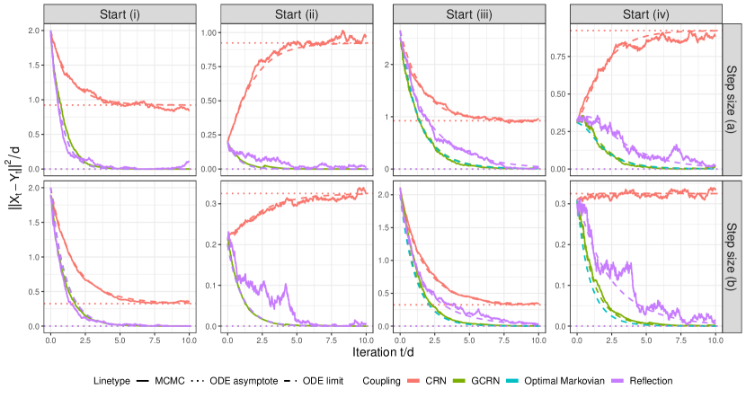
Figure 1: (Spherical case.) MCMC trace of $\lVert X_{t}-Y_{t}\rVert^{2}/d$ against $t/d$, and ODE limit (SD) for the rescaled and sped up squared distance between chains, computed for all three couplings as described in Section 3.3. The stable fixed points of the ODEs (see Section 3.4) appear as dotted horizontal lines. Additionally, the ODE limit for the asymptotically optimal Markovian coupling (see Remark 4 in Section 3.5) appears as a dashed blue line.

We illustrate the ODE limit (SD) through four different starting conditions $(x_{0},y_{0},v_{0})$, where $v_{0}=\rho_{0}(x_{0}y_{0})^{1/2}$ and here $\rho_{0}$ corresponds to the correlation between the starting values of the chains. These are, and heuristically correspond to chains started from:

1. $(x_{0},y_{0},\rho_{0})=(1,1,0)$, independent draws from the target.

2. $(x_{0},y_{0},\rho_{0})=(1,1,0.9)$, positively correlated draws from the target.

3. $(x_{0},y_{0},\rho_{0})=(1.5,0.5,0)$, independent draws from, respectively, over- and under-dispersed versions of the target.

4. $(x_{0},y_{0},\rho_{0})=(0.4,0.01,-0.5)$, negatively correlated draws, from under-dispersed versions of the target.

We use step sizes $(a)$ $l=2.38$ and $(b)$ $l=\sqrt{2}$. The former is the stationary-optimal scaling of the RWM algorithm in high dimension (roberts1997weak), and both step sizes are close to optimal for the transient phase (christensen2005scaling). For the coupled MCMC samplers, we fix the dimension to $d=1000$ and sample the initial conditions $(X_{0}^{d},Y_{0}^{d})$ according to $X_{0}^{d}=x_{0}^{1/2}Z$ and $X_{0}^{d}=y_{0}^{1/2}\{\rho_{0}Z+(1-\rho_{0}^{2})^{1/2}Z_{*}\}$, where $Z,Z_{*}\sim\mathcal{N}_{d}(0,I_{d})$ independently.

As per Figure 1, the squared distance between the chains closely follows the limiting ODE trajectory under each coupling. Moreover, the distance asymptotes at the stable fixed point that will be predicted by the theory of Section 3.4. Stochasticity is clearly present in the MCMC traces, however this is a consequence of $d<\infty$ and the noise vanishes in the limit as $d\to\infty$. For all starting conditions, the GCRN coupling is clearly the best performer among the three implementable couplings.

In addition to the ODE limits for the GCRN, CRN and reflection couplings, we have computed the ODE limit for the asymptotically optimal Markovian coupling (this is tractable, see Appendix C). Figure 1 reveals that the GCRN coupling closely approximates the asymptotically optimal Markovian coupling.

3.4 Long-time limit of the distance between the chains

In this section, we derive the behaviour the squared distance $\lVert X_{t}-Y_{t}\rVert^{2}$ in the joint long-time and high-dimensional limits.

For any fixed $d$, the process $\{(X_{t},Y_{t})\}_{t\geq 0}$ is Markov and ergodic, and so its distribution stabilizes as $t\to\infty$. In view of the ODE limit $F^{(d)}\implies f$, one might therefore expect $\lim_{t\to\infty}f(t)$ to be unique. At least informally, the third coordinate of this limit provides the limiting squared distance $s_{\infty}=\lim_{d,t\to\infty}\lVert X_{t}-Y_{t}\rVert^{2}/d$. We shall access $\lim_{t\to\infty}f(t)$ through the stable fixed points of the ODE (SD). For simplicity, in Proposition 3 below we characterize the fixed points of the ODE (IP). The fixed points of the ODE (SD) follow by a change of variables.

Before stating Proposition 3, let us remark on the form of the ODE (IP). Its first two coordinates are autonomous equations, which simplifies the stability analysis considerably: one only needs to check the sign of the diagonal entries of the Jacobian of $c$. Since $\lim_{d\to\infty}\lim_{t\to\infty}\lVert X_{t}\rVert^{2}/d=\lim_{d\to\infty}\lim_{t\to\infty}\lVert Y_{t}\rVert^{2}/d=1$ in $L_{2}$, the unique stable fixed points in the first two coordinates must therefore be $x=y=1$. This corresponds to both chains being, marginally, stationary.

Proposition 3 (Fixed points of limiting ODE (IP)).

Consider the limiting ODE (IP). The unique fixed point for the autonomous first two coordinates is $(x,y)=(1,1)$ and is stable. The fixed points in the third coordinate are:

• GCRN and reflection couplings: $v_{\textup{gcrn}}=v_{\textup{refl}}=1$ (stable).

• CRN coupling: $v_{\textup{crn}}\in(0,1)$ (stable) and $v_{u}=1$ (unstable).

The value $v_{\textup{crn}}$ is the unique solution of $h(v)-vl^{2}\Phi(-l/2)=0$ which lies inside $v\in(0,1)$, where $h(v)=\mathbb{E}_{(Z_{1},Z_{2})\sim\operatorname{BvN}(v)}(1\land e^{-lZ_{1}-l^{2}/2}\land e^{-lZ_{2}-l^{2}/2})$. Moreover, $v_{\textup{crn}}$ is decreasing in $l$ and $\lim_{l\to 0}v_{\textup{crn}}=1$, $\lim_{l\to\infty}v_{\textup{crn}}=0$.

Proposition 3 indicates that (IP) has a unique stable fixed point under each coupling. As argued above, this stable fixed point dictates the behaviour of $\lVert X_{t}-Y_{t}\rVert^{2}/d$ for large $d$ and $t$, at least from a non-trivial initial condition $X_{0}\neq Y_{0}$. As $t\to\infty$ and for large $d$, $\lVert X_{t}-Y_{t}\rVert^{2}/d\approx x+y-2v=2(1-v)=:s_{\infty}$, where $v$ is the stable point as defined in Proposition 3.

For the GCRN and reflection couplings, $s_{\infty}=0$, and so these couplings contract the chains satisfactorily even in high dimensions. For the CRN coupling it holds that $s_{\infty}>0$, which is problematic in high dimensions. The quantities $v_{\textup{crn}}$ and $s_{\infty}$ under the CRN coupling are graphed against $l$ in Figure 2. We remark on the consequences for the dimensional scaling of the three couplings in more detail in Section 3.6.

Figure 2: (Spherical case.) Asymptotes $v_{\textup{crn}}$ for $X_{t}^{\top}Y_{t}/d$ (left) and $s_{\infty}$ for $\lVert X_{t}-Y_{t}\rVert^{2}/d$ (right) under the CRN coupling, against the step size parameter $l$. The ESJD of each of the marginal chains, as a function of $l$, is overlaid as a dashed line for additional context.

3.5 Asymptotic optimality

In this section we propose an asymptotic framework in which to assess the effectiveness of the couplings under our consideration. The framework and the main result of this section do not rely on the ODE limits (IP) and (SD), although they are related to them.

If we wish to contract the chains as quickly as possible, it is sensible to minimize the expected difference $\mathbb{E}\{\lVert X_{t+1}-Y_{t+1}\rVert^{2}-\lVert X_{t}-Y_{t}\rVert^{2}\mid X_{t},Y_{t}\},$ over some set of couplings of RWM kernels. Following the expansion (2) in Section 2, it is equivalent to maximize $\mathbb{E}\{\eqref{eqn:innerprod-cross}\mid X_{t},Y_{t}\}$, which equals $\mathbb{E}\{\eqref{eqn:innerprod-cross}\mid\lVert X_{t}\rVert^{2},\lVert Y_{t}\rVert^{2},X_{t}^{\top}Y_{t}\}$ for the CRN, reflection and GCRN couplings. We are interested in the high-dimensional asymptotic regime, which requires quantities to be appropriately re-scaled. Therefore, we settle with maximizing, in the limit as $d\to\infty$, the objective

$$\mathbb{E}\left[\eqref{eqn:innerprod-cross}\mid\frac{\lVert X_{t}\rVert^{2}}{d}=x,\frac{\lVert Y_{t}\rVert^{2}}{d}=y,\frac{X_{t}^{\top}Y_{t}}{d}=v\right]$$ (6)

over $(x,y,v)\in\mathcal{S}$.

We shall seek to maximize the objective (6) over the class $\mathcal{I}$ (see Definition 1) of Markovian couplings which are amenable to practical implementation. The main result of this section is that the GCRN coupling is uniformly optimal for contraction among all couplings in $\mathcal{I}$.

Theorem 2 (Optimality of GCRN coupling).

Let $\widetilde{K}$ be the coupling of the RWM kernels $(K(X_{t},\cdot),K(Y_{t},\cdot))$ of equation (1) with step size $h=ld^{-1/2}$. Then, for all $(x,y,v)\in\mathcal{S}$,

$$\lim_{d\to\infty}\sup_{\widetilde{K}\in\mathcal{I}}\mathbb{E}\left[\eqref{eqn:innerprod-cross}\mid\frac{\lVert X_{t}\rVert^{2}}{d}=x,\frac{\lVert Y_{t}\rVert^{2}}{d}=y,\frac{X_{t}^{\top}Y_{t}}{d}=v\right]=l^{2}\mathbb{E}\left[1\land e^{-lx^{1/2}Z-l^{2}/2}\land e^{-ly^{1/2}Z-l^{2}/2}\right],$$

where $Z\sim\mathcal{N}(0,1)$, and the right-hand side is attained by the GCRN coupling.

Suppose that one uses a coupling which give rises to an ODE limit as in Theorem 1. The process $S_{t}^{(d)}=\lVert X_{\lfloor td\rfloor}-Y_{\lfloor td\rfloor}\rVert^{2}/d$ therefore also has a deterministic limit $S(t)$ as $d\to\infty$, given by the third coordinate of (SD). Optimizing (6) means optimizing the drift of $S(t)$ towards its limiting value $s_{\infty}=\lim_{t\to\infty}S(t)$.

Remark 4 (Asymptotically optimal Markovian coupling).

Suppose that the objective is to maximize (6) over the class of all Markovian couplings $\mathcal{M}\supset\mathcal{I}$, and in the limit as $d\to\infty$. We construct an asymptotically optimal Markovian coupling in Appendix C; the slight improvement in convergence over the GCRN coupling is shown in Figure 1.

3.6 Dimensional scaling

In Section 3.5, we fixed the step size $h=ld^{-1/2}$, the correct scaling for both the stationary and transient phases of the RWM algorithm (roberts1997weak; christensen2005scaling), and showed that the GCRN coupling is optimal for contraction among all couplings in $\mathcal{I}$, the class of couplings amenable to practical implementation. In this section, we instead fix the coupling and investigate the optimal scaling of the step size $h=ld^{-1/2}$ with the view of optimizing the contraction of the chains.

By Remark 1, the primary objective is to bring the chains vanishingly close as $t\to\infty$, that is $s_{\infty}=0$. Under the CRN coupling, when $l=\Theta_{d}(1)$ it holds that $s_{\infty}=2(1-v_{\textup{crn}})>0$, and so it follows that the performance of the CRN coupling is severely stunted in high dimension. We emphasize here that under the CRN coupling and the optimal scaling $l=2.38$ it holds that $s_{\infty}=0.92$, which is only around half of the scaled squared distance that two independent stationary chains would be apart.

Since $s_{\infty}=2(1-v_{\textup{crn}})$, by Proposition 3 it follows that $s_{\infty}$ increases with the step size parameter $l$ and satisfies $\lim_{l\to 0}s_{\infty}=0$ and $\lim_{l\to\infty}s_{\infty}=2$ (see also Figure 2). To ensure that $s_{\infty}=0$ under the CRN coupling, the step size must be scaled as $l=o_{d}(1)$, in which case the mixing of the underlying RWM algorithm decays unfavourably with the dimension. Overall, in high enough dimensions one must either choose poor mixing or poor contraction with the CRN coupling. As such, this coupling cannot be recommended for practical use, and we shall investigate the dimensional scaling of this coupling no further.

In contrast, when $l=\Theta_{d}(1)$ it holds that $s_{\infty}=0$ under both the reflection and GCRN couplings. The secondary objective is now to maximize the asymptotic rate of contraction (equivalently, this optimizes the drift of (SD) as $t\to\infty$). In (christensen2005scaling) it is shown that no $l$ uniformly optimizes the speed of the RWM algorithm in its transient phase. Undoubtedly, then, no $l$ can uniformly optimize the contraction of the chains when at least one of the coupled chains is (marginally) transient.

Instead, we shall assume that both coupled chains are marginally stationary, which heuristically corresponds to fixing $x=y=1$. As we argued in Section 3.5, optimizing for contraction is equivalent to maximizing the objective (6), which is evaluated in Lemma 2. By Remark 3, the reflection and GCRN couplings are asymptotically equivalent (in the limit as $d\to\infty$) when both chains in the coupled pair are marginally stationary, and moreover under both couplings it holds that

$$\lim_{d\to\infty}\mathbb{E}\left[\eqref{eqn:innerprod-cross}\mid\frac{\lVert X_{t}\rVert^{2}}{d}=1,\frac{\lVert Y_{t}\rVert^{2}}{d}=1,\frac{X_{t}^{\top}Y_{t}}{d}=v\right]=l^{2}\Phi(-l/2)$$

for all $v\in[-1,1]$.

The above is $1/2$ of the ESJD of the RWM algorithm (see Section 3.1.1). Hence, at least when both chains in a coupled pair are marginally stationary, both the reflection and GCRN couplings scale precisely as the mixing of the RWM algorithm does, and both the contractivity of the coupling and the mixing of the underlying RWM algorithm are optimized by the same step size $l=2.38$ and acceptance rate of $23.4\%$. This explains the excellent performance of the reflection and GCRN couplings in the standard Gaussian case.

4 Elliptical Gaussian case

Here we focus on the case where the target is a high-dimensional elliptical Gaussian. Formally, let $\{\pi_{(d)}\}_{d=1}^{\infty}$ be a sequence of Gaussian targets, where for all $d\geq 1$ the $d$-dimensional distribution $\pi_{(d)}$ has mean zero and variance matrix $\Sigma_{(d)}$. We set $\Omega_{(d)}=\Sigma_{(d)}^{-1}$ to be the corresponding precision matrix. The RWM acceptance ratio in the elliptical Gaussian case is $A(X_{t},Z_{x})=\exp(-h\langle X_{t},Z_{x}\rangle_{\Omega_{(d)}}-h^{2}\lVert Z_{x}\rVert_{\Omega_{(d)}}^{2}/2)$.

We shall additionally impose the following regularity condition on the eigenvalues of the covariances.

Assumption 1.

Let $Z_{(d)}$ be a d-dimensional standard Gaussian. For each $k\in\mathbb{Z}$, $z_{k}^{2}=\lim_{d\to\infty}\lVert Z_{(d)}\rVert^{2}_{\Omega_{(d)}^{k}}/d$ exists in $L_{2}$-sense and $z_{k}\in(0,\infty)$.

We introduce the following notation.

Notation

For simplicity, we suppress the (implicit) dimensional dependence of the states of the coupled chains $X_{t}^{(d)}=X_{t}$ and $Y_{t}^{(d)}=Y_{t}$. As in the spherical Gaussian case, we shall scale the step size as $h=ld^{-1/2}$ with $l>0$. For all $k\in\mathbb{Z}$, we define $l_{k}^{2}=l^{2}z_{k}$ and

$$(x_{k-1},y_{k-1},v_{k-1})=\frac{1}{z_{k-1}^{2}d}(\lVert X_{t}\rVert_{\Omega_{(d)}^{k}}^{2},\lVert Y_{t}\rVert_{\Omega_{(d)}^{k}}^{2},\langle X_{t},Y_{t}\rangle_{\Omega_{(d)}^{k}})=:\widetilde{W}_{t,k}^{(d)}.$$

We also define $\widetilde{\mathbb{E}}$ to be the expectation conditional on $\{\widetilde{W}_{t,k}^{(d)}\}_{k\geq-1}=\{(x_{k-1},y_{k-1},v_{k-1})^{\top}\}_{k\geq-1}$.

The offset of $-1$ in the suffices is motivated by the fact that $\lVert X_{t}\rVert_{\Omega_{(d)}^{k}}^{2}=\lVert Z_{(d)}\rVert^{2}_{\Omega_{(d)}^{k-1}}$ in distribution when the $X$-chain is stationary. The normalization by $z_{k-1}^{2}d$ ensures that $x_{k-1}=1$ when the $X$-chain is stationary and $d\to\infty$.

Relating our notation with previous literature, it holds that $z_{1}^{2}=\lim_{d\to\infty}\operatorname{tr}\{\Omega_{(d)}\}/d=I$, where $I$ is the “roughness” measure considered in (roberts1997weak; roberts2001optimal) and quantifies the local fluctuations of the target density. As such, $l_{1}=lz_{1}=lI^{1/2}$ is the natural step size parameter in the elliptical Gaussian case.

4.1 Preliminary calculations

We first perform some preliminary calculations. Lemma 3 below (a corollary of Proposition 1) expresses the correlation of the projections onto the normalized gradients in terms of the notation introduced above.

Lemma 3.

In the elliptical Gaussian case, the correlation of the projections onto the normalized gradients $\rho=\textup{Corr}(n_{x}^{\top}Z_{x},n_{y}^{\top}Z_{y})=\textup{Cov}(n_{x}^{\top}Z_{x},n_{y}^{\top}Z_{y})$ is

$$\rho_{\textup{crn}}=\frac{v_{1}}{\sqrt{x_{1}y_{1}}},\quad\rho_{\textup{refl}}=\frac{v_{1}}{\sqrt{x_{1}y_{1}}}+\frac{1}{z_{1}^{2}z_{-1}^{2}}\frac{2(x_{0}-v_{0})(y_{0}-v_{0})}{\sqrt{x_{1}y_{1}}(x_{-1}+y_{-1}-2v_{-1})},\quad\rho_{\textup{gcrn}}=1.$$

Proposition 4 below contains results analogous to Corollary 1. Comparing Proposition 4 with Corollary 1, we have that: (i) the natural parameter is instead $l_{1}=lz_{1}$, the step size times the square-rooted roughness measure; (ii) the expected change in $\lVert X_{t}\rVert_{\Omega^{k}_{(d)}}^{2}\propto x_{k-1}$ depends on $\lVert X_{t}\rVert_{\Omega^{k+1}_{(d)}}^{2}\propto x_{k}$; (iii) when $x_{k}$ is replaced by $x_{1}$, the expression for $a_{k}$ resembles the expression for $a$; (iv) when $v_{k}$ is replaced by $v_{1}$, the expression for $b_{k}$ resembles the expression for $b$.

Proposition 4.

Under Assumption 1, for all $k\in\mathbb{Z}$ it holds that

$$\lim_{d\to\infty}\widetilde{\mathbb{E}}\left[\lVert X_{t+1}\rVert_{\Omega^{k}_{(d)}}^{2}-\lVert X_{t}\rVert_{\Omega^{k}_{(d)}}^{2}\right]=l_{k}^{2}a_{k}(x_{k};x_{1}),$$ (7)

$$\lim_{d\to\infty}\widetilde{\mathbb{E}}\left[\lVert Y_{t+1}\rVert_{\Omega^{k}_{(d)}}^{2}-\lVert Y_{t}\rVert_{\Omega^{k}_{(d)}}^{2}\right]=l_{k}^{2}a_{k}(y_{k};y_{1}),$$

$$\lim_{d\to\infty}\widetilde{\mathbb{E}}\left[\langle X_{t+1},Y_{t+1}\rangle_{\Omega^{k}_{(d)}}-\langle X_{t},Y_{t}\rangle_{\Omega^{k}_{(d)}}\right]=l_{k}^{2}b_{k}(v_{k};x_{1},y_{1},\rho),$$

where $\rho$ depends on the coupling as in Lemma 3 and

$$a_{k}(x_{k};x_{1})= (1-2x_{k})e^{l_{1}^{2}(x_{1}-1)/2}\Phi(\frac{l_{1}}{2x_{1}^{1/2}}-l_{1}x_{1}^{1/2})+\Phi(-\frac{l_{1}}{2x_{1}^{1/2}}),$$

$$b_{k}(v_{k};x_{1},y_{1},\rho)= \mathbb{E}_{(Z_{1},Z_{2})\sim\operatorname{BvN}(\rho)}\left[1\land e^{-l_{1}x_{1}^{1/2}Z_{1}-l_{1}^{2}/2}\land e^{-l_{1}y_{1}^{1/2}Z_{2}-l_{1}^{2}/2}\right]$$

$$-v_{k}\Big{[}e^{l_{1}^{2}(x_{1}-1)/2}\Phi(\frac{l_{1}}{2x_{1}^{1/2}}-l_{1}x_{1}^{1/2})+e^{l_{1}^{2}(y_{1}-1)/2}\Phi(\frac{l_{1}}{2y_{1}^{1/2}}-l_{1}y_{1}^{1/2})\Big{]}.$$

Proposition 5 below is analogous to Proposition 2.

Proposition 5.

Under Assumption 1, for all $k\in\mathbb{Z}$ it holds that

$$\limsup_{d\to\infty}\widetilde{\mathbb{E}}\{\lVert\widetilde{W}_{(t+1)/d,k}^{(d)}-\widetilde{W}_{t/d,k}^{(d)}\rVert^{2}\}d^{2}<\infty,$$

where the supremum is over any coordinate-wise compact set of feasible values for $\widetilde{W}_{t/d}^{(d)}$.

For covariances $\Sigma_{(d)}$ with specific structures, it is possible to extend Propositions 4 and 5 to finite-dimensional ODE limits as in Theorem 1, as Example 1 below illustrates.

Example 1 (ODE limits in the elliptical case).

When $\Sigma_{(d)}=\textup{diag}(1,\sigma^{2},1,\sigma^{2},\dots)$ for all $d\geq 1$, then, under all three couplings, the six-dimensional process formed by tracking the triplet $(\lVert X_{\textup{odd}}\rVert^{2},\lVert Y_{\textup{odd}}\rVert^{2},X_{\textup{odd}}^{\top}Y_{\textup{odd}})$ indexing odd coordinates, alongside the analogous triplet indexing even coordinates, is Markov. From Equation (7) in Proposition 4, one has a uniform limit for the infinitesimals of the rescaled and sped up six-dimensional process, while Proposition 5 uniformly bounds the fluctuations of the process. The argument of Theorem 1 therefore applies, and yields a six-dimensional ODE limit. The argument similarly extends to covariances $\Sigma_{(d)}$ with eigenvalues sampled from the same (positively and boundedly supported) categorical distribution, for all $d\geq 1$.

We instead distill the argument of Section 3 into its key parts, and adapt it to obtain quantitative results that do not require the restrictive assumptions of Example 1. As in Section 3.4, we shall recover the long-time limit of the (rescaled) squared-distance between chains under the three couplings from the fixed points of Equation (7). At these fixed points, the limiting expected change in the squared norm $\lVert X_{t}\rVert_{\Omega^{k}_{(d)}}^{2}$ and the inner product $\langle X_{t},Y_{t}\rangle_{\Omega^{k}_{(d)}}$ is zero, for all $k$. As in Section 3.5, by using an objective analogous to (6) we shall establish the asymptotic optimality of the GCRN coupling. Finally, as in Section 3.6 we shall establish that the GCRN coupling scales in proportion to the marginal RWM chains. Numerical experiments support this analysis, and indicate deterministic behaviour outside of the restrictive setting of Example 1, see Section 4.4.

4.2 Long-time limit of the distance between chains

As in the spherical case, we derive the behaviour of the squared distance $\lVert X_{t}-Y_{t}\rVert^{2}$ in the joint long-time and high-dimensional limits. Similarly to Section 3.4, we shall recover this from the fixed points of Equation (7), where the limiting (conditional) expected change in the squared norms and inner products is zero. This is reasonable, as the (unconditional) expected change in these quantities is zero when the coupled process is stationary.

The fixed points of Equation (7) are recovered by solving

$$a_{k}(x_{k};x_{1})=a_{k}(y_{k};y_{1})=b_{k}(v_{k};x_{1},y_{1})=0\quad\text{for all }k\in\mathbb{Z},k\geq-1.$$

Let us treat the terms which are independent of the coupling first. Solving $a_{k}(x_{k};x_{1})=0$ for all $k\geq-1$, we obtain that $x_{k}=1$ for all $k\geq-1$. This, of course, corresponds to the $X$-chain being stationary. Similarly, we obtain that $y_{k}=1$ for all $k\geq-1$.

Turning to the terms which are dependent on the coupling, solving $b_{k}(v_{k};x_{1},y_{1})=0$ for all $k\geq-1$ yields that $v_{k}=v$ for all $k\geq-1$, since all other terms are independent of $k$. Solving for $b_{k}=0$ at a fixed point is thus equivalent to

$$\mathbb{E}_{(Z_{1},Z_{2})\sim\operatorname{BvN}(\rho)}\left[1\land e^{-l_{1}Z_{1}-l_{1}^{2}/2}\land e^{-l_{1}Z_{2}-l_{1}^{2}/2}\right]-2v\Phi(-l_{1}/2)=0.$$ (8)

This is analogous to the equation used to deduce the fixed points $v$ in Proposition 3 of Section 3.4. In addition, by Lemma 3 the correlation $\rho$ is

$$\rho_{\textup{crn}}=v,\quad\rho_{\textup{refl}}=v+\varepsilon^{-1}(1-v),\quad\rho_{\textup{gcrn}}=1,$$

where the parameter $\varepsilon$ is the limiting ellipticity of the target as $d\to\infty$, see Definition 2 below.

Definition 2 (Limiting ellipticity).

The ellipticity of the limiting target is

$$\varepsilon=z_{1}^{2}z_{-1}^{2}=\lim_{d\to\infty}\frac{\operatorname{tr}(\Sigma_{(d)}^{-1})}{d}\frac{\operatorname{tr}(\Sigma_{(d)})}{d}.$$

In finite dimension, $\varepsilon$ can be approximated by $\varepsilon_{d}=\{\operatorname{tr}(\Sigma_{(d)}^{-1})/d\}\{\operatorname{tr}(\Sigma_{(d)})/d\}$. By the Cauchy-Schwarz inequality, it holds that $\varepsilon_{d}\in[1,\infty)$, with $\varepsilon_{d}=1$ if the target is spherical and $\varepsilon_{d}\to\infty$ the more eccentric the target becomes. Analogous considerations apply to $\varepsilon$.

Considering Equation (8) under the reflection coupling, as $\varepsilon\to 1$, the equation reduces to that for the GCRN coupling. In contrast, as $\varepsilon\to\infty$, Equation (8) reduces to that for the CRN coupling. As we shall shortly see, this means that the reflection coupling performs worse the more eccentric the target is.

Theorem 3 below describes the solutions of Equation (8). All couplings have the solution $v=1$ in common, however this cannot be stable for the CRN coupling and the reflection coupling with $\varepsilon>1$ (and the fixed point corresponds to both chains starting already coalesced), as the gradient of the left-hand-side of (8) approaches infinity as $v\nearrow 1$. For the these two couplings, the fixed point of interest is therefore the one in $v\in(0,1)$.

Theorem 3 (Fixed points, elliptical case).

The solutions of (8) under the three couplings are as follows:

• GCRN: $v_{\textup{gcrn}}=1$.

• CRN: $v_{\textup{crn}}\in(0,1)$ and $v_{u}=1$.

• Reflection, on a non-spherical Gaussian ($\varepsilon>1$): $v_{\textup{refl}}\in(v_{\textup{crn}},1)$ and $v_{u}=1$. In addition, $v_{\textup{refl}}\in(v_{\textup{crn}},1)$ is a decreasing function of $\varepsilon\in(1,\infty)$ and attains the bounds at the extremes.

The solutions $v_{\textup{crn}},v_{\textup{refl}}$ are decreasing in $l$ and $\lim_{l\to 0}v_{\textup{crn,refl}}=1$, $\lim_{l\to\infty}v_{\textup{crn,refl}}=0$. The solution $v_{u}=1$ is unstable for both the CRN and reflection couplings, in the sense that $\partial_{v}$ of the left-hand-side of (8) tends to $\infty$ as $v\nearrow 1$. The solutions $v_{\textup{crn}}$, $v_{\textup{refl}}$ and $v_{\textup{gcrn}}$ under the respective couplings are stable, in the sense that $\partial_{v}$ of the left-hand-side of (8) is strictly negative at these values.

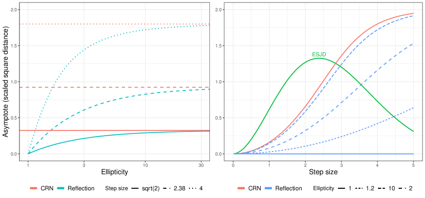
Figure 3: (Elliptical case.) Behaviour of $\lVert X_{t}-Y_{t}\rVert^{2}/(z_{-1}^{2}d)$ as $d,t\to\infty$ under the CRN and reflection couplings, according to asymptote (9). Left: Varying the ellipticity $\varepsilon$ and fixing the step size $l_{1}$. Right: Varying $l_{1}$ and fixing $\varepsilon$. The asymptote under the CRN coupling is unaffected by the ellipticity of the target; the ESJD is overlaid to provide context.

The above reasoning indicates that, when $\varepsilon>1$, $t\to\infty$ and $d$ is large,

$$\frac{1}{z_{-1}^{2}d}\lVert X_{t}-Y_{t}\rVert^{2}\approx 2(1-v),$$ (9)

where $v$ inherits the properties of Theorem 3. Irrespective of the ellipticity, the GCRN coupling brings the chains vanishingly close even in high dimension. For the CRN and reflection couplings, we illustrate the $d,t\to\infty$ asymptote (9) predicted by our theory in Figure 3. The values are to be compared with $2.0$, which corresponds to two stationary chains evolving independently. The CRN coupling performs as in the spherical case, we defer to Section 3.6 for further discussion. In contrast to the spherical case, and in contrast to the GCRN coupling, the contractivity of the reflection coupling breaks down in high enough dimension whenever there is any ellipticity ($\varepsilon>1$). Following Remark 1, the performance of the reflection coupling decays rapidly with the dimension when $l_{1}=\Theta_{d}(1)$ (so $l=\Theta_{d}(1)$), as this coupling does not contract the chains sufficiently. The contraction of the chains under the reflection coupling is satisfactory when a smaller scaling $l_{1}=o_{d}(1)$ (so $l=o_{d}(1)$) is employed. However, the mixing of the marginal RWM algorithm is then considerably slowed down in high dimensions. Neither the CRN nor the reflection couplings can be recommended for practical use when the target is high-dimensional and elliptical.

4.3 Optimality and scaling for GCRN coupling

Recall from Definition 1 that $\mathcal{I}$ is the set of couplings which are more amenable for practical implementation. We consider an objective which is qualitatively analogous to (6), and can be regarded as maximizing the contraction of the chains when the dimension is high:

$$\mathbb{E}\left[\eqref{eqn:innerprod-cross}\mid\frac{\lVert X_{t}\rVert_{\Omega_{(d)}^{2}}^{2}}{z_{1}^{2}d}=x_{1},\frac{\lVert Y_{t}\rVert_{\Omega_{(d)}^{2}}^{2}}{z_{1}^{2}d}=y_{1},\frac{\langle X_{t},Y_{t}\rangle_{\Omega_{(d)}^{2}}}{z_{1}^{2}d}=v_{1}\right].$$ (10)

Similarly to Theorem 2 in the spherical case, the GCRN coupling is asymptotically optimal among the class of couplings $\mathcal{I}$ in the elliptical targets as well.

Theorem 4 (Optimality of GCRN coupling).

Let $\widetilde{K}$ a coupling of the RWM kernels $(K(X_{t},\cdot),K(Y_{t},\cdot))$ of equation (1) with step size $h=ld^{-1/2}$. Then, for all $(x_{1},y_{1},v_{1})\in\mathcal{S}$,

$$\lim_{d\to\infty}\sup_{\widetilde{K}\in\mathcal{I}}\mathbb{E}\left[\eqref{eqn:innerprod-cross}\mid\frac{\lVert X_{t}\rVert_{\Omega_{(d)}^{2}}^{2}}{z_{1}^{2}d}=x_{1},\frac{\lVert Y_{t}\rVert_{\Omega_{(d)}^{2}}^{2}}{z_{1}^{2}d}=y_{1},\frac{\langle X_{t},Y_{t}\rangle_{\Omega_{(d)}^{2}}}{z_{1}^{2}d}=v_{1}\right]$$

is attained by the GCRN coupling.

We can also determine the step size which optimizes the objective (10) in the limit as $d\to\infty$. As in Section 3.6, we consider both chains to be (marginally) stationary. This qualitatively corresponds to $x_{1}=y_{1}=1$, in which case under the GCRN coupling it holds that

$$\lim_{d\to\infty}\left[\eqref{eqn:innerprod-cross}\mid\frac{\lVert X_{t}\rVert_{\Omega^{2}}^{2}}{z_{1}^{2}d}=1,\frac{\lVert Y_{t}\rVert_{\Omega^{2}}^{2}}{z_{1}^{2}d}=1,\frac{\langle X_{t},Y_{t}\rangle_{\Omega^{2}}}{z_{1}^{2}d}=v_{1}\right]=\frac{1}{z_{1}^{2}}l_{1}^{2}\Phi(-l_{1}/2).$$

The latter is proportional to the ESJD in the natural parameter $l_{1}$, and so the GCRN coupling scales exactly as the mixing of the marginal RWM algorithm does. The optimal step size under the GCRN coupling should be chosen such that approximately $l_{1}=2.38$ (so $l=2.38/z_{1}$), which corresponds to the well-known optimal acceptance rate of $23.4\%$ (sherlock2013optimal).

4.4 Numerical illustration

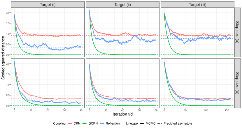
Figure 4: (Elliptical case.) MCMC traces and predicted long-time asymptotes (9) for the scaled squared distance between the chains $\lVert X_{t}-Y_{t}\rVert^{2}/(z_{-1}^{2}d)$, computed as described in Section 4.4.

We consider three targets $\pi=\mathcal{N}_{d}(0,\Sigma)$ of increasing ellipticity $\varepsilon$:

• $\Sigma_{ij}=0.5^{|i-j|}$: $\varepsilon=5/3$. This is an AR(1) process with correlation $0.5$ and unit noise.

• $\Sigma=\textup{diag}(\sigma^{2}_{1},\dots,\sigma^{2}_{d})$ where $\sigma^{2}_{1},\dots,\sigma^{2}_{d}\sim\chi^{2}_{3}$: $\varepsilon=3$.

• $\Sigma=\textup{diag}(1,24,1,24,\dots)$: $\varepsilon=25/4$.

We consider two step sizes (as in Section 3.3) for the natural parameter $l_{1}$: $(a)$ $l_{1}=2.38$ and $(b)$ $l_{1}=\sqrt{2}$. The former is optimal for the stationary phase (roberts1997weak), and Proposition 4 together with (christensen2005scaling) suggest that both are close to optimal for the transient phase. We perform MCMC in dimension $d=2000$, always starting both chains independently from the target.

The MCMC traces in Figure 4 resemble deterministic trajectories. Furthermore, as $t\to\infty$ the MCMC traces asymptote around (9), as indicated by the fixed point analysis of Section 4.2. For the reflection and CRN couplings, as the step size lowers, so does the asymptote. As the ellipticity of the target increases, so does the performance of the reflection coupling worsen, approaching the performance of the CRN coupling. The GCRN coupling performs excellently in all test cases, and universally outperforms the other two couplings, which fail to contract the chains to a negligible distance.

5 Applications of the GCRN coupling

Practical applications of couplings include estimating the convergence of MCMC algorithms (biswas2019estimating), estimating the bias of approximate inference procedures (biswas2019estimating) and unbiased estimation (jacob2020unbiased). In this section, we apply the GCRN coupling for estimating the convergence of RWM chains and estimating the bias of a Laplace approximation. We also use a natural extension to the GCRN coupling to quantify the convergence of the Hug and Hop algorithm (ludkin2022hug). We measure discrepancies by squared Wassestein distance and total variation distance,

$$\mathcal{W}_{2}^{2}(\mu,\nu)=\inf_{(X,Y)\in\Gamma(\mu,\nu)}\mathbb{E}[\lVert X-Y\rVert^{2}],\quad\textup{TVD}(\mu,\nu)=\inf_{(X,Y)\in\Gamma(\mu,\nu)}\mathbb{E}[\mathbbm{1}\{X\neq Y\}],$$

where $\Gamma(\mu,\nu)$ is the set of all couplings of $\mu,\nu$.

Our running example is the posterior distribution of a 360-dimensional stochastic volatility model (SVM; e.g. liu2001monte, Section 9.6.2) investigated in (papp2022paper). See Section D.3 for a description of the model.

5.1 Quantifying convergence

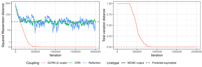
Figure 5: Convergence of the RWM targeting the SVM, when started from the prior. Upper bounds on the squared Wasserstein distance and total variation distance are computed with the two-scale coupling (using GCRN when the chains are sufficiently far apart). One MCMC trace of $\lVert X_{t+L}-Y_{t}\rVert^{2}$ is shown, for each of the CRN and reflection-maximal couplings, in the left plot.

We illustrate the effectiveness of the GCRN coupling at quantifying the convergence of the RWM beyond the Gaussian case, comparing it with the CRN and reflection-maximal (jacob2020unbiased, Section 4.1) couplings.

Before running coupled MCMC, we compute a Laplace approximation $\hat{\pi}=\mathcal{N}(\hat{\mu},\hat{\Sigma})$ using the optim function in R (r). This suggests the step size $h\approx 0.013$, which we employ and empirically verify as having an acceptance rate of $\approx 23\%$. The Laplace approximation also predicts the long-time limit of the squared distance between the chains for the CRN and reflection couplings, using the theory developed in Section 4.2. The ellipticity of the Laplace approximation is $\varepsilon\approx 9.6$, indicating that the target is highly eccentric and that the reflection-maximal coupling should perform poorly, corroborating empirical evidence in (papp2022paper).

We estimate upper bounds in total variation according to (biswas2019estimating), and bounds in squared Wasserstein distance according to the extension in papp2022paper. The framework in (biswas2019estimating) requires the chains to coalesce in finite time. As the GCRN coupling alone cannot produce exact meetings, we instead use a two-scale coupling employing the GCRN coupling kernel when the chains are at least $\lVert X_{t}-Y_{t}\rVert^{2}\geq\delta$ apart, and otherwise (when $\lVert X_{t}-Y_{t}\rVert^{2}<\delta$) employing a reflection-maximal coupling kernel. Two-scale couplings have previously been considered in e.g. (bou-rabee2020coupling; biswas2021coupling-based). A heuristic argument suggests that a scaling $\delta=O_{d}(1)$ is optimal in general, see Appendix E. The threshold $\delta=0.1$, chosen by a grid search, was found to give low meeting times on average. A lag of $L=2\times 10^{6}$ was chosen and $R=100$ independent replicates of coupled chains were run.

The numerical results are displayed in Figure 5. The reflection-maximal coupling is severely hindered by the ellipticity of the target, being unable to coalesce the chains in a feasible computational budget at the step size chosen for optimal mixing. The CRN coupling performs similarly, and the long-time behaviour of both couplings is accurately predicted by the results of Section 4.2. While the reflection-maximal coupling is capable of exact meetings, the probability of such meetings being proposed is effectively null at the squared distances in the figure. In contrast, the two-scale GCRN coupling effectively quantifies the convergence of the RWM algorithm, producing comparable bounds in total variation distance and squared Wasserstein distance, both of which suggest that the time-$t$ marginals of the Markov chains are virtually indistinguishable from the target by iteration $t=7.5\times 10^{5}$.

5.2 Quantifying bias

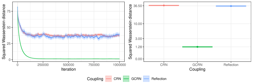
Figure 6: The bias of the Laplace approximation for the SVM. Under each coupling, $R=100$ pairs of coupled chains were run for $T=10^{6}$ iterations. Left: Trace plots of iteration-wise averages. Right: Point estimates of upper bounds on the squared Wasserstein distance, aggregated after discarding a burn-in of $S=3.5\times 10^{5}$ iterations. All averages are shown with $95\%$ confidence bands.

The GCRN coupling can also prove effective at quantifying the bias of approximate sampling procedures, following (biswas2021bounding). Motivated by the accuracy of the quantities inferred from the Laplace approximation of the SVM example of Section 5.1 (such as the optimal step size $h$ and the long-time behaviour under the CRN and reflection couplings), we employ the GCRN coupling to quantify the bias of this approximation in squared Wasserstein distance, comparing it with the CRN and reflection couplings.

We target the SVM posterior $\pi$ with the $X$-chain and its Laplace approximation $\hat{\pi}$ with the $Y$-chain. We start the two chains, independently, from the respective stationary distributions (SVM samples are obtained from long MCMC runs). If $n_{x}$ is the normalized gradient of the log-density of $\pi$ at $X$ and $\hat{n}_{y}$ is the normalized gradient of the log-density of the Laplace approximation $\hat{\pi}$ at $Y$, the GCRN coupling uses $X,Y$-proposals

$$Z_{x}=Z+(Z_{1}-n_{x}^{\top}Z_{1})n_{x},\quad Z_{y}=Z+(Z_{1}-\hat{n}_{y}^{\top}Z_{1})\hat{n}_{y},$$

where $Z\sim\mathcal{N}(0,I)$ and $Z_{1}\sim\mathcal{N}(0,1)$.

As shown in Figure 6, the reflection and CRN couplings give loose upper bounds which are ineffective at quantifying the bias of the Laplace approximation. Both bounds are more than $28$ times larger than the bound obtained by the GCRN coupling. In contrast, the GCRN coupling reveals that the Laplace approximation achieves a low bias of at most $1.3$ in squared Wasserstein distance (see Appendix F for an interpretation of this value).

5.3 Coupling the Hop kernel

Hug and Hop (H&H; ludkin2022hug) is a recently-proposed gradient-based algorithm that offers a competitive alternative to Hamiltonian Monte Carlo (HMC; duane1987hybrid; neal2011), while being geometrically ergodic on targets with light tails. In this section, we study the convergence of H&H with couplings.

H&H alternates between the skew-reversible Hug kernel, which proposes large moves by approximately traversing the same level set of the log-target, and the Hop kernel, which crosses between level sets by encouraging large moves in the gradient direction. Hop uses Gaussian proposals centered at the current state; the projection of the proposal onto the subspace orthogonal to the gradient is isotropic, and the projection onto the gradient uses a much larger scaling than each coordinate of its orthogonal counterpart. Due to its use of gradient information, the GCRN coupling is natural for the Hop kernel. One might expect the contractivity enjoyed by GCRN-coupled RWM kernels to carry over to GCRN-coupled Hop kernels.

We always use the same uniform random variable to accept coupled proposals, for both Hug and Hop. We couple Hug proposals with the same initial momenta (i.e. CRNs). The CRN coupling contracts Leapfrog-discretized HMC proposals (e.g. heng2019unbiased); due to the parallels of Hug and HMC, one might expect a CRN coupling to also contract Hug proposals. See Appendix G for a discussion on the contractivity of CRNs for Hug in high dimension. For Hop, we use a two-scale coupling which aims to contract the chains when far apart and allow for exact meetings when close together. When $\lVert Y_{t}-X_{t}\rVert^{2}\geq\delta$, we couple proposals according to the GCRN coupling

$$X_{p} =X_{t}+\frac{\lambda}{\lVert\nabla\log\pi(X_{t})\rVert}Z_{1}n_{x}+\frac{\mu}{\lVert\nabla\log\pi(X_{t})\rVert}\big{[}Z-\{Z^{\top}n_{x}\}n_{x}\big{]},$$

$$Y_{p} =Y_{t}+\frac{\lambda}{\lVert\nabla\log\pi(Y_{t})\rVert}Z_{1}n_{y}+\frac{\mu}{\lVert\nabla\log\pi(Y_{t})\rVert}\big{[}Z-\{Z^{\top}n_{y}\}n_{y}\big{]},$$

where $Z\sim\mathcal{N}_{d}(0_{d},I_{d})$ and $Z_{1}\sim\mathcal{N}_{1}(0,1)$ are independent. When $\lVert Y_{t}-X_{t}\rVert^{2}<\delta$, we sample the proposals from a maximal coupling with independent residuals, by rejection [e.g. thorisson2000, jacob2020unbiased, oleary2021maximal]. We choose $\delta=10^{-4}$ as a balance between the two couplings. See Appendix G for further discussion on the choice of threshold $\delta$, as well as a demonstration of and explanation of the failure of the CRN coupling for Hop. We choose Hop step sizes $(\lambda,\kappa)=(20,1)$, for an acceptance rate of $40\%$, and Hug integration time and bounce count $(T,B)=(0.5,10)$, for an acceptance rate of $75\%$. These are in line with tuning guidelines for H&H (ludkin2022hug, Section 2.8).

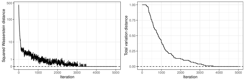
Figure 7: Estimated upper bounds on the convergence of the Hug and Hop algorithm targeting the SVM. $R=100$ coupled chains were used to compute the bounds, at a lag of $L=6\times 10^{3}$.

Estimated upper bounds on the convergence of H&H are displayed in Figure 7, which suggest that H&H converges more than two orders of magnitude faster than the RWM. More sophisticated couplings than the one considered here may sharpen these bounds. As the meeting times are relatively low, H&H with the proposed coupling may be suitable for unbiased MCMC in the framework of (jacob2020unbiased), and be competitive with Hamiltonian Monte Carlo in this framework (heng2019unbiased). As opposed to the HMC kernel, which must be combined with a potentially poorly mixing kernel to allow for exact meetings, H&H has the advantage of employing the Hop kernel which is amenable to couplings that allow the chains to meet exactly.

6 Discussion

Convergence estimation and analysis with couplings

Our theoretical and numerical results indicate that the GCRN coupling is effective at quantifying the convergence of the RWM algorithm targeting high-dimensional elliptical distributions. Within the framework of (biswas2019estimating) and when using the RWM algorithm, we recommend the use of the two-scale coupling as detailed in Section 5.1, swapping to a reflection-maximal coupling under a threshold $\delta=O_{d}(1)$ in squared distance. We have argued heuristically in Appendix E that the choice $\delta=O_{d}(1)$ optimally reduces the average meeting time. Moreover, this choice of threshold should be robust to increasing the dimension $d$, as the high-dimensional ODE behaviour of the GCRN coupling suggests that the chains contract to within $O_{d}(1)$ squared distance in the long-time limit.

The contractivity of the GCRN coupling may also provide a tool for obtaining analytical, quantitative convergence rates for the RWM algorithm, for instance in squared Wasserstein distance. Our initial attempts indicate that, in finite dimension, the GCRN coupling does not contract the chains sufficiently when they are near the mode, in the tails, or are extremely close to each other. As such, the GCRN coupling should be complemented with alternative tools, for instance a Lyapunov drift.

When the target is high-dimensional, the CRN coupling of the cannot be recommended for quantifying the convergence of the RWM. When the target is additionally elliptical, neither can the reflection (-maximal) coupling be. The problem the same in both scenarios: under step size scalings $l=\Theta_{d}(1)$, which lead to positive ESJDs and ensure that the marginal chains mix well, the chains cannot contract sufficiently well, which ultimately leads to extremely large meeting times. To ensure sufficient contraction, a much smaller step size scaling $l=o_{d}(1)$ should be used. RWM algorithms scaled so poorly are of little use in practice, and so any analysis of their convergence properties is of doubtful interest.

Unbiased MCMC

Our analysis has mixed consequences for unbiased MCMC (jacob2020unbiased). On the one hand, it indicates that gradient information should in general be included in the RWM coupling, otherwise the meeting times can increase quickly with the dimension the target. However, if gradient information is available, then it should be included in the proposal to produce a more efficient algorithm altogether, such as the Metropolis-adjusted Langevin algorithm (MALA).

On the other hand, our analysis also indicates scenarios where the RWM can be effective for unbiased MCMC. If the target can be preconditioned to be approximately spherical, then gradient information is unnecessary and the reflection-maximal coupling should work well in moderate dimension. In situations where cheap gradient surrogates are available, or the acceptance rate of the algorithm is low, the GCRN coupling may be used with relatively little overhead. Finally, in (heng2019unbiased) a contractive HMC coupling is mixed with an independent-residual maximal RWM coupling to allow for the chains to meet exactly. In high dimension, replacing this RWM coupling with a two-scale GCRN coupling will reduce meeting times at a negligible additional cost, thereby reducing the variance of the unbiased estimates.

Extension to other samplers

It may be possible to extend our analysis to other samplers, thereby motivating the design of better couplings. For instance, (christensen2005scaling) also derive ODE limits for MALA. However, just as a better coupling for the RWM requires gradient information, we postulate that improving upon the status-quo CRN coupling for MALA (e.g. eberle2014error) in high dimensions requires Hessian information.

Beyond the Gaussian case

While our analysis only concerns the Gaussian case, by Taylor expanding the log-acceptance ratio one can see that the GCRN coupling is a sensible choice for more general targets. We expect that the results concerning asymptotic optimality, optimal scaling, and the long-time limit of the scaled squared distance between the chains should extend to targets satisfying appropriate “shell” conditions, as in (sherlock2009optimal; sherlock2013optimal). However, our ODE limits depend on the Markov property of the processes under consideration, and so extending such results beyond the Gaussian case will require techniques different to the ones we have employed.

Additional related literature

In the context of MCMC, Markovian couplings have historically been used in theoretical analyses concerning (geometric) ergodicity (see roberts2004general, Section 3 for a review). While these analyses have primarily been of a qualitative nature, more recent theoretical analyses have used Markovian couplings to derive quantitative convergence rates (e.g. hairer2011asymptotic; eberle2014error; mangoubi2017rapid; durmus2019high; bou-rabee2020coupling). These latter works often implicitly consider implementable couplings which scale well with the dimension. Common random number (CRN) strategies, where both chains use the same proposal noise, have proven successful for gradient-based algorithms such as the unadjusted Langevin algorithm (durmus2019high), the Metropolis-adjusted Langevin algorithm (MALA; eberle2014error) and Hamiltonian Monte Carlo (mangoubi2017rapid; bou-rabee2020coupling). CRN couplings have also proven successful for algorithms designed for function spaces, such as preconditioned Crank-Nicholson (hairer2011asymptotic) and preconditioned MALA (eberle2014error).

In contrast to these works, we directly tackle the problem of designing couplings of the RWM algorithm which scale well with the dimension, and propose an asymptotic framework in which to do this. Quantitative convergence rates for the RWM algorithm (which are relatively well-known, e.g. chen2020fast) do not immediately follow from our analysis, however this does not preclude our proposed couplings also being for this purpose.

Appendix A Proofs

We make the following conventions in the proofs below. For simplicity of notation, we drop all subscripts and superscripts relating to the dimension $d$. For $x\in\mathbb{R}^{d}\setminus\{0\}$, we define $\widehat{x}=x/\lVert x\rVert$. When $x=0$ we choose $\widehat{x}$ arbitrarily (the final results carry through).

A.1 Auxiliary results

Lemma 4 below asserts that the function $1\land\exp(-x)$, which appears in the Metropolis-Hastings acceptance ratio, is 1-Lipschitz. This lemma also appears as roberts1997weak.

Lemma 4.

For all $x,y\in\mathbb{R}$ it holds that $|1\land\exp(-x)-1\land\exp(-y)|\leq|x-y|.$

Lemma 5 below (used in the proof of Lemma 1) translates the convergence in $L_{2}$ of $\chi^{2}_{d}/d\to 1$ as $d\to\infty$ into a convergence of expectations of interest.

Lemma 5.

Let $Z_{1},Z_{2}\sim\mathcal{N}(0,1)$ and $Z_{x}\sim\mathcal{N}_{d}(0,I_{d})$ be not necessarily independent. Then, uniformly over all $\alpha\in[0,\infty)$, it holds that

$$\lim_{d\to\infty}\mathbb{E}\big{[}Z_{2}1\land\exp\{-l\alpha Z_{1}-l^{2}\lVert Z_{x}\rVert^{2}/(2d)\}\big{]}=\mathbb{E}\big{[}Z_{2}1\land\exp\{-l\alpha Z_{1}-l^{2}/2\}\big{]}.$$

Proof.

Let $A_{d}=\lVert Z_{x}\rVert^{2}/d$. Since $\mathbb{E}A_{d}=1$ and $\textup{Var}A_{d}=2/d\to 0$ as $d\to\infty$, it holds that $A_{d}\to 1$ in $L_{2}$ as $d\to\infty$. Now, by the Cauchy-Schwarz inequality, we have that

$$\left[\mathbb{E}Z_{2}(1\land e^{-l\alpha Z_{1}-l^{2}A_{d}/2}-1\land e^{-l\alpha Z_{1}-l^{2}/2})\right]^{2} \leq\mathbb{E}[Z_{2}^{2}]\mathbb{E}[(1\land e^{-l\alpha Z_{1}-l^{2}A_{d}/2}-1\land e^{-l\alpha Z_{1}-l^{2}/2})^{2}]$$

$$\leq\mathbb{E}[Z_{2}^{2}]\mathbb{E}[(l^{2}A_{d}/2-l^{2}/2)^{2}]$$ (Lemma 4)

$$\to 0\quad\textup{as $d\to\infty$,}$$

using finally that $\mathbb{E}Z_{2}^{2}=1$ and that $l^{2}A_{d}/2\to l^{2}/2$ in $L_{2}$ as $d\to\infty$. The convergence is uniform over all $\alpha\in[0,\infty)$ as the dependence on $\alpha$ vanishes in the second line. This completes the proof. ∎

A.2 Proof of Proposition 1

For the CRN coupling, $Z_{x}=Z_{y}$ and so $\operatorname{Cov}(n_{x}^{\top}Z_{x},n_{y}^{\top}Z_{y})=\operatorname{Cov}(n_{x}^{\top}Z_{x},n_{y}^{\top}Z_{x})=n_{x}^{\top}n_{y}.$ For the reflection coupling, $Z_{y}=Z_{x}-2(e^{\top}Z_{x})e$ and so

$$\operatorname{Cov}(n_{x}^{\top}Z_{x},n_{y}^{\top}Z_{y}) =\operatorname{Cov}(n_{x}^{\top}Z_{x},n_{y}^{\top}Z_{x}-2(n_{y}^{\top}e)e^{\top}Z_{x})=n_{x}^{\top}n_{y}-2(n_{y}^{\top}e)(n_{x}^{\top}e).$$

For the GCRN coupling, $n_{x}^{\top}Z_{x}=n_{y}^{\top}Z_{y}$ and so $\operatorname{Cov}(n_{x}^{\top}Z_{x},n_{y}^{\top}Z_{y})=1.$ This concludes the proof.

A.3 Proof of Lemma 1

It is convenient to work with $\widetilde{W}=(\lVert X_{t}\rVert^{2}/d,\lVert Y_{t}\rVert^{2}/d,\widehat{X}_{t}^{\top}\widehat{Y}_{t})=(\alpha^{2},\beta^{2},\rho)$. In the original coordinate system, this corresponds to $x=\alpha^{2}$, $y=\beta^{2}$ and $v=\rho\alpha\beta$.

Conditionally on $\widehat{X}_{t}^{\top}\widehat{Y}_{t}=\rho$, it holds that $(Z_{1},Z_{2})=(\widehat{X}_{t}^{\top}Z,\widehat{Y}_{t}^{\top}Z)$ is a two-dimensional multivariate normal with unit component-wise variances and correlation $\rho$. Hence,

$$\mathbb{E}[\eqref{eqn:innerprod-x}\mid\widetilde{W}=(\alpha^{2},\beta^{2},\rho)]=l\beta\mathbb{E}\left(Z_{2}1\land e^{-l\alpha Z_{1}-l^{2}\lVert Z_{x}\rVert^{2}/(2d)}\right).$$

By Lemma 5 it follows that

$$\lim_{d\to\infty}\mathbb{E}[\eqref{eqn:innerprod-x}\mid\widetilde{W}=(\alpha^{2},\beta^{2},\rho)]=l\beta\mathbb{E}\left(Z_{2}1\land e^{-l\alpha Z_{1}-l^{2}/2}\right).$$ (11)

Moreover, fixing $B>0$, the convergence is uniform over all $\alpha\in[0,\infty)$ and $\beta\in[0,B]$.

Decompose $Z_{2}=\rho Z_{1}+\sqrt{1-\rho^{2}}Z_{*}$ where $Z_{*}\sim\mathcal{N}(0,1)$ is independent of $Z_{1}$. As the expectation (11) is over an odd function of $Z_{*}$, all terms involving $Z_{*}$ cancel out and it holds that

$$\lim_{d\to\infty}\mathbb{E}[\eqref{eqn:innerprod-x}\mid\widetilde{W}=(\alpha^{2},\beta^{2},\rho)]=\rho l\beta\mathbb{E}(Z_{1}1\land e^{-l\alpha Z_{1}-l^{2}/2})=-\rho\alpha\beta l^{2}\Phi(l/(2\alpha)-l\alpha),$$

where to compute the final expectation we have used Lemma 6. Rewrite the above expression in terms of $(x,y,v)=(\alpha^{2},\beta^{2},\rho\alpha\beta)$ and note that the constraint $\rho\in[-1,1]$ is equivalent to $v\in[-\sqrt{xy},\sqrt{xy}]$. This completes the proof of the first limit. The second limit follows by symmetry with the first, swapping $x$ and $y$. This completes the proof.

A.4 Proof of Lemma 2

Let $W=(\lVert X_{t}\rVert^{2},\lVert Y_{t}\rVert^{2},X_{t}^{\top}Y_{t})/d=(x,y,v)$. Conditionally on $\widehat{X}_{t}^{\top}\widehat{Y}_{t}$, it holds that $(Z_{1},Z_{2})=(\widehat{X}_{t}^{\top}Z_{x},\widehat{Y}_{t}^{\top}Z_{y})$ is a two-dimensional multivariate normal with unit component-wise variances and correlation $\rho(x,y,v)=\textup{Cov}(\widehat{X}_{t}^{\top}Z_{x},\widehat{Y}_{t}^{\top}Z_{y})$. Using that $n_{x}=-X_{t}/\lVert X_{t}\rVert$ and $n_{y}=-Y_{t}/\lVert Y_{t}\rVert$ are the normalized gradients, we evaluate $\rho$ using Proposition 1. For the GCRN coupling, $\rho_{\textup{gcrn}}=1$ by construction. For the CRN coupling it holds that $\rho_{\textup{crn}}=n_{x}^{\top}n_{y}=v/(xy)^{1/2}$. For the reflection coupling, the calculation is

$$\rho_{\textup{refl}} =n_{x}^{\top}n_{y}-2(n_{x}^{\top}e)(n_{y}^{\top}e)$$

$$=\frac{X_{t}^{\top}Y_{t}}{\lVert X_{t}\rVert\lVert Y_{t}\rVert}+2\frac{X_{t}^{\top}(X_{t}-Y_{t})}{\lVert X_{t}\rVert\lVert X_{t}-Y_{t}\rVert}\frac{Y_{t}^{\top}(Y_{t}-X_{t})}{\lVert Y_{t}\rVert\lVert X_{t}-Y_{t}\rVert}$$

$$=\frac{v}{(xy)^{1/2}}+2\frac{(x-v)(y-v)}{(xy)^{1/2}(x+y-2v)}=\frac{2xy-(x+y)v}{(xy)^{1/2}(x+y-2v)}.$$

Now, under all three couplings it holds that $h^{2}Z_{x}^{\top}Z_{y}\to l^{2}$ in $L_{2}$ as $d\to\infty$. In addition, $h^{2}\lVert Z_{x}\rVert^{2},h^{2}\lVert Z_{y}\rVert^{2}\to l^{2}$ in $L_{2}$ as $d\to\infty$. Arguing similarly to the proof of Lemma 5, and recalling that the same uniform random variable is used in both $B_{x}$ and $B_{y}$ for all couplings, by integrating over the increments $Z_{x},Z_{y}$ and the uniform random variable we obtain that

$$\lim_{d\to\infty}\mathbb{E}[\eqref{eqn:innerprod-cross}\mid W=(x,y,v)]=l^{2}\mathbb{E}_{(Z_{1},Z_{2})\sim\operatorname{BvN}(\rho)}[1\land e^{-lx^{1/2}Z_{1}-l^{2}/2}\land e^{-ly^{1/2}Z_{2}-l^{2}/2}].$$

Moreover, as in Lemma 5 the convergence is uniform over $(x,y,v)\in\mathcal{S}(X,Y)$, for all fixed $X,Y>0$.

A.5 Proof of Proposition 2

In what follows, let $\widetilde{\mathbb{E}}$ be the expectation conditional on $W_{t/d}=w=(x,y,z)^{\top}$. Let all suprema be over $w\in\mathcal{S}(X,Y)$.

Firstly, $\lVert W_{(t+1)/d}-W_{t/d}\rVert^{2}d^{2}=(\lVert X_{t+1}\rVert^{2}-\lVert X_{t}\rVert^{2})^{2}+(\lVert Y_{t+1}\rVert^{2}-\lVert Y_{t}\rVert^{2})^{2}+(X_{t+1}^{\top}Y_{t+1}-X_{t}^{\top}Y_{t})^{2}.$ It thus holds that

$$\sup\widetilde{\mathbb{E}}\lVert W_{(t+1)/d}-W_{t/d}\rVert^{2}d^{2}\leq \sup\widetilde{\mathbb{E}}(\lVert X_{t+1}\rVert^{2}-\lVert X_{t}\rVert^{2})^{2}+\sup\widetilde{\mathbb{E}}(\lVert Y_{t+1}\rVert^{2}-\lVert Y_{t}\rVert^{2})^{2}$$

$$+\sup\widetilde{\mathbb{E}}(X_{t+1}^{\top}Y_{t+1}-X_{t}^{\top}Y_{t})^{2}.$$

The first two terms are finite by christensen2005scaling. For the third term, using that $B_{x,y}\in[0,1]$ and $Z_{x}^{\top}Z_{y}\leq(\lVert Z_{x}\rVert^{2}+\lVert Z_{y}\rVert^{2})/2$, the following upper bound holds irrespectively of the coupling,

$$\widetilde{\mathbb{E}}(X_{t+1}^{\top}Y_{t+1}-X_{t}^{\top}Y_{t})^{2}\leq l^{2}(x^{2}+y^{2})\mathbb{E}Z^{2}+l^{4}\mathbb{E}\lVert Z_{x}\rVert^{4}/d^{2},$$

where $Z\sim\mathcal{N}_{1}(0,1)$. The limit supremum of the right hand-side is finite, which concludes the proof.

A.6 Proof of Theorem 1

The proof essentially mirrors that of christensen2005scaling. We show that the infinitesimal generator of the process $W^{d}$ converges to that of the ODE as $d\to\infty$. Textbook results concerning the convergence of stochastic processes then allow us to conclude.

We first recall some standard technical results. Let $\mathcal{S}\subset\mathbb{R}^{3}$ and let $\mathcal{C}_{c}^{\infty}(\mathcal{S})$ be the set of all infinitely differentiable functions $h:\mathcal{S}\to\mathbb{R}^{3}$ with compact support. Let $c:\mathcal{S}\to\mathcal{S}$ and let $w:[0,\infty)\to\mathcal{S}$ be the solution to the ordinary differential equation (ODE) $w^{\prime}(t)=c(w(t))$. Let the infinitesimal generator of $w^{\prime}(t)=c(w(t))$ be $G$, which we recall satisfies $Gh(x)=\nabla h(x)^{\top}c(x)$ for all $h\in\mathcal{C}_{c}^{\infty}(\mathcal{S})$ and $x\in\mathcal{S}$ (e.g. oksendal1998stochastic, Theorem 7.3.3). Moreover, the set $\mathcal{C}_{c}^{\infty}(\mathcal{S})$ is a core for the infinitesimal generator of the ODE $f^{\prime}(t)=c(f(t))$ (e.g. sato1999levy, Theorem 31.5, noting that an ODE is a Lévy process).

We now proceed to the main body of the proof, showing the convergence of the discrete time generator to the continuous time generator. Let $G^{(d)}$ be the discrete time infinitesimal generator of the process $W=W^{(d)}$. Let $h\in\mathcal{C}_{c}^{\infty}(\mathcal{S})$ and let $\mathbf{H}h$ denote the Hessian of $h$. For $w\in\mathcal{S}$, we have that

$$G^{(d)}h(w)= \mathbb{E}\left\{h(W_{(t+1)/d})-h(W_{t/d})\mid W_{t/d}=w\right\}d$$

$$= \mathbb{E}\left\{h(W_{(t+1)/d})-h(w)\mid W_{t/d}=w\right\}d$$

$$= \mathbb{E}\left\{\nabla h(w)^{\top}(W_{(t+1)/d}-w)\mid W_{t/d}=w\right\}d$$ (Taylor’s theorem)

$$+\frac{1}{2}\mathbb{E}\left\{(W_{(t+1)/d}-w)^{\top}\mathbf{H}h(W^{*})(W_{(t+1)/d}-w)\mid W_{t/d}=w\right\}d,$$

for some $W^{*}$ on the segment from $w$ to $W_{(t+1)/d}$. Since $h\in\mathcal{C}_{c}^{\infty}(\mathcal{S})$, it holds that $\sup_{x\in\mathcal{S}}\lVert\mathbf{H}h(x)\rVert_{\infty}\leq M<\infty$ for some $M\in\mathbb{R}$, where $\lVert\cdot\rVert_{\infty}$ is the sup-norm. Using that $(W_{(t+1)/d}-w)^{\top}\mathbf{H}h(W^{*})(W_{(t+1)/d}-w)\leq\lVert\mathbf{H}h(W^{*})\rVert_{\infty}\lVert W_{(t+1)/d}-w\rVert^{2}\leq M\lVert W_{(t+1)/d}-w\rVert^{2}$, then applying Corollary 1 and Proposition 2, we obtain that

$$\lim_{d\to\infty}\sup_{w\in\mathcal{S}(X,Y)}\left|G^{(d)}h(w)-Gh(w)\right|=0.$$ (12)

The limit (12) is analogous to christensen2005scaling.

The final part of the proof extends the convergence of the infintesimals (12) to the weak convergence of the stochastic processes. Since $h\in\mathcal{C}_{c}^{\infty}(\mathcal{S})$, we can instead take the supremum in (12) over the whole of $\mathcal{S}$. Moreover, $\mathcal{C}_{c}^{\infty}(\mathcal{S})$ is a core for $G$, so the limit (12) is equivalent to point $(i)$ of kallenberg2021foundations. Point $(iv)$ of the same theorem takes us from the convergence of the infinitesimal generator to the weak convergence of the process. This completes the proof.

A.7 Proof of Proposition 3

Fixed points

Firstly, let us determine the fixed points. For each of the first two coordinates, the only fixed point is $a(1)=0$. The fixed points of the three-dimensional ODE (IP) are therefore the solutions $(x,y,v)^{\top}=(1,1,v)^{\top}$ of

$$b(1,1,v)/l^{2}=g(1,1,v)-2\Phi(-l/2)v=0,\quad\textup{with }v\in[0,1].$$ (13)

For both the GCRN and reflection couplings, $g(1,1,v)=2\Phi(-l/2)$, and so the unique fixed point is $v_{\textup{gcrn}}=v_{\textup{refl}}=1$. For the CRN coupling, $g(1,1,v)=h(v)$ with $v$ defined as in Lemma 7. It holds that $h$ is continuous, $h(0)>0$ and $h(1)=2\Phi(-l/2)$, and additionally by Lemma 7 that $h$ is differentiable and convex on $[0,1)$ and $\lim_{v\nearrow 1}\partial_{v}h(v)=\infty$. Equation (13) therefore has two solutions, $v_{\textup{crn}}\in(0,1)$ and $v=1$, which are the fixed points of the ODE (IP) under the CRN coupling.

Stability

With the fixed points in hand, we show the (asymptotic, exponential) stability of these fixed points by using standard techniques from linear stability analysis. Under each coupling, $c\in\mathcal{C}^{1}$ in the interior of $\mathcal{S}$, so the Jacobian of $c$ is well-defined in the interior of $\mathcal{S}$ and the stability of the fixed points of the system (IP) is determined by the signs of the eigenvalues of the Jacobian. The first two coordinates of the three-dimensional (IP) are univariate autonomous ODEs (both determined by $a$) so the eigenvalues of the Jacobian are simply its diagonal entries $(\partial_{x}a(x),\partial_{y}a(y),\partial_{v}b(x,y,v))^{\top}$.

Focusing on the first coordinate, by differentiating $a$ we have that

$$a^{\prime}(x)/l^{2}= (-2+\frac{l^{2}}{2}-l^{2}x)e^{l^{2}(x-1)/2}\Phi(\frac{l}{2x^{1/2}}-lx^{1/2})$$

$$+(1-2x)e^{l^{2}(x-1)/2}(\frac{l}{4x^{3/2}}-\frac{l}{2x^{1/2}})\phi(\frac{l}{2x^{1/2}}-lx^{1/2})+\frac{l}{4x^{3/2}}\phi(-\frac{l}{2x^{1/2}}).$$

In particular, at the fixed point, $a^{\prime}(1)/l^{2}=(l/2)\phi(-l/2)-2(1+l^{2}/4)\Phi(-l/2)$. Since $\lim_{l\to\infty}a^{\prime}(1)/l^{2}=0$, to show that $a^{\prime}(1)<0$ it suffices to show that $\partial_{l}(a^{\prime}(1)/l^{2})>0$ for all $l>0$. Indeed, $\partial_{l}(a^{\prime}(1)/l^{2})=2\phi(-l/2)-l\Phi(-l/2)>0$ for all $l>0$ since $\phi(-r)/r>\Phi(-r)$ for all $r>0$. It follows that $a^{\prime}(1)<0$. Overall, the unique fixed point $x=1$ of the autonomous ODE in the first coordinate is asymptotically stable. Similarly, $y=1$ is asymptotically stable in the second coordinate.

Due to the stability of the first two autonomous coordinates, the stability of the fixed points of the system (IP) is fully determined by the stability in the (coupling-specific) third coordinate. For both the GCRN and reflection couplings $\partial_{v}b(1,1,v)=\partial_{v}g(1,1,v)-2\Phi(-l/2)=-2\Phi(-l/2)<0$, so the unique fixed point $v_{\textup{gcrn}}=v_{\textup{refl}}=1$ is stable. For the CRN coupling, $\partial_{v}b(1,1,v)=\partial_{v}h(v)-2\Phi(-l/2)$, where $h$ is as in Lemma 7. By Lemma 7, $\lim_{v\nearrow 1}\partial_{v}b(1,1,v)=\infty$ and so the fixed point at $v=1$ is unstable. Since $b(1,1,v)$ is a convex function of $v$, and $b(1,1,0)<0$, $b(1,1,v_{\textup{crn}})=0$ with $v_{\textup{crn}}\in(0,1)$ and $b(1,1,1)=0$, it must hold that $\partial_{v}b(1,1,v_{\textup{crn}})<0$. Hence the fixed point $v_{\textup{crn}}$ is stable.

Behaviour of $v_{\textup{crn}}$ with $l$

As established above, the stable fixed point for the CRN coupling is the (unique) solution of $h(v)/h(1)=v$ which falls in $(0,1)$. By Lemma 8, it follows that $\lim_{l\to 0}v_{\textup{crn}}=1$ and $\lim_{l\to\infty}v_{\textup{crn}}=0$. (One can argue these limits by contradiction.) This concludes the proof.

A.8 Proof of Theorem 2

Let $\widetilde{\mathbb{E}}$ represent the expectation conditional on $(\lVert X_{t}\rVert^{2}/d=x,\lVert Y_{t}\rVert^{2}/d=y,X_{t}^{\top}Y_{t}/d=v)$. Define the $\mathcal{N}(0,1)$ random variables $Z_{1}=\widehat{X}_{t}^{\top}Z_{x}$, $Z_{2}=\widehat{Y}_{t}^{\top}Z_{y}$. Under any coupling in $\widetilde{K}\in\mathcal{I}$, by reasoning similarly to the proof of Lemma 5 we obtain that

$$\widetilde{\mathbb{E}}[\eqref{eqn:innerprod-cross}]=\mathbb{E}[1\land e^{-lx^{1/2}Z_{1}-l^{2}/2}\land e^{-ly^{1/2}Z_{2}-l^{2}/2}]+o_{d}(1),$$ (14)

where the convergence of the remainder $o_{d}(1)$ to $0$ can be controlled independently of the coupling $\widetilde{K}$ used. We shall show that the RHS of (14) is maximized when $Z_{1}=Z_{2}$. Let $L_{1}=1\land e^{-lx^{1/2}Z_{1}-l^{2}/2}$ and $L_{2}=1\land e^{-ly^{1/2}Z_{2}-l^{2}/2}$ (these are truncated log-normal random variables). By villani2003topics, the minimum of $\mathbb{E}|L_{1}-L_{2}|$ over all couplings $(L_{1},L_{2})$ is attained when $L_{1}$ and $L_{2}$ are coupled by pairing order statistics. One such coupling can be obtained by setting $Z_{1}=Z_{2}$. Since $\mathbb{E}|L_{1}-L_{2}|=\mathbb{E}L_{1}+\mathbb{E}L_{1}-2\mathbb{E}L_{1}\land L_{2}$, and $\mathbb{E}L_{1},\mathbb{E}L_{2}$ are invariant to the coupling of $L_{1}$ and $L_{2}$, the choice $Z_{1}=Z_{2}$ also maximizes $\mathbb{E}L_{1}\land L_{2}$. From (14) it follows that

$$\lim_{d\to\infty}\sup_{\widetilde{K}\in\mathcal{I}}\widetilde{\mathbb{E}}[\eqref{eqn:innerprod-cross}]\leq\mathbb{E}[1\land e^{-lx^{1/2}Z_{1}-l^{2}/2}\land e^{-ly^{1/2}Z_{1}-l^{2}/2}].$$

By Lemma 2, the RHS is $\lim_{d\to\infty}\widetilde{\mathbb{E}}[\eqref{eqn:innerprod-cross}]$ under the GCRN coupling. This concludes the proof.

A.9 Proof of Lemma 3

For the GCRN coupling, $\rho_{\textup{gcrn}}=1$ by definition. Recall now that the gradient at $X_{t}$ is $-\Omega X_{t}$. For the CRN coupling, $\rho_{\textup{crn}}=n_{x}^{\top}n_{y}=\langle X_{t},Y_{t}\rangle_{\Omega^{2}}/(\lVert X_{t}\rVert_{\Omega^{2}}\lVert Y_{t}\rVert_{\Omega^{2}})=v_{1}/(x_{1}y_{1})^{1/2}$. For the reflection coupling,

$$\rho_{\textup{refl}}=n_{x}^{\top}n_{y}-2(n_{y}^{\top}e)(n_{x}^{\top}e)=\rho_{\textup{crn}}+2\frac{n_{x}^{\top}(X_{t}-Y_{t})n_{y}^{\top}(Y_{t}-X_{t})}{\lVert X_{t}-Y_{t}\rVert^{2}}.$$

We have that $n_{x}^{\top}(X_{t}-Y_{t})=-(\lVert X_{t}\rVert^{2}_{\Omega}-\lVert Y_{t}\rVert^{2}_{\Omega})/\lVert X_{t}\rVert_{\Omega^{2}}=-(x_{0}-v_{0})/x_{1}^{1/2}$ and similarly $n_{x}^{\top}(Y_{t}-X_{t})=-(y_{0}-v_{0})/y_{1}^{1/2}$. Finally, using that $\lVert X_{t}-Y_{t}\rVert^{2}=x_{-1}+y_{-1}-2v_{-1}$ concludes the proof.

A.10 Proof of Proposition 4

In the elliptical case, the acceptance Bernoulli random variable for the $X$-chain is $B_{x}=\mathbbm{1}\{U\leq e^{-h\langle X_{t},Z_{x}\rangle_{\Omega}-h^{2}\lVert Z_{x}\rVert_{\Omega}^{2}/2}\}$. Recalling that a synchronous uniform acceptance variable is used for all couplings, the analogous expression for the $Y$-chain is $B_{y}=\mathbbm{1}\{U\leq e^{-h\langle X_{t},Z_{y}\rangle_{\Omega}-h^{2}\lVert Z_{y}\rVert_{\Omega}^{2}/2}\}$. We shall use these expressions together with the expansions

$$\lVert X_{t+1}\rVert_{\Omega^{k}}^{2}-\lVert X_{t}\rVert_{\Omega^{k}}^{2}= \left\{2h\langle X_{t},Z_{x}\rangle_{\Omega^{k}}+h^{2}\lVert Z_{x}\rVert_{\Omega^{k}}^{2}\right\}B_{x}$$ (15)

$$\langle X_{t+1},Y_{t+1}\rangle_{\Omega^{k}}-\langle X_{t},Y_{t}\rangle_{\Omega^{k}}= h\langle Y_{t},Z_{x}\rangle_{\Omega^{k}}B_{x}+h\langle X_{t},Z_{y}\rangle_{\Omega^{k}}B_{y}+h^{2}\langle Z_{x},Z_{y}\rangle_{\Omega^{k}}B_{x}B_{y}.$$ (16)

Conditionally on $(\lVert X_{t}\rVert_{\Omega^{2k}}^{2},\lVert X_{t}\rVert_{\Omega^{2}}^{2},\lVert X_{t}\rVert_{\Omega^{k+1}}^{2})$, the random variable $(h\langle X_{t},Z_{x}\rangle_{\Omega^{k}},h\langle X_{t},Z_{x}\rangle_{\Omega})^{\top}$ is distributed as $\operatorname{BvN}\{h^{2}\lVert X_{t}\rVert_{\Omega^{2k}}^{2},h^{2}\lVert X_{t}\rVert_{\Omega^{2}}^{2};h^{2}\lVert X_{t}\rVert_{\Omega^{k+1}}^{2}\}=\operatorname{BvN}\{l_{2k-1}^{2}x_{2k-1},l_{1}^{2}x_{1};l_{k}^{2}x_{k}\}$, where for this proof only $\operatorname{BvN}(a,b;c)$ denotes a bivariate normal distribution with variances $a,b$ and covariance $c$. Similarly, conditionally on $(\lVert Y_{t}\rVert_{\Omega^{2k}}^{2},\lVert X_{t}\rVert_{\Omega^{2}}^{2},\langle Y_{t},X_{t}\rangle_{\Omega^{k+1}})$, the random variable $(h\langle Y_{t},Z_{x}\rangle_{\Omega^{k}},h\langle X_{t},Z_{x}\rangle_{\Omega})^{\top}$ is distributed as $\operatorname{BvN}\{l_{2k-1}^{2}y_{2k-1},l_{1}^{2}x_{1};l_{k}^{2}v_{k}\}$.

For the first conditional expectation, we have that

$$\lim_{d\to\infty} \widetilde{\mathbb{E}}\left[\lVert X_{t+1}\rVert_{\Omega^{k}}^{2}-\lVert X_{t}\rVert_{\Omega^{k}}^{2}\right]=\lim_{d\to\infty}\widetilde{\mathbb{E}}\left[\left(2h\langle X_{t},Z_{x}\rangle_{\Omega^{k}}+h^{2}\lVert Z_{x}\rVert_{\Omega^{k}}^{2}\right)\left(1\land e^{-h\langle X_{t},Z_{x}\rangle_{\Omega}-h^{2}\lVert Z_{x}\rVert_{\Omega}^{2}/2}\right)\right]$$

$$=\mathbb{E}_{Z\sim\mathcal{N}(0,1)}\left[(2l_{k}^{2}x_{k}Z+l_{k}^{2})\left(1\land e^{-l_{1}x_{1}^{1/2}Z-l_{1}^{2}/2}\right)\right]$$

$$=l_{k}^{2}\left\{-2x_{k}e^{l_{1}^{2}(x_{1}-1)/2}\Phi(\frac{l_{1}}{2x_{1}^{1/2}}-l_{1}x_{1}^{1/2})+\Phi(-\frac{l_{1}}{2x_{1}^{1/2}})+e^{l_{1}^{2}(x_{1}-1)/2}\Phi(\frac{l_{1}}{2x_{1}^{1/2}}-l_{1}x_{1}^{1/2})\right\}$$

$$=l_{k}^{2}\left\{(1-2x_{k})e^{l_{1}^{2}(x_{1}-1)/2}\Phi(\frac{l_{1}}{2x_{1}^{1/2}}-l_{1}x_{1}^{1/2})+\Phi(-\frac{l_{1}}{2x_{1}^{1/2}})\right\},$$

where the second line follows by using (15) then arguing similarly to the proof of Lemma 1 (using Assumption 1 and the bivariate normal random variables made explicit above); in the third line we have used Lemma 6 with the changes of variables $\alpha,\beta\leftarrow x_{1}^{1/2}$ and $l\leftarrow l_{1}$. The expression for $\lim_{d\to\infty}\widetilde{\mathbb{E}}\left[\lVert Y_{t+1}\rVert_{\Omega^{k}}^{2}-\lVert Y_{t}\rVert_{\Omega^{k}}^{2}\right]$ follows by symmetry.

We now turn to the third conditional expectation. Arguing as before, we have that

$$\lim_{d\to\infty}\widetilde{\mathbb{E}}\left[h\langle Y_{t},Z_{x}\rangle_{\Omega^{k}}B_{x}\right] =\mathbb{E}_{Z\sim\mathcal{N}(0,1)}\left[l_{k}^{2}v_{k}Z\Big{(}1\land e^{-l_{1}x_{1}^{1/2}Z-l_{1}^{2}/2}\Big{)}\right]$$

$$=-l_{k}^{2}v_{k}e^{l_{1}^{2}(x_{1}-1)/2}\Phi(\frac{l_{1}}{2x_{1}^{1/2}}-l_{1}x_{1}^{1/2}),$$

where the final expression follows by Lemma 6. By symmetry, $\lim_{d\to\infty}\widetilde{\mathbb{E}}\left[h\langle X_{t},Z_{y}\rangle_{\Omega^{k}}B_{y}\right]=-l_{k}^{2}v_{k}e^{l_{1}^{2}(y_{1}-1)/2}\Phi\big{(}l_{1}/(2y_{1}^{1/2})-l_{1}y_{1}^{1/2}\big{)}$. Finally, by Assumption 1, under all three couplings it holds that $\lim_{d\to\infty}h^{2}\langle Z_{x},Z_{y}\rangle_{\Omega^{k}}=l_{k}^{2}$ in $L_{2}$ for all $k$, since the contribution from the at most $2$ components of $Z_{x},Z_{y}$ which are different is negligible in the expression. Hence, we have that

$$\lim_{d\to\infty}\widetilde{\mathbb{E}}[h^{2}\langle Z_{x},Z_{y}\rangle_{\Omega^{k}}B_{x}B_{y}]=l_{k}^{2}\mathbb{E}_{(Z_{1},Z_{2})\sim\operatorname{BvN}(\rho)}\left[1\land e^{-l_{1}x_{1}^{1/2}Z_{1}-l_{1}^{2}/2}\land e^{-l_{1}y_{1}^{1/2}Z_{2}-l_{1}^{2}/2}\right],$$

where the correlation $\rho$ depends on the coupling as in Lemma 3. The desired expression follows by gathering terms, which concludes the proof.

A.11 Proof of Proposition 5

This essentially follows the proof of Proposition 2. Expanding $z_{k-1}^{4}\lVert\widetilde{W}_{(t+1)/d,k}-\widetilde{W}_{t/d,k}\rVert^{2}d^{2}$, we have that

$$z_{k-1}^{4}\sup\widetilde{\mathbb{E}}\lVert\widetilde{W}_{(t+1)/d,k}-\widetilde{W}_{t/d,k}\rVert^{2}d^{2}\leq \sup\widetilde{\mathbb{E}}(\lVert X_{t+1}\rVert^{2}_{\Omega^{k}}-\lVert X_{t}\rVert^{2}_{\Omega^{k}})^{2}$$

$$+\sup\widetilde{\mathbb{E}}(\lVert Y_{t+1}\rVert^{2}_{\Omega^{k}}-\lVert Y_{t}\rVert^{2}_{\Omega^{k}})^{2}$$

$$+\sup\widetilde{\mathbb{E}}(\langle X_{t+1},Y_{t+1}\rangle_{\Omega^{k}}-\langle X_{t},Y_{t}\rangle_{\Omega^{k}})^{2}.$$

It is therefore sufficient to show that the limit suprema of each of the three terms on the right-hand-side is finite.

For the first term, using firstly the expansion (15) in the proof of Proposition 4 and that $|B_{x}|\leq 1$, we have that

$$\widetilde{\mathbb{E}}(\lVert X_{t+1}\rVert_{\Omega^{k}}^{2}-\lVert X_{t}\rVert_{\Omega^{k}}^{2})^{2} \leq\widetilde{\mathbb{E}}\left(2h\langle X_{t},Z_{x}\rangle_{\Omega^{k}}+h^{2}\lVert Z_{x}\rVert_{\Omega^{k}}^{2}\right)^{2}$$

$$\leq 8h^{2}\widetilde{\mathbb{E}}\langle X_{t},Z_{x}\rangle_{\Omega^{k}}^{2}+2h^{4}\lVert Z_{x}\rVert_{\Omega^{k}}^{4} (x+y)^{2}\leq 2(x^{2}+y^{2})$$ (as )

$$=8h^{2}\lVert X_{t}\rVert^{2}_{\Omega^{2k}}+2h^{4}\mathbb{E}\lVert Z_{x}\rVert_{\Omega^{k}}^{4},$$

using finally that or any $Z_{x}\sim N(0,I_{d})$, it holds that $E[Z_{x}Z_{x}^{\top}]=I_{d}$, so $\widetilde{\mathbb{E}}\langle X_{t},Z_{x}\rangle_{\Omega^{k}}^{2}=\widetilde{\mathbb{E}}(\Omega^{k}X_{t})^{\top}Z_{x}Z_{x}^{\top}(\Omega^{k}X_{t})=\lVert X_{t}\rVert^{2}_{\Omega^{2k}}$. By Assumption 1, the limit (as $d\to\infty$) supremum (over any coordinate-wise compact set of values for $\widetilde{W}_{t/d,k}$, and therefore a compact set of values for $h^{2}\lVert X_{t}\rVert^{2}_{\Omega^{2k}}$) of the RHS is bounded. The second term follows by symmetry. For the third term, using firstly the expansion (16) in the proof of Proposition 4, that $|B_{x}|,|B_{y}|\leq 1$, and the elementary inequality $(x+y+z)^{2}\leq 3(x^{2}+y^{2}+z^{2})$ (a consequence of Cauchy-Schwarz), we have that

$$\widetilde{\mathbb{E}}(\langle X_{t+1},Y_{t+1}\rangle_{\Omega^{k}}-\langle X_{t},Y_{t}\rangle_{\Omega^{k}})^{2} \leq 3\widetilde{\mathbb{E}}(h\langle Y_{t},Z_{x}\rangle_{\Omega^{k}})^{2}+3\widetilde{\mathbb{E}}(h\langle X_{t},Z_{y}\rangle_{\Omega^{k}})^{2}+3\widetilde{\mathbb{E}}(h^{2}\langle Z_{x},Z_{y}\rangle_{\Omega^{k}})^{2}$$

$$\leq 3h^{2}\lVert Y_{t}\rVert_{\Omega^{2k}}^{2}+3h^{2}\lVert X_{t}\rVert_{\Omega^{2k}}^{2}+(3/2)\mathbb{E}(h^{2}\lVert Z_{x}\rVert_{\Omega^{k}}^{2}+h^{2}\lVert Z_{y}\rVert_{\Omega^{k}}^{2})^{2}$$

$$\leq 3h^{2}\lVert Y_{t}\rVert_{\Omega^{2k}}^{2}+3h^{2}\lVert X_{t}\rVert_{\Omega^{2k}}^{2}+3h^{4}\mathbb{E}\lVert Z_{x}\rVert_{\Omega^{k}}^{4},$$

where in the second line we have used that $\widetilde{\mathbb{E}}(h\langle Y_{t},Z_{x}\rangle_{\Omega^{k}})^{2}=\lVert Y_{t}\rVert_{\Omega^{2k}}^{2}$, $\widetilde{\mathbb{E}}(h\langle X_{t},Z_{y}\rangle_{\Omega^{k}})^{2}=\lVert X_{t}\rVert_{\Omega^{2k}}^{2}$, and $\langle Z_{x},Z_{y}\rangle_{\Omega^{k}}\leq(\lVert Z_{x}\rVert_{\Omega^{k}}^{2}+\lVert Z_{y}\rVert_{\Omega^{k}}^{2})/2$. The bound on the RHS is independent of the coupling, and arguing as before its limit supremum is bounded. This concludes the proof.

A.12 Proof of Theorem 3

We drop the subscript from $l_{1}$. Let $h$ be as in Lemma 7. We recall that $h(\rho)$ is increasing, convex, has unbounded gradient as $\rho\nearrow 1$, $h(0)>0$ and that $h(1)=2\Phi(-l/2)$ by Lemma 6.

The solutions and their stability

For all couplings, Equation (8) reduces to

$$h(\rho)-h(1)v=0.$$

For the GCRN coupling, $\rho=1$ so Equation (8) has the unique solution $v_{\textup{gcrn}}=1$. For the CRN coupling, $\rho=v$ and the coupling is invariant to $\varepsilon$; the proof therefore follows that of Proposition 3, and we obtain the unstable solution $v_{u}=1$ and the stable solution $v_{\textup{crn}}=1$. For the reflection coupling, we reparametrize Equation (8) by $\rho=v+(1-v)/\varepsilon$ to obtain

$$f(\rho)=h(\rho)-h(1)\frac{\rho-1/\varepsilon}{1-1/\varepsilon}=0.$$ (17)

From the properties of $h$, it holds that $f$ is convex, and $f(1)=0$, $f(1/\varepsilon)>0$. Hence, Equation (17) has the unique solutions $\rho_{\textup{refl}}\in(1/\varepsilon,1)$ and $\rho_{u}=1$. Moreover, from the properties of $h$ it holds that $\partial_{\rho}f(\rho_{\textup{refl}})<0$, so this solution is stable, and that $\lim_{\rho\nearrow 1}\partial_{\rho}f(\rho)=\infty$, so this solution is unstable. Changing variables back to $v=(\rho-1/\varepsilon)/(1-1/\varepsilon)$ yields the unique solutions $v_{\textup{refl}}\in(0,1)$ and $v_{u}=1$ to Equation (8), the former of which is stable and the latter of which is unstable.

Behaviour with ellipticity

We now turn to the behaviour of $v_{\textup{refl}}$ as the ellipticity $\varepsilon$ is varied. The LHS of Equation (8) is $g(v;\varepsilon)=h(v+(1-v)/\varepsilon)-h(1)v$. Since $g(v;1)=h(1)(1-v)$, it holds that $\lim_{\varepsilon\to 1}v_{\textup{refl}}=1$. Since $\lim_{\varepsilon\to\infty}g(v;\varepsilon)=h(v)-h(1)v$, it holds that $\lim_{\varepsilon\to\infty}v_{\textup{refl}}=v_{\textup{crn}}$. Finally, $g(v;\varepsilon)$ is decreasing in $\varepsilon$, so the properties of $h$ imply that $v_{\textup{refl}}$ must also be decreasing in $\varepsilon$.

Showing $v_{\textup{refl}}>v_{\textup{crn}}$

We argue this by contradiction. Suppose that $v_{\textup{refl}}\leq v_{\textup{crn}}$. From Equation (8) under both the reflection and CRN couplings, it follows that $h(v_{\textup{refl}}+(1-v_{\textup{refl}})/\varepsilon)\leq h(v_{\textup{crn}})$. Since $h$ is increasing, it holds that $v_{\textup{refl}}+(1-v_{\textup{refl}})/\varepsilon\leq v_{\textup{crn}}$. Now, due to the properties of $h$ it holds that $h(w)\geq h(1)w$ for any $w\in[0,v_{\textup{crn}}]$, so it must also hold that $h(v_{\textup{refl}}+(1-v_{\textup{refl}})/\varepsilon)\geq h(1)[v_{\textup{refl}}+(1-v_{\textup{refl}})/\varepsilon]$. Hence, using Equation (8) under the reflection coupling, it holds that $v_{\textup{refl}}\geq v_{\textup{refl}}+(1-v_{\textup{refl}})/\varepsilon$. As we have assumed that $v_{\textup{refl}}\leq v_{\textup{crn}}$, we have arrived at a contradiction. It follows that $v_{\textup{refl}}>v_{\textup{crn}}$.

Behaviour with step size

Similarly to the proof of Proposition 3, it follows from Lemma 8 that $v_{\textup{refl}},v_{\textup{crn}}$ are decreasing in $l$ and that $\lim_{l\to\infty}v_{\textup{refl}}=\lim_{l\to\infty}v_{\textup{crn}}=0$ and $\lim_{l\to 0}v_{\textup{refl}}=\lim_{l\to 0}v_{\textup{crn}}=1$. This completes the proof.

A.13 Proof of Theorem 4

This is essentially identical to the proof of Theorem 2 and is therefore omitted.

Appendix B Additional lemmas

B.1 Explicit integrals

The following explicit integrals will turn up repeatedly in our analysis, including the derivation of the ODE limit for the GCRN coupling.

Lemma 6.

Let $\alpha,\beta,l>0$ and $Z\sim\mathcal{N}(0,1)$. Then, it holds that

$$\mathbb{E}[Z1\land e^{-l\alpha Z-l^{2}/2}] =-l\alpha e^{l^{2}(\alpha^{2}-1)/2}\Phi(\frac{l}{2\alpha}-l\alpha).$$

$$\mathbb{E}[1\land e^{-l\alpha Z-l^{2}/2}\land e^{-l\beta Z-l^{2}/2}] =\Phi(-\frac{l}{2m})+e^{l^{2}(m^{2}-1)/2}\left\{\Phi(\frac{l}{2m}-lm)-\Phi(-lm)\right\}+e^{l^{2}(M^{2}-1)/2}\Phi(-lM),$$

where $m=\alpha\land\beta$ and $M=\alpha\lor\beta$.

Proof.

For the first expectation, let $E_{1}=\mathbb{E}Z1\land e^{-l\alpha Z-l^{2}/2}$. Firstly, since $z\phi(z)=-{\mathrm{d}\phi(z)}/{\mathrm{d}z}$, it holds that $\int_{a}^{b}z\phi(z)\mathrm{d}z=-\int_{a}^{b}\mathrm{d}\phi(z)=\phi(a)-\phi(b).$ Thus,

$$E_{1} =\int_{-\infty}^{-l/(2\alpha)}z\phi(z)\mathrm{d}z+\int_{-l/(2\alpha)}^{\infty}ze^{-l\alpha z-l^{2}/2}\phi(z)\mathrm{d}z$$

$$=-\phi(-\frac{l}{2\alpha})+e^{l^{2}(\alpha^{2}-1)/2}\int_{-l/(2\alpha)}^{\infty}z\phi(z+l\alpha)\mathrm{d}z$$

$$=-\phi(-\frac{l}{2\alpha})+e^{l^{2}(\alpha^{2}-1)/2}\left\{\int_{-l/(2\alpha)}^{\infty}(z+l\alpha)\phi(z+l\alpha)\mathrm{d}z-l\alpha\int_{-l/(2\alpha)}^{\infty}\phi(z+l\alpha)\mathrm{d}z\right\}$$

$$=-\phi(-\frac{l}{2\alpha})+e^{l^{2}(\alpha^{2}-1)/2}\left\{\int_{-l/(2\alpha)+l\alpha}^{\infty}z\phi(z)\mathrm{d}z-l\alpha\int_{-l/(2\alpha)+l\alpha}^{\infty}\phi(z)\mathrm{d}z\right\}$$

$$=-\phi(-\frac{l}{2\alpha})+e^{l^{2}(\alpha^{2}-1)/2}\phi(-\frac{l}{2\alpha}+l\alpha)-l\alpha e^{l^{2}(\alpha^{2}-1)/2}\Phi(\frac{l}{2\alpha}-l\alpha),$$

where the second equality uses the identity $e^{-l\alpha z}\phi(z)=e^{l^{2}\alpha^{2}/2}\phi(z+l\alpha)$. The result follows by applying the same identity with $z=-l/(2\alpha)$, since the first two terms in the final expression cancel.

For the second expectation, define $m=\alpha\land\beta$ and $M=\alpha\lor\beta$. The expectation of interest is

$$E_{2}=\mathbb{E}1\land e^{-l\alpha Z-l^{2}/2}\land e^{-l\beta Z-l^{2}/2}=\mathbb{E}1\land e^{-lmZ-l^{2}/2}\land e^{-lMZ-l^{2}/2}.$$

The form of the integrand depends on whether $Z$ is positive or negative, and thus

$$E_{2}= \int_{-\infty}^{-l/(2m)}\phi(z)\mathrm{d}z+\int_{-l/(2m)}^{0}e^{-lmz-l^{2}/2}\phi(z)\mathrm{d}z+\int_{0}^{\infty}e^{-lMz-l^{2}/2}\phi(z)\mathrm{d}z,$$

$$= \Phi(-\frac{l}{2m})+e^{l^{2}(m^{2}-1)/2}\int_{-l/(2m)}^{0}\phi(z+lm)\mathrm{d}z+e^{l^{2}(M^{2}-1)/2}\int_{0}^{\infty}\phi(z+lM)\mathrm{d}z$$

$$= \Phi(-\frac{l}{2m})+e^{l^{2}(m^{2}-1)/2}\int_{-l/(2m)+lm}^{lm}\phi(z)\mathrm{d}z+e^{l^{2}(M^{2}-1)/2}\int_{lM}^{\infty}\phi(z)\mathrm{d}z$$

$$= \Phi(-\frac{l}{2m})+e^{l^{2}(m^{2}-1)/2}\left\{\Phi(\frac{l}{2m}-lm)-\Phi(-lm)\right\}+e^{l^{2}(M^{2}-1)/2}\Phi(-lM),$$

where the second equality uses the identity $e^{-l\alpha z}\phi(z)=e^{l^{2}\alpha^{2}/2}\phi(z+l\alpha)$ with $\alpha=m,M$. This completes the proof. ∎

B.2 Calculus

Lemma 7 below is a key step in the proof of Proposition 3 and the proof of Theorem 3, and is used to determine the stability of the relevant fixed points. Letting $g,\rho$ be defined as in Lemma 2 and $h$ as in Lemma 7 below, the equivalence $g(1,1,v)=h(\rho(1,1,v))$ holds.

Lemma 7.

Let $h(\rho)=\mathbb{E}\big{(}1\land e^{-lZ_{1}-l^{2}/2}\land e^{-lZ_{2}-l^{2}/2}\big{)}$ under $(Z_{1},Z_{2})\sim\operatorname{BvN}(\rho)$. It holds that

• $\partial_{\rho}h(\rho)>0$ for all $\rho\in(-1,1)$, and $\lim_{\rho\nearrow 1}\partial_{\rho}h(\rho)=\infty$,

• $\partial^{2}_{\rho}h(\rho)>0$ for all $\rho\in[0,1)$.

Proof.

Firstly, decompose $Z_{2}=\rho Z_{1}+\sqrt{1-\rho^{2}}Z_{*}$ and $Z_{1}=\rho Z_{2}+\sqrt{1-\rho^{2}}Z_{**}$, where $Z_{*}\sim\mathcal{N}(0,1)$ is independent of $Z_{1}$ and $Z_{**}\sim\mathcal{N}(0,1)$ is independent of $Z_{2}$. Then,

$$\partial_{\rho}Z_{2}=Z_{1}-\frac{\rho}{\sqrt{1-\rho^{2}}}Z_{*}=Z_{1}-\frac{\rho}{\sqrt{1-\rho^{2}}}\frac{Z_{2}-\rho Z_{1}}{\sqrt{1-\rho^{2}}}=\frac{Z_{1}-\rho Z_{2}}{1-\rho^{2}}=\frac{1}{\sqrt{1-\rho^{2}}}Z_{**}.$$

Additionally, $\mathbbm{1}\{Z_{2}\geq Z_{1}\}=\mathbbm{1}\{Z_{2}\geq\rho Z_{2}+\sqrt{1-\rho^{2}}Z_{**}\}=\mathbbm{1}\{\sqrt{\frac{1-\rho}{1+\rho}}Z_{2}\geq Z_{**}\}$.

For the first derivative, we have that

$$\partial_{\rho}h(\rho) =\mathbb{E}\left[\mathbbm{1}\{Z_{2}\geq Z_{1}\}\mathbbm{1}\{Z_{2}\geq-l/2\}\partial_{\rho}(-lZ_{2}-l^{2}/2)e^{-lZ_{2}-l^{2}/2}\right]$$

$$=-\frac{l}{\sqrt{1-\rho^{2}}}\mathbb{E}\left[\mathbbm{1}\{\sqrt{\frac{1-\rho}{1+\rho}}Z_{2}\geq Z_{**}\}\mathbbm{1}\{Z_{2}\geq-l/2\}Z_{**}e^{-lZ_{2}-l^{2}/2}\right]$$

$$=\frac{l}{\sqrt{1-\rho^{2}}}\mathbb{E}\left[\phi(\sqrt{\frac{1-\rho}{1+\rho}}Z_{2})\mathbbm{1}\{Z_{2}\geq-l/2\}e^{-lZ_{2}-l^{2}/2}\right].$$

where in the last line we have used that $\mathbb{E}[Z\mathbbm{1}\{x\geq Z\}]=-\phi(x)$ for all $x$. It follows that $\partial_{\rho}h(\rho)>0$ for all $\rho\in(-1,1)$, and it is clear from the formula of the derivative that $\lim_{\rho\nearrow 1}\partial_{\rho}h(\rho)=\infty$. We have therefore shown the first claim.

For the second derivative, firstly note that by repeated applications of the chain rule it holds that

$$\partial_{\rho}\left\{\phi(\sqrt{\frac{1-\rho}{1+\rho}}z)\right\}=\frac{1}{(1+\rho)^{2}}z^{2}\phi(\sqrt{\frac{1-\rho}{1+\rho}}z),$$

where we have specifically used that $\partial_{\rho}\phi(f(\rho)^{1/2}z)=-\partial_{\rho}f(\rho)z^{2}\phi(f(\rho)z)/2$, and then that $\partial_{\rho}f(\rho)=-2/(1+\rho)^{2}$ with $f(\rho)=(1-\rho)/(1+\rho)$. Integrating by parts, it follows that

$$\partial_{\rho}^{2}h(\rho) =\partial_{\rho}\left\{\frac{l}{\sqrt{1-\rho^{2}}}\mathbb{E}\left[\phi(\sqrt{\frac{1-\rho}{1+\rho}}Z_{2})\mathbbm{1}\{Z_{2}\geq-l/2\}e^{-lZ_{2}-l^{2}/2}\right]\right\}$$

$$=\frac{\rho}{1-\rho^{2}}\partial_{\rho}h(\rho)+\frac{l}{\sqrt{1-\rho^{2}}}\mathbb{E}\left[\frac{1}{(1+\rho)^{2}}Z_{2}^{2}\phi(\sqrt{\frac{1-\rho}{1+\rho}}Z_{2})\mathbbm{1}\{Z_{2}\geq-l/2\}e^{-lZ_{2}-l^{2}/2}\right],$$

where for the first term we have used that $\partial_{\rho}\{(1-\rho^{2})^{-1/2}\}=\rho(1-\rho^{2})^{-3/2}$ and the formula for $\partial_{\rho}h(\rho)$. As both terms in the expression of $\partial_{\rho}^{2}h(\rho)$ are non-negative for $\rho\in[0,1)$, and the second is strictly positive in the same range, it follows that $\partial_{\rho}^{2}h(\rho)>0$ for all $\rho\in[0,1)$. This concludes the proof. ∎

Lemma 8 below gives an expression of $h$ (see Lemma 7) in terms of bivariate normal probabilities, and characterizes the behaviour of $h$ in terms of the step size parameter $l$. In the following, $\operatorname{BvN}_{\textup{low}}(a,b;\rho)=\mathbb{P}_{(Z_{1},Z_{2})\sim\operatorname{BvN}(\rho)}(Z_{1}\leq a,Z_{2}\leq b)$ denotes the bivariate normal cumulative distribution function.

Lemma 8.

Let the step size parameter $l>0$, and let $h(\rho;l)=\mathbb{E}\big{(}1\land e^{-lZ_{1}-l^{2}/2}\land e^{-lZ_{2}-l^{2}/2}\big{)}$ under $(Z_{1},Z_{2})\sim\operatorname{BvN}(\rho)$ similarly to Lemma 7. It holds that

$$h(\rho;l)=\operatorname{BvN}_{\textup{low}}(-\frac{l}{2},-\frac{l}{2};\rho)+2\operatorname{BvN}_{\textup{low}}(-\frac{l}{2},-l\sqrt{\frac{1-\rho}{2}};\sqrt{\frac{1-\rho}{2}}).$$

Furthermore, $h$ behaves as follows with $l$:

• $\lim_{l\to 0}\{h(\rho;l)/h(1;l)\}=1$ for all $\rho\in[-1,1]$.

• $\lim_{l\to\infty}\{h(\rho;l)/h(1;l)\}=0$ for all $\rho\in[-1,1)$.

• $\partial_{l}\{h(\rho;l)/h(1;l)\}<0$ for all $\rho\in[-1,1)$.

Proof.

The formula for $h$ follows from Lemma 9 with the following parameters: $x=y=1$, $U=-l/2$, $b=-\sqrt{(1-\rho)/(1+\rho)}$, $\sqrt{1+b^{2}}=\sqrt{2/(1+\rho)}$, $a=bl$. Claim (i) follows from $h(\rho;0)=1$ for all $\rho\in[-1,1]$.

We show claim (ii) by using the expansion of $h$ and showing that the limit as $l\to\infty$ of each term divided by $h(1;l)$ is null. Let $\rho<1$ and let $Z_{*}\sim\mathcal{N}(0,1)$ be independent of $Z_{1}$. Arguing similarly to the proof of Lemma 7 we have that

$$\operatorname{BvN}_{\textup{low}}(-\frac{l}{2},-\frac{l}{2};\rho) =\mathbb{E}[\mathbbm{1}_{\{Z_{1},Z_{2}\leq-l/2\}}]$$

$$=\mathbb{E}[\mathbbm{1}_{\{Z_{1}\leq-l/2\}}\mathbbm{1}_{\{\rho Z_{1}+\sqrt{1-\rho^{2}}Z_{*}\leq-l/2\}}]$$

$$=\mathbb{E}[\mathbbm{1}_{\{Z_{1}\leq-l/2\}}\Phi(\frac{-l/2-\rho Z_{1}}{\sqrt{1-\rho^{2}}})]$$

$$=\mathbb{E}[\mathbbm{1}_{\{-l\kappa/2\leq Z_{1}\leq-l/2\}}\Phi(\frac{-l/2-\rho Z_{1}}{\sqrt{1-\rho^{2}}})]+\mathbb{E}[\mathbbm{1}_{\{Z_{1}<-l\kappa/2\}}\Phi(\frac{-l/2-\rho Z_{1}}{\sqrt{1-\rho^{2}}})]$$

$$\leq\Phi(-l/2)\Phi(-l/2\frac{1-\kappa\rho}{\sqrt{1-\rho^{2}}})+\Phi(-l\kappa/2),$$

where the last line follows by the monotonicity of $\Phi$ and by using that $\Phi(x)\in[0,1]$ for all $x\in\mathbb{R}$. Choose $\kappa>1$ independently of $l$ such that $1-\kappa\rho>0$. Since $h(1;l)=2\Phi(-l/2)$, by using that $\lim_{l\to\infty}\Phi(-l\kappa/2)/\Phi(-l/2)=0$ for all $\kappa>1$ it follows that $\lim_{l\to\infty}\operatorname{BvN}_{\textup{low}}(-\frac{l}{2},-\frac{l}{2};\rho)/h(1;l)=0$. Similarly, letting $\tilde{\rho}=\sqrt{\frac{1-\rho}{2}}\in(0,1]$, we have that

$$\operatorname{BvN}_{\textup{low}}(-\frac{l}{2},-l\tilde{\rho};\tilde{\rho}) =\mathbb{E}[\mathbbm{1}_{\{Z_{1}\leq-l/2\}}\mathbbm{1}_{\{\tilde{\rho}Z_{1}+\sqrt{1-\tilde{\rho}^{2}}Z_{*}\leq-l\tilde{\rho}\}}]$$

$$=\mathbb{E}[\mathbbm{1}_{\{Z_{1}\leq-l/2\}}\Phi(\frac{-l\tilde{\rho}-\tilde{\rho}Z_{1}}{\sqrt{1-\tilde{\rho}^{2}}})]$$

$$=\mathbb{E}[\mathbbm{1}_{\{-2l/3\leq Z_{1}\leq-l/2\}}\Phi(\frac{-l\tilde{\rho}-\tilde{\rho}Z_{1}}{\sqrt{1-\tilde{\rho}^{2}}})]+\mathbb{E}[\mathbbm{1}_{\{Z_{1}\leq-2l/3\}}\Phi(\frac{-l\tilde{\rho}-\tilde{\rho}Z_{1}}{\sqrt{1-\tilde{\rho}^{2}}})]$$

$$\leq\Phi(-l/2)\Phi(-l\frac{\tilde{\rho}}{3\sqrt{1-\tilde{\rho}^{2}}})+\Phi(-2l/3).$$

It follows that $\lim_{l\to\infty}\operatorname{BvN}_{\textup{low}}(-\frac{l}{2},-l\tilde{\rho};\tilde{\rho})/h(1;l)=0$. By claim (i) it follows that $\lim_{l\to\infty}\{h(\rho;l)/h(1;l)\}=0$, as required.

For claim (iii), we first show that $\partial_{l}\log h(\rho;l)$ is strictly increasing in $\rho$. To see this, proceeding analogously to the proof of Lemma 7 we have that

$$\partial_{l}h(\rho;l) =-2\mathbb{E}\left[\Phi(\sqrt{\frac{1-\rho}{1+\rho}}Z_{2})\mathbbm{1}\{Z_{2}\geq-l/2\}(Z_{2}+l)e^{-lZ_{2}-l^{2}/2}\right]<0,$$

$$\partial_{\rho}\partial_{l}h(\rho;l) =\frac{2}{(1+\rho)^{3/2}(1-\rho)^{1/2}}\mathbb{E}\left[\phi(\sqrt{\frac{1-\rho}{1+\rho}}Z_{2})\mathbbm{1}\{Z_{2}\geq-l/2\}(Z_{2}+l)e^{-lZ_{2}-l^{2}/2}\right]>0.$$

By Lemma 7, $\partial_{\rho}h(\rho;l)>0$, so it holds that

$$\partial_{\rho}\partial_{l}\log h(\rho;l)=\frac{\partial_{\rho}\partial_{l}h(\rho;l)-\partial_{\rho}h(\rho;l)\partial_{l}h(\rho;l)}{h(\rho;l)^{2}}>0,$$

as required. Now, since $\partial_{l}\log h(\rho;l)$ is strictly increasing in $\rho$, it follows that

$$\partial_{l}\frac{h(\rho;l)}{h(1;l)}=\frac{\partial_{l}\log h(\rho;l)-\partial_{l}\log h(1;l)}{h(1;l)/h(\rho;l)}<0\quad\textup{if }\rho<1,$$

which concludes the proof. ∎

Appendix C Asymptotically optimal Markovian coupling

Let the target be $\pi=\mathcal{N}_{d}(0,I_{d})$. We describe an asymptotically optimal Markovian coupling, how to sample from it (conceptually), and how to compute its ODE limit.

Notation

Let $\tilde{B}_{x}=\mathbbm{1}{\{U_{x}\leq e^{-lx^{1/2}Z_{1}-l^{2}/2}\}}$ where $(U_{x},Z_{1})\sim\textup{Unif}(0,1)\otimes\mathcal{N}(0,1)$. This is the $d\to\infty$ limiting form of the acceptance Bernoulli for the $X$-chain. By Lemma 6, we have that $\mathbb{E}[\tilde{B}_{x}]=\Phi(-l/(2x^{1/2}))+e^{l^{2}(x-1)/2}\Phi(l/(2x^{1/2})-lx^{1/2})$. Similarly let $\tilde{B}_{y}=\mathbbm{1}{\{U_{y}\leq e^{-ly^{1/2}Z_{2}-l^{2}/2}\}}$ with $(U_{y},Z_{2})\sim\textup{Unif}(0,1)\otimes\mathcal{N}(0,1)$, which has the same interpretation for the $Y$-chain. Let $\mathcal{M}$ be the set of all Markovian couplings.

Objective

Our goal is to maximize the conditional expectation of (5) over all Markovian couplings, and in the limit as $d\to\infty$. Using arguments similar to the proof of Theorem 2, we obtain that

$$\lim_{d\to\infty}\sup_{\widetilde{K}\in\mathcal{M}}\mathbb{E}\left[\eqref{eqn:innerprod-cross}\mid\frac{\lVert X_{t}\rVert^{2}}{d}=x,\frac{\lVert Y_{t}\rVert^{2}}{d}=y,\frac{X_{t}^{\top}Y_{t}}{d}=v\right]=l^{2}\mathbb{E}[\tilde{B}_{x}]\land\mathbb{E}[\tilde{B}_{y}]=l^{2}g_{\textup{opt}}(x,y),$$ (18)

where $g_{\textup{opt}}(x,y)=p(x)\land p(y)$ with $p(x)=\Phi(-l/(2x^{1/2}))+e^{l^{2}(x-1)/2}\Phi(l/(2x^{1/2})-lx^{1/2})$. Note that the GCRN coupling also attains the optimum when $x=y=1$, and so is asymptotically optimal Markovian provided that the $X$- and $Y$-chains are marginally stationary.

Sampling from the asymptotically optimal coupling

It is possible, at least conceptually, to sample from a coupling which attains the optimum in (18).

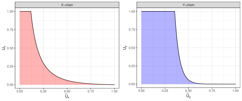
Figure 8: Illustration of acceptance mechanism for the $X$ and $Y$-chains in the $d\to\infty$ limit. Shaded regions correspond to $\tilde{B}_{x}=1$ and $\tilde{B}_{y}=1$, that is $U_{x}\leq f_{l}(\tilde{U}_{x};x)$ and $U_{y}\leq f_{l}(\tilde{U}_{y};y)$. The parameters are fixed at $(l,x,y)=(2.38,1,10)$, corresponding to optimal scaling for mixing at stationarity, the $X$-chain being stationary, and the $Y$-chain being in the tail of the target (away from the mode).

We construct this coupling sequentially. Let the full $d$-dimensional $X$-chain use random numbers $U_{x},Z_{x}^{(d)}$. Similarly define $U_{y},Z_{y}^{(d)}$ for the $Y$-chain. Let $Z\sim\mathcal{N}_{d}(0,I_{d})$ and $Z_{1},Z_{2}\sim\mathcal{N}(0,1)$ be independent of $U_{x,y},Z_{x,y}^{(d)}$. We let $Z_{x}^{(d)}=Z-(n_{x}^{\top}Z_{1})n_{x}-Z_{1}n_{x}$ and $Z_{y}^{(d)}=Z-(n_{y}^{\top}Z_{2})n_{y}-Z_{2}n_{y}$. This is similar to the easier-to-sample variant of the GCRN coupling, however we now let the coupling of $Z_{1},Z_{2}$ be arbitrary (but fixed for all $d$), instead of fixing $Z_{1}=Z_{2}$. This coupling ensures that $h^{2}Z_{x}^{(d)\top}Z_{y}^{(d)}\to l^{2}$ in $L_{2}$ as $d\to\infty$, and so under this coupling we have that

$$\lim_{d\to\infty}\mathbb{E}\left[\eqref{eqn:innerprod-cross}\mid\frac{\lVert X_{t}\rVert^{2}}{d}=x,\frac{\lVert Y_{t}\rVert^{2}}{d}=y,\frac{X_{t}^{\top}Y_{t}}{d}=v\right]=l^{2}\mathbb{E}[\tilde{B}_{x}\land\tilde{B}_{y}].$$

(Using again arguments similar to the proof of Theorem 2.)

We now define a coupling of $\tilde{B}_{x}$ and $\tilde{B}_{y}$ that ensures asymptotic optimality. Following the inverse-CDF method, let $Z_{1}=\Phi^{-1}(\tilde{U}_{x})$ and $Z_{2}=\Phi^{-1}(\tilde{U}_{y})$ where $\tilde{U}_{x},\tilde{U}_{y}\sim\textup{Unif}(0,1)$. Then,

$$\tilde{B}_{x}=\mathbbm{1}\big{\{}U_{x}\leq f(\tilde{U}_{x};x)\big{\}},\quad\tilde{B}_{y}=\mathbbm{1}\big{\{}U_{y}\leq f_{l}(\tilde{U}_{y};y)\big{\}},$$

where $f_{l}(\tilde{U};x)=e^{-lx^{1/2}\Phi^{-1}(\tilde{U})-l^{2}/2}$, $(U_{x},\tilde{U}_{x})\sim\otimes^{2}\textup{Unif}(0,1)$ and $(U_{y},\tilde{U}_{y})\sim\otimes^{2}\textup{Unif}(0,1)$.

To finish the construction of an asymptotically optimal Markovian coupling, we sample from a coupling of $\{(U_{x},\tilde{U}_{x}),(U_{y},\tilde{U}_{y})\}\sim\{\otimes^{2}\textup{Unif}(0,1),\otimes^{2}\textup{Unif}(0,1)\}$ such that as much mass is transported between the shaded regions of Figure 8 as possible. Under such a coupling, $\mathbb{E}[\tilde{B}_{x}\land\tilde{B}_{y}]=\mathbb{E}[\tilde{B}_{x}]\land\mathbb{E}[\tilde{B}_{y}]$, and so we have that

$$\lim_{d\to\infty}\mathbb{E}\left[\eqref{eqn:innerprod-cross}\mid\frac{\lVert X_{t}\rVert^{2}}{d}=x,\frac{\lVert Y_{t}\rVert^{2}}{d}=y,\frac{X_{t}^{\top}Y_{t}}{d}=v\right]=l^{2}\mathbb{E}[\tilde{B}_{x}]\land\mathbb{E}[\tilde{B}_{y}].$$

Therefore, the coupling is asymptotically optimal.

ODE limit under the asymptotically optimal Markovian coupling

Under an asymptotically optimal Markovian coupling, the ODE limit (IP) is recovered with $g(x,y,v)=g_{\textup{opt}}(x,y)$. By definition, no other coupling can obtain an ODE limit with faster convergence towards its limiting value.

Appendix D Computational details

All computations are carried out in (r). Code to reproduce the numerical experiments can be found at https://github.com/tamaspapp/rwmcouplings.

D.1 ODE limits

Let $(Z_{1},Z_{2})\sim\operatorname{BvN}(\rho)$ and define the bivariate normal probabilities $\operatorname{BvN}_{\textup{low}}(p,q;\rho)=\mathbb{P}(Z_{1}\leq p,Z_{2}\leq q)$ and $\operatorname{BvN}_{\textup{up}}(p,q;\rho)=\mathbb{P}(Z_{1}\geq p,Z_{2}\geq q)$.

We outline calculations carried out for the numerical computation of the ODE limit. We solve ODEs numerically using deSolve::ode (deSolve). The key term to evaluate is the integral

$$g(x,y,v)=\mathbb{E}\left[1\land e^{-lx^{1/2}Z_{1}-l^{2}/2}\land e^{-ly^{1/2}Z_{2}-l^{2}/2}\right]=\mathbb{E}\left[1\land e^{lx^{1/2}Z_{1}-l^{2}/2}\land e^{ly^{1/2}Z_{2}-l^{2}/2}\right].$$

To compute $g(x,y,v)$ under the CRN and reflection couplings, we rewrite this quantity in terms of numerically tractable quantities, see Lemma 9 below. We compute bivariate normal probabilities to machine precision using mvtnorm::pmvnorm (mvtnorm).

Lemma 9.

Suppose that $\rho\in(-1,1)$. Then,

$$g(x,y,v)=\operatorname{BvN}_{\textup{up}}(\frac{l}{2x^{1/2}},\frac{l}{2y^{1/2}};\rho)+h(x,y,\rho)+h(y,x,\rho),$$

where $h(x,y,\rho)=e^{l^{2}(x-1)/2}\operatorname{BvN}_{\textup{low}}(a/\sqrt{1+b^{2}},U;\rho=-b/\sqrt{1+b^{2}})$ with $b=-\{(x/y)^{1/2}-\rho\}/\sqrt{1-\rho^{2}}$, $a=blx^{1/2}$, $U=l/(2x^{1/2})-lx^{1/2}$.

Proof.

Suppose that $\rho\in(-1,1)$. Let $A=lx^{1/2}Z_{1}-l^{2}/2$, $B=ly^{1/2}Z_{2}-l^{2}/2$, such that $g(x,y,v)=\mathbb{E}\left[e^{0\land A\land B}\right]$. Split this expectation according to the partition $\{A,B\geq 0\}$, $\{A<0,A<B\}$, $\{B<0,B<A\}$, $\{A<0,A=B\}$, and then use that $\mathbb{P}(A=B)=0$ to obtain

$$g(x,y,v)= \mathbb{P}(A\geq 0,B\geq 0)+\mathbb{E}\mathbbm{1}_{\{A<0\}}\mathbbm{1}_{\{A<B\}}e^{A}+\mathbb{E}\mathbbm{1}_{\{B<0\}}\mathbbm{1}_{\{B<A\}}e^{B}$$

$$= \mathbb{P}(Z_{1}\geq\frac{l}{2x^{1/2}},Z_{2}\geq\frac{l}{2y^{1/2}})+h(x,y,\rho)+h(y,x,\rho)$$

$$= \operatorname{BvN}_{\textup{up}}(\frac{l}{2x^{1/2}},\frac{l}{2y^{1/2}},\rho)+h(x,y,\rho)+h(y,x,\rho),$$

where $h$ is defined as

$$h(x,y,\rho) =\mathbb{E}\mathbbm{1}_{\{lx^{1/2}Z_{1}<l^{2}/2\}}\mathbbm{1}_{\{lx^{1/2}Z_{1}<ly^{1/2}Z_{2}\}}e^{lx^{1/2}Z_{1}-l^{2}/2}.$$

We now express $h$ in terms of numerically tractable quantities. Expand $Z_{2}=\rho Z_{1}+\sqrt{1-\rho^{2}}Z_{*}$ where $Z_{*}\sim\mathcal{N}(0,1)$ is independent of $Z_{1}$. Integrate over the latter random variable to obtain $\mathbb{E}_{Z_{*}}\mathbbm{1}_{\{lx^{1/2}Z_{1}<ly^{1/2}Z_{2}\}}=\mathbb{P}_{Z_{*}}\big{(}(x/y)^{1/2}Z_{1}<\rho Z_{1}+\sqrt{1-\rho^{2}}Z_{*}\big{)}=\Phi(bZ_{1})$, where $b=-\{(x/y)^{1/2}-\rho\}/\sqrt{1-\rho^{2}}$. As such,

$$h(x,y,\rho)/e^{l^{2}(x-1)/2} =\mathbb{E}\mathbbm{1}_{\{Z_{1}<l/(2x^{1/2})\}}\Phi\left(bZ_{1}\right)e^{lx^{1/2}Z_{1}-l^{2}x/2}$$

$$=\int_{-\infty}^{l/(2x^{1/2})}\Phi(bz)e^{lx^{1/2}z-l^{2}x/2}\phi(z)\mathrm{d}z$$

$$=\int_{-\infty}^{l/(2x^{1/2})}\Phi(bz)\phi(z-lx^{1/2})\mathrm{d}z$$

$$=\int_{-\infty}^{l/(2x^{1/2})-lx^{1/2}}\Phi\big{(}b(z+lx^{1/2})\big{)}\phi(z)\mathrm{d}z$$

$$=\int_{-\infty}^{U}\Phi(a+bz)\phi(z)\mathrm{d}z=\operatorname{BvN}_{\textup{low}}(\frac{a}{\sqrt{1+b^{2}}},U;\rho=-\frac{b}{\sqrt{1+b^{2}}}),$$

where we have defined $a=blx^{1/2}$ and $U=l/(2x^{1/2})-lx^{1/2}$, we have used $e^{lx^{1/2}z-l^{2}x/2}\phi(z)=\phi(z-lx^{1/2})$ to obtain the fourth line, we have changed variables $z\leftarrow z-lx^{1/2}$ to obtain the fifth line, and finally we have used owen1980table. Substituting this expression into $g$ completes the proof. ∎

D.2 Elliptical Gaussian targets

AR(1) process

The covariance matrix $\Sigma_{d}$ of an AR(1) process with unit noise increments and correlation $\rho$ is a Kac-Murdock-Szegö matrix (see e.g. trench1999asymptotic). It holds that $\operatorname{tr}(\Sigma_{d})/d=1$ and $\lim_{d\to\infty}\operatorname{tr}(\Sigma_{d}^{-1})/d=(1+\rho^{2})/(1-\rho^{2})$.

Chi-square eigenvalues

The mean of a $\chi^{2}_{\nu}$ random variable is $\nu$, and the mean of an inverse chi-square random variable with the same degrees of freedom is $1/(\nu-2)$ provided that $\nu>2$. If the eigenvalues of the covariance $\Sigma_{d}$ are sampled from $\chi^{2}_{\nu}$, it thus holds that $\lim_{d\to\infty}\operatorname{tr}(\Sigma_{d})/d=\nu$ and $\lim_{d\to\infty}\operatorname{tr}(\Sigma_{d}^{-1})/d=1(\nu-2)$.

D.3 Stochastic volatility model

We consider the same stochastic volatility model as in (papp2022paper):

$$Y_{t}=\beta\varepsilon_{t}\exp\left(X_{t}/2\right),\quad\varepsilon_{t}\sim\mathcal{N}(0,1),\quad\textup{for }t=1,\dots,T,$$

$$X_{t+1}=\varphi X_{t}+\eta_{t+1},\quad\eta_{t+1}\sim\mathcal{N}(0,\sigma^{2}),\quad\textup{for }t=1,\dots,T-1,$$

$$X_{1}\sim\mathcal{N}\left(0,\sigma^{2}/(1-\varphi^{2})\right).$$

The log-posterior density $\pi(X_{1:T}\mid Y_{1:T})$ is, up to a constant offset,

$$\pi(X_{1:T}\mid Y_{1:T})=-\frac{1}{2}\left(\sum_{t=1}^{T}X_{t}+\frac{1}{\beta^{2}}\sum_{t=1}^{T}Y_{t}^{2}\exp(-X_{t})+\frac{1}{\sigma^{2}}\sum_{t=1}^{T-1}(\varphi X_{t}-X_{t+1})^{2}+\frac{1-\varphi^{2}}{\sigma^{2}}X_{1}^{2}\right).$$

The gradient of the log-posterior density $\nabla\log\pi(X_{1:T}\mid Y_{1:T})$ has components

$$\frac{\partial\pi}{\partial X_{1}} =-\frac{1}{2}+\frac{1}{2\beta^{2}}Y_{1}^{2}\exp(-X_{1})-\frac{\varphi}{\sigma^{2}}(\varphi X_{1}-X_{2})-\frac{1-\varphi^{2}}{\sigma^{2}}X_{1},$$

$$\frac{\partial\pi}{\partial X_{t}} =-\frac{1}{2}+\frac{1}{2\beta^{2}}Y_{t}^{2}\exp(-X_{t})-\frac{\varphi}{\sigma^{2}}(\varphi X_{t}-X_{t+1})-\frac{1}{\sigma^{2}}(X_{t}-\varphi X_{t-1}),\quad\textup{for }t=2,\dots T-1,$$

$$\frac{\partial\pi}{\partial X_{T}} =-\frac{1}{2}+\frac{1}{2\beta^{2}}Y_{T}^{2}\exp(-X_{T})-\frac{1}{\sigma^{2}}(X_{T}-\varphi X_{T-1}).$$

We fix the dimension $T=360$ and parameters $(\beta,\phi,\sigma)=(0.65,0.98,0.15)$. We simulate the data from the model; the data we use is slightly different to that used in (papp2022paper).

Appendix E Choice of threshold in RWM two-scale coupling

We investigate the choice of threshold $\delta$ in the two-scale coupling. We use $R=100$ pairs of coupled chains, a lag of $L=2\times 10^{6}$, and a step size $h=0.013$. As per Figure 9, the threshold $\delta=0.1$ appears to achieve the lowest average meeting time among the thresholds considered. The figure also indicates that overshooting the optimal threshold is perilous, and can lead to the distribution of meeting times having a relatively heavy tail. In contrast, underestimating the optimal threshold is much less problematic, maintaining the distribution of the meeting times similarly concentrated around its expectation and only slowly increasing this expectation.

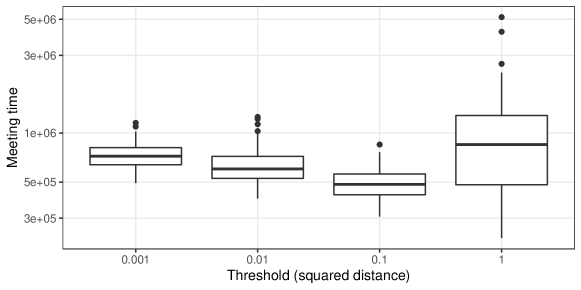
Figure 9: Threshold $\delta$ vs. meeting times for the two-scale RWM coupling on the SVM of Section 5.1. The smallest threshold of $\delta=0.001$ corresponds to a $2\%$ chance of coalesced proposals. For all other thresholds, this probability is negligibly small and $\leq 10^{-13}$.

We now put the threshold $\delta$ into context. Let the coupled proposals be $X_{p}\sim\mathcal{N}_{d}(X_{t},h^{2}I)$ and $Y_{p}\sim\mathcal{N}_{d}(Y_{t},h^{2}I)$. Under a maximal coupling, $\mathbb{P}(X_{p}=Y_{p})=2\Phi(-\lVert X_{t}-Y_{t}\rVert/(2h))=\mathbb{P}(\chi^{2}_{1}\geq\lVert X_{t}-Y_{t}\rVert^{2}/(4h^{2}))$, and so $\lVert X_{t}-Y_{t}\rVert^{2}$ uniquely determines the probability of the proposals coalescing. To have an $\mathbb{P}(X_{p}=Y_{p})=O(1)$ chance of coalescing the proposal, one needs to have $\lVert X_{t}-Y_{t}\rVert^{2}=O(h^{2})$.

To minimize the average meeting time under the two-scale coupling, one might now be tempted to choose the threshold $\delta$ (under which the reflection-maximal coupling is applied) such that $\delta=O(h^{2})$, and so there is always an $O(1)$ chance of coalescence whenever the reflection-maximal coupling is used. However, Figure 9 (where $h^{2}\approx 10^{-4}$) indicates that this is sub-optimal and instead a significantly larger scaling should be used for $\delta$.

The following heuristic suggests the choice $\delta=O(1)$ is optimal, and leads to $O(d)$ expected meeting times. In general, the optimal threshold $\delta$ will also depend on constants (target and step size parameters) which are not considered here, and so we recommend tuning $\delta$ by a grid search.

Optimality of $\delta=O(1)$

Pre-empting the discussion below, when $\delta\ll d^{1/2}$ and $\delta\gg h^{2}$ we claim that the behaviour of the two-scale coupling can be described as follows:

• Until $\delta$ in squared distance, due to the GCRN coupling the squared distance process behaves like an exponentially decaying ODE, decaying by a factor of $1-O(h^{2})$ at each iteration.

• Below $\delta$ in squared distance, due to the reflection coupling the distance process behaves like a symmetric random walk with increments $O(h)$. This random walk has a boundary at $0$ and a sticky boundary at $\delta^{1/2}$, where it typically spends $O(1/(h\delta^{1/2}))$ time before again jumping below $\delta^{1/2}$.

Following e.g. syed2022non-reversible, the expected time for the latter process to:

• make a trip from $\delta$ to $0$ is on the order of $\delta/h^{2}+1/(h\delta^{1/2})=(\delta+h\delta^{-1/2})/h^{2}$;

• make a round trip from $\delta$ to $0$ and back to $\delta$ is on the order of $\delta/h^{2}+(\delta^{1/2}/h)/(h\delta^{1/2})=(\delta+1)/h^{2}$.

The former is an expected hitting time. Once the chains are $O(h^{2})$ distance apart, there is an $O(1)$ chance of coalescence. The average meeting time is dependent on both the expected hitting and round-trip times.

Comparing the expected hitting and round-trip times to the $O(d)$ time for the two-scale coupling to reach $\delta$ from $O(d)$ suggests that the scaling $\delta=O(1)$ is optimal, striking a balance between the initial deterministic phase and the secondary stochastic phase. Decreasing $\delta$ increases the duration of the initial deterministic phase, while the round-trip time suggests that an $O(h^{2})=O(d)$ expected meeting time is unavoidable even if $\delta$ is chosen to decrease with $d$. Conversely, while increasing $\delta$ decreases the duration of the initial deterministic phase, the expected hitting and round-trip times increase strictly faster than $O(d)$ if $\delta$ is chosen to grow with $d$. This explanation is supported by the results of Figure 9.

Justifying the behaviour of two-scale coupling

We now justify the above description of the two-scale process. Suppose that the dimension $d$ is high, $\delta\ll d$, and $\delta\gg h^{2}$. Consider the process tracking the squared distance $\lVert Y_{t}-X_{t}\rVert^{2}$ between the chains, and suppose that it is started from $\delta$. Our goal is to bring the process to $O(h^{2})$ so that the chains can coalesce.

The GCRN coupling behaves nearly deterministically for this process, contracting the chains by an amount $1-O(h^{2})$ at each iteration. The time to reach $\delta$ from $O(d)$ is therefore on the order of $(1/h^{2})\log(d/\delta)=O(1/h^{2})=O(d)$ up to logarithmic terms in $d$. Similarly, under the GCRN coupling the time to reach $O(h^{2})$ from $\delta$ is on the order of $(1/h^{2})\log(\delta/h^{2})=\tilde{O}(1/h^{2})=\tilde{O}(d)$.

In contrast, a two-scale coupling has a random walk-like behaviour. Firstly, the reflection-maximal coupling essentially only reflects the proposals whenever $\lVert Y_{t}-X_{t}\rVert^{2}\gg h^{2}$, as then coupling essentially has a null chance of coalescing the proposals. Secondly, since the chains are quite close ($\lVert Y_{t}-X_{t}\rVert^{2}\leq\delta\ll d$) it holds that the reflection-coupled proposals are essentially only accepted or rejected simultaneously, since the projections of the noise increments $Z_{x},Z_{y}$ onto the normalized gradients $n_{x},n_{y}$ have a correlation of approximately $1$. Now, the distance between the proposals under the reflection coupling is $\lVert Y_{p}-X_{p}\rVert=\big{|}\lVert Y_{t}-X_{t}\rVert+2hZ_{\parallel}\big{|}\approx\lVert Y_{t}-X_{t}\rVert+2hZ_{\parallel}$ when $\lVert Y_{t}-X_{t}\rVert^{2}\gg h^{2}$, where $Z_{\parallel}\sim\mathcal{N}(0,1)$ is proportional to the component of $Z_{y}-Z_{x}$ parallel to $Y-X$. Due to the many degrees of freedom in dimension $d$, in the typical scenario $Z_{\parallel}$ is approximately independent to the projection of $Z_{x}$ onto $n_{x}$. Therefore, $\lVert Y_{p}-X_{p}\rVert$ is typically independent of the acceptance mechanism. After integrating over the acceptance random variables, we hence obtain that

$$\mathbb{E}_{\textup{acc}}\lVert Y_{t+1}-X_{t+1}\rVert\approx\lVert Y_{t}-X_{t}\rVert+chZ_{\parallel},$$ (19)

where $c>0$ is independent of the dimension.

Equation (19) indicates that the reflection-maximal coupling behaves like a symmetric random walk for the process $\lVert Y_{t}-X_{t}\rVert$, with jumps of size $O(h)$. When $\lVert Y_{t}-X_{t}\rVert$ overshoots $\delta^{1/2}$ by $h$, the GCRN coupling brings $\lVert Y_{t}-X_{t}\rVert$ back down to $\delta^{1/2}$ in $(1/h^{2})\log\{(\delta^{1/2}+h)/\delta^{1/2}\}=O(1/(h\delta^{1/2}))$ time. This can be interpreted as a “sticky” boundary condition at $\delta$ for the random walk, where there is an $O(h\delta^{1/2})$ probability of remaining at $\delta$, and otherwise an $O(h)$ jump below $\delta$ is performed.

Appendix F Bias of Laplace approximation

Define the mean and covariance of the SVM target $\mathbb{E}_{\pi}(X)=\mu$, $\textup{Var}_{\pi}(X)=\Sigma$, and similarly $\hat{\mu},\hat{\Sigma}$ for the Laplace approximation. According to the GCRN coupling and the lower bound gelbrich1990on, up to low Monte Carlo error it holds that

$$1.3\geq W_{2}^{2}(\pi,\hat{\pi})\geq W_{2}^{2}(\mathcal{N}(\mu,\Sigma),\mathcal{N}(\hat{\mu},\hat{\Sigma})).$$ (20)

Equation (20) contextualizes the error of the Laplace approximation in terms of the mean and covariance of the target. Suppose, for simplicity, that $\Sigma,\hat{\Sigma}$ commute. Then, $W_{2}^{2}(\mathcal{N}(\mu,\Sigma),\mathcal{N}(\hat{\mu},\hat{\Sigma}))=\lVert\mu-\hat{\mu}\rVert^{2}+\lVert\Sigma^{1/2}-\hat{\Sigma}^{1/2}\rVert_{F}^{2}$, where $\lVert\cdot\rVert_{F}$ is the Frobenius norm. The relevant scales of the Laplace approximation are $\lVert\hat{\mu}\rVert^{2}\approx 171$, $\lVert\hat{\Sigma}^{1/2}\rVert_{F}^{2}\approx 40$. We thus obtain the following approximate bounds on the relative error:

$$\lVert\mu-\hat{\mu}\rVert/\lVert\mu\rVert\leq 8.7\times 10^{-2},\quad\lVert\Sigma^{1/2}-\hat{\Sigma}^{1/2}\rVert_{F}/\lVert\Sigma^{1/2}\rVert_{F}\leq 1.8\times 10^{-1}.$$

Appendix G Coupling the Hug and Hop algorithm

We refer to ludkin2022hug for an algorithmic description of the Hug and Hop algorithm.

CRN Hug coupling

The CRN coupling samples the same initial momenta and uses the same uniform acceptance random variable for both chains. This coupling consistently contracts the chains in high dimension. For illustration, let the target be spherical Gaussian target $\pi=\mathcal{N}_{d}(0,I_{d})$, let the high dimension $d$ be high, and let only one bounce be performed ($B=1$). Hug always stays on the same level set when the target is spherical, so its acceptance rate is exactly 1. After one iteration,

$$X_{t+1} =X_{t}+\delta v-\frac{\delta X_{t}^{\top}v+\frac{\delta^{2}}{2}\lVert v\rVert^{2}}{\lVert X_{t}\rVert^{2}+\delta X_{t}^{\top}v+\frac{\delta^{2}}{4}\lVert v\rVert^{2}}(X_{t}+\frac{\delta}{2}v)$$

$$\approx(1-\frac{\frac{\delta^{2}}{2}\lVert v\rVert^{2}}{\lVert X_{t}\rVert^{2}+\frac{\delta^{2}}{4}\lVert v\rVert^{2}})X_{t}+\delta(1-\frac{\frac{\delta^{2}}{4}\lVert v\rVert^{2}}{\lVert X_{t}\rVert^{2}+\frac{\delta^{2}}{4}\lVert v\rVert^{2}})v,$$

whenever $\delta\gg d^{-1}$, since then $\delta\lVert v\rVert^{2}\approx\delta d\gg X_{t}^{\top}v=O(1)$. When the $X$-chain is stationary it approximately holds that that $\lVert X_{t}\rVert^{2}/d=\lVert v\rVert^{2}/d=1$, so

$$X_{t+1}\approx(1-\frac{2\delta^{2}}{4+\delta^{2}})X_{t}+\delta(1-\frac{\delta^{2}}{4+\delta^{2}})v.$$

Under a CRN coupling, when the $Y$-chain is stationary it similarly holds that

$$Y_{t+1}\approx(1-\frac{2\delta^{2}}{4+\delta^{2}})Y_{t}+\delta(1-\frac{\delta^{2}}{4+\delta^{2}})v,$$

such that $\lVert Y_{t+1}-X_{t+1}\lVert\approx(1-\frac{2\delta^{2}}{4+\delta^{2}})\lVert Y_{t}-X_{t}\lVert$. Therefore, the chains contract whenever $\delta\in(0,2)$.

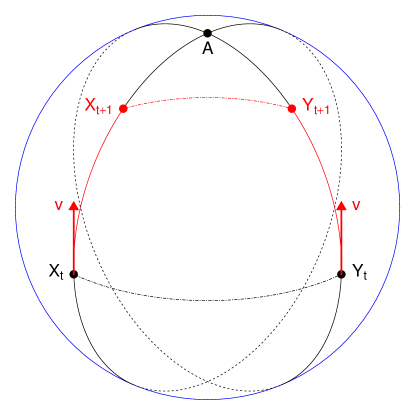
Figure 10: 3D visualisation of the contractive behaviour of CRN Hug in high dimension. While the pictured scenario has a relatively low probability of occurring in 3D, as the dimension increases the probability of occurrence approaches 1.

Our interpretation of this behaviour is as follows. For spherical targets, the level sets are (hyper)spheres, and the exact Hug dynamics move with constant speed along great circles. Assume that $X,Y$ are on the same level set and, for now, that the velocities at $X$ and $Y$ are chosen arbitrarily. In high dimension, the contribution of a small number of components in each velocity is negligible. Therefore, one can view the velocities at $X,Y$ to be orthogonal to the great circle containing $X,Y$. Hence, $X$ and $Y$ move along great circles which are orthogonal to the great circle containing $X,Y$. Now, start off the chains with the same velocity, which due to the high dimension can be viewed as being tangent to the level set at both $X,Y$. The contractive behaviour of this coupling is illustrated in Figure 10. Measured in great-circle distance, the two paths are farthest away at $(X,Y)$. Due to the synchronous velocity, the chains move towards the point of intersection $A$ of the great circles (or its antipode) at the same speed, and so the chains must contract irrespective of the time the dynamics are run for.

This intuition extends to elliptical targets by replacing the level sets by (hyper)ellipsoids, and so on. Experiments with high-dimensional elliptical targets (not pictured) confirm that the contractivity of finely discretized Hug chains under the CRN coupling is insensitive to the length of the integration time.

Threshold in two-scale Hop coupling

One might expect the GCRN coupling to contract Hop proposals, however it does not allow for exact meetings irrespective of the number of iterations it is run for. In contrast, the maximal coupling allows for the chains to meet exactly with positive probability at each iteration, but otherwise tends to expand the proposals. Varying the threshold $\delta$ trades off between these two behaviours. We investigate the choice of $\delta$, finding that the the average meeting times increase rapidly as $\delta$ is increased beyond the optimum of $\delta=10^{-4}$, but increase much slowly below the optimum (see Figure 11; we use $R=100$ pairs of coupled chains and a lag of $L=6\times 10^{3}$). This confirms that the GCRN coupling contracts the Hop chains, and that the contraction is key to obtaining meeting times which are representative of the convergence of the Hug and Hop algorithm.

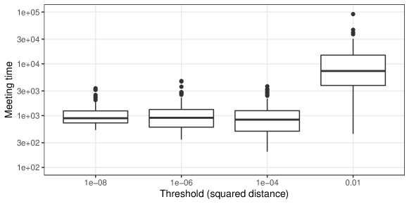
Figure 11: Threshold $\delta$ vs. meeting times for the two-scale Hug and Hop coupling on the SVM of Section 5.1.

Poor performance of CRN Hop coupling

We replaced the GCRN coupling with a CRN coupling in the two-scale Hop kernel. Running 10 pilot pairs of chains each for $10^{5}$ iterations, we found that only one pair met (after $\approx 4\times 10^{4}$ iterations). This outlines the importance of the GCRN coupling in contracting the chains. The following explains the poor performance of the CRN coupling. The Hop analogue of term (5) drives the contraction of the chains under a given coupling. As for the RWM, the acceptance mechanism for Hop is dominated by the gradient direction. In addition, the scaling is much larger in the gradient direction for Hop than for the RWM, so the term $(X_{p}-X)^{\top}(Y_{p}-Y)$ has a larger contribution from the gradient. Therefore, any discrepancy between the projections onto gradient directions leads to a larger “expanding” effect for Hop than for the RWM.

Appendix H The 3D process is Markov in the standard Gaussian case

Suppose that the target is standard Gaussian $\pi=\mathcal{N}(0,I_{d})$. We assume that $\lVert X_{t}\rVert,\lVert Y_{t}\rVert\neq 0$; dealing with the case when one or both are null is straightforward and the proof is omitted. Let $\widehat{X}_{t}=X_{t}/\lVert X_{t}\rVert$ and $\widehat{Y}_{t}=Y_{t}/\lVert Y_{t}\rVert$.

In order to show that $(W_{t})_{t\geq 0}$ is Markov, it is sufficient to show that $\{(\lVert X_{t}\rVert^{2},\lVert Y_{t}\rVert^{2},X_{t}^{\top}Y_{t})\}_{t\geq 0}$ is Markov. We have the following expressions, shared by all three couplings:

$$\lVert X_{t+1}\rVert^{2} =\lVert X_{t}\rVert^{2} +(2h\lVert X_{t}\rVert\widehat{X}_{t}^{\top}Z_{x}+h^{2}\lVert Z_{x}\rVert^{2})\mathbbm{1}\{U\leq e^{-h\lVert X_{t}\rVert\widehat{X}_{t}^{\top}Z_{x}-h^{2}\lVert Z_{x}\rVert^{2}/2}\},$$

$$\lVert Y_{t+1}\rVert^{2} =\lVert Y_{t}\rVert^{2} +(2h\lVert Y_{t}\rVert\widehat{Y}_{t}^{\top}Z_{y}+h^{2}\lVert Z_{y}\rVert^{2})\mathbbm{1}\{U\leq e^{-h\lVert Y_{t}\rVert\widehat{Y}_{t}^{\top}Z_{y}-h^{2}\lVert Z_{y}\rVert^{2}/2}\},$$

$$X_{t+1}^{\top}Y_{t+1} =X_{t}^{\top}Y_{t} +h\lVert Y_{t}\rVert\widehat{Y}_{t}^{\top}Z_{x}\mathbbm{1}\{U\leq e^{-h\lVert X_{t}\rVert\widehat{X}_{t}^{\top}Z_{x}-h^{2}\lVert Z_{x}\rVert^{2}/2}\}$$

$$+h\lVert X_{t}\rVert\widehat{X}_{t}^{\top}Z_{y}\mathbbm{1}\{U\leq e^{-h\lVert Y_{t}\rVert\widehat{Y}_{t}^{\top}Z_{y}-h^{2}\lVert Z_{y}\rVert^{2}/2}\}$$

$$+h^{2}Z_{x}^{\top}Z_{y}\mathbbm{1}\{U\leq e^{(-h\lVert X_{t}\rVert\widehat{X}_{t}^{\top}Z_{x}-h^{2}\lVert Z_{x}\rVert^{2}/2)\land(-h\lVert Y_{t}\rVert\widehat{Y}_{t}^{\top}Z_{y}-h^{2}\lVert Z_{y}\rVert^{2}/2)}\}.$$

Showing that the process $\{(\lVert X_{t}\rVert^{2},\lVert Y_{t}\rVert^{2},X_{t}^{\top}Y_{t})\}_{t\geq 0}$ is Markov thus reduces to showing that the joint distribution of $(\widehat{X}_{t}^{\top}Z_{x},\widehat{Y}_{t}^{\top}Z_{x},\widehat{X}_{t}^{\top}Z_{y},\widehat{Y}_{t}^{\top}Z_{y},\lVert Z_{x}\rVert^{2},\lVert Z_{y}\rVert^{2})$ is uniquely determined by the triplet $(\lVert X_{t}\rVert^{2},\lVert Y_{t}\rVert^{2},X_{t}^{\top}Y_{t})$. Consider the projections of $Z_{x},Z_{y}$ onto $\textup{span}\{X_{t},Y_{t}\}$ and its orthogonal complement separately. The joint randomness reduces to a $\chi^{2}_{d-2}$ random variable and, independently, a 6-D multivariate normal with zero mean and a covariance matrix that is uniquely determined by $(\lVert X_{t}\rVert^{2},\lVert Y_{t}\rVert^{2},X_{t}^{\top}Y_{t})$, and so it follows that the process of interest is Markov. The calculations themselves are straightforward, but tedious, and are omitted.

Fast simulation of high-dimensional chains

Our process of interest has a three-dimensional state space irrespective of the underlying $d$-dimensional state space the marginal chains are supported on. Since the low-dimensional process is Markov, one can directly simulate it, which yields a large reduction in computational cost (when the dimension $d$ is large) compared to simulating the coupled pair of chains $\{(X_{t},Y_{t})\}_{t\geq 0}$, where each chain has a $d$-dimensional state.

We do not pursue this route, as the simulation of the full chains is numerically tractable in the scenarios we consider.

References

- Beskos et al. (2013) Alexandros Beskos, Natesh Pillai, Gareth Roberts, Jesus-Maria Sanz-Serna, and Andrew Stuart. Optimal tuning of the hybrid Monte Carlo algorithm. Bernoulli, 19(5A):1501 – 1534, 2013. doi: 10.3150/12-BEJ414. URL https://doi.org/10.3150/12-BEJ414.
- Biswas and Mackey (2021) Niloy Biswas and Lester Mackey. Bounding Wasserstein distance with couplings. arXiv preprint arxiv:2112.03152, 2021. URL https://arxiv.org/abs/2112.03152.
- Biswas et al. (2019) Niloy Biswas, Pierre E. Jacob, and Paul Vanetti. Estimating convergence of Markov chains with L-lag couplings. In Advances in Neural Information Processing Systems, volume 32, pages 7391–7401, 2019. URL https://papers.nips.cc/paper/2019/hash/aec851e565646f6835e915293381e20a-Abstract.html.
- Biswas et al. (2022) Niloy Biswas, Anirban Bhattacharya, Pierre E. Jacob, and James E. Johndrow. Coupling-based convergence assessment of some Gibbs samplers for high-dimensional Bayesian regression with shrinkage priors. Journal of the Royal Statistical Society: Series B (Statistical Methodology), 84(3):973–996, 2022. doi: https://doi.org/10.1111/rssb.12495. URL https://rss.onlinelibrary.wiley.com/doi/abs/10.1111/rssb.12495.
- Bou-Rabee et al. (2020) Nawaf Bou-Rabee, Andreas Eberle, and Raphael Zimmer. Coupling and convergence for Hamiltonian Monte Carlo. The Annals of Applied Probability, 30(3):1209 – 1250, 2020. URL https://doi.org/10.1214/19-AAP1528.
- Chen et al. (2020) Yuansi Chen, Raaz Dwivedi, Martin J. Wainwright, and Bin Yu. Fast mixing of metropolized hamiltonian monte carlo: Benefits of multi-step gradients. Journal of Machine Learning Research, 21(92):1–72, 2020. URL http://jmlr.org/papers/v21/19-441.html.
- Christensen et al. (2005) Ole F. Christensen, Gareth O. Roberts, and Jeffrey S. Rosenthal. Scaling limits for the transient phase of local Metropolis–Hastings algorithms. JRSS:B, 67(2):253–268, 2005. doi: 10.1111/j.1467-9868.2005.00500.x. URL https://doi.org/10.1111/j.1467-9868.2005.00500.x.
- Douc et al. (2022) Randal Douc, Pierre E. Jacob, Anthony Lee, and Dootika Vats. Solving the poisson equation using coupled markov chains, 2022. URL https://arxiv.org/abs/2206.05691.
- Duane et al. (1987) Simon Duane, A.D. Kennedy, Brian J. Pendleton, and Duncan Roweth. Hybrid monte carlo. Physics Letters B, 195(2):216–222, 1987. ISSN 0370-2693. doi: https://doi.org/10.1016/0370-2693(87)91197-X. URL https://www.sciencedirect.com/science/article/pii/037026938791197X.
- Durmus and Moulines (2019) Alain Durmus and Éric Moulines. High-dimensional Bayesian inference via the unadjusted Langevin algorithm. Bernoulli, 25(4A):2854–2882, 2019. URL https://doi.org/10.3150/18-BEJ1073.
- Eberle (2014) Andreas Eberle. Error bounds for Metropolis–Hastings algorithms applied to perturbations of Gaussian measures in high dimensions. The Annals of Applied Probability, 24(1):337–377, 2014. URL https://doi.org/10.1214/13-AAP926.
- Hairer et al. (2011) Martin Hairer, Jonathan C. Mattingly, and Michael Scheutzow. Asymptotic coupling and a general form of Harris’ theorem with applications to stochastic delay equations. Probability Theory and Related Fields, 149(1):223 – 259, 2011. doi: 10.1007/s00440-009-0250-6. URL https://doi.org/10.1007/s00440-009-0250-6.
- Heng and Jacob (2019) J Heng and P E Jacob. Unbiased Hamiltonian Monte Carlo with couplings. Biometrika, 106(2):287–302, 2019. URL https://doi.org/10.1093/biomet/asy074.
- Jacob et al. (2020) Pierre E. Jacob, John O’Leary, and Yves F. Atchadé. Unbiased Markov chain Monte Carlo methods with couplings. Journal of the Royal Statistical Society: Series B (Statistical Methodology), 82(3):543–600, 2020. URL https://doi.org/10.1111/rssb.12336.
- Liu (2001) Jun S. Liu. Monte Carlo Strategies in Scientific Computing. Springer, 2001.
- Ludkin and Sherlock (2022) M Ludkin and C Sherlock. Hug and Hop: a discrete-time, nonreversible Markov chain Monte Carlo algorithm. Biometrika, 07 2022. ISSN 1464-3510. doi: 10.1093/biomet/asac039. URL https://doi.org/10.1093/biomet/asac039. asac039.
- Mangoubi and Smith (2017) Oren Mangoubi and Aaron Smith. Rapid mixing of Hamiltonian monte carlo on strongly log-concave distributions, 2017. URL https://arxiv.org/abs/1708.07114.
- Middleton et al. (2020) Lawrence Middleton, George Deligiannidis, Arnaud Doucet, and Pierre E. Jacob. Unbiased Markov chain Monte Carlo for intractable target distributions. Electronic Journal of Statistics, 14(2):2842 – 2891, 2020. doi: 10.1214/20-EJS1727. URL https://doi.org/10.1214/20-EJS1727.
- Neal (2011) Radford M. Neal. MCMC Using Hamiltonian Dynamics, chapter 5. CRC Press, 2011. doi: 10.1201/b10905-7. URL https://doi.org/10.1201/b10905-7.
- Nguyen et al. (2022) Tin D. Nguyen, Brian L. Trippe, and Tamara Broderick. Many processors, little time: Mcmc for partitions via optimal transport couplings. In Gustau Camps-Valls, Francisco J. R. Ruiz, and Isabel Valera, editors, Proceedings of The 25th International Conference on Artificial Intelligence and Statistics, volume 151 of Proceedings of Machine Learning Research, pages 3483–3514. PMLR, 28–30 Mar 2022. URL https://proceedings.mlr.press/v151/nguyen22a.html.
- O’Leary (2021) John O’Leary. Couplings of the random-walk metropolis algorithm, 2021. URL https://arxiv.org/abs/2102.01790.
- O’Leary and Wang (2022) John O’Leary and Guanyang Wang. Metropolis-hastings transition kernel couplings. arXiv preprint arxiv:2102.00366, 2022. URL https://arxiv.org/abs/2102.00366.
- O’Leary et al. (2021) John O’Leary, Guanyang Wang, and Pierre Jacob. Maximal couplings of the metropolis-hastings algorithm. In Arindam Banerjee and Kenji Fukumizu, editors, Proceedings of The 24th International Conference on Artificial Intelligence and Statistics, volume 130 of Proceedings of Machine Learning Research, pages 1225–1233. PMLR, 13–15 Apr 2021. URL https://proceedings.mlr.press/v130/wang21d.html.
- Papp and Sherlock (2022) Tamás P. Papp and Chris Sherlock. Bounds on Wasserstein distances between continuous distributions using independent samples. arXiv::2203.11627 [stat.ML], 2022. URL https://arxiv.org/abs/2203.11627.
- R Core Team (2020) R Core Team. R: A Language and Environment for Statistical Computing. R Foundation for Statistical Computing, Vienna, Austria, 2020. URL https://www.R-project.org/.
- Roberts and Rosenthal (1998) Gareth O. Roberts and Jeffrey S. Rosenthal. Optimal scaling of discrete approximations to Langevin diffusions. Journal of the Royal Statistical Society: Series B (Statistical Methodology), 60(1):255–268, 1998. URL https://doi.org/10.1111/1467-9868.00123.
- Roberts and Rosenthal (2001) Gareth O. Roberts and Jeffrey S. Rosenthal. Optimal scaling for various Metropolis-Hastings algorithms. Statistical Science, 16(4):351 – 367, 2001. doi: 10.1214/ss/1015346320. URL https://doi.org/10.1214/ss/1015346320.
- Roberts and Rosenthal (2004) Gareth O. Roberts and Jeffrey S. Rosenthal. General state space Markov chains and MCMC algorithms. Probability Surveys, 1:20–71, 2004. URL https://doi.org/10.1214/154957804100000024.
- Roberts et al. (1997) Gareth O. Roberts, Andrew Gelman, and Walter R. Gilks. Weak convergence and optimal scaling of random walk Metropolis algorithms. The Annals of Applied Probability, 7(1):110–120, 1997. URL https://doi.org/10.1214/aoap/1034625254.
- Ruiz et al. (2021) Francisco J. R. Ruiz, Michalis K. Titsias, Taylan Cemgil, and Arnaud Doucet. Unbiased gradient estimation for variational auto-encoders using coupled Markov chains. In Proceedings of the Thirty-Seventh Conference on Uncertainty in Artificial Intelligence, volume 161 of Proceedings of Machine Learning Research, pages 707–717. PMLR, 2021. URL https://proceedings.mlr.press/v161/ruiz21a.html.
- Sherlock (2013) Chris Sherlock. Optimal scaling of the random walk Metropolis: general criteria for the 0.234 acceptance rule. Journal of Applied Probability, 50(1):1 – 15, 2013. doi: 10.1239/jap/1363784420. URL https://doi.org/10.1239/jap/1363784420.
- Sherlock and Roberts (2009) Chris Sherlock and Gareth Roberts. Optimal scaling of the random walk Metropolis on elliptically symmetric unimodal targets. Bernoulli, 15(3):774 – 798, 2009. doi: 10.3150/08-BEJ176. URL https://doi.org/10.3150/08-BEJ176.
- Thorisson (2000) Hermann Thorisson. Coupling, Stationarity, and Regeneration. Springer, 2000.
- Wang and Wang (2022) Guanyang Wang and Tianze Wang. Unbiased multilevel monte carlo methods for intractable distributions: Mlmc meets mcmc, 2022. URL https://arxiv.org/abs/2204.04808.

References

- Christensen et al. (2005) Ole F. Christensen, Gareth O. Roberts, and Jeffrey S. Rosenthal. Scaling limits for the transient phase of local Metropolis–Hastings algorithms. JRSS:B, 67(2):253–268, 2005. doi: 10.1111/j.1467-9868.2005.00500.x. URL https://doi.org/10.1111/j.1467-9868.2005.00500.x.
- Gelbrich (1990) Matthias Gelbrich. On a formula for the L2 Wasserstein metric between measures on Euclidean and Hilbert spaces. Mathematische Nachrichten, 147(1):185–203, 1990. URL https://doi.org/10.1002/mana.19901470121.
- Genz et al. (2021) Alan Genz, Frank Bretz, Tetsuhisa Miwa, Xuefei Mi, Friedrich Leisch, Fabian Scheipl, and Torsten Hothorn. mvtnorm: Multivariate Normal and t Distributions, 2021. URL https://CRAN.R-project.org/package=mvtnorm. R package version 1.1-3.
- Kallenberg (2021) Olav Kallenberg. Foundations of Modern Probability. Springer, 2021. URL https://doi.org/10.1007/978-3-030-61871-1.
- Ludkin and Sherlock (2022) M Ludkin and C Sherlock. Hug and Hop: a discrete-time, nonreversible Markov chain Monte Carlo algorithm. Biometrika, 07 2022. ISSN 1464-3510. doi: 10.1093/biomet/asac039. URL https://doi.org/10.1093/biomet/asac039. asac039.
- Owen (1980) Donald Bruce Owen. A table of normal integrals. Communications in Statistics - Simulation and Computation, 9(4):389–419, 1980. doi: 10.1080/03610918008812164. URL https://doi.org/10.1080/03610918008812164.
- Papp and Sherlock (2022) Tamás P. Papp and Chris Sherlock. Bounds on Wasserstein distances between continuous distributions using independent samples. arXiv::2203.11627 [stat.ML], 2022. URL https://arxiv.org/abs/2203.11627.
- R Core Team (2020) R Core Team. R: A Language and Environment for Statistical Computing. R Foundation for Statistical Computing, Vienna, Austria, 2020. URL https://www.R-project.org/.
- Roberts et al. (1997) Gareth O. Roberts, Andrew Gelman, and Walter R. Gilks. Weak convergence and optimal scaling of random walk Metropolis algorithms. The Annals of Applied Probability, 7(1):110–120, 1997. URL https://doi.org/10.1214/aoap/1034625254.
- Sato (1999) Ken-iti Sato. Lévy Processes and Infinitely Divisible Distributions. Cambridge Studies in Advanced Mathematics. Cambridge University Press, 1999. ISBN 9780521553025.
- Soetaert et al. (2010) Karline Soetaert, Thomas Petzoldt, and R. Woodrow Setzer. Solving differential equations in R: Package deSolve. Journal of Statistical Software, 33(9):1–25, 2010. doi: 10.18637/jss.v033.i09.
- Syed et al. (2022) Saifuddin Syed, Alexandre Bouchard-Côté, George Deligiannidis, and Arnaud Doucet. Non-reversible parallel tempering: A scalable highly parallel mcmc scheme. Journal of the Royal Statistical Society: Series B (Statistical Methodology), 84(2):321–350, 2022. doi: https://doi.org/10.1111/rssb.12464. URL https://rss.onlinelibrary.wiley.com/doi/abs/10.1111/rssb.12464.
- Trench (1999) William F. Trench. Asymptotic distribution of the spectra of a class of generalized Kac–Murdock–Szegö matrices. Linear Algebra and its Applications, 294(1):181–192, 1999. URL https://doi.org/10.1016/S0024-3795(99)00080-4.
- Villani (2003) Cédric Villani. Topics in Optimal Transportation. Graduate studies in mathematics. American Mathematical Society, 2003. URL http://doi.org/10.1090/gsm/058.
- Øksendal (1998) Bernt Øksendal. Stochastic Differential Equations. Springer-Verlag, 5 edition, 1998. URL https://doi.org/10.1007/978-3-662-03620-4.