A Study of Warm Dark Matter, the Missing Satellites Problem, and the UV Luminosity Cut-Off

Abstract

In the warm dark matter scenario, the Press-Schechter formalism is valid only for galaxy masses greater than the “velocity dispersion cut-off". In this work we extend the predictions to masses below the velocity dispersion cut-off, and thereby address the “Missing Satellites Problem", and the rest-frame ultra-violet luminosity cut-off required to not exceed the measured reionization optical depth. We find agreement between predictions and observations of these two phenomena. As a by-product, we obtain the empirical Tully-Fisher relation from first principles.

1 Introduction

Two apparent problems with the cold dark matter $\Lambda$CDM cosmology are the “Missing Satellites Problem", and the need of a rest-frame ultra-violet (UV) luminosity cut-off. The “Missing Satellites Problem" is the reduced number of observed Local Group satellites compared to the number obtained in $\Lambda$CDM simulations (Klypin, 1999). A UV luminosity cut-off is needed to not exceed the reionization optical depth $\tau=0.054\pm 0.007$ measured by the Planck collaboration (Planck, 2018) (Workman, 2022) (Lapi, 2015) (Mason, 2015). In the present study we consider warm dark matter as a possible solution to both problems.

The Press-Schechter formalism, when applied to warm dark matter, includes the free-streaming cut-off, but not the “velocity dispersion cut-off", and is therefore only valid for total (dark matter plus baryon) linear perturbation masses $M$ greater than the velocity dispersion cut-off mass $M_{\textrm{vd}}$ (to be explained below). The purpose of the present study is to extend the Press-Schechter prediction to $M<M_{\textrm{vd}}$, and compare this extension with the “Missing Satellites Problem", and with the needed UV luminosity cut-off.

We continue the study of warm dark matter presented in Hoeneisen (2022c). Our point of departure is Figure 1 of Hoeneisen (2022c). Here we reproduce the panel corresponding to redshift $z=6$ in Figure 1 (with one change: instead of the Gaussian window function in Hoeneisen (2022c), in the present article we use the sharp-$k$ window function throughout, with mass parameter $c=1.555$ as explained in Hoeneisen (2022c)). Figure 1 compares distributions, i.e. numbers of galaxies per decade (dex) and per Mpc³, of galaxy linear total (dark matter plus baryon) perturbation masses $M$, stellar masses $M_{*}$, and rest-frame ultra-violet (UV) luminosities $\nu L_{UV}$, with the Press-Schechter prediction (Press-Schechter, 1974), and its Sheth-Tormen ellipsoidal collapse extensions with parameter $\nu\equiv 1.686/\sigma$ (not to be confused with the frequency above) and $0.84\nu$ (Sheth-Tormen, 1999) (Sheth-Mo-Tormen, 2001). The data on $M_{*}$ is obtained from Lapi (2017), Song (2016), Grazian (2015), and Davidzon (2017). The data on $\nu L_{UV}$, where $\nu$ is the frequency corresponding to wavelength $1550$Å, is obtained from Lapi (2015), Bouwens (2015), Bouwens (2021), and McLeod (2015). The UV luminosities have been corrected for dust extinction as described in Lapi (2015) and Bouwens (2014). The predictions depend on the warm dark matter free-streaming comoving cut-off wavenumber $k_{\textrm{fs}}(t_{\textrm{eq}})$, and the comparisons of predictions with data provide a measurement of $k_{\textrm{fs}}(t_{\textrm{eq}})$, see Hoeneisen (2022c) for full details. In Figure 1 the predictions extend down to the velocity dispersion cut-offs indicated by red, blue and green dots (Hoeneisen, 2022c) (Hoeneisen, 2022b). The purpose of the present study is to extend the predictions to smaller $M_{*}$ and $\nu L_{\textrm{UV}}$, and thereby address the “Missing Satellites Problem", and the UV luminosities cut-off, respectively.

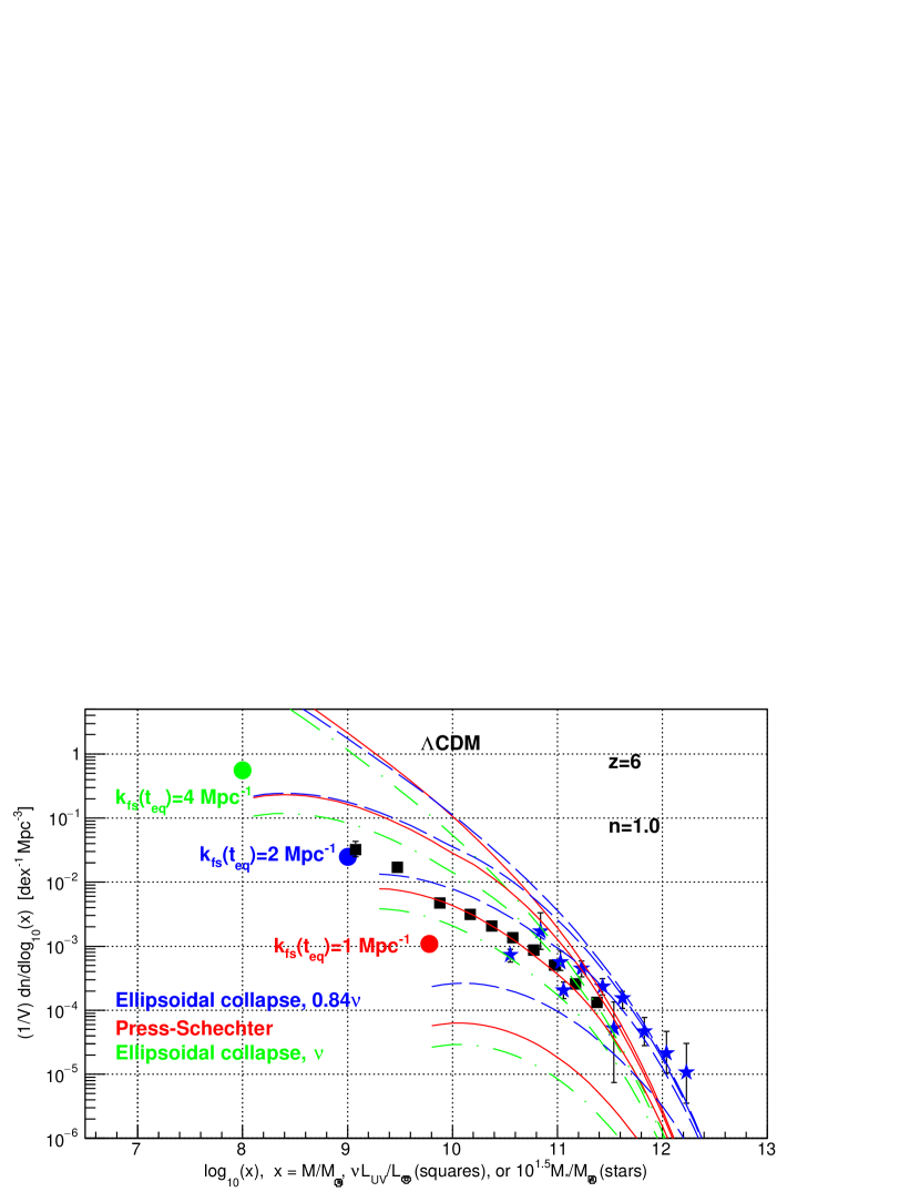
Figure 1: Shown are distributions of $x$, where $x$ is the observed galaxy stellar mass $M_{*}/M_{\odot}$ times $10^{1.5}$ (stars) (Lapi, 2017) (Song, 2016) (Grazian, 2015) (Davidzon, 2017), or the observed galaxy UV luminosity $\nu L_{\textrm{UV}}/L_{\odot}$ (squares) (Lapi, 2015) (Bouwens, 2015) (Bouwens, 2021) (McLeod, 2015) (corrected for dust extinction (Lapi, 2015) (Bouwens, 2014)), or the predicted linear total (dark matter plus baryon) perturbation mass $M/M_{\odot}$ (lines), at redshift $z=6$. The Press-Schechter prediction, and its Sheth-Tormen ellipsoidal collapse extensions, correspond, from top to bottom, to the warm dark matter free-streaming cut-off wavenumbers $k_{\textrm{fs}}(t_{\textrm{eq}})=1000,4,2$ and $1$ Mpc^-1. The round red, blue and green dots indicate the velocity dispersion cut-offs of the predictions (Hoeneisen, 2022b) at $k_{\textrm{fs}}(t_{\textrm{eq}})=1,2$ and 4 Mpc^-1, respectively. Presenting three predictions illustrates the uncertainty of the predictions.

2 Velocity Dispersion and Free-Streaming

To obtain a self-contained article, we need to define the warm dark matter adiabatic invariant $v_{h\textrm{rms}}(1)$, and the free-streaming cut-off factor $\tau^{2}(k)$, as in Hoeneisen (2022c). We consider non-relativistic warm dark matter to be a clasical (non-degenerate) gas of particles, as justified in Paduroiu (2015) and Hoeneisen (2022a). Let $v_{h\textrm{rms}}(a)$ be the root-mean-square velocity of non-relativistic warm dark matter particles in the early universe at expansion parameter $a$. As the universe expands it cools, so $v_{h\textrm{rms}}(a)$ decreases in proportion to $a^{-1}$ (if dark matter collisions, if any, do not excite particle internal degrees of freedom (Hoeneisen, 2022d)). Therefore,

$$v_{h\textrm{rms}}(1)=v_{h\textrm{rms}}(a)a=v_{h\textrm{rms}}(a)\left[\frac{\Omega_{c}\rho_{\textrm{crit}}}{\rho_{h}(a)}\right]^{1/3},$$ (1)

is an adiabatic invariant. $\rho_{h}(a)=\Omega_{c}\rho_{\textrm{crit}}/a^{3}$ is the dark matter density. The warm dark matter velocity dispersion causes free-streaming of dark matter particles in and out of density minimums and maximums, and so attenuates the power spectrum of relative density perturbations $(\rho(\mathbf{x})-\bar{\rho})/\bar{\rho}$ of the cold dark matter $\Lambda$CDM cosmology by a factor $\tau^{2}(k)$. $k$ is the comoving wavenumber of relative density perturbations. At the time $t_{\textrm{eq}}$ of equal radiation and matter densities, $\tau^{2}(k)$ has the approximate form (Boyanovsky, 2008)

$$\tau^{2}(k)\approx\exp{\left[-k^{2}/k^{2}_{\textrm{fs}}(t_{\textrm{eq}})\right]},$$ (2)

where the comoving cut-off wavenumber, due to free-streaming, is (Boyanovsky, 2008)

$$k_{\textrm{fs}}(t_{\textrm{eq}})=\frac{1.455}{\sqrt{2}}\sqrt{\frac{4\pi G\bar{\rho}_{h}(1)a_{\textrm{eq}}}{v_{h\textrm{rms}}(1)^{2}}}.$$ (3)

After $t_{\textrm{eq}}$, the Jeans mass decreases as $a^{-3/2}$, so $\tau^{2}(k)$ develops a non-linear regenerated “tail" when the relative density perturbations approach unity (White, 2018). We will take $\tau^{2}(k)$, at the time of galaxy formation, to have the form

$$\tau^{2}(k) = \exp{\left(-\frac{k^{2}}{k^{2}_{\textrm{fs}}(t_{\textrm{eq}})}\right)}\qquad\textrm{ if }k<k_{\textrm{fs}}(t_{\textrm{eq}}),$$ (4)

$$= \exp{\left(-\frac{k^{n}}{k^{n}_{\textrm{fs}}(t_{\textrm{eq}})}\right)}\qquad\textrm{ if }k\geq k_{\textrm{fs}}(t_{\textrm{eq}}).$$

The parameter $n$ allows a study of the effect of the non-linear regenerated tail. If $n=2$, there is no regenerated tail. Agreement between the data and predictions, down to the velocity dispersion cut-off dots in Figure 1, is obtained with $n$ in the approximate range 1.1 to 0.2 (Hoeneisen, 2022c).

A comment: In (4) we should have written $k_{\textrm{fs}}(t_{\textrm{gal}})$ instead of $k_{\textrm{fs}}(t_{\textrm{eq}})$, where $t_{\textrm{gal}}$ is the time of galaxy formation. However, the measurement $k_{\textrm{fs}}(t_{\textrm{gal}})=2.0^{+0.8}_{-0.5}\textrm{ Mpc}^{-1}$ with galaxy UV luminosity distributions and galaxy stellar mass distributions (Hoeneisen, 2022c), is in agreement with the measurement of $k_{\textrm{fs}}(t_{\textrm{eq}})=1.90\pm 0.32\textrm{ Mpc}^{-1}$ with dwarf galaxy rotation curves (from the measurement of the adiabatic invariant $v_{h\textrm{rms}}(1)=0.406\pm 0.069$ km/s in Hoeneisen (2022d), and Equation (3)). So we do not distinguish $k_{\textrm{fs}}(t_{\textrm{gal}})$ from $k_{\textrm{fs}}(t_{\textrm{eq}})$ (until observations require otherwise).

Let us now consider the velocity dispersion cut-off. In the $\Lambda$CDM scenario, when a spherically symmetric relative density perturbation $(\rho(\mathbf{x})-\bar{\rho})/\bar{\rho}$ reaches 1.686 in the linear approximation, the exact solution diverges, and a galaxy forms. This is the basis of the Press-Schechter formalism. The same is true in the warm dark matter scenario if the linear total (dark matter plus baryon) perturbation mass $M$ exceeds the velocity dispersion cut-off $M_{\textrm{vd0}}$. For $M<M_{\textrm{vd0}}$, the galaxy formation redshift $z$ is delayed by $\Delta z$ due to the velocity dispersion. This delay $\Delta z$ is not included in the Press-Schechter formalism. $\Delta z$ is obtained by numerical integration of the galaxy formation hydro-dynamical equations, see Hoeneisen (2022b). The velocity dispersion cut-off mass $M_{\textrm{vd}}$, indicated by the dots in Figure 1, corresponds, by definition, to $\Delta z=1$. The values of $M_{\textrm{vd}}$ are presented in Hoeneisen (2022c). For $M>M_{\textrm{vd0}}=10^{0.67}M_{\textrm{vd}}$ we take $\Delta z=0$. For $M<M_{\textrm{vd0}}=10^{0.67}M_{\textrm{vd}}$ we may approximate $\Delta z\approx 1.5\left[\log_{10}(M_{\textrm{vd}}/M_{\odot})+0.67-\log_{10}(M/M_{\odot})\right]$. The values of $\log_{10}(M_{\textrm{vd}}/M_{\odot})$ are summarized in Table 1.

Table 1: The warm dark matter velocity dispersion delays the galaxy formation redshift $z$ by $\Delta z\approx 1.5\left[\log_{10}(M_{\textrm{vd}}/M_{\odot})+0.67-\log_{10}(M/M_{\odot})\right]$ if $M<M_{\textrm{vd0}}=10^{0.67}M_{\textrm{vd}}$. The values of $\log_{10}(M_{\textrm{vd}}/M_{\odot})$ are presented as a function of the galaxy formation redshift $z$, and the adiabatic invariant $v_{h\textrm{rms}}(1)$. $M_{\textrm{vd}}$ is obtained from numerical integrations of galaxy formation hydro-dynamical equations (Hoeneisen, 2022b). Also shown is $k_{\textrm{fs}}(t_{\textrm{eq}})$ form (3). By definition, at $M=M_{\textrm{vd}}$, $\Delta z=1.0$.

$z$	$v_{h\textrm{rms}}(1)$	$k_{\textrm{fs}}(t_{\textrm{eq}})$	$\log_{10}(M_{\textrm{vd}}/M_{\odot})$
4	0.75 km/s	1 Mpc-1	9.3
4	0.49 km/s	1.53 Mpc-1	8.5
4	0.37 km/s	2 Mpc-1	8.3
4	0.19 km/s	4 Mpc-1	7.5
6	0.75 km/s	1 Mpc-1	9.8
6	0.49 km/s	1.53 Mpc-1	9.3
6	0.37 km/s	2 Mpc-1	9.0
6	0.19 km/s	4 Mpc-1	8.0
8	0.75 km/s	1 Mpc-1	10.3
8	0.49 km/s	1.53 Mpc-1	9.6
8	0.37 km/s	2 Mpc-1	9.2
8	0.19 km/s	4 Mpc-1	8.2

3 Extending the Predictions to $M<M_{\textrm{vd0}}$

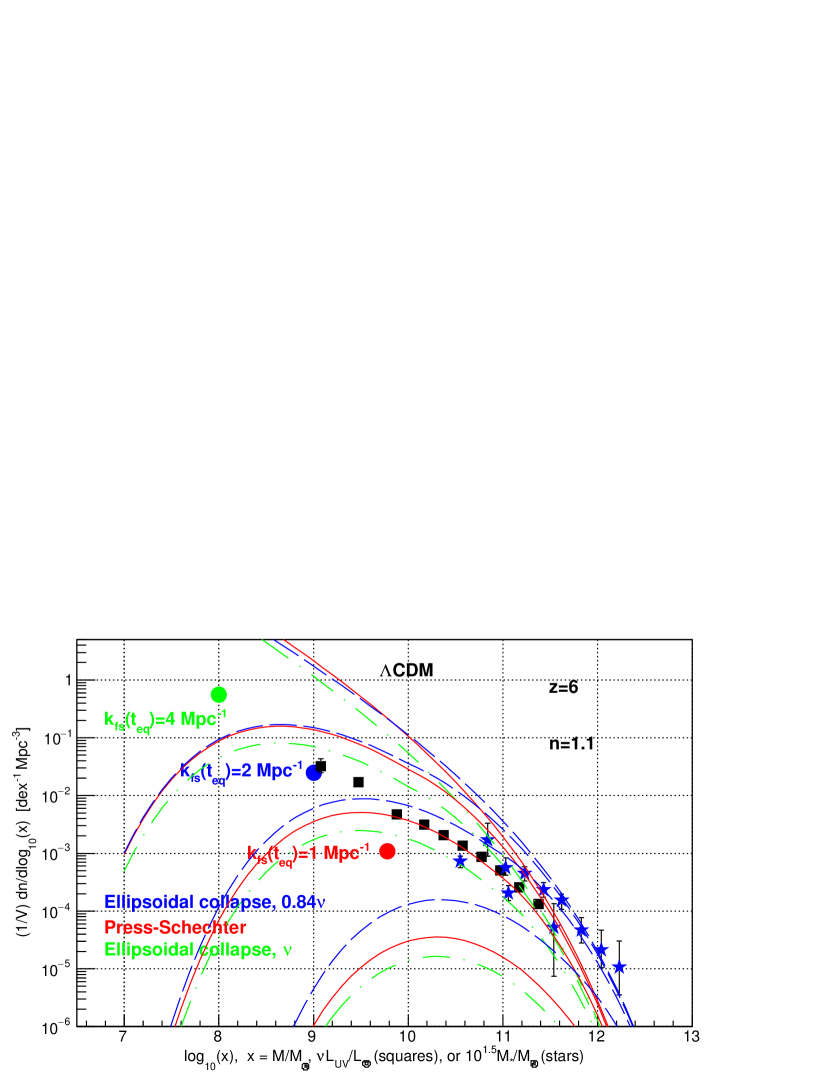
Figure 2: Same as Figure 1, i.e. $z=6$, but the predictions are extended to $M<M_{\textrm{vd}0}$ with the free-streaming cut-off with $\tau^{2}(k)$ with a tail with $n=2.0,1.1,0.7$ or 0.5, without the velocity dispersion cut-off.

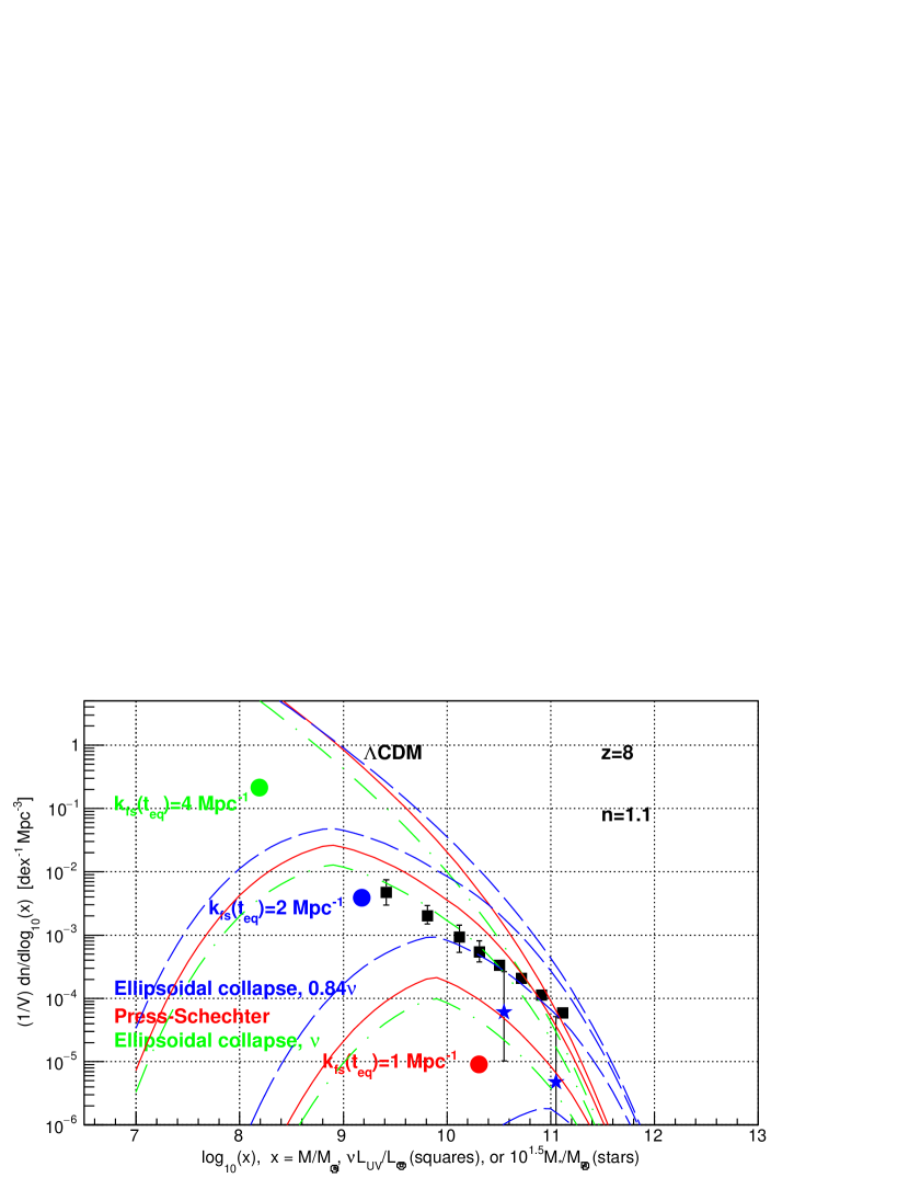
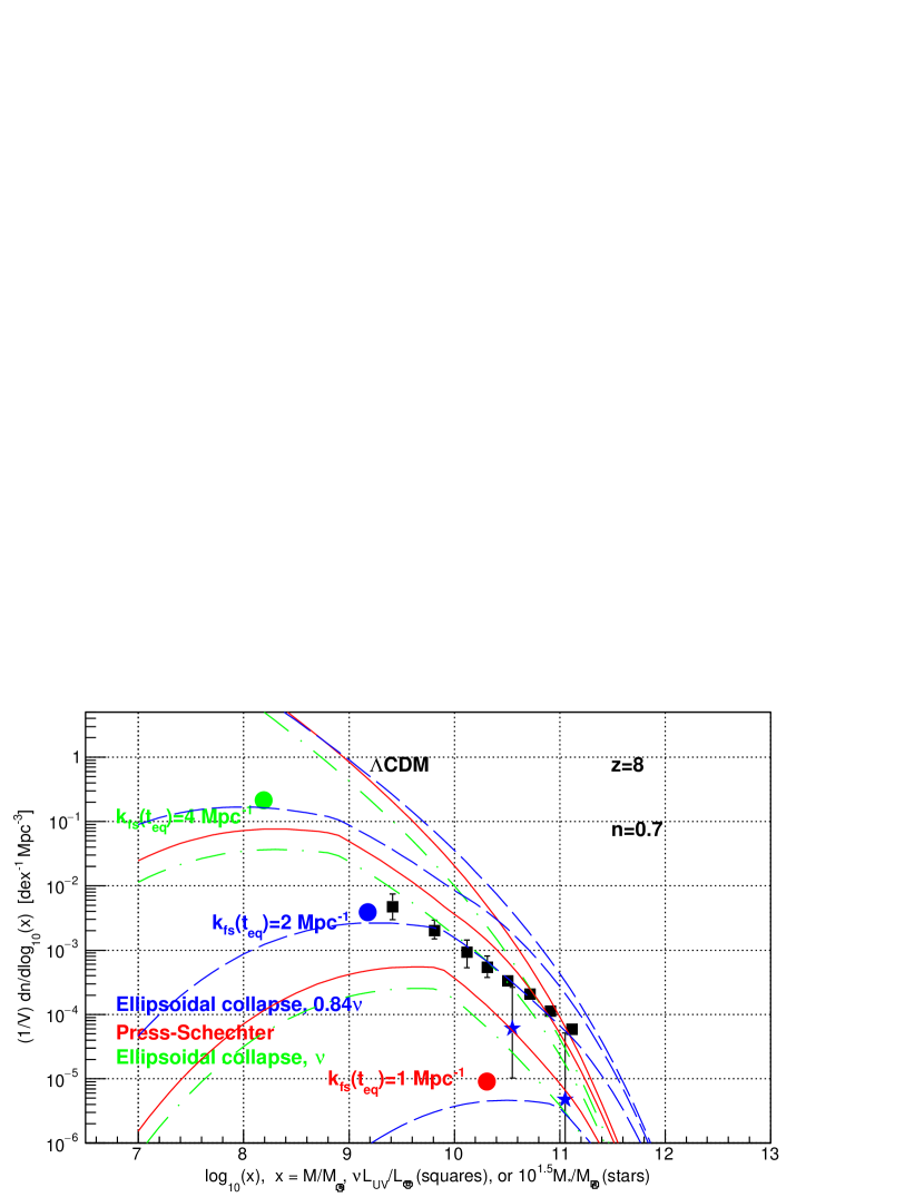
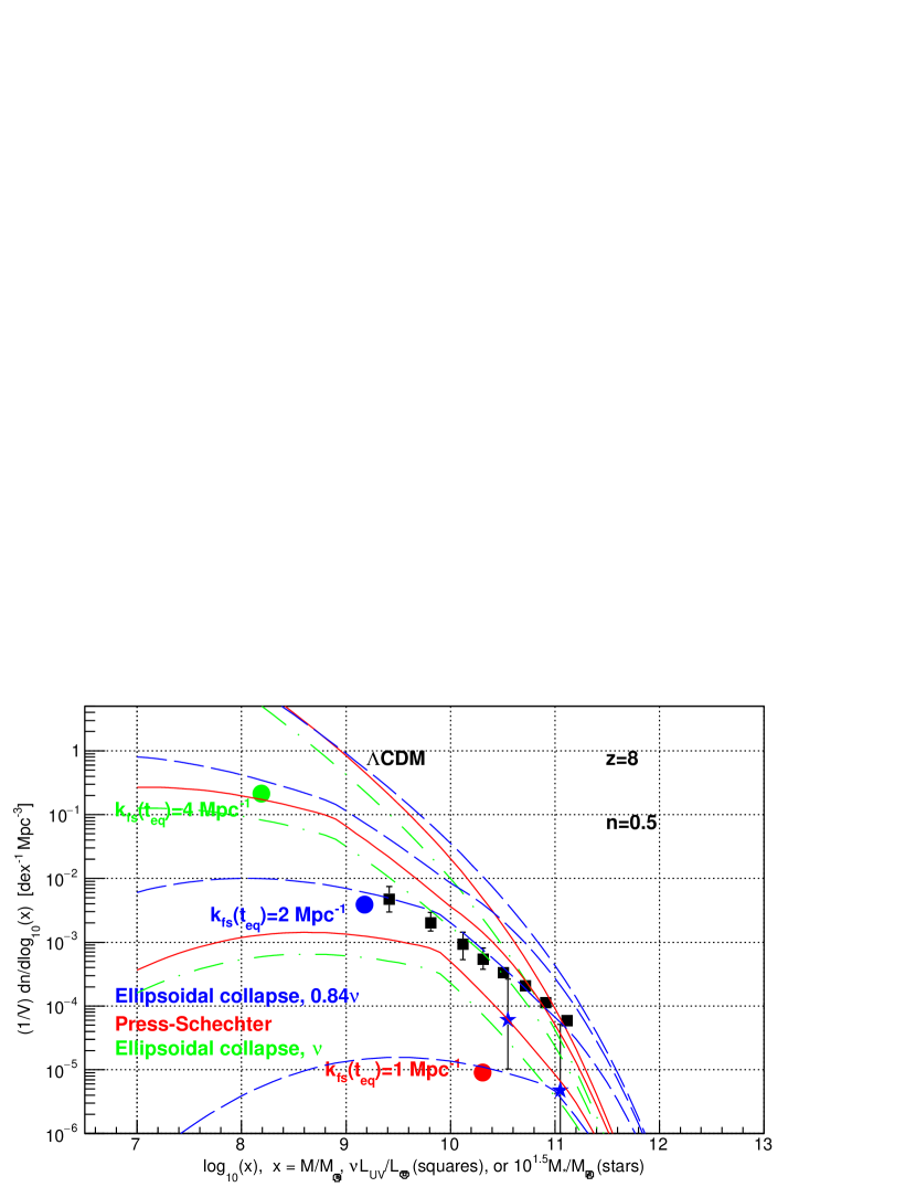
Figure 3: Predictions for $z=8$, and (from top to bottom) $k_{\textrm{fs}}(t_{\textrm{eq}})=1000,4,2,1\textrm{ Mpc}^{-1}$, are extended to $M<M_{\textrm{vd}0}$ with the free-streaming cut-off with $\tau^{2}(k)$ with a tail with $n=1.1,0.7,0.5$,or 0.3, and with the velocity dispersion cut-off. Agreement between predictions and observations are obtained with $k_{\textrm{fs}}(t_{\textrm{eq}})\approx 2\textrm{ Mpc}^{-1}$, and $0.8\gtrsim n\gtrsim 0.3$.

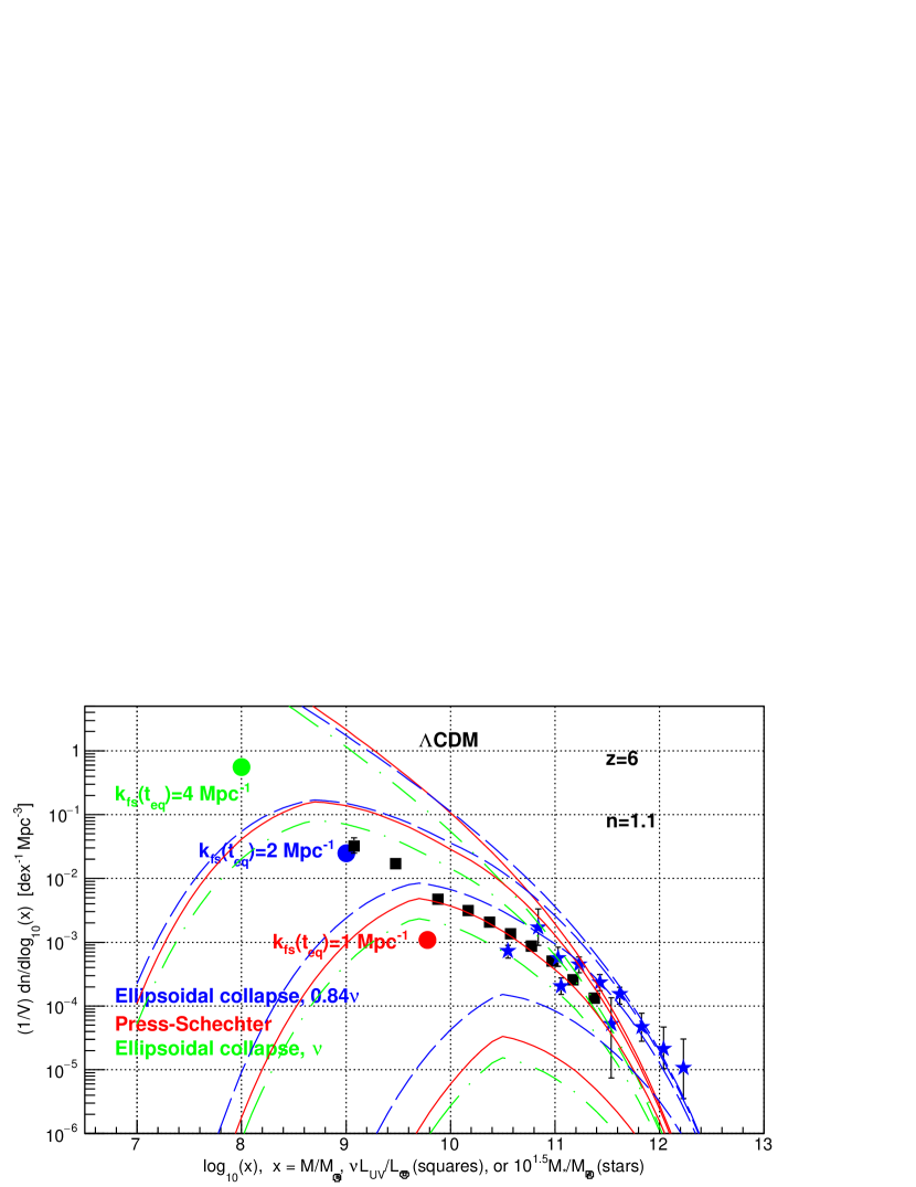
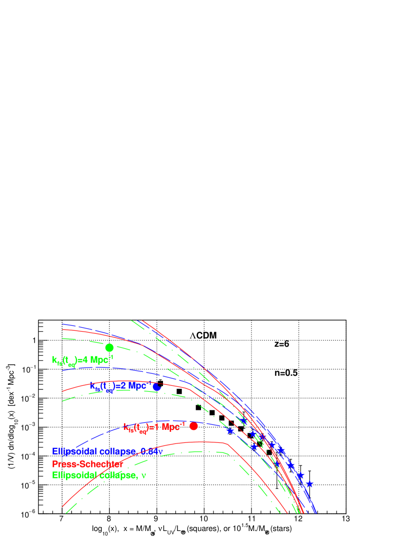
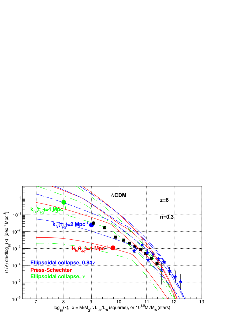
Figure 4: Predictions for $z=6$, and (from top to bottom) $k_{\textrm{fs}}(t_{\textrm{eq}})=1000,4,2,1\textrm{ Mpc}^{-1}$, are extended to $M<M_{\textrm{vd}0}$ with the free-streaming cut-off with $\tau^{2}(k)$ with a tail with $n=1.1,0.7,0.5$, or 0.3, and with the velocity dispersion cut-off. Agreement between predictions and observations are obtained with $k_{\textrm{fs}}(t_{\textrm{eq}})\approx 2\textrm{ Mpc}^{-1}$, and $0.8\gtrsim n\gtrsim 0.3$.

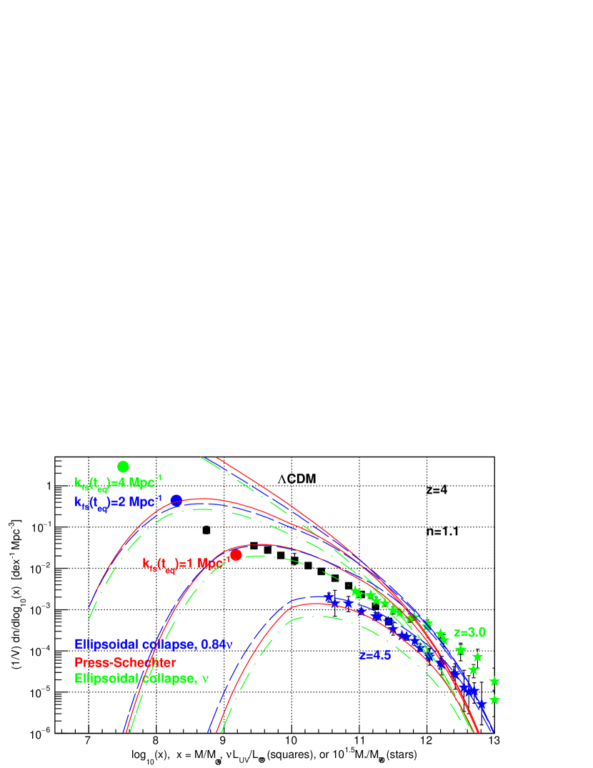
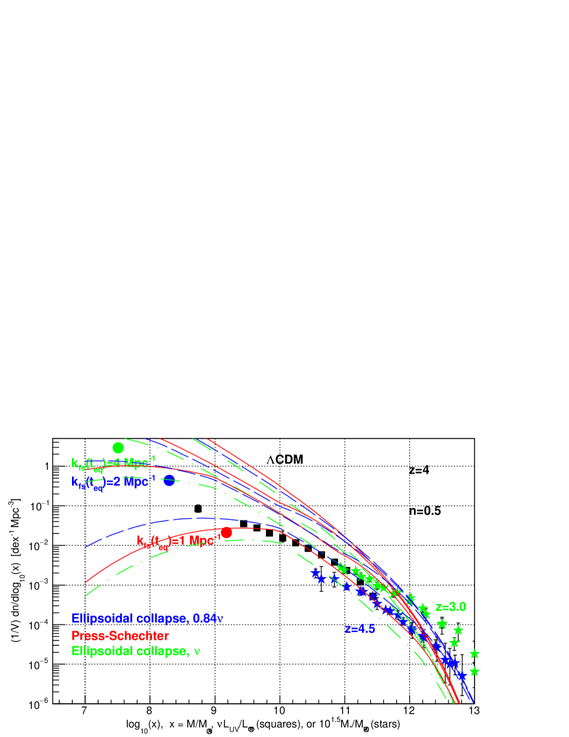
Figure 5: Predictions for $z=4$, and (from top to bottom) $k_{\textrm{fs}}(t_{\textrm{eq}})=1000,4,2,1\textrm{ Mpc}^{-1}$, are extended to $M<M_{\textrm{vd}0}$ with the free-streaming cut-off with $\tau^{2}(k)$ with a tail with $n=1.1,0.7,0.5$, or 0.3, and with the velocity dispersion cut-off. Agreement between predictions and observations are obtained with $k_{\textrm{fs}}(t_{\textrm{eq}})\approx 1.5\textrm{ Mpc}^{-1}$ and $n\approx 0.7$, or $k_{\textrm{fs}}(t_{\textrm{eq}})\approx 1\textrm{ Mpc}^{-1}$ and $n\approx 0.5$.

The Press-Schechter prediction, and its extensions, are based on the variance $\sigma^{2}(M,z,k_{\textrm{fs}}(t_{\textrm{eq}}),n)$ of the linear relative density perturbation $(\rho(\mathbf{x})-\bar{\rho})/\bar{\rho}$ at the total (dark matter plus baryon) mass scale $M$ (Hoeneisen, 2022c) (Weinberg, 2008). This variance depends on the redshift $z$ of galaxy formation, and on the parameters $k_{\textrm{fs}}(t_{\textrm{eq}})$ and $n$ of the free-streaming cut-off factor $\tau^{2}(k)$ of (4). Comparison of predictions and data for $M>M_{\textrm{vd0}}$ obtain a measurement of $k_{\textrm{fs}}(t_{\textrm{eq}})$, see Figure 1, and Hoeneisen (2022c). The extension of the predictions to $M<M_{\textrm{vd0}}$ depends on two cut-offs: the free-streaming cut-off (through the parameters $k_{\textrm{fs}}(t_{\textrm{eq}})=2.0^{+0.8}_{-0.5}\textrm{ Mpc}^{-1}$, that is already fixed by the measurements in Hoeneisen (2022c), and $n$), and the velocity dispersion cut-off. We illustrate the effect of $n$ in Figure 2, without applying the velocity dispersion cut-off yet. The velocity dispersion cut-off is implemented by replacing $\sigma^{2}(M,z,k_{\textrm{fs}}(t_{\textrm{eq}}),n)$ by $\sigma^{2}(M,z+\Delta z,k_{\textrm{fs}}(t_{\textrm{eq}}),n)$, with $\Delta z$ obtained from Table 1. We illustrate the effect of both $n$, and the velocity dispersion cut-off, in Figures 3, 4, and 5, for galaxy formation at $z=8,6$, and 4, respectively.

4 The Relation Between $M$ and $V_{\textrm{flat}}$

Table 2: The galaxy flat rotation velocity $V_{\textrm{flat}}$ [km/s] is presented as a function of the adiabatic invariant $v_{h\textrm{rms}}(1)$, and the galaxy formation redshift $z$, for linear perturbations of total (dark matter plus baryon) mass $M=2\times 10^{10}M_{\odot}$. Also shown is the free-streaming cut-off wavenumber $k_{\textrm{fs}}(t_{\textrm{eq}})$ from (3). $V_{\textrm{flat}}$ is obtained from numerical integration of galaxy formation hydro-dynamical equations (Hoeneisen, 2022b).

$v_{h\textrm{rms}}(1)$ [m/s]	750	490	370	190	0.75
$k_{\textrm{fs}}(t_{\textrm{eq}})$ [Mpc-1]	1	1.53	2	4	1000
$z$
4	38	33	36	37	34
5	41	35	37	37	37
6	47	44	40	49	42
8	45	42	45	46	49
10	51	49	47	53	51

Table 3: Shown are linear perturbation total (dark matter plus baryon) masses $M$, and the corresponding flat rotation velocities $V_{\textrm{flat}}$. These relations are approximately valid for galaxy formation at redshift $z$ between 6 and 10, and free-streaming cut-off wavenumber $k_{\textrm{fs}}(t_{\textrm{eq}})$ between 1 and 1000 Mpc^-1.

$M$	$V_{\textrm{flat}}$
$3\times 10^{12}M_{\odot}$	255 km/s
$1\times 10^{12}M_{\odot}$	188 km/s
$1\times 10^{11}M_{\odot}$	82 km/s
$5\times 10^{10}M_{\odot}$	71 km/s
$2\times 10^{10}M_{\odot}$	45 km/s
$1\times 10^{10}M_{\odot}$	37 km/s
$5\times 10^{9}M_{\odot}$	28 km/s
$3\times 10^{8}M_{\odot}$	9 km/s

The linear perturbation total (dark matter plus baryon) mass scale $M$, of the Press-Schechter formalism, can not be measured directly. We find that the flat portion of the rotation velocity of test particles in spiral galaxies, $V_{\textrm{flat}}$, can be used as an approximate proxy for $M$.

Given $M$, the galaxy formation redshift $z$, and $v_{h\textrm{rms}}(1)$, it is possible to obtain $V_{\textrm{flat}}$ by numerical integration of the galaxy formation hydro-dynamical equations (Hoeneisen, 2022b). Results for $M=2\times 10^{10}M_{\odot}$ are presented in Table 2. We note that for galaxy formation at redshift $z$ between 6 and 10, and free-streaming cut-off wavenumber $k_{\textrm{fs}}(t_{\textrm{eq}})$ between 1 and 1000 Mpc^-1, we may approximate $V_{\textrm{flat}}\approx 45$ km/s. Similarly, for several masses $M$, the corresponding rotation velocities $V_{\textrm{flat}}$ are summarized in Table 3. The data in Table 3 can be fit by the relation

$$\frac{M}{M_{\odot}}\approx 2.1\times 10^{8}\left(\frac{V_{\textrm{flat}}}{10\textrm{ km/s}}\right)^{3},$$ (5)

as shown in Figure 6. This becomes the Tully-Fisher relation, once $M/M_{\odot}$ is replaced by $\approx 10^{1.5}M_{*}/M_{\odot}\approx 10^{1.5}L_{*}/L_{\odot}$, see Figure 1:

$$\frac{L_{*}}{L_{\odot}}\approx 2.4\times 10^{10}h^{-2}\left(\frac{V_{\textrm{flat}}}{200\textrm{ km/s}}\right)^{3},$$ (6)

with $h=0.674$. $L_{*}$ is the stellar luminosity. It is very satisfactory to obtain quantitatively the empirical Tully-Fisher relation from the galaxy formation hydro-dynamical equations (Hoeneisen, 2022b), i.e. from first principles.

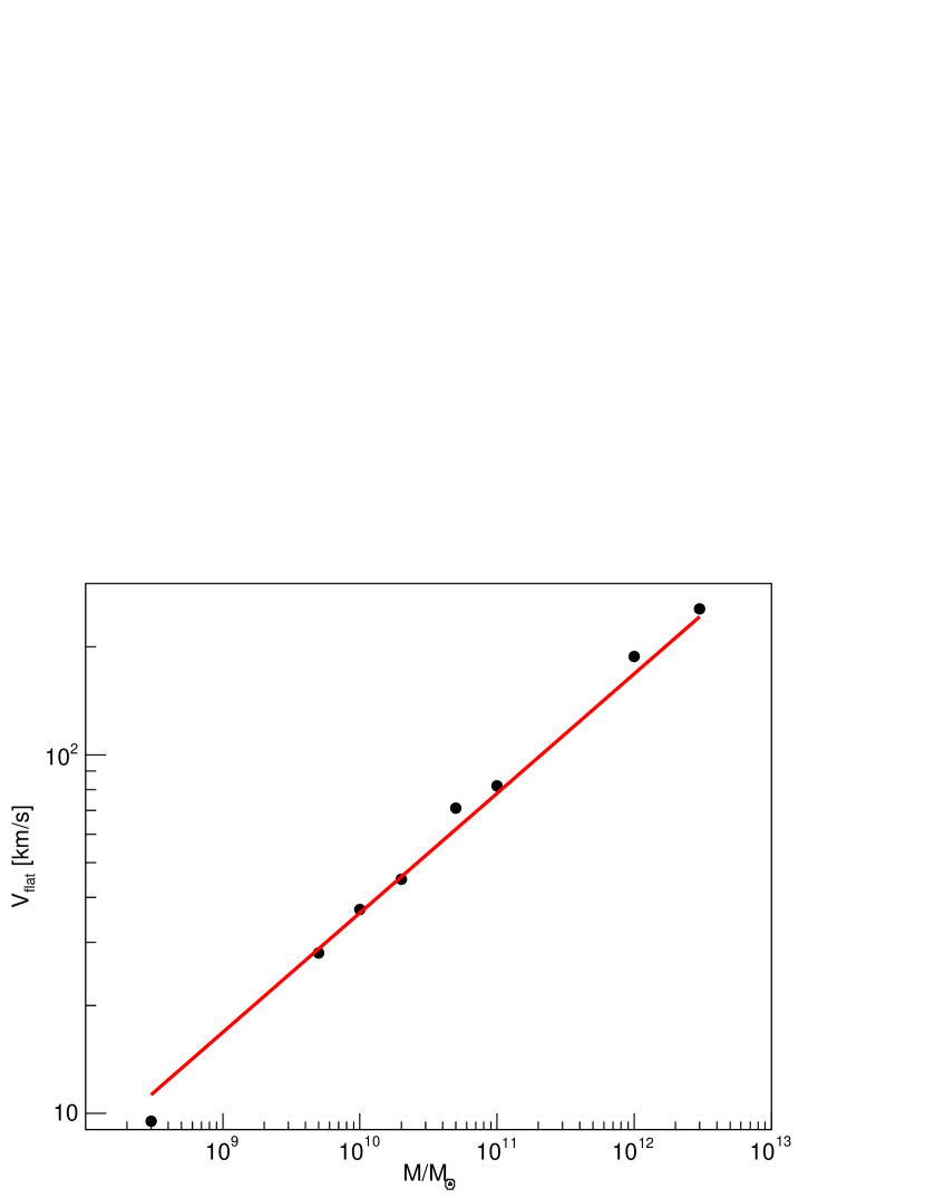
Figure 6: Presented is $V_{\textrm{flat}}$, from Table 3, as a function of the linear total (dark matter plus baryon) perturbation mass $M$, valid for galaxy formation at redshift $z$ between 6 and 10, and free-streaming cut-off wavenumber $k_{\textrm{fs}}(t_{\textrm{eq}})$ between 1 and 1000 Mpc^-1. The line is $M/M_{\odot}=2.1\times 10^{8}(V_{\textrm{flat}}/10\textrm{ km/s})^{3}$.

5 The “Missing Satellites Problem"

The “Missing Satellites Problem" is described in Klypin (1999). The approximate number of observed satellites within $200h^{-1}$ kpc of the Local Group, per Mpc³, with $V_{\textrm{flat}}>V$ is (Klypin, 1999)

$$n_{\textrm{obs}}(V_{\textrm{flat}}>V)\approx 385h^{3}\left(\frac{10\textrm{ km/s}}{V}\right)^{1.3}\textrm{ Mpc}^{-3},$$ (7)

while the corresponding number in the $\Lambda$CDM simulations is (Klypin, 1999)

$$n_{\textrm{sim}}(V_{\textrm{flat}}>V)\approx 5000h^{3}\left(\frac{10\textrm{ km/s}}{V}\right)^{2.75}\textrm{ Mpc}^{-3}.$$ (8)

Using (5), we find that the appropriate ratio to compare the $\Lambda$CDM simulation with observations is

$$\frac{dn_{\textrm{sim}}/dV_{\textrm{flat}}}{dn_{\textrm{obs}}/dV_{\textrm{flat}}}\approx\frac{5000\cdot 2.75}{385\cdot 1.3}\left(\frac{10\textrm{ km/s}}{V_{\textrm{flat}}}\right)^{1.45}.$$ (9)

Similarly, for satellites within $400h^{-1}$ kpc of the Local Group, the ratio is

$$\frac{dn_{\textrm{sim}}/dV_{\textrm{flat}}}{dn_{\textrm{obs}}/dV_{\textrm{flat}}}\approx\frac{1200\cdot 2.75}{55\cdot 1.4}\left(\frac{10\textrm{ km/s}}{V_{\textrm{flat}}}\right)^{1.35}.$$ (10)

We take agreement between observations and simulations at $V_{\textrm{flat}}\approx 70$ km/s, corresponding to $M\approx 10^{10.9}M_{\odot}$, see (5). We take $(dn_{\textrm{sim}}/dV_{\textrm{flat}})/(dn_{\textrm{obs}}/dV_{\textrm{flat}})\approx 14$ at $V_{\textrm{flat}}=20$ km/s, corresponding to $M\approx 10^{9.2}M_{\odot}$.

We proceed as follows for each of the panels in Figures 3, 4 and 5. We shift the $\Lambda$CDM prediction to the left until agreement with the data is obtained at $\log_{10}(x)=10.9$, where $x$ is $M/M_{\odot}$, or $10^{1.5}M_{*}/M_{\odot}$, or $\nu L_{\textrm{UV}}/L_{\odot}$. We then follow the shifted $\Lambda$CDM prediction to $\log_{10}(x)=9.2$, and compare with the data. If the corresponding ratio is in the approximate range 14 to 7 (to account for satellites found since the publication of Klypin (1999)), and a good fit is obtained with $k_{\textrm{fs}}(t_{\textrm{eq}})=2.0^{+0.8}_{-0.5}\textrm{ Mpc}^{-1}$ (Hoeneisen, 2022c), we regard the parameter $n$ of the prediction to be “good". If there is some tension, we clasify $n$ as “fair". A summary is presented in Table 4. We conclude that for $0.3\lesssim n\lesssim 0.8$, the predicted and observed “Missing Satellites" are in agreement, for galaxies formed with redshift $z\gtrsim 6$.

Table 4: Values of the non-linear small scale regeneration parameter $n$ that obtain “good", “fair", or “poor" agreement with the “Missing Satellites Problem", as a function of the redshift of galaxy formation $z$, obtained from the panels in Figures 3, 4, and 5.

Redshift $z$	Good	Fair	Poor
8	0.3, 0.5, 0.7		0.1, 1.1, 2.0
6	0.3, 0.5, 0.7		0.1, 1.1, 2.0
4		0.7	0.1, 0.3, 0.5, 1.1, 2.0

6 The UV Luminosity Cut-Off

Reionization begins in earnest at $z\approx 8$, and ends at $z\approx 6$. For each panel of Figure 3, corresponding to $z=8$, we integrate numerically the UV luminosity along the appropriate ellipsoidal collapse prediction (with parameter $0.84\nu$), that obtains excellent agreement with the data. The following procedure is followed in Lapi (2015): the observed UV luminosity distribution is extended (without the $\Delta z$ velocity dispersion cut-off) to an assumed sharp UV magnitude cut-off $M_{\textrm{UV}}$, and the corresponding reionization optical depth $\tau$ is calculated. Here we obtain the equivalent sharp UV magnitude cut-off $M_{\textrm{UV}}$, and the corresponding reionization optical depth $\tau$ from Lapi (2015). The results are summarized in Table 5. We note that, for the range $0.5\lesssim n\lesssim 0.8$, we obtain agreement with the measured reionization optical depth $\tau=0.053\pm 0.007$ obtained by the Planck collaboration (Planck, 2018) (Workman, 2022).

Table 5: For each $n$ we obtain the equivalent sharp UV magnitude cut-off $M_{\textrm{UV}}\approx 5.9-2.5\log_{10}{(\nu L_{\textrm{UV}}/L_{\odot})}$, and the corresponding reionization optical depth $\tau$ from Lapi (2015). For comparison, the Planck collaboration measurement is $\tau=0.053\pm 0.007$ (Planck, 2018) (Workman, 2022).

$n$	$M_{\textrm{UV}}$	$\tau$	fit quality
0.9	-18.6	$0.050\pm 0.006$	fair
0.8	-18.3	$0.050\pm 0.006$	good
0.7	-17.6	$0.052\pm 0.006$	excellent
0.6	-16.9	$0.053\pm 0.008$	excellent
0.5	-14.9	$0.059\pm 0.008$	excellent
0.4	$>-11.9$	$>0.07$	good
0.3	$>-11.9$	$>0.07$	fair

7 Conclusions

Comparisons of galaxy UV luminosity distributions, and galaxy stellar mass distributions, with predictions for $M>M_{\textrm{vd}}$, obtain the free-streaming cut-off wavenumber $k_{\textrm{fs}}(t_{\textrm{eq}})=2.0^{+0.8}_{-0.5}\textrm{ Mpc}^{-1}$, with the non-linear regeneration of small scale structure parameter $n$ in the wide approximate range 0.2 to 1.1 (Hoeneisen, 2022c). In the present work we have extended the predictions to $M<M_{\textrm{vd}}$, including the free-streaming cut-off (4), and the velocity dispersion cut-off of Table 2. This extension is in quantitative agreement with the “Missing Satellites Problem" for galaxies formed at $z\gtrsim 6$, and with the needed UV cut-off (to not exceed the observed reionization optical depth), with $n$ in the approximate range 0.5 to 0.8.

As a cross-check, we have obtained the adiabatic invariant in the core of dwarf galaxies dominated by dark matter, from their rotation curves. The result is $v_{h\textrm{rms}}(1)=0.406\pm 0.069$ km/s (Hoeneisen, 2022d), corresponding to a free-streaming cut-off wavenumber $k_{\textrm{fs}}(t_{\textrm{eq}})=1.90\pm 0.32\textrm{ Mpc}^{-1}$, from Equation (3). The agreement of these two independent measurements of $k_{\textrm{fs}}(t_{\textrm{eq}})$ confirms 1) that the adiabatic invariant in the core of galaxies is of cosmological origin, as predicted for warm dark matter (Hoeneisen, 2022b), since several galaxies accurately share the same adiabatic invariant, and 2) confirms that $k_{\textrm{fs}}(t_{\textrm{eq}})$ is due to free-streaming. All of these results are data driven.

As a by-product of this study we obtain the empirical Tully-Fisher relation from first principles, by integrating numerically the galaxy formation hydro-dynamical equations (Hoeneisen, 2022b). These hydro-dynamical equations predict that the core of first galaxies form adiabatically if dark matter is warm, i.e. conserves $v_{h\textrm{rms}}(1)$.

Omitting the non-linear regeneration of small scale structure, i.e. setting $n=2$, or using the similar $\tau^{2}(k)$ from the linear Equation (7) of Markovic̆ (2013), and omitting the velocity dispersion cut-off, obtains strong disagreement with observations. These omissions have led several published studies to obtain lower warm dark matter particle “thermal relic mass" limits of several keV. Note that nature, and simulations (White, 2018), re-generate non-linear small scale structure when relative density perturbations approach unity. May I suggest that these limits be revised, including the non-linear regeneration of small scale structure, and the velocity dispersion cut-off. We note that the Particle Data Group’s “Review of Particle Physics (2022)" quotes lower limits of 70 eV for fermion dark matter, or $10^{-22}$ eV for bosons (Workman, 2022), not several keV.

To summarize, warm dark matter with an adiabatic invariant $v_{h\textrm{rms}}(1)=0.406\pm 0.069\textrm{ km/s}$ (Hoeneisen, 2022d), a free-streaming comoving cut-off wavenumber $k_{\textrm{fs}}(t_{\textrm{eq}})=2.0^{+0.8}_{-0.5}\textrm{ Mpc}^{-1}$ (Hoeneisen, 2022c), and a non-linear small scale regenerated “tail" as in (4) with $0.5\lesssim n\lesssim 0.8$, is in agreement with galaxy rotation curves (Hoeneisen, 2022d), galaxy stellar mass distributions, galaxy rest frame UV luminosity distributions (Hoeneisen, 2022c), the Missing Satellites Problem, and the UV luminosity cut-off needed to not exceed the measured reionization optical depth.

Data availability: (Song, 2016) (Grazian, 2015) (Davidzon, 2017) (Bouwens, 2015) (Bouwens, 2021) (McLeod, 2015) (Bouwens, 2014)

References

- Bouwens (2014) Bouwens R. J., Illingworth G. D., Oesch P. A., 2014, Astrophysical Journal, 793, 115
- Bouwens (2015) Bouwens R. J. et al., 2015, Astrophysical Journal, 803, 34
- Bouwens (2021) Bouwens R. J. et al., 2021, Astronomical Journal, 162, 2
- Boyanovsky (2008) Boyanovsky D., de Vega H. J., Sanchez N. G., 2008, Physical Review D, 78, ID:063546
- Davidzon (2017) Davidzon I., Ilbert O., Laigle C. et al., 2017, Astronomy and Astrophysics, 605, idA70
- Grazian (2015) Grazian A. et al., 2015, Astronomy and Astrophysics, 575, A96
- Hoeneisen (2022a) Hoeneisen B., 2022a International Journal of Astronomy and Astrophysics, 12, 94
- Hoeneisen (2022b) Hoeneisen B., 2022b, Journal of Modern Physics, 13, 932
- Hoeneisen (2022c) Hoeneisen B., 2022c, International Journal of Astronomy and Astrophysics, 12, 258
- Hoeneisen (2022d) Hoeneisen B., 2022d, International Journal of Astronomy and Astrophysics, 12, xxx
- Klypin (1999) Klypin A. A., Kravstov A. V., Valenzuela O., 1999, Astrophysical Journal, 522, 82
- Lapi (2015) Lapi A., Danese L., 2015, Journal of Cosmology and Astroparticle Physics, 9, no:3
- Lapi (2017) Lapi A. et al., 2017, Astrophysical Journal, 847, no:13
- Markovic̆ (2013) Markovic̆, Viel M., 2013, Cambridge University Press, Cambridge
- Mason (2015) Mason C. A., Trenti M., Treu T., 2015, Astrophysical Journal, 813, 21
- McLeod (2015) McLeod D. J. et al., 2015, MNRAS 450, 3032
- Paduroiu (2015) Paduroiu S., Revaz Y., Pfenniger D., 2015, https://arxiv.org/pdf/1506.03789.pdf
- Planck (2018) Planck Collaboration Results VI (2018), [arXiv:1807.06209]
- Press-Schechter (1974) Press W. H., and Schechter P., 1974, Astrophysical Journal, 187, 425
- Sheth-Mo-Tormen (2001) Sheth R. K., Mo H. J., Tormen G., 2001, MNRAS, 323, 1
- Sheth-Tormen (1999) Sheth R. K., Tormen G., 1999, MNRAS, 308, 119
- Song (2016) Song M., Finkelstein S. L., Ashby M. L. N., et al., 2016, Astrophysical Journal, 825, 5
- Weinberg (2008) Weinberg S., 2008, Cosmology, Oxford University Press, Oxford OX2 6DP
- White (2018) White M., Croft R. A. C., 2018, Astrophysical Journal, 539, 497
- Workman (2022) Workman R. L. et al., 2022 (Particle Data Group), The Review of Particle Physics (2022) Prog. Theor. Exp. Phys. 083C01