A Neural-Network-Based Convex Regularizer
for Inverse Problems

Abstract

The emergence of deep-learning-based methods to solve image-reconstruction problems has enabled a significant increase in quality. Unfortunately, these new methods often lack reliability and explainability, and there is a growing interest to address these shortcomings while retaining the boost in performance. In this work, we tackle this issue by revisiting regularizers that are the sum of convex-ridge functions. The gradient of such regularizers is parameterized by a neural network that has a single hidden layer with increasing and learnable activation functions. This neural network is trained within a few minutes as a multistep Gaussian denoiser. The numerical experiments for denoising, CT, and MRI reconstruction show improvements over methods that offer similar reliability guarantees.

I Introduction

In natural science, it is common to indirectly probe an object of interest by collecting a series of linear measurements [1]. After discretization, this can be formalized as

$$\mathbf{y}=\mathbf{H}\mathbf{x}+\mathbf{n},$$ (1)

where $\mathbf{H}\in\operatorname{{\mathbb{R}}}^{m\times d}$ acts on the discrete representation $\mathbf{x}\in\operatorname{{\mathbb{R}}}^{d}$ of the object and models the physics of the process. The vector $\mathbf{n}\in\operatorname{{\mathbb{R}}}^{m}$ accounts for additive noise in the measurements. Given the measurement vector $\mathbf{y}\in\operatorname{{\mathbb{R}}}^{m}$, the task is then to reconstruct $\mathbf{x}$. Many medical-imaging applications fit into this class of inverse problems [2], including magnetic-resonance imaging (MRI) and X-ray computed tomography (CT).

In addition to the presence of noise, which makes the reconstruction challenging for ill-conditioned $\mathbf{H}$, it is common to have only a few measurements ($m<d$), resulting in underdetermined problems. In either case, (1) is ill-posed, and solving it poses serious challenges. To overcome this issue, a reconstruction $\mathbf{x}^{*}$ is often computed as

$$\mathbf{x}^{*}\in\operatorname*{arg\,min}\limits_{\mathbf{x}\in\operatorname{{\mathbb{R}}}^{d}}\|\mathbf{H}\mathbf{x}-\mathbf{y}\|_{2}^{2}+R(\mathbf{x}),$$ (2)

where $R\colon\operatorname{{\mathbb{R}}}^{d}\rightarrow\operatorname{{\mathbb{R}}}$ is a convex regularizer that incorporates prior information about $\mathbf{x}$ to counteract the ill-posedness of (1). Popular choices are the Tikhonov [3] or total-variation (TV) [4, 5, 6] regularizers.

I-A Deep-Learning Methods

Deep-learning-based methods have emerged in the past years for the inversion of (1) in a variety of applications; see [7, 8] for an overview. Such approaches offer a significantly improved quality of reconstruction as compared to classical variational models of the form (2). Unfortunately, most of them are not well understood and lack stability guarantees [9, 10].

For end-to-end approaches, a pre-trained model outputs a reconstruction directly from the measurements $\mathbf{y}$ or from a low-quality reconstruction [11, 12, 13, 14, 15]. These approaches are often much faster than iterative solvers that compute (2). Their downside is that they offer no control of the data-consistency term $\|\mathbf{H}\mathbf{x}-\mathbf{y}\|_{2}$. In addition, they are less universal since a model is specifically trained per $\mathbf{H}$ and per noise model. End-to-end learning can also lead to serious stability issues [9].

A remedy for some of these issues is provided by the convolutional-neural-network (CNN) variants of the plug-and-play (PnP) framework [16, 17, 18, 19]. The inspiration for these methods comes from the interpretation of the proximal operator

$$\operatorname{prox}_{R}(\mathbf{y})=\operatorname*{arg\,min}\limits_{\mathbf{x}\in\operatorname{{\mathbb{R}}}^{d}}\frac{1}{2}\|\mathbf{y}-\mathbf{x}\|_{2}^{2}+R(\mathbf{x})$$ (3)

used in many iterative algorithms for the computation of (2) as a denoiser. The idea is to replace (3) with a more powerful CNN-based denoiser ${\boldsymbol{D}}$. However, ${\boldsymbol{D}}$ is usually not a proper proximal operator, and the convergence of the PnP iterates is not guaranteed. It was shown in [19] that, for an invertible $\mathbf{H}$, convergence can be ensured by constraining the Lipschitz constant of the residual operator $(\mathbf{Id}-{\boldsymbol{D}})$, where $\mathbf{Id}$ is the identity operator. For a noninvertible $\mathbf{H}$, this constraint, however, does not suffice. Instead, one can constrain ${\boldsymbol{D}}$ to be an averaged operator which, unfortunately, degrades the performance [20]. Hence, in practice, one usually only constrains $(\mathbf{Id}-{\boldsymbol{D}})$, even if the framework is deployed for noninvertible $\mathbf{H}$ [19, 21, 22]. While this results in good performances, it leaves a gap between theory and implementation. Following a different route, one can also ensure convergence with relaxed algorithms [23, 24]. There, ${\boldsymbol{D}}$ is replaced with the relaxed version $\gamma{\boldsymbol{D}}+(1-\gamma)\mathbf{Id}$, $\gamma\in(0,1]$. At each iteration, $\gamma$ is decreased if some condition is violated. Unfortunately, without particular constraints on ${\boldsymbol{D}}$, the evolution of $\gamma$ is unpredictable. Hence, the associated fixed-point equation for the reconstruction is unknown a priori, which reduces the reliability of the method.

Another data-driven approach arising from (2) is the learning of $R$ instead of $\operatorname{prox}_{R}$. Pioneering work in this direction includes the fields of experts [25, 26, 27], where $R$ is parameterized by an interpretable and shallow model, namely, a sum of nonlinear one-dimensional functions composed with convolutional filters. Some recent approaches rely on more sophisticated architectures with much deeper CNNs, such as with the adversarial regularization (AR) [28, 29], NETT [30], and the total-deep-variation frameworks [31], or with regularizers for which a proximal operator exists [32, 24, 33, 34]. There exists a variety of strategies to learn $R$, including bilevel optimization [26], unrolling [31, 27], gradient-step denoising [32, 24], and adversarial training [28, 29]. When $R$ is convex, a global minimizer of (2) can be found under mild assumptions. As the relaxation of the convexity constraint usually boosts the performance [26, 35], it is consequently the most popular approach. Unfortunately, one can then expect convergence only to a critical point.

I-B Quest for Reliability

In many sensitive applications such as medical imaging, there is a growing interest to improve the reliability and interpretability of the reconstruction methods. The available frameworks used to learn a (pseudo) proximal operator or regularizer result in a variety of neural architectures that differ in the importance attributed to the following competing properties:

• good reconstruction quality;

• independence on $\mathbf{H}$, noise model, and image domain;

• convergence guarantees and properties of the fixed points of the reconstruction algorithm;

• interpretability, which can include the existence of an explicit cost or a minimal understanding of what the regularizer is promoting.

To foster the last two properties, one usually has to impose structural constraints on the learnt regularizer/proximal operator. For instance, within the PnP framework, there have been some recent efforts to improve the expressivity of averaged denoisers, either with strict Lipschitz constraints on the model, [20, 36] or with regularization of its Lipchitz constant during training [37, 33] which, in turn, improves the convergence properties of the reconstruction algorithm. In the same vein, the authors of [38, 39] proposed to learn a convex $R$ parameterized by a deep input convex neural network (ICNN)[40] and to train it within an adversarial framework as in [28].

In the present work, we prioritize the reliability and interpretability of the method. Thus, we revisit the family of learnable convex-ridge regularizers [25, 26, 35, 27, 41]

$$R\colon\mathbf{x}\mapsto\sum_{i}\psi_{i}(\mathbf{w}_{i}^{T}\mathbf{x}),$$ (4)

where the profile functions $\psi_{i}\colon\operatorname{{\mathbb{R}}}\rightarrow\operatorname{{\mathbb{R}}}$ are convex, and $\mathbf{w}_{i}\in\operatorname{{\mathbb{R}}}^{d}$ are learnable weights. A popular way to learn $R$ is to solve a non-convex bilevel optimization task [42, 43] for a given inverse problem. It was reported in [26] that these learnt regularizers outperform the popular TV regularizer for image reconstruction. As bilevel optimization is computationally quite intensive, it was proposed in [35] to unroll the forward-backward splitting (FBS) algorithm applied to (2) with a regularizer of the form (4). Accordingly, $R$ is optimized so that a predefined number $t$ of iterations of the FBS algorithm yields a good reconstruction. Unfortunately, on a denoising task with learnable profiles $\psi_{i}$, the proposed approach does not match the performance of the bilevel optimization.

To deal with these shortcomings, we introduce an efficient framework to learn some $R$ of the form (4) with free-form convex profiles. We train this $R$ on a generic denoising task and then plug it into (2). This yields a generic reconstruction framework that is applicable to a variety of inverse problems. The main contributions of the present work are as follows.

• Interpretable and Expressive Model: We use a one-hidden-layer neural network (NN) with learnable increasing linear-spline activation functions to parameterize ${\boldsymbol{\nabla}}R$. We prove that this yields the maximal expressivity in the generic setting (4).

• Embedding of the Constraints into the Forward Pass: The structural constraints on ${\boldsymbol{\nabla}}R$ are embedded into the forward pass during the training. This includes an efficient procedure to enforce the convexity of the profiles, and the computation of a bound on the Lipschitz constant of $\boldsymbol{\nabla}R$, which is required for our training procedure.

• Ultra-Fast Training: The regularizer $R$ is learnt via the training of a multi-gradient-step denoiser. Empirically, we observe that a few gradient steps suffice to learn a best-performing $R$. This leads to training within a few minutes.

• Best Reconstruction Quality in a Constrained Scenario: We show that our framework outperforms recent deep-learning-based approaches with comparable guarantees and constraints in two popular medical-imaging modalities (CT and MRI). This includes the PnP method with averaged denoisers and a variational framework with a learnable deep convex regularizer. This even holds for a strong mismatch in the noise level used for the training and the one found in the inverse problem.

II Architecture of the Regularizer

In this section, we introduce the notions required to define the convex-ridge regularizer neural network (CRR-NN).

II-A General Setting

Our goal is to learn a regularizer $R$ for the variational problem (2) that performs well across a variety of ill-posed problems. Similar to the PnP framework, we view the denoising task

$$\mathbf{x}^{*}=\operatorname*{arg\,min}\limits_{\mathbf{x}\in\operatorname{{\mathbb{R}}}^{d}}\frac{1}{2}\|\mathbf{x}-\mathbf{y}\|_{2}^{2}+\lambda R(\mathbf{x})$$ (5)

as the underlying base problem for training, where $\mathbf{y}$ is the noisy image. Since we prioritize interpretability and reliability, we choose the simple convex-ridge regularizer (4) and use its convolutional form. More precisely, the regularity of an image $x$ is measured as

$$R\colon x\mapsto\sum_{i=1}^{N_{C}}\sum_{\mathbf{k}\in\mathbb{Z}^{2}}\psi_{i}\bigl{(}(h_{i}*x)[\mathbf{k}]\bigr{)},$$ (6)

where $h_{i}$ is the impulse response of a $2$D convolutional filter, $(h_{i}*x)[\mathbf{k}]$ is the value of the $\mathbf{k}$-th pixel of the filtered image $h_{i}*x$, and $N_{C}$ is the number of channels. In the sequel, we mainly view the (finite-size) image $x$ as the (finite-dimensional) vector $\mathbf{x}\in\operatorname{{\mathbb{R}}}^{d}$, and since (6) is a special case of (4), we henceforth use the generic form (4) to simplify the notations. We use the notation $R_{\mathbf{\boldsymbol{\theta}}}$ to express the dependence of $R$ on the aggregated set of learnable parameters $\boldsymbol{\theta}$, which will be specified when necessary. From now on, we assume that the convex profiles $\psi_{i}$ have Lipschitz continuous derivatives, i.e. $\psi_{i}\in C^{1,1}(\operatorname{{\mathbb{R}}})$.

II-B Gradient-Step Neural Network

Given the assumptions on $R_{\boldsymbol{\theta}}$, the denoised image in (5) can be interpreted as the unique fixed point of $\boldsymbol{T}_{R_{\boldsymbol{\theta}},\lambda,\alpha}\colon\operatorname{{\mathbb{R}}}^{d}\to\operatorname{{\mathbb{R}}}^{d}$ defined by

$$\boldsymbol{T}_{R_{\boldsymbol{\theta}},\lambda,\alpha}(\mathbf{x}) =\mathbf{x}-\alpha\bigl{(}(\mathbf{x}-\mathbf{y})+\lambda\boldsymbol{\nabla}R_{\boldsymbol{\theta}}(\mathbf{x})\bigr{)}.$$ (7)

Iterations of the operator (7) implement a gradient descent with stepsize $\alpha$, which converges if $\alpha\in(0,2/(1+\lambda L_{\boldsymbol{\theta}}))$, where $L_{\boldsymbol{\theta}}=\operatorname{Lip}(\boldsymbol{\nabla}R_{\boldsymbol{\theta}})$ is the Lipschitz constant of $\boldsymbol{\nabla}R_{\boldsymbol{\theta}}$. In the sequel, we always enforce this constraint on $\alpha$. The gradient of the generic convex-ridge expression (4) is given by

$$\boldsymbol{\nabla}R_{\boldsymbol{\theta}}(\mathbf{x})=\mathbf{W}^{T}\boldsymbol{\sigma}(\mathbf{W}\mathbf{x}),$$ (8)

where $\mathbf{W}=[\mathbf{w}_{1}\cdots\mathbf{w}_{p}]^{T}\in\operatorname{{\mathbb{R}}}^{p\times d}$ and $\boldsymbol{\sigma}$ is a pointwise activation function whose components $(\sigma_{i}=\psi_{i}^{\prime})_{i=1}^{p}$ are Lipschitz continuous and increasing. In our implementation, the activation functions $\sigma_{i}$ are shared within each channel of $\mathbf{W}$. The resulting gradient-step operator

$$\boldsymbol{T}_{R_{\boldsymbol{\theta}},\lambda,\alpha}(\mathbf{x}) =(1-\alpha)\mathbf{x}+\alpha\bigl{(}\mathbf{y}-\lambda\mathbf{W}^{T}\boldsymbol{\sigma}(\mathbf{W}\mathbf{x})\bigr{)}$$ (9)

corresponds to a one-hidden-layer convolutional NN with a bias and a skip connection. We refer to it as a gradient-step NN. The training of a gradient-step NN will give a CRR-NN.

III Characterization of Good Profile Functions

In this section, we provide theoretical results to motivate our choice of the profiles $\psi_{i}$ or, equivalently, of their derivatives $\sigma_{i}=\psi_{i}^{\prime}$. This will lead us to the implementation presented in Section IV.

III-A Existence of Minimizers and Stability of the Reconstruction

The convexity of $R_{\boldsymbol{\theta}}$ is not sufficient to ensure that the solution set in (2) is nonempty for a noninvertible forward matrix $\mathbf{H}$. With convex-ridge regularizers, this shortcoming can be addressed under a mild condition on the functions $\psi_{i}$ (Proposition III.1). The implications for our implementation are detailed in Section IV-B.

Proposition III.1.

Let $\mathbf{H}\in\operatorname{{\mathbb{R}}}^{m\times d}$ and $\psi_{i}\colon\operatorname{{\mathbb{R}}}\rightarrow\operatorname{{\mathbb{R}}}$, $i=1,\ldots,p$, be convex functions. If $\operatorname*{arg\,min}_{t\in\operatorname{{\mathbb{R}}}}\psi_{i}(t)\neq\emptyset$ for all $i=1,\ldots,p$, then

$$\emptyset\neq\operatorname*{arg\,min}\limits_{\mathbf{x}\in\operatorname{{\mathbb{R}}}^{d}}\frac{1}{2}\|\mathbf{H}\mathbf{x}-\mathbf{y}\|_{2}^{2}+\sum_{i=1}^{p}\psi_{i}(\mathbf{w}_{i}^{T}\mathbf{x}).$$ (10)

Proof.

Set $S_{i}=\operatorname*{arg\,min}_{t\in\operatorname{{\mathbb{R}}}}\psi_{i}(t)$. Then, each ridge $\psi_{i}(\mathbf{w}_{i}^{T}\cdot)$ partitions $\operatorname{{\mathbb{R}}}^{d}$ into the three (possibly empty) convex polytopes

• $\Omega^{i}_{0}=\{\mathbf{x}\in\operatorname{{\mathbb{R}}}^{d}:\mathbf{w}_{i}^{T}\mathbf{x}\in S_{i}\}$;

• $\Omega^{i}_{1}=\{\mathbf{x}\in\operatorname{{\mathbb{R}}}^{d}:\mathbf{w}_{i}^{T}\mathbf{x}\leq\inf S_{i}\}$;

• $\Omega^{i}_{2}=\{\mathbf{x}\in\operatorname{{\mathbb{R}}}^{d}:\mathbf{w}_{i}^{T}\mathbf{x}\geq\sup S_{i}\}$.

Based on these, we partition $\operatorname{{\mathbb{R}}}^{d}$ into finitely many polytopes of the form $\bigcap_{i=1}^{p}\Omega^{i}_{m_{i}}$, where $m_{i}\in\{0,1,2\}$. The infimum of the objective in (10) must be attained in at least one of these polytopes, say, $P=\bigcap_{i=1}^{p}\Omega^{i}_{m_{i}}$.

Now, we pick a minimizing sequence $(\mathbf{x}_{k})_{k\in\mathbb{N}}\subset P$. Let $\mathbf{M}$ be the matrix whose rows are the rows of $\mathbf{H}$ and the $\mathbf{w}_{i}^{T}$ with $m_{i}\neq 0$. Due to the coercivity of $\|\cdot\|_{2}^{2}$, we get that $\mathbf{H}\mathbf{x}_{k}$ remains bounded. As the $\psi_{i}$ are convex, they are coercive on the intervals $(-\infty,\inf S_{i}]$ and $[\sup S_{i},+\infty)$ and, hence, $\mathbf{w}_{i}^{T}\mathbf{x}_{k}$ also remains bounded. Therefore, the sequence $(\mathbf{M}\mathbf{x}_{k})_{k\in\mathbb{N}}$ is bounded and we can drop to a convergent subsequence with limit $\mathbf{u}\in\text{ran}(\mathbf{M})$. The associated set

$$Q=\{\mathbf{x}\in\operatorname{{\mathbb{R}}}^{d}\colon\mathbf{M}\mathbf{x}=\mathbf{u}\}=\{\mathbf{M}^{\dagger}\mathbf{u}\}+\ker(\mathbf{M})$$ (11)

is a closed polytope. It holds that

$$\mathrm{dist}(\mathbf{x}_{k},Q) =\mathrm{dist}\bigl{(}\mathbf{M}^{\dagger}\mathbf{M}\mathbf{x}_{k}+\mathrm{P}_{\ker(\mathbf{M})}(\mathbf{x}_{k}),Q\bigr{)}$$

$$\leq\mathrm{dist}(\mathbf{M}^{\dagger}\mathbf{M}\mathbf{x}_{k},\mathbf{M}^{\dagger}\mathbf{u})\to 0$$ (12)

as $k\to+\infty$ and, thus, that $\mathrm{dist}(P,Q)=0$. The distance of the closed polytopes $P$ and $Q$ is 0 if and only if $P\cap Q\neq\emptyset$ [44, Theorem 1]. Note that $\psi_{i}(\mathbf{w}_{i}^{T}\cdot)$ is constant on $P$ if $m_{i}=0$. Hence, any $\mathbf{x}\in P\cap Q$ is a minimizer of (10). ∎

The proof of Proposition III.1 directly exploits the properties of ridge functions. Whether it is possible to extend the result to more complex or even generic convex regularizers is not known to the authors. The assumption in Proposition III.1 is rather weak as neither the cost function nor the one-dimensional profiles $\psi_{i}$ need to be coercive. The existence of a solution for Problem (2) is a key step towards the stability of the reconstruction map in the measurement domain, which is given in Proposition III.2.

Proposition III.2.

Let $\mathbf{H}\in\operatorname{{\mathbb{R}}}^{m\times d}$ and $\psi_{i}\colon\operatorname{{\mathbb{R}}}\rightarrow\operatorname{{\mathbb{R}}}$, $i=1,\ldots,p$, be convex, continuously differentiable functions with $\operatorname*{arg\,min}_{t\in\operatorname{{\mathbb{R}}}}\psi_{i}(t)\neq\emptyset$. For any $\mathbf{y}_{1},\mathbf{y}_{2}\in\mathbb{R}^{m}$ let

$$\mathbf{x}_{q}\in\operatorname*{arg\,min}\limits_{\mathbf{x}\in\operatorname{{\mathbb{R}}}^{d}}\frac{1}{2}\|\mathbf{H}\mathbf{x}-\mathbf{y}_{q}\|_{2}^{2}+\sum_{i=1}^{p}\psi_{i}(\mathbf{w}_{i}^{T}\mathbf{x})$$ (13)

with $q=1,2$ be the corresponding reconstructions. Then,

$$\|\mathbf{H}\mathbf{x}_{1}-\mathbf{H}\mathbf{x}_{2}\|_{2}\leq\|\mathbf{y}_{1}-\mathbf{y}_{2}\|_{2}.$$ (14)

Proof.

Proposition III.1 guarantees the existence of $\mathbf{x}_{q}$. Since the objective in (10) is smooth, it holds that $\mathbf{H}^{T}(\mathbf{H}\mathbf{x}_{q}-\mathbf{y}_{q})+{\boldsymbol{\nabla}}R(\mathbf{x}_{q})=\mathbf{0}$. From this, we infer that

$$\mathbf{H}^{T}\mathbf{H}(\mathbf{x}_{1}-\mathbf{x}_{2})+({\boldsymbol{\nabla}}R(\mathbf{x}_{1})-{\boldsymbol{\nabla}}R(\mathbf{x}_{2}))=\mathbf{H}^{T}(\mathbf{y}_{1}-\mathbf{y}_{2}).$$ (15)

Taking the inner product with $(\mathbf{x}_{1}-\mathbf{x}_{2})$ on both sides gives

$$\|\mathbf{H}\mathbf{x}_{1}-\mathbf{H}\mathbf{x}_{2}\|_{2}^{2}+(\mathbf{x}_{1}-\mathbf{x}_{2})^{T}({\boldsymbol{\nabla}}R(\mathbf{x}_{1})-{\boldsymbol{\nabla}}R(\mathbf{x}_{2}))$$

$$= (\mathbf{H}(\mathbf{x}_{1}-\mathbf{x}_{2}))^{T}\mathbf{(}\mathbf{y}_{1}-\mathbf{y}_{2}).$$ (16)

To conclude, we use the fact that the gradient of a convex map is monotone, i.e. $(\mathbf{x}_{1}-\mathbf{x}_{2})^{T}({\boldsymbol{\nabla}}R(\mathbf{x}_{1})-{\boldsymbol{\nabla}}R(\mathbf{x}_{2}))\geq 0$, and apply the Cauchy-Schwarz inequality to estimate

$$(\mathbf{H}(\mathbf{x}_{1}-\mathbf{x}_{2}))^{T}\mathbf{(}\mathbf{y}_{1}-\mathbf{y}_{2})\leq\|\mathbf{H}\mathbf{x}_{1}-\mathbf{H}\mathbf{x}_{2}\|\|\mathbf{y}_{1}-\mathbf{y}_{2}\|.\qed$$ (17)

III-B Expressivity of Profile Functions

The gradient-step NN $\boldsymbol{T}_{R_{\boldsymbol{\theta}},\lambda,\alpha}$ introduced in  (9) is the key component of our training procedure. Here, we investigate its expressivity depending on the choice of the activation functions $\sigma_{i}$ used to parametrize $\boldsymbol{\nabla}R_{\boldsymbol{\theta}}$.

Let $C^{0,1}_{\uparrow}(\mathbb{R})$ be the set of scalar Lipschitz-continuous and increasing functions on $\mathbb{R}$, and let $\mathcal{LS}^{m}_{\uparrow}(\mathbb{R})$ be the subset of increasing linear splines with at most $m$ knots. We also define

$$\mathcal{E}(\mathbb{R}^{d})=\bigl{\{}\mathbf{W}^{T}\boldsymbol{\sigma}(\mathbf{W}\cdot):\mathbf{W}\in\mathbb{R}^{p\times d},\sigma_{i}\in C^{0,1}_{\uparrow}(\mathbb{R})\bigr{\}}$$ (18)

and, further, for any $\Omega\subset\mathbb{R}^{d}$,

$$\mathcal{E}(\Omega)=\bigl{\{}\left.\boldsymbol{f}\right|_{\Omega}\colon\boldsymbol{f}\in\mathcal{E}(\mathbb{R}^{d})\bigr{\}}.$$ (19)

In the following, we set $\|\boldsymbol{f}\|_{C(\Omega)}\coloneqq\sup_{\mathbf{x}\in\Omega}\|\boldsymbol{f}(\mathbf{x})\|$ and $\|\boldsymbol{f}\|_{C^{1}(\Omega)}\coloneqq\sup_{\mathbf{x}\in\Omega}\|\boldsymbol{f}(\mathbf{x})\|+\sup_{\mathbf{x}\in\Omega}\|\boldsymbol{J}_{\boldsymbol{f}}(\mathbf{x})\|$.

The popular ReLU activation function is Lipschitz-continuous and increasing. Unfortunately, it comes with limited expressivity, as shown in Proposition III.3.

Proposition III.3.

Let $\Omega\subset\operatorname{{\mathbb{R}}}^{d}$ be compact with a nonempty interior. Then, the set

$$\bigl{\{}\mathbf{W}^{T}\mathrm{ReLU}(\mathbf{W}\cdot-\mathbf{b})\colon\mathbf{W}\in\mathbb{R}^{p\times d},\mathbf{b}\in\mathbb{R}^{p}\bigr{\}}$$ (20)

is not dense with respect to $\|\cdot\|_{C(\Omega)}$ in $\mathcal{E}(\Omega)$.

Proof.

Since $\Omega$ has a nonempty interior, there exists $\mathbf{v}\in\operatorname{{\mathbb{R}}}^{d}$ with $\|\mathbf{v}\|_{2}=1$, $a\in\operatorname{{\mathbb{R}}}$, and $\delta>0$ such that for $\boldsymbol{l}_{\mathbf{v}}\colon\operatorname{{\mathbb{R}}}\to\operatorname{{\mathbb{R}}}^{d}$ with $\boldsymbol{l}_{\mathbf{v}}(t)=t\mathbf{v}$, it holds that $\boldsymbol{l}_{\mathbf{v}}((a-\delta,a+\delta))\subset\Omega$. Now, we prove the statement by contradiction. If the set (20) is dense in $\mathcal{E}(\Omega)$, then the set

$$\bigl{\{}(\mathbf{W}\mathbf{v})^{T}\mathrm{ReLU}(\mathbf{W}\mathbf{v}\cdot-\mathbf{b})\colon\mathbf{W}\in\mathbb{R}^{p\times d},\mathbf{b}\in\mathbb{R}^{p}\bigr{\}}$$

$$= \biggl{\{}\sum_{i=1}^{p}w_{i}\mathrm{ReLU}(w_{i}\cdot-b_{i})\colon w_{i},b_{i}\in\mathbb{R}\biggr{\}}$$ (21)

is dense in $\mathcal{E}((a-\delta,a+\delta))$. Note that all functions $f$ in (20) can be rewritten in the form

$$f(x)=\!\sum_{i=1}^{p_{1}}\mathrm{ReLU}(w_{i}x-b_{i})+\!\sum_{i=1}^{p_{2}}(-\mathrm{ReLU}(-\tilde{w}_{i}x-\tilde{b}_{i})),$$ (22)

where $w_{i},\tilde{w}_{i}\in\mathbb{R}^{+}$, $b_{i},\tilde{b}_{i}\in\mathbb{R}$, and $p_{1}+p_{2}=p$. Every summand in this decomposition is an increasing function. For the continuous and increasing function

$$g\colon t\mapsto\mathrm{ReLU}(t-a+\delta/2)-\mathrm{ReLU}(t-a-\delta/2),$$ (23)

the density implies that there exists $f$ of the form (22) satisfying $\|g-f\|_{C((a-\delta,a+\delta))}\leq\delta/16$. The fact that $g(a+\delta/2)=g(a+\delta)$ implies that $(f(a+\delta)-f(a+\delta/2))\leq\delta/8$. In addition, it holds that

$$f(a+\delta)-f(a+\delta/2)$$

$$\geq \sum_{i=1}^{p_{1}}\mathrm{ReLU}\bigl{(}w_{i}(a+\delta)-b_{i}\bigr{)}-\mathrm{ReLU}\bigl{(}w_{i}(a+\delta/2)-b_{i}\bigr{)}$$

$$\geq \sum_{\{i:b_{i}\leq w_{i}(a+\delta/2)\}}w_{i}(a+\delta-a-\delta/2)$$

$$= \sum_{\{i:b_{i}\leq w_{i}(a+\delta/2)\}}w_{i}\delta/2.$$ (24)

Hence, we conclude that $\sum_{\{i:b_{i}\leq w_{i}(a+\delta/2)\}}w_{i}\leq 1/4$. Similarly, we can show that $\sum_{\{i:\tilde{b}_{i}\geq\tilde{w}_{i}(\delta/2-a)\}}\tilde{w}_{i}\leq 1/4$. Using these two estimates, we get that

$$\frac{7}{8}\delta =g(a+\delta/2)-g(a-\delta/2)-\frac{1}{8}\delta$$

$$\leq f(a+\delta/2)-f(a-\delta/2)$$

$$\leq\sum_{\{i:b_{i}\leq w_{i}(a+\delta/2)\}}\delta w_{i}+\sum_{\{i:\tilde{b}_{i}\geq\tilde{w}_{i}(\delta/2-a)\}}\delta\tilde{w}_{i}\leq\frac{\delta}{2},$$ (25)

which yields a contradiction. Hence, the set (20) cannot be dense in $\mathcal{E}(\Omega)$. ∎

Remark III.4.

Any increasing linear spline $s$ with one knot is fully defined by the knot position $t_{0}$ and the slope on its two linear regions ($s_{-}$ and $s_{+}$). This can be expressed as $s=\mathbf{u}^{T}\mathrm{ReLU}(\mathbf{u}(t-t_{0}))$ with $\mathbf{u}=(\sqrt{s_{+}},-\sqrt{s_{-}})$. Hence, among one-knot spline activation functions, the ReLU already achieves the maximal representational power for CRR-NNs. We infer that increasing PReLU and Leaky-ReLU induce the same limitations as the ReLU when plugged into CRR-NNs.

In contrast, with Proposition III.5, the set $\mathcal{E}(\Omega)$ can be approximated using increasing linear-spline activation functions.

Proposition III.5.

Let $\Omega\subset\operatorname{{\mathbb{R}}}^{d}$ be compact and $m\geq 2$. Then, the set

$$\bigl{\{}\mathbf{W}^{T}\boldsymbol{\sigma}(\mathbf{W}\cdot)\colon\mathbf{W}\in\mathbb{R}^{p\times d},\sigma_{i}\in\mathcal{LS}^{m}_{\uparrow}(\mathbb{R})\bigr{\}}$$ (26)

is dense with respect to $\|\cdot\|_{C(\Omega)}$ in $\mathcal{E}(\Omega)$.

Proof.

First, we consider the case $d=1$. By rescaling and shifting, we can assume that $S\subset[0,1]$ without loss of generality. Let $f\in C^{0,1}_{\uparrow}([0,1])$, and $\varphi_{n}$ be the linear-spline interpolator of $f$ at locations $0,1/2^{n},\ldots,(1-1/2^{n}),1$. Since $f$ is increasing and $\varphi_{n}$ is piecewise linear, $\varphi_{n}$ is also increasing. Further, we get that

$$\|f-\varphi_{n}\|_{C([0,1])}\leq\max_{k\in\{1,\ldots,2^{n}\}}f(k/2^{n})-f((k-1)/2^{n}).$$ (27)

Continuous functions on compact sets are uniformly continuous, which directly implies that $\|f-\varphi_{n}\|_{C([0,1])}\to 0$. Now, we represent $\varphi_{n}$ as a linear combination of increasing linear splines with 2 knots

$$\varphi_{n}(x)=f(0)+\sum_{k=1}^{2^{n}}a_{k,n}g\bigl{(}2^{n}\cdot-(k-1)\bigr{)},$$ (28)

where $a_{k,n}=(f(k/2^{n})-f((k-1)/2^{n}))$ and $g$ is given by

$$g(x)=\begin{cases}0,&x\leq 0\\ x,&0<x\leq 1\\ 1,&\text{otherwise}.\end{cases}$$ (29)

Finally, (28) can be recast as $\varphi_{n}(x)=\mathbf{w}_{n}^{T}\boldsymbol{\sigma}_{n}(x\mathbf{w}_{n})$, where each $\sigma_{n,i}$ is an increasing linear spline with 2 knots and $\mathbf{w}\in\mathbb{R}^{2^{n}}$. This concludes the proof for $d=1$.

Now, we extend this result to any $d\in\mathbb{N}^{+}$. Let $\boldsymbol{\Phi}\colon\mathbb{R}^{d}\rightarrow\mathbb{R}^{d}$ be given by $\mathbf{x}\mapsto\mathbf{W}^{T}\sigma(\mathbf{W}\mathbf{x})$ with components $\sigma_{i}\in\mathcal{C}^{0}_{\uparrow}(\mathbb{R})$. Let $S_{i}=\{\mathbf{w}_{i}^{T}\mathbf{x}\colon\mathbf{x}\in\Omega\}$, where $\mathbf{w}_{i}\in\operatorname{{\mathbb{R}}}^{d}$ is the $i$th row of $\mathbf{W}$. Using the result for $d=1$, each $\sigma_{i}$ can be approximated in $C(S_{i})$ by a sequence of functions $(\mathbf{u}_{n,i}^{T}\boldsymbol{\varphi}_{n}(\mathbf{u}_{n,i}\cdot))_{n\in\mathbb{N}}$, where $\boldsymbol{\varphi}_{n}$ has components $\varphi_{n,i}\in\mathcal{LS}^{2}_{\uparrow}(\mathbb{R})$ and $\mathbf{u}_{n,i}$ are vectors with a size that does not dependend on $i$. Further, the $\mathbf{u}_{n,i}$ can be chosen such that the $j$th component is only nonzero for a single $i$. Let $\mathbf{U}_{n}$ be the matrix whose columns are $\mathbf{u}_{n,i}$. Then, we directly have that

$$\lim_{n\to\infty}\max_{\mathbf{x}\in\{\mathbf{y}\in\operatorname{{\mathbb{R}}}^{d}:y_{i}\in S_{i}\}}\bigl{\|}\mathbf{U}_{n}^{T}\boldsymbol{\varphi}_{n}(\mathbf{U}_{n}\mathbf{x})-\boldsymbol{\sigma}(\mathbf{x})\bigr{\|}_{2}=0.$$ (30)

Hence, the sequence of functions $((\mathbf{U}_{n}\mathbf{W})^{T}\boldsymbol{\varphi}_{n}(\mathbf{U}_{n}\mathbf{W}\cdot))_{n\in\mathbb{N}}$ converges to $\boldsymbol{\Phi}$ in $C(\Omega)$. This concludes the proof. ∎

In the end, Propositions III.3 and III.5 imply that using linear-spline activation functions instead of the ReLU for the $\sigma_{i}$ enables us to approximate more convex regularizers $R_{\boldsymbol{\theta}}$.

Corollary III.6.

Let $\Omega\subset\operatorname{{\mathbb{R}}}^{d}$ be convex and compact with a nonempty interior. Then, the regularizers of the form (4) with Jacobians of the form (26) are dense in

$$\biggl{\{}\sum_{i=1}^{p}\psi_{i}(\mathbf{w}_{i}^{T}\mathbf{x}):\psi_{i}\in C^{1,1}(\operatorname{{\mathbb{R}}})\text{ convex},\mathbf{w}_{i}\in\operatorname{{\mathbb{R}}}^{d}\biggr{\}}$$ (31)

with respect to $\|\cdot\|_{C^{1}(\Omega)}$. The density does not hold if we only consider regularizers with Jacobians of the form (20).

Proof.

Let $R$ be in (31). Consequently, its Jacobian is in $\mathcal{E}(\Omega)$. Due to Proposition III.3, the regularizers with Jacobians of the form (20) cannot be dense with respect to $\|\cdot\|_{C^{1}(\Omega)}$. Meanwhile, by Proposition III.5, we can choose $\mathbf{x}_{0}\in\Omega$ and corresponding regularizers $R_{n}$ of the form (4) with $\boldsymbol{J}_{R_{n}}\in\eqref{eq:JacLS}$, $\|\boldsymbol{J}_{R_{n}}-\boldsymbol{J}_{R}\|_{C(\Omega)}\to 0$ as $n\to\infty$, and $R_{n}(\mathbf{x}_{0})=R(\mathbf{x}_{0})$. Now, the mean-value theorem readily implies that $\|R_{n}-R\|_{C^{1}(\Omega)}\to 0$ as $n\to\infty$. ∎

Motivated by these results, we propose to parameterize the $\sigma_{i}$ with learnable linear-spline activation functions. This results in profiles $\psi_{i}$ that are splines of degree $2$, being piecewise polynomials of degree 2 with continuous derivatives.

IV Implementation

IV-A Training a Multi-Gradient-Step Denoiser

Let $\{\mathbf{x}^{m}\}_{m=1}^{M}$ be a set of clean images and let $\{\mathbf{y}^{m}\}_{m=1}^{M}=\{\mathbf{x}^{m}+\mathbf{n}^{m}\}_{m=1}^{M}$ be their noisy versions, where $\mathbf{n}^{m}$ is the noise realisation. Given a loss function $\mathcal{L}$, the natural procedure to learn the parameters of $R_{\boldsymbol{\theta}}$ based on (5) is to solve

$$\boldsymbol{\theta}^{*}_{t},\lambda^{*}_{t}\in\operatorname*{arg\,min}\limits_{\boldsymbol{\theta},\lambda}\sum_{m=1}^{M}\mathcal{L}\bigl{(}\boldsymbol{T}^{t}_{R_{\boldsymbol{\theta}},\lambda,\alpha}(\mathbf{y}^{m}),\mathbf{x}^{m}\bigr{)}$$ (32)

for the limiting case $t=\infty$ and an admissible stepsize $\alpha$. Here, $\boldsymbol{T}^{t}_{R_{\boldsymbol{\theta}},\lambda,\alpha}$ denotes the $t$-fold composition of the gradient-step NN given in (9). In principle, one can optimize the training problem (32) with $t=\infty$. This forms a bilevel optimization problem that can be handled with implicit differentiation techniques [26, 45, 46, 47]. However, it turns out that it is unnecessary to fully compute the fixed-point $\boldsymbol{T}^{\infty}_{R_{\boldsymbol{\theta}},\lambda,\alpha}(\mathbf{y}^{m})$ to learn $R_{\boldsymbol{\theta}}$ in our constrained setting. Instead, we approximate $\boldsymbol{T}^{\infty}_{R_{\boldsymbol{\theta}},\lambda,\alpha}(\mathbf{y}^{m})$ in a finite number of steps. This specifies the $t$-step denoiser NN $\boldsymbol{T}^{t}_{R_{\boldsymbol{\theta}},\lambda,\alpha}$, which is trained such that

$$\boldsymbol{T}^{t}_{R_{\boldsymbol{\theta}},\lambda,\alpha}(\mathbf{y}^{m})\simeq\mathbf{x}^{m}$$ (33)

for $m=1,\ldots,M$. This corresponds to a partial minimization of (5) with initial guess $\mathbf{y}^{m}$ or, equivalently, as the unfolding of the gradient-descent algorithm for $t$ iterations with shared parameters across iterations [48, 49]. For small $t$, this yields a fast-to-evaluate denoiser. Since it is not necessarily a proximal operator, its interpretability is, however, limited.

Once the gradient-step NN is trained, we can plug the corresponding $R_{\boldsymbol{\theta}}$ into (5), and fully solve the optimization problem. This yields an interpretable proximal denoiser. In practice, turning a $t$-step denoiser into a proximal one requires the adjustment of $\lambda$ and the addition of a scaling parameter, as described in Section IV-D. Our numerical experiments in Section VI-A indicate that the number of steps $t$ used for training the multi-gradient-step denoiser has little influence on the test performances of both the $t$-step and proximal denoisers. Hence, training the model within a few minutes is possible. Note that our method bears some resemblance with the variational networks (VN) proposed in [35], but there are some fundamental differences. While the model used in [35] also involves a sum of convex ridges with learnable profiles, these are parameterized by radial-basis functions and only the last step of the gradient descent is included in the forward pass. The authors of [35] observed that an increase in $t$ deters the denoising performances, which is not the case for our architecture. More differences are outlined in Section IV-B.

IV-B Implementation of the Constraints

Our learning of the $t$-step denoiser is constrained as follows.

1. The activation functions $\sigma_{i}$ must be increasing (convexity constraint on $\psi_{i}$).

2. The activation functions $\sigma_{i}$ must take the value 0 somewhere (existence constraint).

3. The stepsize in (9) should satisfy $\alpha\in(0,2/(1+\lambda L_{\boldsymbol{\theta}}))$ (convergent gradient-descent).

Since the methods to enforce these constraints can have a major impact on the final performance, they must be designed carefully.

Monotonic Splines

Here, we address Constraints (i) and (ii) simultaneously. Similar to [50, 20], we use learnable linear splines $\sigma_{\mathbf{c}^{i}}\colon\mathbb{R}\rightarrow\mathbb{R}$ with $(M+1)$ uniform knots $\nu_{m}=(m-M/2)\Delta$, $m=0,\ldots,M$, where $\Delta$ is the spacing of the knots. For simplicity, we assume that $M$ is even. The learnable parameter $\mathbf{c}^{i}=(c_{m}^{i})_{m=0}^{M}\in\mathbb{R}^{M+1}$ defines the value $\sigma_{\mathbf{c}^{i}}(\nu_{m})=c^{i}_{m}$ of $\sigma_{\mathbf{c}^{i}}$ at the knots. To fully characterize $\sigma_{\mathbf{c}^{i}}$, we extend it by the constant value $\mathbf{c}^{i}_{0}$ on $(-\infty,\nu_{0}]$ and $\mathbf{c}^{i}_{M}$ on $[\nu_{M},+\infty)$. This choice results in a linear extension for the corresponding indefinite integrals that appear for the regularizer $R_{\boldsymbol{\theta}}$ in (5). Further details on the implementation of learnable linear splines can be found in [50].

Let $\mathbf{D}\in\mathbb{R}^{M\times(M+1)}$ be the one-dimensional finite-difference matrix with $(\mathbf{D}\mathbf{c}^{i})_{m}=c_{m+1}^{i}-c_{m}^{i}$ for $m=0,\ldots,(M-1)$. As $\sigma_{\mathbf{c}^{i}}$ is piecewise-linear, it holds that

$$\text{$\sigma_{\mathbf{c}^{i}}$ is increasing}\Leftrightarrow\mathbf{D}\mathbf{c}^{i}\geq 0.$$ (34)

In order to optimize over $\{\sigma_{\mathbf{c}}\colon\mathbf{D}\mathbf{c}\geq 0\}$, we reparameterize the linear splines as $\sigma_{\boldsymbol{P}_{\uparrow}(\mathbf{c}^{i})}$, where

$$\boldsymbol{P}_{\uparrow}=\mathbf{C}\mathbf{D}^{\dagger}\mathrm{ReLU}(\mathbf{D}\,\cdot)$$ (35)

is a nonlinear projection operator onto the feasible set. There, $\mathbf{D}^{\dagger}$ denotes the Moore-Penrose inverse of $\mathbf{D}$ and $\mathbf{C}=(\mathbf{Id}_{M+1}-\mathbf{1}_{M+1}\mathbf{e}_{M/2+1}^{T})$ shifts the output such that the $(M/2+1)$th element is zero. In effect, this projection simply preserves the nonnegative finite differences between entries in $\mathbf{c}^{i}$ and sets the negative ones to zero. As the associated profiles $\psi_{i}$ are convex and satisfy $\psi^{\prime}_{i}(0)=\sigma_{i}(0)=0$, Proposition III.1 guarantees the existence of a solution for Problem (2).

The proposed parameterization $\sigma_{\boldsymbol{P}_{\uparrow}(\mathbf{c}^{i})}$ of the splines has the advantage to use unconstrained trainable parameters $\mathbf{c}_{i}$. The gradient of the objective in (32) with respect to $\mathbf{c}_{i}$ directly takes into account the constraint via $\boldsymbol{P}_{\uparrow}$. This approach differs significantly from the more standard projected gradient descent—as done in [35] to learn convex profiles—where the ${\boldsymbol{c}}_{i}$ would be projected onto $\{\mathbf{c}_{i}\colon\mathbf{D}\mathbf{c}_{i}\geq 0\}$ after each gradient step. While the latter routine is efficient for convex problems, we found it to perform poorly for the non-convex problem (32). For an efficient forward and backward pass with auto-differentiation, $\boldsymbol{P}_{\uparrow}$ is implemented with the cumsum function instead of an explicit construction of the matrix $\mathbf{D}^{\dagger}$, and the computational overhead is very small.

Sparsity-Promoting Regularization

The use of learnable activation functions can lead to overfitting and can weaken the generalizability to arbitrary operators $\mathbf{H}$. Hence, the training procedure ought to promote simple linear splines. Here, it is natural to promote the better-performing splines with the fewest knots. This is achieved by penalizing the second-order total variation $\|\mathbf{L}\boldsymbol{P}_{\uparrow}(\mathbf{c}_{i})\|_{1}$ of each spline $\sigma_{\boldsymbol{P}_{\uparrow}(\mathbf{c}_{i})}$, where $\mathbf{L}\in\operatorname{{\mathbb{R}}}^{(M-1)\times(M+1)}$ is the second-order finite-difference matrix. The final training loss then reads

$$\sum_{m=1}^{M}\mathcal{L}\bigl{(}\boldsymbol{T}^{t}_{R_{\boldsymbol{\theta}},\lambda,\alpha}(\mathbf{y}^{m}),\mathbf{x}^{m}\bigr{)}+\eta\sum_{i=1}^{p}\|\mathbf{L}\boldsymbol{P}_{\uparrow}(\mathbf{c}_{i})\|_{1},$$ (36)

where $\eta\in\mathbb{R}^{+}$ allows one to tune the strength of the regularization. We refer to [51] for more theoretical insights into second-order total-variation regularization and to [50] for experimental evidence of its relevance for machine learning.

Convergent Gradient Steps

Constraint (iii) guarantees that the $t$-fold composition of the gradient-step NN $\boldsymbol{T}^{t}_{R_{\boldsymbol{\theta}},\lambda,\alpha}$ computes the actual minimizer of (5) for $t\to\infty$. Therefore, it should be enforced in any sensible training method. In addition, it brings stability to the training. To fully exploit the model capacity, even for small $t$, we need a precise upper-bound for $\operatorname{Lip}(\boldsymbol{\nabla}R_{\boldsymbol{\theta}})$. The estimate that we provide in Proposition IV.1 is sharper than the classical bound derived from the sub-multiplicativity of the Lipschitz constant for compositional models. It is easily computable as well.

Proposition IV.1.

Let $L_{\theta}$ denote the Lipschitz constant of $\boldsymbol{\nabla}R_{\boldsymbol{\theta}}(\mathbf{x})=\mathbf{W}^{T}\boldsymbol{\sigma}(\mathbf{W}\mathbf{x})$ with $\mathbf{W}\in\operatorname{{\mathbb{R}}}^{p\times d}$ and $\sigma_{i}\in\mathcal{C}^{0,1}_{\uparrow}(\mathbb{R})$. With the notation $\mathbf{\Sigma}_{\infty}=\mathbf{diag}(\|\sigma^{\prime}_{1}\|_{\infty},\ldots,\|\sigma^{\prime}_{p}\|_{\infty})$ it holds that

$$L_{\theta}\leq\|\mathbf{W}^{T}\mathbf{\Sigma}_{\infty}\mathbf{W}\|=\|\sqrt{\mathbf{\Sigma}_{\infty}}\mathbf{W}\|^{2},$$ (37)

which is tighter than the naive bound

$$L_{\theta}\leq L_{\boldsymbol{\sigma}}\|\mathbf{W}\|^{2}.$$ (38)

Proof.

The bound (38) is a standard result for compositional models. Next, we note that the Hessian of $R_{\boldsymbol{\theta}}$ reads

$$\mathbf{H}_{R_{\boldsymbol{\theta}}}(\mathbf{x})=\mathbf{W}^{T}\mathbf{\Sigma}(\mathbf{W}\mathbf{x})\mathbf{W},$$ (39)

where $\mathbf{\Sigma}(\mathbf{z})=\mathbf{diag}(\sigma^{\prime}_{1}(z_{1}),\ldots,\sigma^{\prime}_{p}(z_{p}))$. Further, it holds that $L_{\theta}\leq\sup_{\mathbf{x}\in\operatorname{{\mathbb{R}}}^{d}}\|\mathbf{H}_{R_{\boldsymbol{\theta}}}(\mathbf{x})\|$. Since the functions $\sigma_{i}$ are increasing, we have for every $\mathbf{x}\in\operatorname{{\mathbb{R}}}^{p}$ that $\mathbf{\Sigma}_{\infty}-\mathbf{\Sigma}(\mathbf{W}\mathbf{x})\succeq 0$ and, consequently,

$$\mathbf{W}^{T}\bigl{(}\mathbf{\Sigma}_{\infty}-\mathbf{\Sigma}(\mathbf{W}\mathbf{x})\bigr{)}\mathbf{W}\succeq 0.$$ (40)

Using the Courant-Fischer theorem, we now infer that the largest eigenvalue of $\mathbf{W}^{T}\mathbf{\Sigma}_{\infty}\mathbf{W}$ is greater than that of $\mathbf{W}^{T}\mathbf{\Sigma}(\mathbf{W}\mathbf{x})\mathbf{W}$. ∎

The bounds (37) and (38)are in agreement when the activation functions are identical, which is typically not the case in our framework. For the 14 NNs trained in Section VI, we found that the improved bound (37) was on average 3.2 times smaller than (38). As (37) depends on the parameters of the model, it is critical to embed the computation into the forward pass. Otherwise, the training gets unstable. This is done by first estimating the normalized eigenvector $\mathbf{u}$ corresponding to the largest eigenvalue of $\mathbf{W}^{T}\mathbf{\Sigma}_{\infty}\mathbf{W}$ via the power-iteration method in a non-differentiable way, for instance under the torch.no_grad() context-manager. Then, we directly plug the estimate $L_{\theta}\simeq\|\mathbf{W}^{T}\mathbf{\Sigma}_{\infty}\mathbf{W}\mathbf{u}\|$ in our model and hence embed it in the forward pass. This approach is inspired by the spectral-normalization technique proposed in [52], which is a popular and efficient way to enforce Lipschitz constraints on fully connected linear layers. Note that a similar simplification is also proposed and studied in the context of deep equilibrium models [53]. In practice, the estimate $\mathbf{u}$ is stored so that it can be used as a warm start for the next computation of $L_{\theta}$.

IV-C From Gradients to Potentials

To recover the regularizer $R$ from its gradient ${\boldsymbol{\nabla}}R$, one has to determine the profiles $\psi_{i}$, which satisfy $\psi_{i}^{\prime}=\sigma_{\boldsymbol{P}_{\uparrow}(\mathbf{c}^{i})}$. Hence, each $\psi_{i}$ is a piecewise polynomial of degree 2 with continuous derivatives, i.e. a spline of degree two. These can be expressed as a weighted sum of shifts of the rescaled causal B-spline of degree $2$ [54], more precisely as

$$\psi_{i}=\sum_{k\in\mathbb{Z}}d_{k}^{i}\beta_{+}^{2}\left(\frac{\cdot-k}{\Delta}\right).$$ (41)

To determine the coefficients $(d_{k}^{i})_{k\in\mathbb{Z}}$, we use the fact that $(\beta_{+}^{2})^{\prime}(k)=(\delta_{1,k}-\delta_{2,k})$, where $\delta$ is the Kronecker delta, see [54] for details. Hence, we obtain that $d_{k}^{i}-d_{k-1}^{i}=(\boldsymbol{P}_{\uparrow}(\mathbf{c}^{i}))_{k}$, which defines $(d_{k}^{i})_{k\in\mathbb{Z}}$ up to a constant. This constant can be set arbitrarily as it does not affect ${\boldsymbol{\nabla}}R$. Due to the finite support of $\beta_{+}^{2}$, one can efficiently evaluate $\psi_{i}$ and then $R$.

IV-D Boosting the Universality of the Regularizer

The learnt $R_{\boldsymbol{\theta}}$ depends on the training task (denoising) and on the noise level. To solve a generic inverse problem, in addition to the regularization strength $\lambda$, we propose to incorporate a tunable scaling parameter $\mu\in\mathbb{R}^{+}$ and to compute

$$\operatorname*{arg\,min}\limits_{\mathbf{x}\in\mathbb{R}^{d}}\frac{1}{2}\|\mathbf{H}\mathbf{x}-\mathbf{y}\|_{2}^{2}+\lambda/\mu R_{\boldsymbol{\theta}}(\mu\mathbf{x}).$$ (42)

While the scaling parameter is irrelevant for homogeneous regularizers such as the Tikhonov and TV, it is known to boost the performance within the PnP framework when applied to the input of the denoiser [55]. During the training of $t$-step denoisers, we also learn a scaling parameter $\mu$ by letting the gradient step NN (7) become

$$\boldsymbol{T}_{R_{\boldsymbol{\theta}},\lambda,\mu,\alpha}(\mathbf{x}) =\mathbf{x}-\alpha\bigl{(}(\mathbf{x}-\mathbf{y})+\lambda\boldsymbol{\nabla}R_{\boldsymbol{\theta}}(\mu\mathbf{x})\bigr{)},$$ (43)

with now $\alpha<2/(1+\lambda\mu\mathrm{Lip}({\boldsymbol{\nabla}}R_{\boldsymbol{\theta}}))$.

IV-E Reconstruction Algorithm

The objective in (42) is smooth with Lipschitz-continuous gradients. Hence, a reconstruction can be computed through gradient-based methods. We found the fast iterative shrinkage-thresholding algorithm (FISTA, Algorithm 1) to be well-suited to the problem while it also allows us to enforce the positivity of the reconstruction. Other efficient algorithms for CRR-NNs include the adaptive gradient descent (AdGD) [56] and its proximal extension [57]; both benefit from a stepsize based on an estimate of the local Lipschitz constant of ${\boldsymbol{\nabla}}R$ instead of a more conservative global one.

Input: $\mathbf{x}_{0}\in\operatorname{{\mathbb{R}}}^{d}$, $\mathbf{y}\in\operatorname{{\mathbb{R}}}^{m}$, $\lambda\geq 0$, $\mu>0$

Set $k=0$, $\mathbf{z}_{0}=\mathbf{x}_{0}$, $\alpha=1/(\mu\lambda\mathrm{Lip}({\boldsymbol{\nabla}}R)+\|\mathbf{H}\|^{2})$, $t_{0}=1$

while tolerance not reached do

     $\mathbf{x}_{k+1}=(\mathbf{z}_{k}-\alpha(\mathbf{H}^{T}(\mathbf{H}\mathbf{z}_{k}-\mathbf{y})+\lambda{\boldsymbol{\nabla}}R(\mu\mathbf{z}_{k})))_{+}$

     $t_{k+1}=(1+\sqrt{4t_{k}^{2}+1})/2$

     $\mathbf{z}_{k+1}=\mathbf{x}_{k+1}+\frac{t_{k}-1}{t_{k+1}}(\mathbf{x}_{k+1}-\mathbf{x}_{k})$

     $k\leftarrow k+1$

Output: $\mathbf{x}_{k}$

Algorithm 1 FISTA [58] to solve (42)

V Connections to Deep-Learning Approaches

Our proposed CRR-NNs have a single nonlinear layer, which is rather unusual in an the era of deep learning. To further explore their theoretical properties, we briefly discuss two successful deep-learning methods, namely, the PnP and the explicit design of convex regularizers, and state their most stable and interpretable versions. This will clarify the notions of strict convergence, interpretability, and universality. All the established comparisons are synthesized in Table I.

Table I: Properties of different regularization frameworks.

	Explicit	Provably	Universal	Shallow	Smooth
	cost	convergent			reg.
TV	✓	✓	✓	✓	✗
ACR	✓	✓	✗	✗	✗
DnICNN	✓	✓	✓	✗	✓
PnP-$\beta$CNN​​	✗	✓	✓	✗	-
PnP-DnCNN​​	✗	✗	✓	✗	-
CRR-NN	✓	✓	✓	✓	✓

V-A Plug-and-Play and Averaged Denoisers

Convergent Plug-and-Play

The training procedure proposed for CRR-NNs leads to a convex regularizer $R_{\boldsymbol{\theta}}$, whose proximal operator (5) is a good denoiser. Conversely, the proximal operator can be replaced by a powerful denoiser ${\boldsymbol{D}}$ in proximal algorithms, which is referred to as PnP. In the PnP-FBS algorithm derived from (2) [59, 58], the reconstruction is carried out iteratively via

$$\mathbf{x}_{k+1}={\boldsymbol{D}}\bigl{(}\mathbf{x}_{k}-\alpha\mathbf{H}^{T}(\mathbf{H}\mathbf{x}_{k}-\mathbf{y})\bigr{)},$$ (44)

where $\alpha$ is the stepsize and ${\boldsymbol{D}}\colon\mathbb{R}^{d}\rightarrow\mathbb{R}^{d}$ is a generic denoiser. A standard set of sufficient conditions to guarantee convergence of the iterations (44) is that

1. ${\boldsymbol{D}}$ is averaged, namely ${\boldsymbol{D}}=\beta{\boldsymbol{N}}+(1-\beta)\mathbf{Id}$ where $\beta\in(0,1)$ and ${\boldsymbol{N}}\colon\mathbb{R}^{n}\rightarrow\mathbb{R}^{n}$ is a nonexpansive mapping;

2. $\alpha\in[0,2/\|\mathbf{H}\|^{2})$;

3. the update operator in (44) has a fixed point.

In general, Condition (i) is not sufficient to ensure that ${\boldsymbol{D}}$ is the proximal operator of some convex regularizer $R$. Hence, its interpretability is still limited. Further, Condition (ii) implies that $\mathbf{x}\mapsto\left(\mathbf{x}-\alpha\mathbf{H}^{T}(\mathbf{H}\mathbf{x}-\mathbf{y})\right)$ is averaged. Hence, as averagedness is preserved through composition, the iterates are updated by the application of an averaged operator (see [22] for details). With Condition (iii), the convergence of the iterations (44) follows from Opial’s convergence theorem. Beyond convergence, it is known that averaged denoisers with $\beta\leq 1/2$ yield a stable reconstruction map in the measurement domain [60], in the same sense as given in Proposition III.2 for CRR-NNs.

The nonexpansiveness of ${\boldsymbol{D}}$ is also commonly assumed for proving the convergence of other PnP schemes. This includes, for instance, gradient-based PnP [47]. There, the gradient $\boldsymbol{\nabla}R$ of the regularizer used in reconstruction algorithms is replaced with a learned monotone operator ${\boldsymbol{F}}=\mathbf{I}-{\boldsymbol{D}}$. The operator ${\boldsymbol{D}}$ can be interpreted as a denoiser and is assumed to be nonexpansive to prove convergence.

Constraint vs Performance

As discussed in [17, 33], the performance of the denoiser ${\boldsymbol{D}}$ is in direct competition with its averagedness. A simple illustration of this issue is provided in Figure 1. Unsurprisingly, Condition (i) is not met by any learnt state-of-the-art denoiser, and it is usually also relaxed in the PnP literature.

Figure 1: The distance between the two noisy images $(\mathbf{x}_{1}+\mathbf{\epsilon}_{1})$ and $(\mathbf{x}_{2}+\mathbf{\epsilon}_{2})$ can be smaller than that between their clean versions $\mathbf{x}_{1}$ and $\mathbf{x}_{2}$. This limits the performance of a nonexpansive denoiser ${\boldsymbol{D}}$ since $\|{\boldsymbol{D}}(\mathbf{x}_{1}+\mathbf{\epsilon}_{1})-{\boldsymbol{D}}(\mathbf{x}_{2}+\mathbf{\epsilon}_{2})\|\leq\|\mathbf{x}_{1}+\mathbf{\epsilon}_{1}-(\mathbf{x}_{2}+\mathbf{\epsilon}_{2})\|<\|\mathbf{x}_{1}-\mathbf{x}_{2}\|$ in the scenario depicted.

For instance, it is common to use non-$1$-Lipschitz learning modules, such as batch normalization [19], or to only constrain the residual $(\mathbf{Id}-{\boldsymbol{D}})$ to be nonexpansive, which enables one to train a nonexpansive NN in a residual way [19, 61, 22], with the caveat that $\mathrm{Lip}({\boldsymbol{D}})$ can be as large as 2. Another recent approach consists of penalizing during training either the norm of the Jacobian of ${\boldsymbol{D}}$ at a finite set of locations [37, 33] or of another local estimate of the Lipschitz constant [62, 47]. Interestingly, even slightly relaxed frameworks usually yield significant improvements in the reconstruction quality. However, they do not provide convergence guarantees for ill-posed inverse problems, which is problematic for sensitive applications such as biomedical imaging.

Averaged Deep NNs

To leverage the success of deep learning, ${\boldsymbol{N}}$ is typically chosen as a deep CNN of the form

$${\boldsymbol{N}}={\boldsymbol{C}}_{K}\circ{\boldsymbol{\sigma}}\circ\cdots\circ{\boldsymbol{C}}_{2}\circ{\boldsymbol{\sigma}}\circ{\boldsymbol{C}}_{1},$$ (45)

where ${\boldsymbol{C}}_{k}$ are learnable convolutional layers and ${\boldsymbol{\sigma}}$ is the activation function [52, 19, 20]. To meet Condition (i), ${\boldsymbol{N}}$ must be nonexpansive, which one usually achieves by constraining ${\boldsymbol{C}}_{k}$ and ${\boldsymbol{\sigma}}$ to be nonexpansive. This is predicated on the sub-multiplicativity of the Lipschitz constant with respect to composition; as in $\mathrm{Lip}({\boldsymbol{f}}\circ{\boldsymbol{g}})\leq\mathrm{Lip}({\boldsymbol{f}})\mathrm{Lip}({\boldsymbol{g}})$. Unfortunately, this bound is not sharp and may grossly overestimate $\mathrm{Lip}({\boldsymbol{f}}\circ{\boldsymbol{g}})$. For deep models, this overestimation aggravates since the bound is used sequentially. Therefore, for averaged NNs, the benefit of depth is unclear because the gain of expressivity brought by the many layers is reduced by a potentially very pessimistic Lipschitz-constant estimate. Put differently, these CNNs can easily learn the zero function while they struggle to generate mappings with a Lipschitz constant close to one. For the same reason, the learning process is also prone to vanishing gradients in this constrained setting. Under Lipschitz constraints, the zero-gradient region of the popular ReLU activation function causes provable limitations [63, 64, 65]. Some of these can be resolved by the use of PReLU activation functions instead.

In this work, CRR-NNs are compared against two variants of PnP.

• PnP-DnCNN corresponds to the popular implementation given in [19]. The denoiser is a DnCNN with 1-Lipschitz linear layers (the constraints are therefore enforced on the residual map only) and unconstrained batch-normalization modules. Hence this method has no convergence and stability guarantees, especially for ill-posed inverse problems.

• PnP-$\beta$CNN corresponds to PnP equipped with a provably averaged denoiser. This method comes with similar guarantees as CRR-NNs but less interpretability. It is included to convey the message that the standard way of enforcing Lipschitz constraints affects expressivity as reported for instance in [66], and even makes it hard to improve upon TV. With that in mind, CRR-NNs provide a way to overcome this limitation.

Construction of Averaged Denoisers from CRR-NNs

The training of CRR-NNs offers two ways to build averaged denoisers. Since proximal operators are half-averaged, we directly get that the proximal denoiser (5) is an averaged operator. For the $t$-step denoiser, the following holds.

Proposition V.1.

The $t$-step denoiser (33) is averaged for $\alpha\in[0,2/(2+\lambda L_{\boldsymbol{\theta}})]$ with $L_{\boldsymbol{\theta}}=\operatorname{Lip}(\boldsymbol{\nabla}R_{\boldsymbol{\theta}})$.

Proof.

The $t$-step denoiser is built from the gradient-step operator $\boldsymbol{T}_{R_{\boldsymbol{\theta}},\lambda,\alpha}$. Here, we use the more explicit notation

$$\boldsymbol{T}(\mathbf{x},\mathbf{y})=\mathbf{x}-\alpha((\mathbf{x}-\mathbf{y})+\lambda\boldsymbol{\nabla}R_{\theta}(\mathbf{x})).$$ (46)

This makes explicit the dependence on $\mathbf{y}$ and, for simplicity, the dependence on $R_{\boldsymbol{\theta}}$, $\lambda$, and $\alpha$ are omitted. It is known that $\boldsymbol{T}$ is averaged with respect to $\mathbf{x}$ for $\alpha\in(0,2/(1+\lambda L_{\boldsymbol{\theta}}))$. This ensures convergence of gradient descent, but it does not characterize the denoiser itself. The $t$-step denoiser depends on the initial value $\mathbf{x}_{0}=\mathbf{y}$ and is determined by the recurrence relation $\mathbf{x}_{k+1}=\boldsymbol{T}(\mathbf{x}_{k},\mathbf{y})$. For the map $\boldsymbol{L}_{k}\colon\mathbf{y}\mapsto\mathbf{x}_{k}$, it holds that $\boldsymbol{L}_{k+1}=\boldsymbol{U}\circ\boldsymbol{L}_{k}+\alpha\mathbf{Id}$, where $\boldsymbol{U}=\mathbf{Id}-\alpha(\mathbf{Id}+\lambda\boldsymbol{\nabla}R_{\theta})$. The Jacobian of $\boldsymbol{U}$ reads $\mathbf{J}_{\boldsymbol{U}}=\mathbf{I}-\alpha(\mathbf{I}+\lambda\mathbf{H}_{R_{\theta}})$ and satisfies that $((1-\alpha)-\alpha\lambda L_{\boldsymbol{\theta}})\mathbf{I}\preceq\mathbf{J}_{\boldsymbol{U}}\preceq(1-\alpha)\mathbf{I}$. From this, we infer that

$$\mathrm{Lip}(\mathbf{U})\leq\max\bigl{(}\alpha\lambda L_{\boldsymbol{\theta}}-(1-\alpha),1-\alpha\bigr{)}.$$ (47)

Since $\alpha\leq 2/(2+\lambda L_{\boldsymbol{\theta}})$, we then get that $\mathrm{Lip}(\mathbf{U})\leq(1-\alpha)$. Hence, $\mathrm{Lip}(\mathbf{U}\circ\boldsymbol{L}_{k})\leq(1-\alpha)\mathrm{Lip}(\boldsymbol{L}_{k})$. Since $\boldsymbol{L}_{0}=\mathbf{Id}$ is averaged, the same holds by induction for all the $t$-step denoisers $\boldsymbol{L}_{t}$. ∎

Note that for $\alpha\in(2/(2+\lambda L_{\boldsymbol{\theta}}),2/(1+\lambda L_{\boldsymbol{\theta}}))$, the $1$-step denoiser is also averaged but, for $1<t<+\infty$, it remains an open question. The structure of $t$-step and proximal denoisers differs radically from averaged CNNs as in (45). For instance, the $t$-step denoiser uses the noisy input $\mathbf{y}$ in each layer. Remarkably, these skip connections preserve the averagedness of the mapping. While constrained deep CNNs struggle to learn mappings that are not too contractive, both proximal and $t$-step denoisers can easily reproduce the identity by choosing $R_{\boldsymbol{\theta}}=0$. This seems key to account for the fact that the proposed denoisers outperform averaged deep NNs, while they can be trained two orders of magnitude faster, see Section VI.

V-B Deep Convex Regularizers

Another approach to leverage deep-learning-based priors with stability and convergence guarantees consists of learning a deep convex regularizer $R$. These priors are typically parameterized with an ICNN, which is a NN with increasing and convex activation functions along with positive weights for some linear layers [40]. There exist various strategies to train the ICNN.

The adversarial convex regularizer (ACR) framework [38, 39] relies on the adversarial training proposed in [28]. The regularizer is learnt by minimizing its value on clean images and maximizing its value on unregularized reconstructions. This allows for learning non-smooth $R$ and also avoids bilevel optimization. A key difference with CRR-NNs and PnP methods is that ACR is modality-depend (it is not universal). In addition, with $R$ being non-smooth, it is challenging to exactly minimize the cost function, but the authors of [38, 39] did not find any practical issues in that matter using gradient-based solvers. To boost the performance of $R$, they also added a sparsifying filter bank to the ICNN, namely, a convex term of the form $\|\mathbf{U}\mathbf{x}\|_{1}$, where the linear operator $\mathbf{U}$ is made of convolutions learnt conjointly with the ICNN.

In [32], the regularizer is trained so that its gradient step is a good blind Gaussian denoiser. There, the authors use ELU activations in the ICNN to obtain a smooth $R$.

The aforementioned ICNN-based frameworks [38, 39, 32] have major differences with CRR-NNs: (i) they typically require orders of magnitude more parameters; (ii) the computation of ${\boldsymbol{\nabla}}R$, used to solve inverse problems, requires one to back-propagate through the deep CNN which is time-consuming; (iii) the role of each parameter is not interpretable because of the depth of the model (see Section VI-D). As we shall see, CRR-NNs are much faster to train and tend to perform better (see Section VI).

VI Experiments

VI-A Training of CRR-NNs

The CRR-NNs are trained on a Gaussian-denoising task with noise levels $\sigma\in\{5/255,25/255\}$. The same procedure as in [67, 19] is used to form 238,400 patches of size $(40\times 40)$ from 400 images of the BSD500 dataset [68]. For validation, the same 12 images as in [67, 19] are used. The weights $\mathbf{W}$ in $R_{\boldsymbol{\theta}}$ are parameterized as the composition of two zero-padded convolutions with kernels of size $(7\times 7)$ and with $8$ and $32$ output channels, respectively. This composition of two linear components, although not more expressive theoretically, facilitates the patch-based training of CRR-NNs. For inference, the convolutional layer can then be transformed back to a single convolution. Similar to [26], the kernels of the convolutions are constrained to have zero mean. Lastly, the linear splines have $M+1=21$ equally distant knots with $\Delta=0.01$, and the sparsifying regularization parameter is $\eta=$2\text{\cdot}{10}^{-3}$(255\sigma)$. We initially set $\mathbf{c}_{i}=\mathbf{0}$.

The CRR-NNs are trained for 10 epochs with $t\in\{1,2,5,10,20,30,50\}$ gradient steps. For this purpose, the $\ell_{1}$ loss is used for $\mathcal{L}$ along with the Adam optimizer with its default parameters $(\beta_{1},\beta_{2})=(0.9,0.999)$, and the batch size is set to $128$. The learning rates are decayed with rate $0.75$ at each epoch and initially set to $0.05$ for the parameters $\lambda$ and $\mu$, to ${10}^{-3}$ for $\mathbf{W}$, and to $5\text{\cdot}{10}^{-5}$ for $\mathbf{c}_{i}$.

Recall that for a given $t$, the training yields two denoisers.

• $\boldsymbol{t}$-Step Denoiser: This corresponds to $\boldsymbol{T}_{R_{\boldsymbol{\theta}},\lambda,\alpha}^{t}$ and is the denoiser optimized during training. It is natural to compare it to properly constrained PnP methods based on averaged deep denoisers as in [20, 36], which in general also do not correspond to minimizing an energy.

• Proximal Denoiser: The learnt regularizer $R_{\boldsymbol{\theta}}$ is plugged into (42) with $\mathbf{H}=\mathbf{I}$, and the solution is computed using Algorithm 1 with small tolerance (${10}^{-6}$ for the relative change of norm between consecutive iterates). The parameters $\lambda$ and $\mu$ are tuned on the validation dataset with the coarse-to-fine method given in Appendix -A. This important step enables us to compensate for the gap between (i) gradient-step training and full minimization, and (ii) training and testing noise levels, if different.

VI-B Denoising: Comparison with Other Methods

Although not the final goal, image denoising yields valuable insights into the training of CRR-NNs. It also enables us to compare CRR-NNs to the related methods given in Table II on the standard BSD68 test set.

Table II: Convex models and averaged denoisers tested on BSD68.

	$\sigma=5/255$	$\sigma=25/255$
TV*,$\ddagger$ [69]	36.41	27.48
Higher-order MRFs*,$\ddagger$ [26]	NA	28.04
$\mathrm{VN}^{1,t}{}^{\dagger}$[35]	NA	27.69
$\beta\mathrm{CNN}_{\sigma}{}^{\ddagger}$	36.48	27.69
$\mathrm{D}_{\mathrm{ISTA}}{}^{\ddagger}$ [36]	36.54	NA
GS-DnICNN$\dagger$[32]	36.85	27.76
$\mathrm{D}_{\mathrm{ADMM}}{}^{\ddagger}$[36]	36.62	NA
CRR-NN-ReLU ($t$-step)$\dagger$,$\ddagger$	35.50	26.75
CRR-NN ($t$-step)$\dagger$,$\ddagger$	36.97	28.12
CRR-NN (proximal)*,$\ddagger$	36.96	28.11
* Full minimization of a convex function
$\dagger$ Partial minimization of a convex function
$\ddagger$ Stable steps (averaged layers)

Now, we briefly give the implementation details of the various frameworks. CRR-NN-ReLU models are trained in the same way as CRR-NNs, but with ReLU activation functions (with learnable biases) instead of linear splines. To emulate [32], we train a DnICNN with the same architecture (ELU activations, $6$ layers, and $128$ channels per layer, $745\,344$ parameters) as a gradient step denoiser for $200$ epochs, separately for $\sigma\in\{5/255,25/255\}$, and refer to it as GS-DnICNN. An averaged deep CNN denoiser $\beta\mathrm{CNN}_{\sigma}=\beta{\boldsymbol{N}}+(1-\beta)\mathbf{Id}$, with $\beta=0.5$, is trained on the same denoising task as the CRR-NNs with $\sigma\in\{5/255,25/255\}$. Here, ${\boldsymbol{N}}$ is chosen as a CNN with 9 layers, 64 channels, and PReLU activation functions, resulting in $260\,225$ learnable parameters. The model is trained for 20 epochs with a batch size of 4 and a learning rate of $4\cdot 10^{-5}$. To guarantee that ${\boldsymbol{N}}$ is nonexpansive, the linear layers are spectral-normalized after each gradient step with the real-SN method [19], and the activations are constrained to be $1$-Lipschitz. This CNN outperforms the averaged CNNs in [20]. Hence, it serves as a baseline for averaged deep CNNs. The other reported frameworks do not provide public implementations. Therefore, the numbers are taken from the corresponding papers. Lastly, the TV denoising is performed with the algorithm proposed in [69]. The results for all models are presented in Table II and Figure 2.

• $\boldsymbol{t}$-Step/Averaged Denoisers: The CRR-NN-ReLU models perform poorly and confirms that ReLU is not well-suited to our setting. This limitation of ReLU was also observed experimentally in [20] in the context of 1-Lipschitz denoisers. Our models improve over the gradient-step denoisers parameterized with ICNNs, even though the latter has many more parameters. The CRR-NN implementation improves over the special instance $\text{VN}^{1,t}$ of variational-network denoisers proposed in [35], which also partially minimizes a convex cost. With a convex model similar to CRR-NNs (see Section IV for a discussion), it is shown that an increase in $t$ decreases the performance (reported as $\text{VN}_{24}^{1,t}$ in [35, Figure 5]). The model $\text{VN}^{1,t}$ cannot compete with the proximal denoiser trained with bilevel optimization in [26]. By contrast, for $\sigma=25/255$ we obtain an improvement over $\text{VN}^{1,t}$ of $0.2$dB for $t=1$, and more than $0.6$dB as $t$ increases. Note that, in [35], the layers of the $t$-step $\text{VN}^{1,t}$ denoiser are not guaranteed to be averaged. Our models also outperform the averaged $\beta\mathrm{CNN}_{\sigma}$ ($+0.5$dB for $\sigma=5$, $+0.4$dB for $\sigma=25/255$), and the two averaged denoisers $\mathrm{D}_{\mathrm{ISTA}}$ and $\mathrm{D}_{\mathrm{ADMM}}$ [36] ($+0.4$/$+0.3$dB for $\sigma=5/255$). In their simplest form, the latter are built with fixed linear layers (patch-based wavelet transforms) and learnable soft-thresholding activation functions.

• Proximal Denoisers: Our models yield slight improvements over the higher-order Markov random field (MRF) model in the pioneering work [26] ($28.04$dB vs $28.11$dB for $\sigma=25/255$). With a similar architecture—but with fixed smoothed absolute value $\psi_{i}$—the latter approach involves a computationally intensive bilevel optimization with second-order solvers. Here, we show that a few gradient steps for training already suffice to be competitive. This leads to ultrafast training and bridges the gap between higher-order MRF models and VN denoisers. Lastly, we remark that our proximal denoisers are robust to a mismatch in the training and testing noise levels.

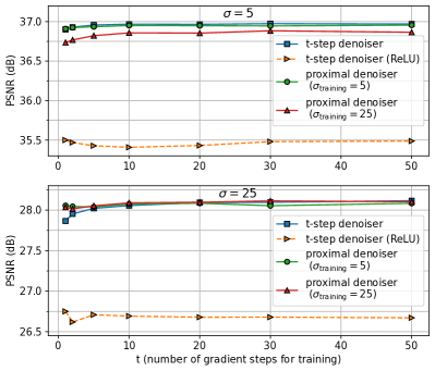
Figure 2: Test denoising performance of CRR-NNs for noise level $\sigma=5/255$ and $\sigma=25/255$ versus the number of gradient steps used for training, the denoiser type ($t$-step vs proximal), and the noise level used for training.

VI-C Biomedical Image Reconstruction

The six CRR-NNs trained on denoising with $t\in\{1,10,50\}$ and $\sigma\in\{5/255,25/255\}$ are now used to solve the following two ill-posed inverse problems.

MRI

The ground-truth images for our MRI experiments are proton-density weighted knee MR images from the fastMRI dataset [70] with fat suppression (PDFS) and without fat suppresion (PD). They are generated from the fully-sampled k-space data. For each of the two categories (PDFS and PD), we create validation and test sets consisting of 10 and 50 images, respectively, where every image is normalized to have a maximum value of one. To gauge the performance of CRR-NNs in various regimes, we experiment with single-coil and multi-coil setups with several acceleration factors. In the single-coil setup, we simulate the measurements by masking the Fourier transform of the ground-truth image. In the multi-coil case, we consider 15 coils, and the measurements are simulated by subsampling the Fourier transforms of the multiplication of the ground-truth images with 15 complex-valued sensitivity maps (these were estimated from the raw k-space data using the ESPIRiT algorithm [71] available in the BART toolbox [72]). For both cases, the subsampling in the Fourier domain is performed with a Cartesian mask that is specified by two parameters: the acceleration $M_{\text{acc}}\in\{2,4,8\}$ and the center fraction $M_{\text{cf}}=0.32/M_{\text{acc}}$. A fraction of $M_{\text{cf}}$ columns in the center of the k-space (low frequencies) is kept, while columns in the other region of the k-space are uniformly sampled so that the expected proportion of selected columns is $1/M_{\text{acc}}$. In addition, Gaussian noise with standard deviation $\sigma_{\mathbf{n}}=$2\text{\cdot}{10}^{-3}$$ is added to the real and imaginary parts of the measurements. The PSNR and SSIM values for each method are computed on the $(320\times 320)$ centered ROI.

Table III: Single-coil MRI.

	2-fold				4-fold
	PSNR		SSIM		PSNR		SSIM
	PD	PDFS	PD	PDFS	PD	PDFS	PD	PDFS
Zero-fill	33.32	34.49	0.871	0.872	27.40	29.68	0.729	0.745
TV	39.22	37.73	0.947	0.917	32.44	32.67	0.833	0.781
PnP-$\beta$CNN	38.77	37.89	0.943	0.924	31.37	31.82	0.832	0.797
CRR-NN	40.95	38.91	0.961	0.934	33.99	33.75	0.880	0.831
PnP-DnCNN [19]	40.52	39.02	0.956	0.935	35.24	34.63	0.884	0.840

Table IV: CRR-NN: Single-coil MRI versus training setup.

			2-fold				4-fold
			PSNR		SSIM		PSNR		SSIM
image	$\sigma_{\mathrm{train}}$	t	PD	PDFS	PD	PDFS	PD	PDFS	PD	PDFS
BSD	5/255	1	40.55	38.71	0.959	0.932	33.32	33.37	0.866	0.819
BSD	5/255	10	40.52	38.69	0.959	0.932	33.30	33.36	0.865	0.817
BSD	5/255	50	40.50	38.67	0.958	0.931	33.29	33.32	0.865	0.816
BSD	25/255	1	40.75	38.84	0.960	0.934	33.62	33.60	0.875	0.828
BSD	25/255	10	40.78	38.81	0.960	0.933	33.63	33.59	0.875	0.826
BSD	25/255	50	40.71	38.77	0.960	0.932	33.57	33.54	0.872	0.824
MRI	5/255	10	40.95	38.91	0.961	0.934	33.99	33.75	0.880	0.831
MRI	25/255	10	40.61	38.73	0.959	0.932	33.93	33.71	0.878	0.830

Table V: Multi-coil MRI.

	4-fold				8-fold
	PSNR		SSIM		PSNR		SSIM
	PD	PDFS	PD	PDFS	PD	PDFS	PD	PDFS
$\mathbf{H}^{T}\mathbf{y}$	27.71	29.94	0.751	0.759	23.80	27.19	0.648	0.681
TV	38.06	37.31	0.935	0.914	32.77	33.38	0.850	0.824
PnP-$\beta$CNN	37.88	37.48	0.934	0.919	32.52	33.30	0.849	0.832
CRR-NN	39.54	38.29	0.950	0.927	34.29	34.50	0.881	0.852
PnP-DnCNN [19]	39.55	38.52	0.947	0.929	35.11	35.14	0.881	0.858

Table VI: CRR-NN: Multi-coil MRI versus training setup.

			4-fold				8-fold
			PSNR		SSIM		PSNR		SSIM
image	$\sigma_{\mathrm{train}}$	t	PD	PDFS	PD	PDFS	PD	PDFS	PD	PDFS
BSD	5/255	1	39.15	38.09	0.947	0.925	33.82	34.22	0.873	0.846
BSD	5/255	10	39.14	38.08	0.946	0.925	33.82	34.20	0.873	0.845
BSD	5/255	50	39.14	38.05	0.946	0.924	33.78	34.16	0.872	0.844
BSD	25/255	1	39.34	38.21	0.948	0.926	34.02	34.35	0.876	0.849
BSD	25/255	10	39.33	38.19	0.948	0.926	34.01	34.34	0.876	0.848
BSD	25/255	50	39.29	38.15	0.948	0.926	33.96	34.29	0.876	0.847
MRI	5/255	10	39.54	38.29	0.950	0.927	34.29	34.50	0.881	0.852
MRI	25/255	10	39.33	38.14	0.947	0.925	34.22	34.40	0.878	0.849

CT

To provide a fair comparison with the ACR method, we now target the CT experiment proposed in [38]. The data consist of human abdominal CT scans for 10 patients provided by Mayo Clinic for the low-dose CT Grand Challenge [73]. The validation set consists of 6 images taken uniformly from the first patient of the training set from [38]. We use the same test set as [38], more precisely, 128 slices with size $(512\times 512)$ that correspond to one patient. The projections of the data are simulated using a parallel-beam acquisition geometry with 200 angles and 400 detectors. Lastly, Gaussian noise with standard deviation $\sigma_{\mathbf{n}}\in\{0.5,1,2\}$ is added to the measurements.

Table VII: CT.

	$\sigma_{\mathbf{n}}$=0.5		$\sigma_{\mathbf{n}}$=1		$\sigma_{\mathbf{n}}$=2
	PSNR	SSIM	PSNR	SSIM	PSNR	SSIM
FBP	32.14	0.697	27.05	0.432	21.29	0.204
TV	36.38	0.936	34.11	0.906	31.57	0.863
PnP-$\beta$CNN	37.19	0.920	34.11	0.873	30.93	0.804
ACR [38, 39]	38.06	0.943	35.12	0.911	32.17	0.868
CRR-NN	39.30	0.947	36.29	0.916	33.16	0.878
PnP-DnCNN [19]	38.93	0.941	36.49	0.921	33.52	0.897

Table VIII: CRR-NN: CT versus training setup.

			$\sigma_{\mathbf{n}}$=0.5		$\sigma_{\mathbf{n}}$=1		$\sigma_{\mathbf{n}}$=2
image	$\sigma_{\mathrm{train}}$	t	PSNR	SSIM	PSNR	SSIM	PSNR	SSIM
BSD	5/255	1	38.84	0.943	35.70	0.907	32.48	0.860
BSD	5/255	10	38.90	0.943	35.73	0.908	32.49	0.860
BSD	5/255	50	38.82	0.940	35.64	0.904	32.47	0.855
BSD	25/255	1	39.01	0.945	35.91	0.913	32.72	0.867
BSD	25/255	10	39.07	0.945	35.95	0.911	32.71	0.867
BSD	25/255	50	39.04	0.944	35.89	0.912	32.71	0.860
CT	5/255	10	39.30	0.947	36.29	0.916	33.15	0.873
CT	25/255	10	38.89	0.945	36.11	0.917	33.16	0.878

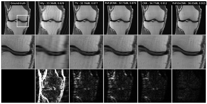
Figure 3: Reconstructed images for the 4-fold accelerated multi-coil MRI experiment. The reported metrics are PSNR and SSIM. The last row shows the squared differences between the reconstructions and the ground-truth image.

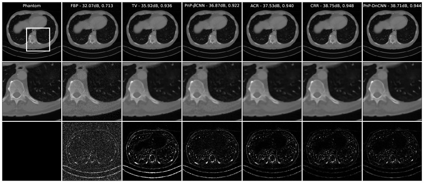
Figure 4: Reconstructed images for the CT experiment with $\sigma_{\mathbf{n}}=0.5$. The reported metrics are PSNR and SSIM. The last row shows the squared differences between the reconstructions and the ground-truth image.

Reconstruction Frameworks

A reconstruction with isotropic TV regularization is computed with FISTA [58], in which $\operatorname{prox}_{R}$ is computed as in [74] to enforce positivity. We also consider reconstructions obtained with the PnP method with (i) provably averaged denoisers $\beta\mathrm{CNN}_{\sigma}$ ($\sigma=5,25$); and (ii) the popular pertained DnCNNs [19] ($\sigma=5,15,40$). The latter are residual denoisers with 1-Lipschitz convolutional layers and batch normalization modules, which yield a non-averaged denoiser with no convergence guarantees for ill-posed problems. To adapt the strength of the denoisers, in addition to the training noise level, we use relaxed denoisers ${\boldsymbol{D}}_{\gamma}=\gamma{\boldsymbol{D}}+(1-\gamma)\mathbf{Id}$ for all denoisers ${\boldsymbol{D}}$, where $\gamma\in(0,1]$ is tuned along with the stepsize $\alpha$ given in (44). We only report the performance of the best-performing setting. The ACR framework [38, 39] yields a convex regularizer for (2) that is specifically designed to the described CT problem. To be consistent with [38, 39], we apply 400 iterations of gradient descent, even though the objective is nonsmooth, and tune the stepsize and $\lambda$. The results are consistent with those reported in [38, 39].

To assess the dependence of CRR-NNs on the image domain, we also train models for Gaussian denoising of CT and MRI images ($t=10$, $\sigma\in\{5/255,25/255\}$). The training procedure is the same as for BSD image denoising, but a larger kernel size of 11 was required to saturate the performance. The learnt filters and activations are included in the Supplementary Material.

The hyperparameters for all these methods are tuned to maximize the average PSNR over the validation set with the coarse-to-fine method given in Appendix -A.

Results and Discussion

For each modality, a reconstruction example is given for each framework in Figures 3 and 4, and additional illustrations are given in the Supplementary Material. The PSNR and SSIM values for the test set given in Tables III, V, and VII attest that CRR-NNs consistently outperform the other frameworks with comparable guarantees. It can be seen from Tables IV, VI, and VIII that the improvements hold for all setups explored to trained CRR-NNs. The training of CRR-NNs on the target image domain allows for an additional small performance boost. The performances of CRR-NNs are close to the ones of PnP-DnCNN, which has however no guarantees and little interpretability. PnP-DnCNN typically yields artifact-free reconstructions but is more prone to over-smoothing (Figure 3) or even to exaggeration of some details in rare cases (see Figures in the Supplementary Material). Lastly, observe that the properly constrained PnP-$\beta$CNN is not always competitive with TV. This confirms the difficulty of training provably 1-Lipchitz CNN, which is also reported for MRI image reconstruction in [66]. Convergence curves for CRR-NNs can be found in the Supplementary Material.

VI-D Under the Hood of the Learnt Regularizers

The filters and activation functions for learnt CRR-NNs with $\sigma\in\{5/255,25/255\}$ and $t=5$ are shown in Figures 5 and 6.

VI-D1 Filters

The impulse responses of the filters vary in orientation and frequency response. This indicates that the CRR-NN decouples the frequency components of patches. The learnt kernels typically come in groups that are reminiscent of 2D steerable filters [75, 76]. Interestingly, their support is wider when the denoising task is carried out for $\sigma=25/255$ than for $\sigma=5/255$.

VI-D2 Activation Functions

The linear splines converge to simple functions throughout the training. The regularization (36) leads to even simpler ones without a compromise in performance. Most of them end up with 3 linear regions, with their shape being reminiscent of the clipping function $\mathrm{Clip}(x)=\mathrm{sign}(x)\min(|x|,1)$. The learnt regularizer is closely related to $\ell_{1}$-norm based regularization as many of the learnt convex profiles $\psi_{i}$ resemble some smoothed version of the absolute-value function.

VI-D3 Pruning CRR-NNs

Since the NN has a simple architecture, it can be efficiently pruned before inference by removal of the filters associated with almost-vanishing activation functions. This yields models with typically between $3000$ and $5000$ parameters and offers a clear advantage over deep models, which can usually not be pruned efficiently.

VI-D4 A Signal-Processing Interpretation

Given that the gradient-step operator $\mathbf{x}\mapsto(\mathbf{x}-\alpha\mathbf{W}^{T}\boldsymbol{\sigma}(\mathbf{W}\mathbf{x}))$ of the learnt regularizer is expected to remove some noise from $\mathbf{x}$, the 1-hidden-layer CNN $\mathbf{W}^{T}\boldsymbol{\sigma}(\mathbf{W}\mathbf{\cdot})$ is expected to extract noise. The response of $\mathbf{x}$ to the learnt filters forms the high-dimensional representation $\mathbf{W}\mathbf{x}$ of $\mathbf{x}$. The clipping function preserves the small responses to the filters, while it cuts the large ones. Hence, the estimated noise $\mathbf{W}^{T}\boldsymbol{\sigma}(\mathbf{W}\mathbf{x})$ is reconstructed by essentially removing the components of $\mathbf{x}$ that exhibit a significant correlation with the kernels of the filters. All in all, the learning of the activation functions leads closely to wavelet- or framelet-like denoising. Indeed, the proximal operator of $\mathbf{x}\mapsto\|\mathrm{DWT}(\mathbf{x})\|_{1}$ is given by

$$\mathrm{prox}_{\|\mathrm{DWT}(\mathbf{\cdot})\|_{1}}(\mathbf{x}) =\mathrm{IDWT}(\mathrm{soft}(\mathrm{DWT}(\mathbf{x})))$$

$$=\mathbf{x}-\mathrm{IDWT}(\mathrm{clip}(\mathrm{DWT}(\mathbf{x}))),$$ (48)

where $\mathrm{soft}(\cdot)$ is the soft-thresholding function, $\mathrm{DWT}$ and $\mathrm{IDWT}$ are the orthogonal discrete wavelet transform and its inverse, respectively. The equivalent formulation with the clipping function follows from $\mathrm{IDWT}(\mathrm{DWT}(\mathbf{x}))=\mathbf{x}$ and $\mathrm{soft}(\mathbf{x})=(\mathbf{x}-\mathrm{clip}(\mathbf{x}))$. The soft-thresholding function is used for direct denoising while the clipping function is tailored to residual denoising. Note that the given analogy is, however, limited since the learnt filters are not orthonormal ($\mathbf{W}^{T}\mathbf{W}\neq\mathbf{I}$).

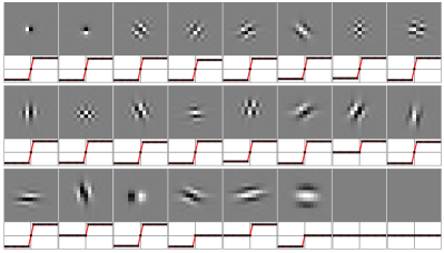
Figure 5: Impulse response of the filters and activation functions of the CRR-NN trained with $\sigma=5$. The crosses indicate the knots of the splines. For the 8 missing filters, the associated activation functions were numerically identically zero.

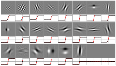
Figure 6: Impulse response of the filters and activation functions of the CRR-NN trained with $\sigma=25/255$.

VI-D5 Role of the Scaling Factor

To clarify the role of the scaling factor $\mu$ introduced in (42), we investigate a toy problem on the space of one-dimensional signals. Since these can be interpreted as images varying along a single direction, a signal regularizer $R_{1}$ can be obtained from $R_{\boldsymbol{\theta}}$ by replacing the 2D convolutional filters with 1D convolutional filters whose kernels are the ones of $R_{\boldsymbol{\theta}}$ summed along a direction. Next, we seek a compactly supported signal with fixed mass that has minimum regularization cost, as in

$$\hat{\mathbf{c}}=\operatorname*{arg\,min}\limits_{\mathbf{c}\in\operatorname{{\mathbb{R}}}^{d}}R_{1}(\mu\mathbf{c})\,\,\,\text{s.t.}\,\,\,\begin{cases}\mathbf{1}^{T}\mathbf{c}=1,\\ \mathbf{c}_{k}=0,&\forall k\not\in[k_{1},k_{2}].\end{cases}$$ (49)

The solutions for various values of $\mu$ are shown in Figure 7. Small values of $\mu$ promote smooth functions in a way reminiscent of the Tikhonov regularizer applied to finite differences. Large values of $\mu$ promote functions with constant portions and, conjointly, allows for sharp jumps, which is reminiscent of the TV regularizer. This reasoning is in agreement with the shape of the activation functions shown in Figures 5 and 6. Indeed, an increase in $\mu$ allows one to enlarge the region where the regularizer has constant gradients, while a decrease of $\mu$ allows one to enlarge the region where the regularizer has linear gradients.

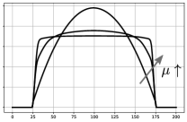
Figure 7: Solutions of the one-dimensional problem (49) for increasing values of $\mu$. The plotted functions are supported in $[25,175]$ and minimize the learnt regularizer given a unit sum of their values.

VII Conclusion

We have proposed a framework to learn universal convex-ridge regularizers with adaptive profiles. When applied to inverse problems, it is competitive with those recent deep-learning approaches that also prioritize the reliability of the method. Not only CRR-NNs are faster to train, but they also offer improvements in image quality. The findings raise the question of whether shallow models such as CRR-NNs, despite their small number of parameters, already offer optimal performance among methods that rely either on a learnable convex regularizer or on the PnP framework with a provably averaged denoiser. In the future, CRR-NNs could be fine-tuned on specific modalities via the use of $\mathbf{H}$ for training. This could further improve the reconstruction quality, as observed when shifting from PnP to deep unrolled algorithms while maintaining the guarantees.

-A Hyperparameter Tuning

The parameters $\lambda$ and $\mu$ used in (42) can be tuned with a coarse-to-fine approach. Given the performance on the $3\times 3$ grid $\{(\gamma_{\lambda})^{-1}\lambda,\lambda,\gamma_{\lambda}\lambda\}\times\{(\gamma_{\mu})^{-1}\mu,\mu,\gamma_{\mu}\mu\}$, we identify the best values $\lambda^{*}$ and $\mu^{*}$ on this subset and move on to the next iteration as follows:

• if $\lambda^{*}=\lambda$, we refine the search grid by reducing $\gamma_{\mu}$ to $(\gamma_{\mu})^{\zeta}$, $\zeta<1$;

• otherwise, $\lambda$ is updated to $\lambda^{*}$.

A similar update is performed for the scaling parameter. The search is terminated when both $\gamma_{\lambda}$ and $\gamma_{\mu}$ are smaller than a threshold, typically, $1.01$. In practice, we initialized $\gamma_{\lambda}=\gamma_{\mu}=4$ and set $\zeta=0.5$. The method usually requires between $50$ and $100$ evaluations on tuples $(\lambda,\mu)$ on the validation set before it terminates. The proposed approach is predicated on the observation that the optimization landscape in the $(\lambda,\mu)$ domain is typically well-behaved. The same principles apply to tune a single hyperparameter, as found in the TV and the PnP-$\beta$CNN methods. Let us remark that the performances were found to change only slowly with the scaling parameter $\mu$ for the MRI and CT experiments. Hence, in practice, it is enough to tune $\mu$ very coarsely.

Supplementary Material

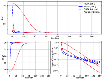
Figure 8: Example of convergence curves (denoising).

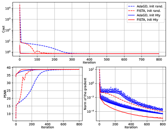
Figure 9: Example of convergence curves (MRI).

Convergence Curves

In this section, we present convergence curves for image denoising (Figure 8), MRI reconstruction (Figure 9), and CT reconstruction (Figure 10) with CRR-NNs. The underlying objective is minimized with FISTA[58] and AdaGD5[56], which both converge generally fast. Depending on the task and the desired accuracy, one or the other might be faster. The observed gradient-norm oscillations for AdaGD are typical for this method and unrelated to CRR-NNs [56]. Finally, note that the initialization affects the convergence speed, but does not impact the reconstruction quality. This differs significantly from PnP methods that deploy loosely constrained denoisers.

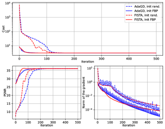
Figure 10: Example of convergence curves (CT).

Activations and Filters

We provide the filters and activations of a CRR-NN trained for the denoising of CT images (Figure 14) and of MRI images (Figure 14). Compared to the training on the BSD500 dataset, larger kernel sizes were needed to saturate the performances.

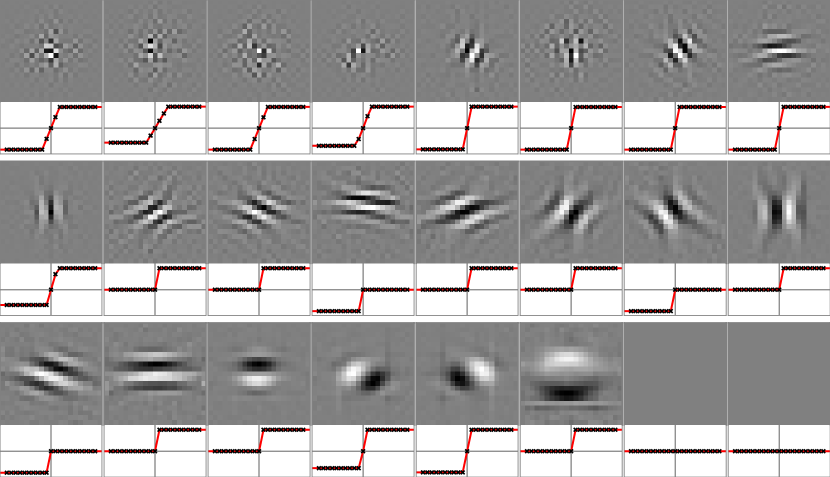
Figure 11: Impulse response of the filters and activation functions of the CRR-NN trained to denoise CT images.

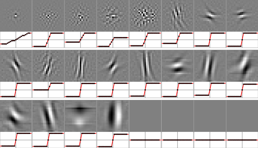
Figure 12: Impulse response of the filters and activation functions of the CRR-NN trained to denoise MRI images.

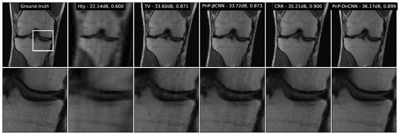
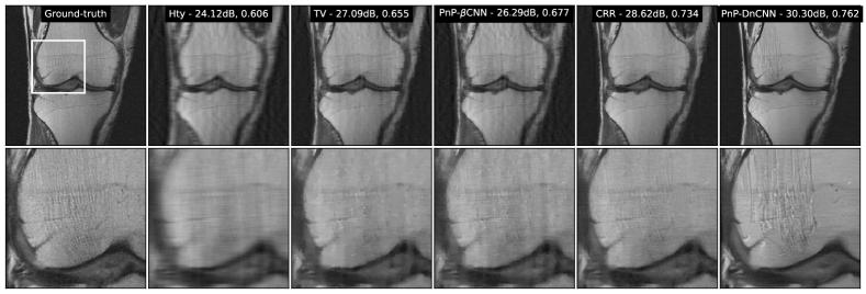
Figure 13: Reconstructions for the 8-fold accelerated multi-coil MRI experiment.

Figure 14: Reconstructions for the 4-fold accelerated single-coil MRI experiment. Note the unexpected behavior of DnCNN.

Reconstructed images

MRI

In Figures 14 and 14, we present reconstructions from multi- and single-coil MRI measurements, and report their PSNR and SSIM as metrics. The reconstruction task in Figure 14 is particularly challenging. In this regime, it can be observed that the loosely constrained PnP-DnCNN exaggerates some structures, even though the metrics remain acceptable.

CT

In Figures 16 and 16, we provide reconstructions for the CT experiments with noise levels $\sigma_{\mathbf{n}}=1,2$ in the measurements. The reported metrics are PSNR and SSIM.

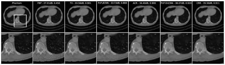
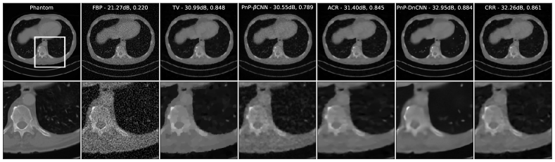
Figure 15: Reconstructed images for the CT experiment with $\sigma_{\mathbf{n}}=1.0$.

Figure 16: Reconstructed images for the CT experiment with $\sigma_{\mathbf{n}}=2.0$.

References

- [1] A. Ribes and F. Schmitt, “Linear inverse problems in imaging,” IEEE Signal Processing Magazine, vol. 25, no. 4, pp. 84–99, 2008.
- [2] M. T. McCann and M. Unser, “Biomedical image reconstruction: From the foundations to deep neural networks,” Foundations and Trends® in Signal Processing, vol. 13, no. 3, pp. 283–359, 2019.
- [3] A. N. Tikhonov, “Solution of incorrectly formulated problems and the regularization method,” Soviet Mathematics, vol. 4, pp. 1035–1038, 1963.
- [4] L. I. Rudin, S. Osher, and E. Fatemi, “Nonlinear total variation based noise removal algorithms,” Physica D: Nonlinear Phenomena, vol. 60, no. 1-4, pp. 259–268, 1992.
- [5] D. L. Donoho, “Compressed sensing,” IEEE Transactions on Information Theory, vol. 52, no. 4, pp. 1289–1306, 2006.
- [6] E. J. Candès and M. B. Wakin, “An introduction to compressive sampling,” IEEE Signal Processing Magazine, vol. 25, no. 2, pp. 21–30, 2008.
- [7] S. Arridge, P. Maass, O. Öktem, and C.-B. Schönlieb, “Solving inverse problems using data-driven models,” Acta Numerica, vol. 28, pp. 1–174, 2019.
- [8] G. Ongi, A. Jalal, C. A. Metzle, R. G. Baraniuk, A. G. Dimakis, and R. Willett, “Deep learning techniques for inverse problems in imaging,” IEEE Journal on Selected Areas in Information Theory, vol. 1, no. 1, pp. 39–56, 2020.
- [9] V. Antun, F. Renna, C. Poon, B. Adcock, and A. C. Hansen, “On instabilities of deep learning in image reconstruction and the potential costs of AI,” Proceedings of the National Academy of Sciences, vol. 117, no. 48, pp. 30 088–30 095, 2020.
- [10] N. M. Gottschling, V. Antun, B. Adcock, and A. C. Hansen, “The troublesome kernel: why deep learning for inverse problems is typically unstable,” arXiv:2001.01258, 2020.
- [11] K. H. Jin, M. T. McCann, E. Froustey, and M. Unser, “Deep convolutional neural network for inverse problems in imaging,” IEEE Transactions on Image Processing, vol. 26, no. 9, pp. 4509–4522, 2017.
- [12] H. Chen, Y. Zhang, W. Zhang, P. Liao, K. Li, J. Zhou, and G. Wang, “Low-dose CT via convolutional neural network,” Biomedical Optics Express, vol. 8, no. 2, pp. 679–694, 2017.
- [13] B. Zhu, J. Z. Liu, S. F. Cauley, B. R. Rosen, and M. S. Rosen, “Image reconstruction by domain-transform manifold learning,” Nature, vol. 555, no. 7697, pp. 487–492, 2018.
- [14] C. M. Hyun, H. P. Kim, S. M. Lee, S. Lee, and J. K. Seo, “Deep learning for undersampled MRI reconstruction,” Physics in Medicine & Biology, vol. 63, no. 13, p. 135007, 2018.
- [15] P. Hagemann and S. Neumayer, “Stabilizing invertible neural networks using mixture models,” Inverse Problems, vol. 37, no. 8, p. 085002, 2021.
- [16] S. V. Venkatakrishnan, C. A. Bouman, and B. Wohlberg, “Plug-and-Play priors for model based reconstruction,” in IEEE Global Conference on Signal and Information Processing, 2013, pp. 945–948.
- [17] S. H. Chan, X. Wang, and O. A. Elgendy, “Plug-and-Play ADMM for image restoration: Fixed-point convergence and applications,” IEEE Transactions on Computational Imaging, vol. 3, no. 1, pp. 84–98, 2016.
- [18] Y. Romano, M. Elad, and P. Milanfar, “The little engine that could: Regularization by denoising (RED),” SIAM Journal on Imaging Sciences, vol. 10, no. 4, pp. 1804–1844, 2017.
- [19] E. Ryu, J. Liu, S. Wang, X. Chen, Z. Wang, and W. Yin, “Plug-and-Play methods provably converge with properly trained denoisers,” in Proceedings of the 36th International Conference on Machine Learning, ser. Proceedings of Machine Learning Research, vol. 97. PMLR, 09–15 June 2019, pp. 5546–5557.
- [20] P. Bohra, D. Perdios, A. Goujon, S. Emery, and M. Unser, “Learning Lipschitz-controlled activation functions in neural networks for Plug-and-Play image reconstruction methods,” in NeurIPS 2021 Workshop on Deep Learning and Inverse Problems, 2021.
- [21] M. Hasannasab, J. Hertrich, S. Neumayer, G. Plonka, S. Setzer, and G. Steidl, “Parseval proximal neural networks,” The Journal of Fourier Analysis, vol. 26, p. 59, 2020.
- [22] J. Hertrich, S. Neumayer, and G. Steidl, “Convolutional proximal neural networks and Plug-and-Play algorithms,” Linear Algebra and its Applications, vol. 631, pp. 203–234, 2021.
- [23] H. Gupta, K. H. Jin, H. Q. Nguyen, M. T. McCann, and M. Unser, “CNN-based projected gradient descent for consistent CT image reconstruction,” IEEE Transactions on Medical Imaging, vol. 37, no. 6, pp. 1440–1453, 2018.
- [24] S. Hurault, A. Leclaire, and N. Papadakis, “Gradient step denoiser for convergent Plug-and-Play,” in International Conference on Learning Representations, 2022.
- [25] S. Roth and M. J. Black, “Fields of experts,” International Journal of Computer Vision, vol. 82, no. 2, pp. 205–229, 2009.
- [26] Y. Chen, R. Ranftl, and T. Pock, “Insights into analysis operator learning: From patch-based sparse models to higher order MRFs,” IEEE Transactions on Image Processing, vol. 23, pp. 1060–72, 2014.
- [27] A. Effland, E. Kobler, K. Kunisch, and T. Pock, “Variational networks: An optimal control approach to early stopping variational methods for image restoration,” Journal of Mathematical Imaging and Vision, vol. 62, no. 3, pp. 396–416, 2020.
- [28] S. Lunz, O. Öktem, and C.-B. Schönlieb, “Adversarial regularizers in inverse problems,” Advances in Neural Information Processing Systems, vol. 31, 2018.
- [29] M. Duff, N. D. F. Campbell, and M. J. Ehrhardt, “Regularising inverse problems with generative machine learning models,” arXiv:2107.11191, 2021.
- [30] H. Li, J. Schwab, S. Antholzer, and M. Haltmeier, “NETT: Solving inverse problems with deep neural networks,” Inverse Problems, vol. 36, no. 6, p. 065005, 2020.
- [31] E. Kobler, A. Effland, K. Kunisch, and T. Pock, “Total deep variation for linear inverse problems,” in IEEE/CVF Conference on Computer Vision and Pattern Recognition (CVPR), June 2020.
- [32] R. Cohen, Y. Blau, D. Freedman, and E. Rivlin, “It has potential: Gradient-driven denoisers for convergent solutions to inverse problems,” Advances in Neural Information Processing Systems, vol. 34, 2021.
- [33] S. Hurault, A. Leclaire, and N. Papadakis, “Proximal denoiser for convergent Plug-and-Play optimization with nonconvex regularization,” in Proceedings of the 39th International Conference on Machine Learning, ser. Proceedings of Machine Learning Research, vol. 162. PMLR, 17–23 July 2022, pp. 9483–9505.
- [34] R. Fermanian, M. Le Pendu, and C. Guillemot, “Pnp-reg: Learned regularizing gradient for plug-and-play gradient descent,” SIAM Journal on Imaging Sciences, vol. 16, no. 2, pp. 585–613, 2023. [Online]. Available: https://doi.org/10.1137/22M1490843
- [35] E. Kobler, T. Klatzer, K. Hammernik, and T. Pock, “Variational networks: Connecting variational methods and deep learning,” in Pattern Recognition, 2017, pp. 281–293.
- [36] P. Nair and K. N. Chaudhury, “On the construction of averaged deep denoisers for image regularization,” arXiv:2207.07321, 2022.
- [37] J.-C. Pesquet, A. Repetti, M. Terris, and Y. Wiaux, “Learning maximally monotone operators for image recovery,” SIAM Journal on Imaging Sciences, vol. 14, no. 3, pp. 1206–1237, 2021.
- [38] S. Mukherjee, S. Dittmer, Z. Shumaylov, S. Lunz, O. Öktem, and C.-B. Schönlieb, “Learned convex regularizers for inverse problems,” arXiv:2008.02839, 2021.
- [39] S. Mukherjee, C.-B. Schönlieb, and M. Burger, “Learning convex regularizers satisfying the variational source condition for inverse problems,” in NeurIPS Workshop on Deep Learning and Inverse Problems, 2021.
- [40] B. Amos, L. Xu, and J. Z. Kolter, “Input convex neural networks,” in Proceedings of the 34th International Conference on Machine Learning, ser. Proceedings of Machine Learning Research, vol. 70. PMLR, 06–11 August 2017, pp. 146–155.
- [41] H. Q. Nguyen, E. Bostan, and M. Unser, “Learning convex regularizers for optimal Bayesian denoising,” IEEE Transactions on Signal Processing, vol. 66, no. 4, pp. 1093–1105, 2017.
- [42] G. Peyré and J. M. Fadili, “Learning analysis sparsity priors,” in SampTA’11, 2011, p. 4.
- [43] Y. Chen, T. Pock, and H. Bischof, “Learning -based analysis and synthesis sparsity priors using bi-level optimization,” in 26th Neural Information Processing Systems Confercence, 2012.
- [44] L. B. Willner, “On the distance between polytopes,” Quarterly of Applied Mathematics, vol. 26, no. 2, pp. 207–212, 1968.
- [45] S. Bai, J. Z. Kolter, and V. Koltun, “Deep equilibrium models,” in Advances in Neural Information Processing Systems, vol. 32, 2019.
- [46] D. Gilton, G. Ongie, and R. Willett, “Deep equilibrium architectures for inverse problems in imaging,” IEEE Transactions on Computational Imaging, vol. 7, pp. 1123–1133, 2021.
- [47] A. Pramanik, M. B. Zimmerman, and M. Jacob, “Memory-efficient model-based deep learning with convergence and robustness guarantees,” IEEE Transactions on Computational Imaging, vol. 9, pp. 260–275, 2023.
- [48] A. Pramanik, H. K. Aggarwal, and M. Jacob, “Deep generalization of structured low-rank algorithms (deep-slr),” IEEE Transactions on Medical Imaging, vol. 39, no. 12, pp. 4186–4197, 2020.
- [49] H. K. Aggarwal, M. P. Mani, and M. Jacob, “Modl: Model-based deep learning architecture for inverse problems,” IEEE Transactions on Medical Imaging, vol. 38, no. 2, pp. 394–405, 2019.
- [50] P. Bohra, J. Campos, H. Gupta, S. Aziznejad, and M. Unser, “Learning activation functions in deep (spline) neural networks,” IEEE Open Journal of Signal Processing, vol. 1, pp. 295–309, 2020.
- [51] M. Unser, “A representer theorem for deep neural networks,” Journal of Machine Learning Research, vol. 20, no. 110, pp. 1–30, 2019.
- [52] T. Miyato, T. Kataoka, M. Koyama, and Y. Yoshida, “Spectral normalization for generative adversarial networks,” in International Conference on Learning Representations, 2018.
- [53] S. W. Fung, H. Heaton, Q. Li, D. McKenzie, S. Osher, and W. Yin, “JFB: Jacobian-free backpropagation for implicit networks,” in Proceedings of the AAAI Conference on Artificial Intelligence, 2022.
- [54] M. Unser, “Splines: A perfect fit for signal and image processing,” IEEE Signal Processing Magazine, vol. 16, no. 6, pp. 22–38, November 1999, IEEE-SPS best paper award.
- [55] X. Xu, J. Liu, Y. Sun, B. Wohlberg, and U. S. Kamilov, “Boosting the performance of Plug-and-Play priors via denoiser scaling,” in 54th Asilomar Conference on Signals, Systems, and Computers, 2020, pp. 1305–1312.
- [56] Y. Malitsky and K. Mishchenko, “Adaptive gradient descent without descent,” in Proceedings of the 37th International Conference on Machine Learning, ser. Proceedings of Machine Learning Research, H. D. III and A. Singh, Eds., vol. 119. PMLR, 13–18 Jul 2020, pp. 6702–6712. [Online]. Available: https://proceedings.mlr.press/v119/malitsky20a.html
- [57] P. Latafat, A. Themelis, L. Stella, and P. Patrinos, “Adaptive proximal algorithms for convex optimization under local lipschitz continuity of the gradient,” 2023.
- [58] A. Beck and M. Teboulle, “A fast iterative shrinkage-thresholding algorithm for linear inverse problems,” SIAM journal on imaging sciences, vol. 2, no. 1, pp. 183–202, 2009.
- [59] P. L. Combettes and V. R. Wajs, “Signal recovery by proximal forward-backward splitting,” Multiscale Modeling & Simulation, vol. 4, no. 4, pp. 1168–1200, 2005.
- [60] S. Ducotterd, A. Goujon, P. Bohra, D. Perdios, S. Neumayer, and M. Unser, “Improving lipschitz-constrained neural networks by learning activation functions,” 2022.
- [61] J. Liu, S. Asif, B. Wohlberg, and U. Kamilov, “Recovery analysis for Plug-and-Play priors using the restricted eigenvalue condition,” in Advances in Neural Information Processing Systems, 2021.
- [62] A. Pramanik and M. Jacob, “Improved model based deep learning using monotone operator learning (MOL),” in 2022 IEEE 19th International Symposium on Biomedical Imaging (ISBI), 2022, pp. 1–4.
- [63] T. Huster, C.-Y. J. Chiang, and R. Chadha, “Limitations of the Lipschitz constant as a defense against adversarial examples,” in Joint European Conference on Machine Learning and Knowledge Discovery in Databases, 2018, pp. 16–29.
- [64] C. Anil, J. Lucas, and R. Grosse, “Sorting out Lipschitz function approximation,” in Proceedings of the 36th International Conference on Machine Learning, ser. Proceedings of Machine Learning Research, vol. 97. PMLR, 2019, pp. 291–301.
- [65] S. Neumayer, A. Goujon, P. Bohra, and M. Unser, “Approximation of Lipschitz functions using deep spline neural networks,” SIAM Journal on Mathematics of Data Science, vol. 5, no. 2, pp. 306–322, 2023.
- [66] J. R. Chand and M. Jacob, “Multi-scale energy (muse) plug and play framework for inverse problems,” 2023.
- [67] K. Zhang, W. Zuo, Y. Chen, D. Meng, and L. Zhang, “Beyond a Gaussian denoiser: Residual learning of deep CNN for image denoising,” IEEE Transactions on Image Processing, vol. 26, no. 7, pp. 3142–3155, 2017.
- [68] P. Arbeláez, M. Maire, C. Fowlkes, and J. Malik, “Contour detection and hierarchical image segmentation,” IEEE Transactions on Pattern Analysis and Machine Intelligence, vol. 33, no. 5, pp. 898–916, 2011.
- [69] A. Chambolle, “An algorithm for total variation minimization and applications,” Journal of Mathematical imaging and vision, vol. 20, no. 1, pp. 89–97, 2004.
- [70] F. Knoll, J. Zbontar, A. Sriram, M. J. Muckley, M. Bruno, A. Defazio, M. Parente, K. J. Geras, J. Katsnelson, H. Chandarana, Z. Zhang, M. Drozdzalv, A. Romero, M. Rabbat, P. Vincent, J. Pinkerton, D. Wang, N. Yakubova, E. Owens, C. L. Zitnick, M. P. Recht, D. K. Sodickson, and Y. W. Lui, “fastMRI: A publicly available raw k-space and DICOM dataset of knee images for accelerated MR image reconstruction using machine learning,” Radiology: Artificial Intelligence, vol. 2, no. 1, 2020.
- [71] M. Uecker, P. Lai, M. J. Murphy, P. Virtue, M. Elad, J. M. Pauly, S. S. Vasanawala, and M. Lustig, “ESPIRiT-an eigenvalue approach to autocalibrating parallel MRI: Where SENSE meets GRAPPA,” Magn. Reson. Med., vol. 71, no. 3, pp. 990–1001, Mar. 2014.
- [72] M. Uecker, P. Virtue, F. Ong, M. J. Murphy, M. T. Alley, S. S. Vasanawala, and M. Lustig, “Software toolbox and programming library for compressed sensing and parallel imaging,” in ISMRM Workshop on Data Sampling and Image Reconstruction, 2013, p. 41.
- [73] C. McCollough, “TU-FG-207A-04: Overview of the low dose CT Grand Challenge,” Medical Physics, vol. 43, no. 6Part35, pp. 3759–3760, 2016.
- [74] A. Beck and M. Teboulle, “Fast gradient-based algorithms for constrained total variation image denoising and deblurring problems,” IEEE Transactions on Image Processing, vol. 18, no. 11, pp. 2419–2434, 2009.
- [75] W. T. Freeman and E. H. Adelson, “The design and use of steerable filters,” IEEE Transactions on Pattern Analysis and Machine Intelligence, vol. 13, no. 9, pp. 891–906, 1991.
- [76] M. Unser and N. Chenouard, “A unifying parametric framework for 2D steerable wavelet transforms,” SIAM Journal on Imaging Sciences, vol. 6, no. 1, pp. 102–135, 2013.
- [77] Y. Nesterov, Smooth Convex Optimization. Boston, MA: Springer US, 2004, pp. 51–110. [Online]. Available: https://doi.org/10.1007/978-1-4419-8853-9_2