Macroeconomic Effects of Active Labour Market Policies:
A Novel Instrumental Variables Approach

This study evaluates the macroeconomic effects of active labour market policies (ALMP) in Germany over the period 2005 to 2018. We propose a novel identification strategy to overcome the simultaneity of ALMP and labour market outcomes at the regional level. It exploits the imperfect overlap of local labour markets and local employment agencies that decide on the local implementation of policies. Specifically, we instrument for the use of ALMP in a local labour market with the mix of ALMP implemented outside this market but in local employment agencies that partially overlap with this market. We find no effects of short-term activation measures and further vocational training on aggregate labour market outcomes. In contrast, wage subsidies substantially increase the share of workers in unsubsidised employment while lowering long-term unemployment and welfare dependency. Our results suggest that negative externalities of ALMP partially offset the effects for program participants and that some segments of the labour market benefit more than others.
Keywords: active labour market policies; macroeconomic evaluation; instrumental variables

JEL Codes: C26, H43, J64, J68

1 Introduction

Active labour market policies (ALMP) aim at improving employment prospects of jobseekers, at integrating them into the labour market and thereby reducing unemployment. They include a variety of policy instruments such as counselling and employment services, labour market training, and subsidised employment. Many developed countries invested heavily into such programs over the last decades and to this day, public spending on ALMP remains high at 0.2 to 2% of GDP in EU countries (European Commission, 2022). A large literature analyses individual-level effects of these policies, i.e. whether participation in a program increases the employment probability of participants. This literature finds small or negative effects in the short run but positive effects in the long run, with larger gains for programs that are human capital intensive (see e.g. Card et al., 2018).

Comparing individual gains with the associated investments is not sufficient to judge the overall cost-effectiveness of ALMP. These policies may have the intended effects on program participants but can be accompanied by negative spillover effects on non-participants (Abbring and Heckman, 2007). Such spillovers may work through wage-setting and labour-demand incentives. For example, if programs change relative wage costs, firms might create jobs for program participants and replace jobs for other workers, possibly resulting in a net reduction in labour demand (see e.g. Calmfors, 1994). Recently, a number of contributions provide direct empirical evidence for adverse effects of ALMP on non-participants (Crépon et al., 2013; Ferracci et al., 2014; Gautier et al., 2018; Caria et al., 2022). Furthermore, deadweight losses may occur if program participants would have been hired also in absence of the program. Overall, the existing evidence on the aggregate effects of ALMP remains mixed. An important reason are methodological challenges inherent to macroeconomic evaluations, in particular the simultaneous determination of policies and labour market outcomes at the aggregate level.

In this paper, we study macroeconomic effects of different types of ALMP in Germany and propose a novel identification strategy to overcome these challenges. It is based on the idea that local labour markets are not perfectly coinciding with administrative areas where policy decisions are being made. In Germany, 156 local employment agencies decide on the regional implementation of these policies with large discretion. At the same time, the country is characterised by a decentralised economic structure with several local labour markets. Together, these features provide an ideal laboratory for our macroeconomic evaluation study. Specifically, we analyse how regional labour market outcomes such as the unemployment and employment rates were affected by the intensity of three types of policies: short-term activation measures, further vocational training and wage subsidies.

Our analysis proceeds in two steps. First, we construct precisely-delineated local labour markets based on commuting flows between municipalities. Second, we estimate the effect of the policy use on aggregate labour market outcomes in these markets using a dynamic panel data model. To address simultaneity, we instrument the policy use in a labour market with the policy use in municipalities of local employment agencies that partially overlap with this labour market but lie outside its borders. Our estimation is based on rich administrative data at the individual level, which we aggregate to the labour market level and by quarter over the period 2005 to 2018.

Our findings suggest that the effectiveness of ALMP in reducing unemployment or increasing employment in the aggregate is limited. We find no significant effects for short measures and vocational training programs. Wage subsidies, on the other hand, substantially increase the aggregate employment rate. A 10 percentage point increase in the share of unemployed that receive wage subsidies increases the unsubsidised employment rate by 3 percentage points in the long run. This increase is explained by a lower fraction of workers on welfare and in precarious work. Wage subsidies are thus effective in preventing long-term unemployment and the dependence on state benefits. We also find suggestive evidence for some labour market segments benefiting more from the policies. For example, workers older than 50 experience an increase in unsubsidised employment and a corresponding decrease in unemployment as response to higher intensity of training. This age group also experiences the largest effects of wage subsidies on the employment rate.

We make two main contributions to the literature evaluating ALMP. As our first contribution, we propose a new approach to address the methodological problems in macroeconomic evaluations of ALMP. Existing studies have mostly relied on the variation in the policy use between administrative areas such as countries or smaller entities within a country to identify the aggregate effects of such policies. This poses two types of challenges for identification. First, geographical areas delineated by administrative borders are not necessarily the economic entities of interest. If there exist strong economic ties across administrative borders, the effects of policies introduced in one of the areas might spill over to the other. Some contributions have addressed this issue by controlling for spatially correlated spillover effects (e.g. Fertig et al., 2006b; Hujer et al., 2009; Dauth et al., 2016). Second, if policy decisions are made at the same geographical level at which outcomes are measured, this complicates the separate identification of cause and effect. Previous attempts to mitigate the simultaneity problem use transformations of policy variables such as ratios (Calmfors and Skedinger, 1995), lagged policy variables (Puhani, 2003; Fertig et al., 2006b; Wapler et al., 2018, 2022), or lagged measures as instrumental variables (Nickell, 1997, 1998; Nickell and Layard, 1999; Johansson, 2001; Estevaõ, 2003; Dahlberg and Forslund, 2005; Bassanini and Duval, 2007; Hujer et al., 2009; Dauth et al., 2016; Escudero, 2018). Contributions based on truly exogenous variation are rare and often focus on specific programs. Crépon et al. (2013) use a randomised experiment for measuring spillover effects of a job search program for young university dropouts, Gautier et al. (2018) rely on a difference-in-differences approach to estimate the effects of a job search assistance program.

In our empirical approach we circumvent the issue of regional spillover effects by estimating effects at the local labour market level. These markets form self-contained regions and are less likely to have pronounced economic interdependencies. Relying on local labour markets further allows us to exploit a novel source of exogenous variation in policy use at the regional level. Our instruments rely on the imperfect overlap between local labour markets and administrative regions in charge of policy decisions and are less likely to be endogenously determined compared to lagged policy variables.

As our second contribution we provide a comprehensive evaluation of ALMP. Thereby, we expand the knowledge on the macroeconomic effects of ALMP more generally. Existing studies often derive their econometric specification from the standard matching function (Pissarides, 2000) and focus on a single outcome: the outflows of jobseekers into employment. These papers find little or no significant effects of ALMP (Boeri and Burda, 1996; Puhani, 2003; Fertig et al., 2006b; Hujer et al., 2009; Dauth et al., 2016; Wapler et al., 2022). Other papers that consider the effects of ALMP on the unemployment rate and employment rate also remain largely inconclusive about the effectiveness of these policies (Nickell and Layard, 1999; Blanchard and Wolfers, 2000; Dahlberg and Forslund, 2005; Bassanini and Duval, 2007; Altavilla and Caroleo, 2013; Estevaõ, 2003). More recent evidence suggests that the effects of ALMP might depend on the implementation of the policies (Escudero, 2018) and on regional labour market conditions (Altavilla and Caroleo, 2013; Wapler et al., 2022). Furthermore, the microeconomic evidence on ALMP suggests that program effects vary significantly with the characteristics of participants (e.g. Heckman et al., 1997; Bitler et al., 2006; Bergemann and Van den Berg, 2008; Behaghel et al., 2014). These heterogeneities might also materialise at the macroeconomic level. Escudero (2018) for example finds ALMP to be more effective for the population of low-skilled workers. Our reduced-form approach in combination with a unique administrative dataset allows us to shed light on new aspects of the effectiveness of ALMP. We use quarterly variation over a long time period of 14 years and consider a variety of outcomes that have not been studied in the literature so far. Furthermore, this gives us the opportunity to explore possible heterogeneity in the program effectiveness for different segments of the labour market.

The remainder of the paper is structured as follows. Section 2 introduces the institutional setting in Germany and the policies of interest. Section 3 provides a theoretical background on possible effects. Section 4 describes the empirical strategy and the data. Section 5 presents the main results and Section 6 provides a number of robustness checks. Section 7 concludes.

2 Institutional Setting and Policies

We evaluate the macroeconomic effects of ALMP in Germany for the years 2005 to 2018. Prior to this period, German labour market institutions were heavily reformed by the Job-AQTIV legislation and the Hartz reforms. Our analysis focuses on policies that are defined in the German Social Code (SGB) III and are directed at jobseekers receiving unemployment insurance (UI) benefits. The programs are implemented by local employment agencies (shortly referred to as employment agencies or agencies in the following) and financed by mandatory contributions of employers and employees to national unemployment insurance. We only consider so-called discretionary measures, which cover the main instruments of ALMP. In particular, we cover short-term activation measures, training and wage subsidies. These three types of programs are largest in scope and most likely to generate direct and indirect effects at the aggregate level (Abbring and Heckman, 2007; Imbens and Wooldridge, 2009).

Figure 1 plots the expenditures for ALMP over time and the allocation of the total budget to different program types. In the time period we consider, short activation measures, further vocational training and wage subsidies jointly comprise 40 to 60% of the total budget for discretionary measures amounting to 1 to 2 billion Euro yearly. The remaining budget is primarily spent on basic vocational training, start-up subsidies and employment creation schemes. Expenditures roughly follow trends in the aggregate unemployment rate and are negatively correlated with the business cycle. They decrease until 2006, peak with the great recession in 2009, decrease again until 2012 and are slowly raising slowly since then.

Types of policies.  Short activation measures (henceforth short measures) comprise the lowest share of expenditures amongst the programs considered but have the highest inflow of participants (see Figure 1 and Appendix Figure A.4). This is related to their short duration of 2 to 12 weeks and high turnover rates. These programs combine elements of vocational training and job search assistance such as the assessment of skills and employability, aptitude tests for specific jobs, as well as application and skill training. There are two types of measures; class-room training at training providers and on-the-job training at firms. Employment agencies either directly purchase courses at providers or give out vouchers to jobseekers which they can redeem at certified providers or firms. A reform in 2009 changed the legal foundations of job search measures. Primarily, it granted training providers more leeway in tailoring the program content to individual needs. Since then, employment agencies have merely set the goal of an integration of jobseekers into the labour market but providers are free in setting the duration and content of specific measures.

Further vocational training programs (henceforth training) represent the largest programs in terms of expenditure shares. They rather steadily increased from about 30% in 2005 to about 40% in 2018. The programs cover classic vocational training programs with a duration of several months up to two years and retraining programs (also called degree courses) which generally last 2 to 3 years. While classic vocational training programs provide an extension and adjustment of professional and practical skills, retraining programs offer training for a new vocational degree according to the German system of vocational education. The allocation of jobseekers to training programs is regulated by a voucher system. Caseworkers review the need for qualification of jobseekers and recommend participation in training by issuing a voucher with a specific educational target.

As third type of programs we consider wage subsidies, in particular the so-called integration subsidies. Expenditures for wage subsidies comprise to about 10 percent of the global budget with a slightly higher share in the years around the great recession. The subsidies are paid to employers at a rate of up to 50% of the wage if they hire jobseekers with employment impediments, such as long-term unemployed and older workers as well as jobseekers with severe disabilities. Firms are required to hire formerly subsidised workers for the same length as regular employees once the subsidy runs out.

Figure 1: Expenditures for ALMP over Time

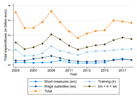
(a) Total expenditures

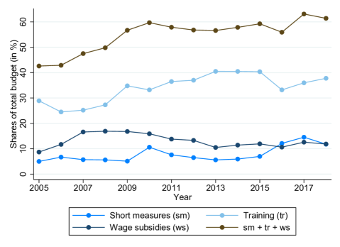
(b) Expenditure shares

Notes: Panel (a) plots the German expenditures for ALMP (discretionary measures) in billion euro. Panel (b) plots the corresponding expenditure shares by program type. Short measures (sm), training (tr), wages subsidies (ws). Source: https://statistik.arbeitsagentur.de (accessed in June 2022).

Allocation of funds to policies.  Our identification strategy relies on the idea that labour markets do not perfectly coincide with employment agencies at which the decision of the local policy mix is made. This decision is shaped by a multi-layer process of budget distribution which we outline below (see also Blien and Hirschenauer, 2005; Yankova, 2010; Lechner et al., 2015; Wapler et al., 2018).

Every year, the Federal Employment Agency (FEA) decides on a global budget for all discretionary measures (see Figure 1) which is distributed to 10 regional headquarters and 156 local employment agencies. The rules for allocation are regulated in the Social Code IV (§71b) which states “the regional development of employment, the demand for labour, the type and extent of unemployment as well as the particular expenditure development in the preceding financial year are to be taken into account.” In practice, the distribution is done in three steps. First, a fixed proportion of the budget is allocated to East Germany. Second, the budgets for East and West Germany are distributed among the regional headquarters in the respective regions. Third, the regional headquarters decide on the funds for each employment agency.

While the FEA and the regional headquarters set some overall guidelines of for the use of different types of policies, local employment agencies have a great deal of autonomy in the ultimate allocation of the budget to specific programs. Program-specific budgets, policy objectives and guidelines are fixed at the agency level in the final quarter of every year for the respective forthcoming year. If the budget is exhausted, the corresponding measure can no longer be offered (Yankova, 2010). Unused funds can be transferred to the following year. At the beginning of every year, each agency additionally determines the type of training measures to be carried out in a educational target plan (Bildungszielplanung). The aim is to further align training offers with the demand on the labour market.

Reform of the employment agencies in 2012.  From 2012 to 2013 around two-thirds of employment agencies changed their regional area of responsibility. Agencies gave up parts of their territories to other agencies, absorbed parts of territories from other agencies, merged in their entirety or were newly created. The reform took place in three steps in July 2012, October 2012 and January 2013. Overall, around 21 percent of municipalities changed their agency and the total number of agencies was reduced from 178 to 156. Since then, all agency borders correspond with district borders. Similar to the pre-reform period, new agencies are primarily defined as administrative and not functional areas (Hirschenauer, 2013).

3 What Macroeconomic Effects do we Expect?

A traditional motivation for ALMP has been to improve the matching process in the labour market and to reduce unemployment. From a theoretical point of view, these policies can have ambiguous effects on aggregate labour market outcomes (see e.g. Calmfors, 1994; Calmfors et al., 2002 and Layard et al., 2005 for seminal discussions). They might affect matching efficiency, productivity, job competition as well as job creation and destruction, in part through wage-setting and labour demand incentives. Positive effects on participants may be offset by negative externalities on non-participants such as substitution and displacement effects (Calmfors, 1994). Substitution effects occur when ALMP induce employers to hire from the stock of program participants instead of from the stock of non-participants do due to a change in relative labour costs. Displacement effects are closely related and refer to a crowding out of regular labour demand. Furthermore, the effectiveness of the policies might be compromised by deadweight effects. They arise if employers would have hired program participants even in absence of the measure.

In what follows, we consider each program separately and discuss expected net effects on employment, which is the focus of our analysis. In doing so, we take program-specific unintended effects into account. Deadweight losses and substitution effects are likely to affect all programs under consideration, while displacement are particularly relevant for wage subsidies. Our discussion will be guided by existing empirical evidence on the impact of ALMP at the individual level and the developments in labour demand. For the past decades, pronounced changes in labour demand for different jobs and skills have been documented globally (for Germany, see e.g. Hutter and Weber, 2021; Dustmann et al., 2009). In particular, so-called skill-biased technological change shifted demand towards (high) skilled labour (Acemoglu and Autor, 2011) and routine-biased technological change towards non-routine work (Autor and Dorn, 2013; Autor et al., 2015). These trends could have important implications for the effectiveness of the programs we study.

Short measures primarily aim at reducing frictional unemployment by improving matching efficiency in the market. Specifically, their objective is to remove information asymmetries regarding suitable vacancies, and to improve workers’ job search skills and search efficiency. If unemployment is characterised by structural mismatches due to an increasing demand for high-skilled and non-routine labour, short measures are unlikely to overcome them. The literature evaluating short measures in the 1990s and early 2000s in Germany, has found no or only small effects of these programs on individual employment (Wunsch and Lechner, 2008; Wunsch, 2013). The programs are more effective after a period of unsuccessful job-search (Biewen et al., 2014; Osikominu, 2013), if they have a vocational training component (Fitzenberger et al., 2013) or are executed in firms (Kopf, 2013; Gordo and Wolff, 2011; Stephan and Pahnke, 2011). Lock-in effects are short but the programs are not very successful in increasing employment stability and earnings in the long run (Osikominu, 2013, 2021). Considering the at most minor employment effects at the individual level, we might also not expect large effects in the aggregate, especially if only a small part of unemployment is frictional.

Training programs aim at reducing skill mismatch in the labour market by improving the occupational skills of jobseekers and adapting their qualifications to requirements of vacancies. They are expected to counteract human capital depreciation and to improve the match quality between workers and firms. These programs have been shown to reduce the search intensity of participants and to have considerable lock-in effects in the short run (Fitzenberger et al., 2008; Lechner et al., 2011; Biewen et al., 2014). How this affects the aggregate unemployment rate in the short run is unclear from a theoretical point of view. On the one hand, it might increase if the employment probability of non-participants remains unaffected. On the other hand, non-participants could benefit from less competition for the same stock of job vacancies, which could increase exits from unemployment in turn. In the long run, training programs have been shown to effectively increase individual employment (Card et al., 2018; Lechner et al., 2011; Biewen et al., 2014). They are thus likely to generate positive employment effects in the aggregate, unless hiring of participants comes at the expense of non-participants or incumbent workers.

Aggregate employment effects may differ for low-skilled and high-skilled workers and they may also depend on the presence of skill mismatch and labour market tightness. If targeted well, training programs can overcome structural mismatch and remove potential labour shortages. A shift in the workforce towards more skilled workers could then lead to positive employment effects for both the high-skilled and the low-skilled. Low-skilled workers might benefit if the competition in the low-skilled market gets smaller. However, it is also possible that public training crowds out firm investments in training. If firms do not find workers with suitable skills on the market and the gains from filling a vacancy are sufficiently large, they might turn to workers with insufficient skills, which the firms train themselves to obtain the missing skills. The availability of public training makes these investments unnecessary while the corresponding vacancies would still be filled. However, the reduction in hiring costs may additionally incentivise job creation. In the absence of skill mismatch or if training programs are poorly matching labour demand, aggregate employment effects are more ambiguous. The programs might change the composition of the labour force by increasing the proportion of high-skilled workers relative to the proportion of low-skilled. This might lower the bargaining power of the high-skilled and put downward pressure on their wages (Pissarides, 2000; Mortensen and Pissarides, 1994). Furthermore, it might affect job creation and lead firms to hire trained in the place of untrained jobseekers. Such substitution effects might be aggravated if the stock of available vacancies is limited and smaller than the stock of jobseekers.

Wage subsidies have the objective of reducing barriers to hiring by acting as a screening device for employers and reducing information asymmetries. They also aim at increasing participants’ labour market attachment and productivity through on-the-job training. With that, they are an alternative to formal training to counteract the devaluation of human capital and to reduce the mismatch between skill supply and demand. The literature evaluating wage subsidies in Germany found large positive effects on unsubsidised employment at the individual level (see Wolff and Stephan (2013) for a review). On aggregate, wage subsidies are expected to generate positive employment effects. In a static labour demand framework, wage subsidies reduce employer’s labour costs and are expected to shift the labour demand curve upwards, thereby increasing employment and wages (Bell et al., 1999). In the search and matching framework they are expected to reduce hiring frictions and thereby increase matching efficiency (Pissarides, 2000). Furthermore, they are likely to increase job creation by lowering hiring and wage costs in the short run. If successful, they can achieve long-term integration of jobseekers into unsubsidised employment through higher productivity of workers.

However, unintended effects might attenuate the overall effectiveness of these programs. In particular, displacement effects are an often discussed risk for wage subsidies (Calmfors et al., 2002; Dahlberg and Forslund, 2005). Firms might hire subsidised workers but jobs might be crowded out elsewhere in the economy (Calmfors and Skedinger, 1995). This might happen at the expense of other jobseekers as regular jobs are replaced with subsidized jobs. Furthermore, wage subsidies could depress the overall wage-level in the types of jobs that are subsidized. Overall, negative externalities depend largely on the exact design of the subsidies. A careful targeting to vulnerable groups of jobseekers with poor employment prospects as well as a mandatory period of employment after the subsidy runs out can attenuate unintended effects.

In summary, all three programs might generate positive effects on aggregate employment. The net effects will depend on their effectiveness in increasing employment prospects of the participants themselves and their negative externalities on non-participants through displacement and substitution effects. Furthermore, we might not expect the same aggregate effects for all segments of the labour market. On the one hand, there is substantial evidence for heterogenity in the effectiveness of the programs at the individual level (Card et al., 2018; McCall et al., 2016). On the other hand, not all workers might be equally affected by potential negative externalities. Low-skilled or medium-skilled workers who do not obtain wage subsidies, for example might suffer more from displacement effects than high-skilled workers.

4 Empirical Strategy

In this section we first introduce the general idea of our identification strategy and discuss the identifying assumptions. Second, we describe how we define labour markets and instrumental variables. Third, introduce the main sample restrictions for which the identifying assumptions are most likely fulfilled. Fourth, we present the data and finally our estimation method.

4.1 Exploiting Incomplete Overlap for Identification

4.1.1 General Idea

The endogeneity problem in macroeconomic evaluation studies of ALMP results from policies and aggregate labour market outcomes being determined simultaneously. As outlined in Section 2, in Germany regional labour market conditions determine policy implementation, which in turn determines regional labour market conditions. We propose a novel empirical strategy to overcome this problem. We estimate aggregate effects at the local labour market level and exploit the incomplete overlap of labour markets and administrative units that decide on the use of ALMP (in our context employment agencies, referred to as agencies in what follows). In contrast to the agencies whose borders evolved historically (Kropp and Schwengler, 2012), labour markets reflect spatial aspects of economic activity. They are functional regions that are spatially bounded by places of work and residency. We define such markets for Germany following (Tolbert and Sizer, 1996) based on home-to-work commuting flows between municipalities.

We find that labour markets are not perfectly coinciding with agencies and exploit the imperfect overlap of borders as source of exogenous variation. The idea is illustrated in Figure 2 for an exemplary labour market. The blue circle represents one labour market, which overlaps with four agencies (LEA1, LEA2, LEA3, LEA4). We are interested in measuring the effects of the policies implemented in this labour market, e.g. on the aggregate unemployment rate there. The policies might be in part endogenously determined by the labour market conditions in the blue area. To eliminate endogeneity, we instrument the policy take-up in the labour market with the policy take-up in the municipalities in the white areas outside the blue circle of the three employment agencies that partially overlap with the blue circle (LEA1, LEA2, LEA3). We define this area as instrument area. We argue that the policies in the white areas are correlated with the policies deployed in the market but exogenous to the labour market outcomes there, once we condition on the characteristics of the market.

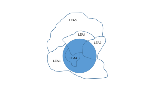
Figure 2: Illustration of the Identification Strategy

4.1.2 Identifying Assumptions

For this approach to be valid, we need to make two main identifying assumptions. First, we assume that there are no spillovers across labour markets and across areas considered for instrumentation. To lend support to this assumption, we base our analysis on self-contained labour markets that do not overlap (meaning little commuting flows between the markets).

Second, we assume that the policy use in the municipalities outside the labour market is correlated with policy use in the labour market, but exogenous to the outcome variables of interest, such as the unemployment rate and employment rate, given the characteristics of the market. This assumption consists of two parts: First, the instruments need to be relevant, i.e. there needs to be some correlation in the policy take-up in the labour markets and in the instrument areas. Second, the instruments need to be exogenous, i.e. there is no direct effect of the policy use in the instrument areas on the labour market outcomes in a labour market after controlling for the characteristics of the market. Furthermore, the instruments need to be uncorrelated with any other determinants of the labour market outcomes.

In order to assess the validity of the instruments, we need to understand how the policy mix in each labour market and agency is determined. Recall that each agency has discretionary power over how to allocate their budget to different policies (see Section 2). Policies implemented in a labour market are thus a mix of the policy making decisions of all overlapping agencies. The exogeneity of the instruments is coming from two sources. First, we claim that the strategies of the agencies are not only related to labour market conditions but also reflect different policy preferences and management styles (Fertig et al., 2006a). Second, the policies implemented in each labour market depend to a large extent on economic conditions and the composition of the labour force in regional jurisdictions of the overlapping agencies that lie outside the market. These conditions are likely to differ from the ones in the market, since the labour market situation is likely to change at the borders of self-contained labour markets. The exogeneity assumption is thus more likely to be valid i) if several agencies overlap with a labour market and we have more variation in policy styles, ii) if the labour force in the labour market represents only a small share of the labour force in the overlapping agencies, i.e. the agencies’ policy mix is more likely to be determined by conditions outside of the local labour market, iii) if we are able to characterize the economic situation in the labour market well.

Instrument relevance is based on the idea that there is some similarity in the policies implemented in the entire jurisdiction of the agency. If agencies follow a particular strategy independent of the economic conditions and composition of jobseekers in their area of responsibility, e.g. have a strong preference for training programs, this strategy will be reflected in the municipalities inside and outside of the labour market. The policy use in the instrument area and the labour market will then be correlated. This should be true independent of how large the labour force in the market is compared to the labour force in all partially overlapping agencies. Jointly, all overlapping agencies determine the policies deployed in the market. Nevertheless, it is likely that the relevance assumption is more likely to hold if the overlap between single agencies and the labour market is not too small.

4.2 Definition of Local Labour Markets

We construct local labour markets based on commuting flows between all German municipalities in 2016 provided by the German Federal Employment Agency (Bundesagentur für Arbeit). Commuters are captured by employment statistics and comprise all employees that were subject to social security contributions on June 30 and whose place of work is different from their place of residence. The employment statistics further allow us to derive the resident labour force (RLF), i.e. the sum of all employees that live in a region and local labour force (LLF), i.e. the sum of all employees that work in a region for each municipality. We complement these data with driving distances between all German municipalities from the Leibniz Institute for Economic Research (RWI). These distances record the driving time by car (in seconds) between the population centers of each municipality for the year 2016.

We follow the clustering approach developed by Tolbert and Killian (1987) and Tolbert and Sizer (1996) who derive commuting zones based on county to county commuting flows in the US. Compared to US counties, German municipalities are substantially smaller and vary considerably more in size. Since this heterogeneity negatively affects the performance of the clustering algorithm, we first create a more homogeneous database by aggregating the approximately 11000 municipalities into fewer municipality regions. For this, we follow an approach similar to Kropp and Schwengler (2016) and merge sparsely populated municipalities that are close to each other. We calculate a fusion coefficient $F_{ij}$ for every municipality pair $(i,j)$ according to the formula $F_{ij}=distance_{i,j}^{2}*(RLF_{i}+RLF_{j})$ which is based on the squared distance between the municipalities and their RLF.

We then aggregate adjacent municipalities using a hierarchical clustering algorithm with complete linkage. This algorithm first merges the two municipalities with the lowest fusion coefficient and then subsequently adds up similar clusters by considering the largest dissimilarity between the municipalities in two clusters. We generate three different versions of pre-processed data stopping the clustering at 5000, 6500 and 7500 municipality regions. This gives us the chance to check the sensitivity of our results to this first aggregation step. This first step is characterised by a trade-off between homogeneity and size. A higher number of municipality regions results in more homogeneous regions but also in a higher aggregation level as input for the definition of commuting zones.

In a second step, we cluster the municipality regions based on the strength of commuting ties between them, starting with 5000. First, we calculate a proportional commuting measure for each pair of municipality regions as proposed by Tolbert and Killian (1987):

$$S_{ij}=\frac{(P_{ij}+P_{ji})}{min(RLF_{j},RLF_{i})},$$

where $P_{ij}$ denotes the commuting flows from municipality region $i$ to $j$ and $P_{ji}$ the commuting flows in the other direction. The denominator corresponds to the minimum of the resident labour force in region$i$ or $j$. This measure captures the commuting relationship between two regions with respect to the smaller of the two regions and has a large value if the commuting ties are strong. We then collect these similarity measures $S_{ij}$ in a symmetric matrix and set the diagonals to 0. Since the clustering algorithm that we apply requires a dissimilarity measure, we derive: $D_{ij}=1-S_{ij}$.

We use a hierarchical clustering algorithm with average linkage and cluster municipality regions with strong commuting ties bottom up until an average between cluster distance of $c$ is reached. Since there is no clear ex-ante guideline of where to stop the clustering, we run the algorithm several times and stop at different values of $c\in\{0.98,0.99,0.991,0.993,0.995,0.997,0.999\}$. For every stopping value we obtain a different number of clusters (or labour markets) with higher values resulting in larger and fewer regions. Tolbert and Sizer (1996) choose an average cluster distance of 0.98 as stopping rule, which we take as minimum value. Given the smaller size of underlying municipality regions, this cut-off leads to a total of 462 labour markets of a relatively small size (average RLF equal to 67700). The maximum stopping value that we choose lies at 0.999 and results in 59 labour markets with an average RLF equal to 530000). We store the number of clusters corresponding to the respective stopping values and repeat the clustering exercise based on 6000 and 7500 municipality regions. In contrast to the first round based on 5000 municipality regions, we now use the stored total number of clusters as stopping rule in order to obtain the same number of labour markets for each underlying number of municipality regions. In the following, we will present the results obtained based on 6000 municipality regions. As described in Appendix A.1.1, the characteristics of the resulting labour markets are not very sensitive to this first aggregation step.

Characterizing the labour market definitions  Table 1 gives an overview of our labour market definitions based on different stopping values (column 2). Column (3) reports the number of labour markets that we obtain, column (4) the average RLF in the markets and columns (5)-(9) describe two measures of self-containment. The commuter ratio (CR) in column (5) measures the share of all commuters between labour markets as percent of the total labour force. This value will be small if labour markets are self-contained and there is little commuting across borders. Columns (6)-(9) show the average, the standard deviation, the minimum and maximum of the so-called employment self-containment ratio (ESC) introduced by Laan and Schalke (2001). The ESC measures the share of people living in a region who also work there.

Table 1: Labour Market Definitions

(1)	(2)	(3)	(4)	(5)	(6)	(7)	(8)	(9)
Def.	Cut-off	LLM (N)	RLF (mean)	CR	ESC (mean)	ESC (sd)	ESC (min)	ESC(max)
1	0.98	462	67652.63	20.22	65.77	16.46	11.11	98.27
2	0.99	274	114071.22	15.91	74.03	13.07	11.11	98.27
3	0.991	251	124523.96	14.89	75.50	12.24	11.11	98.27
4	0.992	229	136486.96	14.08	76.63	11.75	11.11	98.27
5	0.993	209	149547.91	13.57	78.03	10.44	16.56	98.27
6	0.994	187	167141.79	12.78	79.11	10.43	16.56	98.27
7	0.995	162	192935.27	12.06	80.71	8.34	45.88	98.27
8	0.996	138	226489.23	11.10	82.35	7.78	54.43	98.27
9	0.997	121	258310.03	10.35	83.41	7.61	54.43	98.27
10	0.998	92	339733.85	8.21	86.39	5.44	65.34	98.27
11	0.999	59	529754.47	5.83	89.68	3.81	76.56	98.27

Both measures of self-containment increase with higher stopping values. Labour market definitions with fewer and larger labour markets are characterised by a higher ESC and a lower commuting ratio. All definitions are characterised by a high level of variation in self-containment. The heterogeneity is less pronounced for higher cut-off values. Based on this evidence, we can conclude that labour market definitions based on higher stopping values are thus more likely to represent closed, functional entities between which regional spillovers are less likely and which satisfy the identifying assumptions best. The final choice of definition depends on the imperfect overlap of labour markets with agencies, which we discuss in the next section.

Appendix Figure A.3 shows a map of the resulting 162 labour markets obtained by the clustering approach described above, based on the cut-off value of 0.995 (our preferred version). Labour markets are shown as coloured areas, the borders of employment agencies (as from 2013) through black solid lines. Labour markets and employment agencies are relatively heterogeneous in size and reflect the distribution of agglomerations in Germany. Comparatively small employment agencies usually represent rather large cities. Often these cities are the center of a large labour market, as for example in the case of Berlin.

Comparison to existing definitions.  There exist a number of local labour market definitions based on home-to-work commuting flows for Germany, e.g. 50 labour markets by Kropp and Schwengler (2011a, 2016) or 141 labour markets by Kosfeld and Werner (2012). Two additional definitions for Germany that are frequently used are the 258 labour market regions of the Joint Task of the Federal Government and the federal states dedicated to the "Improvement of Regional Economic Structure" (GRW) and the 96 spatial planning units by the Federal Institute for Research on Building, Urban Affairs and Spatial Development (BBSR).

However, none of the existing definitions are suitable for our methodological approach. The majority is based on aggregations of around 400 districts. Compared to municipalities, districts constitute relatively highly aggregated administrative areas and are thus not able to capture the subtleties in spatial structures that we want to exploit. The resulting labour markets are likely to perfectly overlap with employment agencies. Only one labour market definition (Kropp and Schwengler, 2011a, 2016) is based on commuting flows between municipalities but it contains too few and too large regions for our purposes. We compare our labour market definitions to these established definitions of local labour markets in Appendix A.1.5 and find that our approach results in qualitatively comparable labour markets in terms of self-containment.

4.3 Instrument Areas and Sample Selection

We define an instrument area for each labour market. It comprises those municipalities that are outside of a labour market but within the jurisdiction of agencies that partially overlap with the market. The policy use in this area is then jointly considered for the construction of the instruments. As outlined in Section 4.1.2, the instruments are more likely to be valid if the overlap between a labour market and the employment agencies meets certain criteria. For our main analysis we impose the following restrictions. They have to hold for the entire observation window: First, a labour market should overlap with at least two agencies. Second, the resident labour force (RLF) in the market should not constitute more than 50% of the total RLF in all agencies that partially overlap with the market ($s_{tot}=RLF_{LLM}/\sum_{j}RLF_{LEA,j}<0.5$). This ensures that the labour market situation in the labour market does not drive the policy mix in overlapping agencies too strongly and that the policy mix deployed in the instrument areas is likely to represent an exogenous source of variation. For the main analysis, we do not impose a minimum criterion on the overlap. The reasoning behind this is that instrument relevance can be tested and that it should not depend on how large the instrument area is in relation to the size of the market. But we set restrictions on the overlap of single agencies and the labour market in a robustness check.

In order to guide the choice of a labour market definition, we investigate how imposing these restrictions affects both sample size and the number of overlapping agencies across definitions. Figure 3 (a) plots the number of labour markets as a function of the average level of self-containment. The definitions are based on different stopping values in the clustering step. The light blue line shows the original number of markets, the mid blue line plots the same relationship after conditioning on the overlap criteria for our main specification. Consistent with what we discussed in Section 4.2, higher stopping values result in fewer labour markets with a higher level of self-containment. Restricting overlap reduces the number of labour markets that remain in the sample across all labour market definitions. The reduction is more substantial for the definitions based on larger stopping values. Figure 3 (b) shows that the average number of overlapping agencies is increasing with larger and more self-contained labour markets, i.e. higher stopping values. An increase in self-containment from about 75 to 85% is associated with only a moderate increase in the number of overlapping agencies of about 0.5.

Figure 3: Labour Market Definitions, Overlap Restrictions and Self-containment

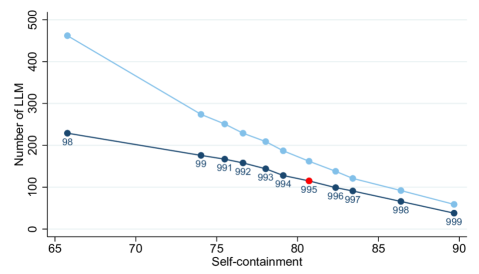
(a) Number of labour markets by definition

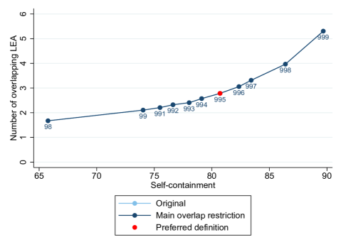
(b) Average number of overlapping agencies

Notes: Panel (a) plots the number of labour markets, panel (b) the average number of overlapping employment agencies for different levels of self-containment. The original number of labour markets is shown in light blue, the number of markets (and overlapping agencies) after imposing the main overlap restrictions in dark blue. Each dot represents a labour market definition based on a specific stopping value in the clustering step. Our preferred definition is marked in red.

This illustrates that we face a trade-off between the representativeness of the analysis and a clean identification strategy. Our preferred labour market definition should guarantee a sufficient level of representativeness while maximizing the self-containment of the markets as well as the number of overlapping agencies. The labour market definition that is based on the stopping value of 0.995 achieves this objective. After imposing our main sample restrictions, we obtain an average level of self-containment above 80%, while maintaining a total number of 115 labour markets. This corresponds to 71 % of the original number of labour markets and comprises 64% of the total labour force in Germany (in 2016). The average number of overlapping agencies is larger than two. Appendix Figure A.5 shows how the labour markets are distributed geographically. Notice that imposing restrictions on the overlap leads to the exclusion of several labour markets around big cities, such as Berlin and Munich. Given that the labour market situation in these markets is likely to be strongly determined by the respective cities, a clean identification of effects in these markets is difficult. We test the sensitivity of our results to the choice of different labour market definitions and overlap criteria in Section 6.

4.4 Data

For the main analysis we rely on social security records for the years 2000 to 2018 from the Integrated Employment Biographies (IEB) provided by the Institute of Employment Research (IAB) in Germany. Jointly, it covers the universe of program participants in ALMP, a 10% random sample of unemployed individuals and a 2% random sample of employed individuals. For all of these individuals we observe the labour market histories from 1994 to 2018 with daily accuracy coming from the integrated employment biographies (IEB).

From these individual-level data we construct a panel dataset of labour markets at the quarterly level. It contains aggregate endogenous policy and instrumental variables, a set of variables characterizing the workforce in the labour market and aggregate labour market outcomes. We restrict our attention to individuals who are between 20 and 64 years old, since we are interested in macroeconomic effects for the main working population (excluding students and pensioners). The sample of unemployed is used to characterise the unemployed workforce in a labour market and to define aggregate labour market outcomes. The sample of employed is used for the characterization of the employed workforce and aggregate labour market outcomes. The variables measuring the use of ALMP are based on the full population of program participants. We follow the literature (e.g. Calmfors et al., 2002; Wapler et al., 2018) and measure the policy variables as so-called accommodation rates. They are defined as the share of participants in a specific program among the jobseekers drawing UI benefits in a labour market. For the instrumental variables, we construct the same shares by dividing the sum of program participants in all instrument areas of a labour market by the total number of jobseekers on UI in the same areas. Our main outcomes of interest are the aggregate unemployment rate (share of UI recipients in the RLF), the unsubsidised employment rate (the share of workers in unsubsidised employment in the RLF), the rate of welfare recipients (the share of unemployed workers receiving welfare benefits in the RLF) and the rate of employed workers on benefits (the share of workers with small jobs that receive UI or welfare benefits). Since not all segments of the workforce might be similarly affected by ALMP, we also consider the corresponding rates for different sub-populations such as females, males, individuals below 30, above 50, low, medium and high-skilled.

Censoring.  For data protection reasons, we are obliged to censor quantities based on less than three observations (excluding zero). This entails a significant share of missing values in some of the variables, in particular for small labour markets. We pursue different strategies to deal with the missing values. First, our main sample restrictions naturally lead to the exclusion of small labour markets. Additionally, they ensure that no outcome variables are censored in the final dataset. Second, for all censored control variables characterizing the employed and unemployed workforce, we replace the original variable with 0 and create separate variables flagging censored values. For all variables measuring program participation, we impute censored counts of program participants with the value one. This yields a lower bound on the true count of program participants but the margin of error remains small.

Description of the final dataset.  Based on our preferred definition of labour markets and main sample restriction, we obtain a balanced panel of 115 labour markets which we observe for 52 quarters, from the first quarter of 2005 to the first quarter of 2018. We use the period from 2000 to 2004 merely for the construction of lagged variables in our dynamic panel data model (see Section 4.5). Appendix tables A.4 and A.5 present summary statistics for all outcome, policy and control variables. Figure 4 shows the variation of the main outcome variables over time, Figure 5 the variation of the policy variables. The solid line depicts the sample average in each quarter and the grey area the corresponding standard deviation.

The average unemployment rate (Figure 4(a)) is decreasing from a level of 6 to 2% over the time period that we consider, with a temporary increase in the years around the great recession. It is characterised by strong seasonal fluctuations which are driven by a high number of inflows into unemployment at the beginning of each year. The employment rate (Figure 4(b)) is mirroring the trends in unemployment and increases from a level of 82% to 89% over time. The rate of welfare recipients (Figure 4(c)) and employed workers (Figure 4(d)) on benefits increases from 2005 to 2006 and follows a slight downward trend thereafter. The standard deviation is smallest for the unemployment rate and comparatively large for the other outcomes, suggesting that there is substantial variation in the share of employed, welfare recipients and employed workers on benefits across labour markets.

The seasonality in the unemployment rate is reflected in the accommodation rates of program participants. Apart from these fluctuations, the shares follow trends that are similar to the expenditure shares presented in Figure 1. The average share of unemployed in training (Figure 5(a)) increases over time, with a slight drop in 2012. This drop can be explained by a larger number of individuals leaving the stock of participants who started their program during the years of the great recession. Further, the average share of unemployed in short measures (Figure 5(b)) follows an upward trend. Additionally, it jumped from 5 to 20% with the change in legislation in 2009. Wage subsidies (Figure 5(c)) were more heavily used around the years of the great recession and remained at a level of around 5% after 2013. As Appendix Figure A.5 shows, there is also substantial variation in the policy use and across labour markets. Wage subsidies, for example, were more heavily deployed in East Germany. This is where the unemployment rate was highest on average during our observation period.

Figure 4: Variation in Outcomes over Time

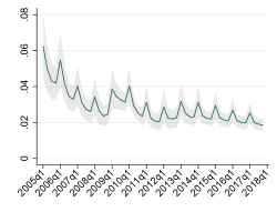
(a) Unemployment rate

(b) Unsubsidised employment rate

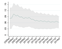
(c) Rate of welfare recipients

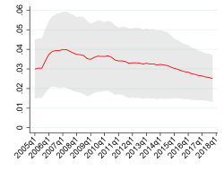
(d) Rate of employed workers on benefits

Notes: The figures depict the average quarterly variation of the outcomes (a) unemployment rate, (b) unsubsidised employment rate, (c) rate of welfare recipients (d) rate of employed workers on benefits for the period 2005 to 2018. The standard deviation is depicted as grey area.

Figure 5: Variation in Programs over Time

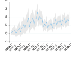
(a) Training

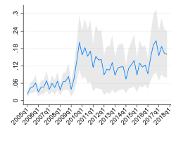
(b) Short measures

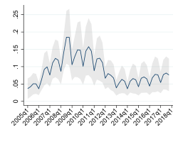
(c) Wage subsidies

Notes: The figures depict the average quarterly variation of the three programs (a) training, (b) short measures and (c) wage subsidies for the period 2005 to 2018. The standard deviation is depicted as grey area.

4.5 Estimation

To implement our empirical strategy, we rely on an estimation method that accounts for the dynamic nature of the policy effect on the outcome. The ALMP that we study range from a few weeks up to 3 years. We thus expect the effects to occur with some time lag and to potentially accumulate over time. Moreover, programs might affect intermediate outcomes. We estimate the following autoregressive distributed lag model ARDL(1,q):

$$\Delta y_{it}=\theta\Delta y_{i,t-1}+\sum_{m=1}^{M}\sum_{j=0}^{q}\phi_{j}^{m}\Delta X_{i,t-j}^{m}+\gamma W_{i,t-q}+\mu_{t}+\Delta\epsilon_{it},$$ (1)

where $\Delta y_{it}=y_{it}-y_{i,t-4}$ is the yearly change in the outcome $y$ in market $i$ and quarter $t$. This change is regressed on the yearly change in the lagged outcome ($\Delta y_{i,t-1}$) and the yearly changes in the endogenous accommodation rates for the $M=3$ programs ($\Delta X_{i,t}^{m},\ldots,\Delta X_{i,t-q}^{m}$). In our main specification accommodation rates are included with $q=6$ lags.

We estimate the model in year differences to deal with integrated time series and serial correlation in the residuals. This is necessary since our outcome and policy variables are characterised by strong yearly fluctuations (see Figures 4 and 5 ). At the same time, we directly difference out labour market fixed effects and thereby all aggregate effects that are market specific and time-constant. A vector of exogenous labour market characteristics measured in $t-q$ ($W_{i,t-q}$) additionally takes care of possible changes in the labour market composition over time. It includes the gender, age, nationality, education, training and industry composition of the employed and unemployed workforce, the share of welfare recipients (as percent of the RLF) and the shares of participants in other ALMP. Finally, quarter-year fixed effects ($\mu_{t}$) control for aggregate time-trends such as the business cycle. Jointly this rich set of controls makes our instruments conditionally exogenous. For identification, we exploit the residual variation in policy use within labour markets and corresponding instrument areas.

The coefficient $\phi_{0}^{m}$ measures the contemporaneous (or short-term) effect of an increase in the share of program participants in program $m$ relative to all jobseekers on aggregate labour market outcomes. The long-run effect is given by $\sum_{j=0}^{q}\phi_{j}^{m}/(1-\theta)$. We also derive the marginal and cumulative marginal effects of a permanent increase in the shares of unemployed in a specific program type for different quarters. The effects can be interpreted as aggregate effects of an increase in the intensity of a specific ALMP. They measure the net effect of these policies on labour market outcomes by jointly considering the direct effect on participants and possible positive or negative spillover effects on non-participants.

We estimate the model both using OLS and two-stage least-squares (2SLS). For the latter, we instrument the endogenous variables $\Delta X_{i,t}^{m}\ldots,\Delta X_{i,t-q}^{m}$ with the same set of instruments $\Delta Z_{i,t}^{m},\ldots,\Delta Z_{i,t-q}^{m}$. $\Delta Z_{i,t}^{m}$ that measure the accommodation rates in the instrument regions. Our instrumental variable model is just-identified, with 21 endogenous regressors and instruments in our main specification of lag order 6. We do not instrument for the lagged dependent variable but argue that any bias from $Cov(\Delta y_{i,t-1},\Delta\epsilon_{it})\neq 0$ would be negligible since we have a long time series with $T>50$. We assess this potential bias in a robustness check by comparing our results to a distributed lag model that does not include a lagged depended variable. The results are qualitatively comparable across models. We estimate standard errors using a cross-sectional bootstrap procedure where we re-sample entire labour markets.

5 Results

5.1 First Stage

Before turning to the results, we test whether our proposed instruments are relevant. In a single endogenous variable model it is common to use the standard first-stage F-statistic to test for weakness of the instruments. Since we instrument for 21 endogenous variables in our model, this statistic is no longer sufficient. Thus, we perform two alternative tests instead, which were developed for the setting with multiple endogenous variables. Sanderson and Windmeijer (2016) propose a test that is constructed for individual endogenous regressors by partialling-out linear projections of the remaining endogenous regressors. A similar approach by Angrist and Pischke (2009) derives conditional F-statistics by replacing other endogenous variables by their reduced form prediction. The corresponding F-statistics and p-values for the first-stage regressions are reported in Table 2 exemplarily for the model including the lagged dependent unemployment rate. We find large and highly significant F-statistics for all endogenous policy variables suggesting that instrument relevance is given. The F-statistics are highest for wage subsidies.

5.2 Effects on Aggregate Labour Market Outcomes

We present our main results for the unemployment rate and the unsubsidised employment rate in Table 5.3 and for the rate of welfare recipients and the rate of employed workers that receive state benefits (the so-called working poor) in Table 5.3. Columns (1) to (3) show the effects, standard errors and p-values based on the estimation of the ARDL model using OLS. Columns (4) to (6) show the same quantities estimated by 2SLS. The tables present the short-term and long-term effects of a ceteris paribus increase in the shares of participants in training, short measures and wage subsidies. The first row of each panel shows the coefficient on the lagged dependent variable. Figures 6 and 7 further inform about the dynamics behind the effects. They show the cumulative marginal effects on the labour market outcomes up to 12 quarters after an increase in the shares of program participants.

Table 2: First Stage - Unemployment Rate

	SW F-stat	SW p-val	AP F-stat	AP p-val
AR training	108.26	0.000	123.08	0.000
AR training (lag 1)	79.51	0.000	142.96	0.000
AR training (lag 2)	91.79	0.000	97.79	0.000
AR training (lag 3)	85.31	0.000	69.23	0.000
AR training (lag 4)	83.68	0.000	97.21	0.000
AR training (lag 5)	72.93	0.000	98.37	0.000
AR training (lag 6)	107.81	0.000	265.05	0.000
AR short measures	61.26	0.000	364.19	0.000
AR short measures (lag 1)	56.50	0.000	146.69	0.000
AR short measures (lag 2)	83.31	0.000	155.23	0.000
AR short measures (lag 3)	47.92	0.000	143.34	0.000
AR short measures (lag 4)	63.36	0.000	146.18	0.000
AR short measures (lag 5)	59.32	0.000	150.48	0.000
AR short measures (lag 6)	67.61	0.000	225.94	0.000
AR wage subsidies	98.99	0.000	398.67	0.000
AR wage subsidies (lag 1)	102.54	0.000	418.28	0.000
AR wage subsidies (lag 2)	95.11	0.000	187.66	0.000
AR wage subsidies (lag 3)	103.43	0.000	245.01	0.000
AR wage subsidies (lag 4)	107.53	0.000	211.31	0.000
AR wage subsidies (lag 5)	83.56	0.000	225.16	0.000
AR wage subsidies (lag 6)	120.17	0.000	490.66	0.000

Notes: The table reports two types of diagnostic test of the first stage for the 21 excluded instruments for the model including the lagged dependent unemployment rate. Each line refers to a separate first-stage regression for the respective accommodation rate (AR). The first two columns show the Sanderson-Windmeijer (2016) F statistics (SW F-stat) and p-values. Columns 3 and 4 the Angrist-Pischke (2009) F-statistics and p-values (AP F-stat).

In both estimation methods, we find the lagged dependent variable to be significant. The estimates range from 0.63 to 0.7 and are lowest for the the unemployment rate. This suggests that there is indeed a temporal adjustment process. Based on the OLS estimation we find small negative long-term effects of all programs on the unemployment rate, the rate of welfare recipients and the rate of employed workers on benefits and a simultaneous positive effect on the employment rate. The effects are small in magnitude for short measures and training and larger for wage subsidies. The effects estimated by 2SLS are deviating in sign and magnitude, in particular for training and short measures. OLS seems to overestimate the effects of these policies on the employment rate. As expected, standard errors based on 2SLS are larger compared to the OLS model.

In the following, we only discuss the results based on the instrumental variables model. We do not find a significant effect of short measures on aggregate labour market outcomes. If anything, the results suggest that short measures slightly reduce the share of employed workers on benefits. For training we find no effects in the short run but a small marginally significant effect on the unemployment rate in the long run. The cumulative marginal effects in Figures 6 and 7 suggest that this effect starts to materialise after approximately four quarters. The employment rate does not increase. Instead, our results suggest that training reduces unemployment of UI recipients at the expense of unemployed welfare recipients, although the corresponding estimates in Table 5.3 are too imprecise for statistical significance. For wage subsidies we find a small negative short-term effect on the unemployment rate, which most likely picks up the effect of jobseekers moving out of unemployment and entering subsidised employment when starting this program. As can be seen from Figure 6, this negative effect only derives from the first quarter since the marginal effect on unemployment is zero and mostly positive thereafter. In the long run, wage subsidies have an economically meaningful and statistically significant positive effect on the employment rate. The unsubsidised employment rate increases by 2.9 percentage points for a 10 percentage point increase in the share of jobseekers (on UI) in wage subsidies. Of this increase, 80% is explained by a decrease in the rate of welfare recipients and 20% by a decrease in the rate of employed workers on benefits. Thus, wage subsidies increase employment, prevent long-term unemployment after exhaustion of UI and reduce the number of working poor.

Overall, our results are in line with our expectations in Section 3. First, we did not expect to find large aggregate effects for short measures, given that documented individual-level effects have been small. This was confirmed by our empirical analysis. Second, we find no evidence of an aggregate net effect of training programs on employment. Microeconometric studies document large lock-in effects for program participants in the short-term and positive employment effects in the long-term (McCall et al., 2016). Our results suggest that there are unintended effects on non-participants that are particularly likely if the number of vacancies that can be filled is limited and much lower than the number of jobseekers, which was the case in Germany in our observation period (Seele, 2018, Figure 1.1.) In the short run, firms might hire non-participants in place of program participants who are not available to the market during the program. In the long run, training participants may seem to find jobs at the expense of non-participants. Our results suggest that unemployed welfare recipients may suffer from these substitution effects. Third, the positive effects of wage subsidies on unsubsidised employment are in line with the effects that have been documented on the individual-level (see e.g. Stephan, 2010; Jaenichen and Stephan, 2011). This does not rule out the existence of displacement effects, but we find that positive employment effects dominate on the aggregate. This suggests that wage subsidies succeeded in creating new jobs and in increasing matching efficiency regarding existing jobs. A higher intensity of wage subsides does not lower the rate of jobseekers in UI but reduces the share of long-term unemployed on welfare and the share of workers that are stuck in precarious work. Thus, this program effectively prevents long-term dependence of jobseekers on state benefits.

5.3 Effects on Unemployment and Employment Rates for Different Segments of the Labour Market

In addition to looking at average outcomes for the entire labour market, we examine whether specific segments are differentially affected by ALMP. There are several reasons why such an analysis is interesting. First, the literature on individual-level effects of ALMP has documented substantial effect heterogeneity across participants with different characteristics. Regarding the gender of participants, females were found to benefit more both from training and wage subsidies (e.g. Card et al., 2018; Biewen et al., 2014; Kruppe and Lang, 2018). The evidence on heterogeneity with regard to age and skill levels is mixed (Card et al., 2018; Osikominu, 2013). Generally, jobseekers with relatively bad labour market prospects have been shown to benefit more from programs (Wunsch and Lechner, 2008; Cockx et al., 2019; Knaus et al., 2022).

This heterogeneity might also materialise at the regional level. Second, if negative externalities exist, they might not affect all individuals on the labour market equally. For instance, more vulnerable groups such as low-skilled workers are more likely to suffer from indirect effects. Finally, there is selectivity in the assignment of programs to jobseekers. If certain groups of jobseekers have no or less access to ALMP, they are unlikely to draw direct benefits from the programs but might be affected by indirect spillover effects.

Table 3: Effects on the Unemployment Rate and Unsubsidised Employment Rate

	OLS			2SLS
	(1)	(2)	(3)	(4)	(5)	(6)
Unemployment rate
	effect	se	p-val	effect	se	p-val
Lagged dependent variable	0.656	0.010	0.000	0.629	0.035	0.000
Training(st)	-0.017	0.002	0.000	0.000	0.012	0.989
Training(lt)	-0.010	0.005	0.032	-0.030	0.019	0.116
Short measures (st)	-0.007	0.001	0.000	0.002	0.009	0.780
Short measures (lt)	-0.006	0.003	0.022	-0.004	0.011	0.721
Wage subsidies (st)	-0.034	0.002	0.000	-0.030	0.010	0.003
Wage subsidies (lt)	-0.017	0.006	0.009	0.007	0.014	0.589

Unsubsidised employment rate    effect se p-val effect se p-val Lagged dependent variable 0.701 0.014 0.000 0.685 0.013 0.000 Training(st) 0.025 0.006 0.000 -0.009 0.030 0.759 Training(lt) 0.050 0.019 0.008 -0.022 0.092 0.811 Short measures (st) 0.004 0.004 0.240 -0.008 0.022 0.718 Short measures (lt) 0.025 0.011 0.032 0.003 0.042 0.945 Wage subsidies (st) 0.022 0.008 0.006 0.039 0.050 0.436 Wage subsidies (lt) 0.141 0.020 0.000 0.285 0.062 0.000 Quarter-Year FEs $\checkmark$ $\checkmark$ Additional Controls $\checkmark$ $\checkmark$ Observations 5980 5980 LLM 115 115 Notes: This table shows the coefficient on the lagged dependent variable, the short-term (st) and long-term (lt) effects of the three types of ALMP, i.e. training, short measures (SM) and wage subsdies (wagesub) on the unemployment rate (upper panel) and unsubsidised employment rate (lower panel). Columns (1)-(3) show the effects, standard errors (se) and p-values (p-val) for the OLS specification. Columns (4)-(6) show effects, standard errors and p-values for the IV specification. Program variables included with 6 lags, main sample restrictions. Standard errors obtained by a cross-sectional bootstrap (499 replications).

Table 4: Effects on the Rate of Welfare Recipients and Individuals in Precarious Work

Rate of employed workers on benefits    effect se p-val effect se p-val Lagged dependent variable 0.681 0.011 0.000 0.669 0.015 0.000 Training(st) 0.001 0.002 0.726 0.002 0.010 0.852 Training(lt) -0.012 0.006 0.047 -0.006 0.025 0.820 Short measures (st) 0.002 0.001 0.067 -0.001 0.007 0.915 Short measures (lt) -0.002 0.003 0.603 -0.017 0.011 0.105 Wage subsidies (st) 0.000 0.003 0.948 -0.004 0.012 0.761 Wage subsidies (lt) -0.047 0.007 0.000 -0.082 0.018 0.000 Quarter-Year FEs $\checkmark$ $\checkmark$ Additional Controls $\checkmark$ $\checkmark$ Observations 5980 5980 LLM 115 115 Notes: This table shows the coefficient on the lagged dependent variable, the short-term (st) and long-term (lt) effects of the three types of ALMP, i.e. training, short measures (SM) and wage subsdies (wagesub) on the rate of welfare recipients (upper panel) and rate of employed workers on benefits (lower panel). Columns (1)-(3) show the effects, standard errors (se) and p-values (p-val) for the OLS specification. Columns (4)-(6) show effects, standard errors and p-values for the IV specification. Program variables included with 6 lags, main sample restrictions. Standard errors obtained by a cross-sectional bootstrap (499 replications).

Figure 6: Cumulative Marginal Effects on the Unemployment Rate and Unsubsidised Employment Rate

Training

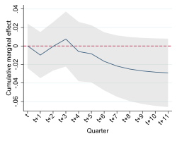
(a) Unemployment rate

Training

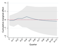
(b) Unsubsidised employment rate

Short measures

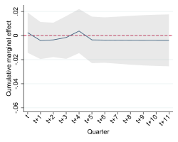
(c) Unemployment rate

Short measures

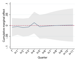
(d) Unsubsidised employment rate

Wage subsidies

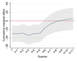
(e) Unemployment rate

Wage subsidies

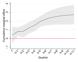
(f) Unsubsidised employment rate

Notes: These graphs show the marginal and cumulative marginal effects of the three types of ALMP, i.e. training, short measures and wage subsidies on the unemployment rate and unsubsidised employment rate by quarter. 95% confidence intervals are shown as grey areas. The effects are based on the ARDL model estimated by 2SLS. Program variables are included with 6 lags, main sample restrictions apply. Standard errors obtained by a cross-sectional bootstrap (499 replications).

Figure 7: Cumulative Effects on the Rate of Welfare Recipients and Employed Workers on Benefits

Training

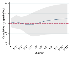
(a) Rate of welfare recipients

Training

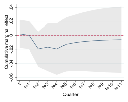
(b) Rate of employed workers on benefits

Short measures

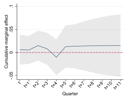
(c) Rate of welfare recipients

Short measures

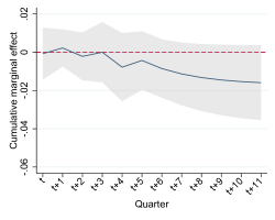
(d) Rate of employed workers on benefits

Wage subsidies

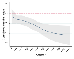
(e) Rate of welfare recipients

Wage subsidies

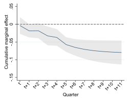
(f) Rate of employed workers on benefits

Notes: These graphs show the marginal and cumulative marginal effects of the three types of ALMP, i.e. training, short measures and wage subsidies on the rate of welfare recipients and rate of employed workers on benefits by quarter. 95% confidence intervals are shown as grey areas. The effects are based on the ARDL model estimated by 2SLS. Program variables are included with 6 lags, main sample restrictions apply. Standard errors are obtained by a cross-sectional bootstrap (499 replications).

Figures 8 and 9 depict the long-run effects of training, short measures and wage subsidies on the labour market outcomes of different subgroups. Appendix Figures A.6 to A.13 show the corresponding cumulative marginal effects on the unsubsidised employment and unemployment rates. Specifically, we consider males, females, workers of different ages (below the age of 30, ages 30 to 50 and above the age of 50) as well as low, medium and high-skilled workers. Similar to our control variables, we define low-skilled as workers without a vocational or academic degree, medium skilled workers as workers with a vocational degree and high-skilled workers as workers with an academic degree.

We find some suggestive evidence for heterogeneous aggregate effects across subgroups, even though the confidence intervals largely overlap. When differentiating by gender, the results suggest that males benefit more from training compared to females. While the effect on the unemployment rate is zero for females, it is negative for males. Nevertheless, the effect for males is small and not clearly reflected in a higher employment rate, while for females the estimates lean more towards negative effects on employment. Thus, the overall conclusions about training do not change but the net gains and losses show a tendency of being distributed unequally across gender. Moreover, the effect heterogeneity found at the individual level with more gains for females is not reflected in the aggregate. The same tendency is visible for short measures but the effects are mostly insignificant. If anything, men seem to benefit from short measures by being less dependent on welfare. In contrast, females seem to benefit more from wage subsidies in the long run, which is in line with the effect heterogeneity documented on the individual level.

With respect to age, we find relatively large and positive effects of training for workers above the age of 50 but not for younger workers. These workers experience a long-term decrease in their unemployment rate of around 0.10 percentage points, which is mirrored in a marginally significant increase in the employment rate and a decrease in the rate of employed workers on state benefits. Thus, we do find net benefits of training but only in this segment of the labour market. Also for wage subsidies the effects on the employment rates are higher for older workers. This age gradient is mirrored in lower rates of workers on welfare and a lower share of employed workers on benefits.

The effects on the labour market outcomes of different skill groups are very noisy. This is partially driven by the low shares of low and high-skilled individuals amongst the unemployed and employed in some labour markets. Nevertheless, the results suggest that training might decrease the employment rate for low-skilled workers and increase the unemployment rate in the long run. If anything, medium skilled-workers are the only group to benefit from this type of policy. This provides some suggestive evidence that the substitution effects that are likely to explain the lack of positive net effects of training are more concentrated among the low-skilled segment of the labour market. The effects of short measures are close to zero and insignificant for all skill groups. In contrast to the average effect and other groups, wage subsidies increase the unemployment rate among medium-skilled workers, and the effect on the employment rate is smaller compared to the average effect. This suggests that either the programs are less effective for medium-skilled program participants, or that displacement effects are concentrated in this group. I.e., firms may substitute jobs for medium skilled workers by subsidised workers.

Overall, the results suggest that the net effects of ALMP are larger for some subpopulations and that desired and undesired effects are distributed unequally across different segments of the labour market. Yet, the estimates are not precise enough to draw strong conclusions.

Figure 8: Longterm Effects for Different Subpopulations I

Training

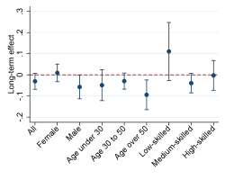
(a) Unemployment rate

Training

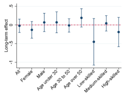
(b) Unsubsidised employment rate

Short measures

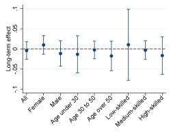
(c) Unemployment rate

Short measures

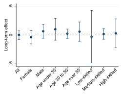
(d) Unsubsidised employment rate

Wage subsidies

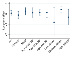
(e) Unemployment rate

Wage subsidies

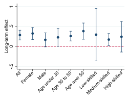
(f) Unsubsidised employment rate

Notes: This graphs show the long-term effects and the corresponding 96% CI of the three types of ALMP, i.e. training, short measures and wage subsidies on the unemployment and unsubsidised employment rates. The effects are based on the ARDL model estimated by 2SLS. Program variables are included with 6 lags, main sample restrictions apply. Standard errors obtained by a cross-sectional bootstrap (499 replications).

Figure 9: Longterm Effects for Different Subpopulations II

Training

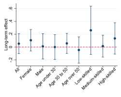
(a) Rate of welfare recipients

Training

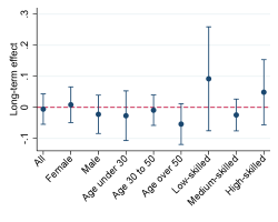
(b) Rate of employed workers on benefits

Short measures

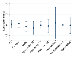
(c) Rate of welfare recipients

Short measures

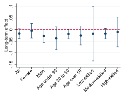
(d) Rate of employed workers on benefits

Wage subsidies

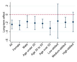
(e) Rate of welfare recipients

Wage subsidies

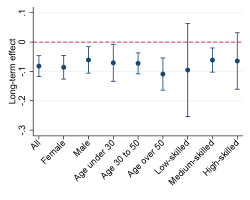
(f) Rate of employed workers on benefits

Notes: This graphs show the long-term effects and the corresponding 96% CI of the three types of ALMP, i.e. training, short measures and wage subsidies on the rate of welfare recipients and employed workers on benefits. The effects are based on the ARDL model estimated by 2SLS. Program variables are included with 6 lags, main sample restrictions apply. Standard errors obtained by a cross-sectional bootstrap (499 replications).

6 Robustness

6.1 Sensitivity to the Model Specification

We run two types of robustness checks to test for the sensitivity of the results to the model specification. First, we vary the lag order in the ARDL model and second, we estimate a distributed lag model, leaving out the lagged dependent variable.

The lag order.  Additionally to our main specification which includes all policy variables with 6 lags (corresponding to 6 quarters), we estimate two alternative specifications with 4 and 8 lags respectively. The optimal lag length is difficult to know ex-ante and usually a data-based choice. Choosing a lag length that is too short might potentially lead to biased estimates, a lag length that is too long merely decreases precision. Commonly used tests based on the Akaike information criterion (AIC) and the Schwartz/Bayesian information criterion (SBIC) (see e.g. Greene, 2012) are inconclusive in our setting. We therefore rely on a different approach and compare models based on a different lag order. The results are depicted in Appendix Figures A.14 and A.15 for our main outcomes. The figures depict the cumulative marginal effects for different lag orders and the 95% confidence interval for the main specification. All models yield qualitatively comparable results, with only small deviation in effect sizes. For all outcomes and policy variables, the cumulative effects curves lie within the confidence interval of the main specification. The effects of training slightly deviate from the main specification in the long run. Overall, the results suggest that the lag order does not play a major role in driving the effects.

Distributed lag model.  Next, we estimate an alternative model specification to test whether our results are sensitive to the inclusion of a lagged dependent variable in the model. For this, we estimate the same model as in equation (1) but leave out the yearly change in the lagged outcome. The distributed lag model still allows for a dynamic effect of the policy variables on the outcome but does not assume that the policies affect have an effect through intermediate outcomes. Similar to the ARDL model, the coefficient $\phi_{0}^{m}$ measures the short run effects of a policy. The long-run effect is given by the sum of lag weights $\sum_{j=0}^{q}\phi_{j}^{m}$. Both effects estimated by 2SLS are presented in Appendix Table LABEL:tab:dl_alo_emp. We find similar results as for the ARDL model with only small deviations in effect sizes. There is no evidence for an effect of short measures on labour market outcomes, the long-term effect of training on the unemployment rate is smaller in absolute value and insignificant. Also this model shows that wage subsidies significantly increase the unsubsidised employment rate in the long run, with the effect being slightly smaller. The effect is mostly driven by a reduction in the rate of welfare recipients. In sum, the results suggest that the policy effect that goes through intermediate outcomes is small. In turn, it is unlikely that our main effects suffer from a large bias introduced by the correlation of the error term with the lagged dependent variable. If anything, they represent a lower bound of the true effect.

6.2 Sensitivity to the Labour market Definition and Overlap Criteria

In a series of robustness checks, we test the sensitivity of our results to the choice of the labour market definition and overlap criteria.

Labour market definitions.  As introduced in Section 4.2 different stopping values in the clustering process lead to labour markets of different sizes and self-containment levels and also affect the overall number of markets in the estimation sample. Thus, we check whether our results change for different labour market definitions. Specifically, we compare the effects for labour market definitions depending on the stopping values 0.991, 0.993 and 0.997 with our main definition based on the stopping value 0.995. The results are displayed in Appendix Figure A.16 for the unemployment rate and the unsubsidised employment rate. Appendix Figure A.17 shows the results for the rate of welfare recipients and the rate of employed workers on benefits. The figures plot the cumulative marginal effects of different programs on the respective labour market outcome as separate lines for each labour market definition. The grey area depicts the 95% confidence interval for the main definition. We find very similar effect patterns for all labour market definitions and only small deviations in the long-term effects of training and wage subsidies. The effects of these programs are found to be slightly smaller for the definitions based on lower stopping values.

Overlap criteria.  In the following, we show that our results are robust to varying the strictness of overlap criteria which strongly supports our identification strategy. We test a number of different sample selection criteria based on the overlap between labour markets and employment agencies. For all checks, we impose that a labour market needs to overlap with at least two employment agencies and vary the restrictions on the size of the overlap on top. The overlap criteria are defined based on two shares. First, we consider the total overlap $s_{tot}$, which measures the RLF in the labour market as share of the total RLF in all partially overlapping agencies. Second, we consider the overlap between a market and single agencies, $s_{LEA}=RLF_{LLM,LEA}/RLF_{LEA}$. It measures the share of the agency’s labour force that overlaps between the market and the agency. The distribution of these two shares and our overlap criteria are shown in Appendix Figure A.18. Panel (a) plots the distribution of $s_{tot}$ for all labour markets in our preferred definition that overlap with at least two agencies. Panel (b) plots the distribution of $s_{LEA}$ for these markets and their overlapping agencies. Vertical lines depict how the sample is restricted by different criteria that we explain below.

We test three alternative criteria that target the validity of the exogeneity assumption. First, we impose a stricter exogeneity criterion and drop all labour markets for which $s_{tot}\geq$ 40% (exo1). Second, we relax this criterion and keep all labour markets for which $s_{tot}<$ 60% (exo2). As third restriction (exo3), we assess whether the overlap between the labour market and each agencies is not too large. If this is the case, our identification strategy is more credible, since policy mix in the agency is not fully determined by the economic situation in the market. Thus, we check for each labour market and agency whether the overlapping RLF comprises less than 50% of the RLF in the respective agency and only keep those labour markets in the sample for which the agencies which violate this restriction jointly represent less than 50% of the total labour force in the instrument area.

In order to assess the validity of the relevance assumption, we test four alternative criteria which we impose on top of the main sample restriction that limits $s_{tot}$ at 50%. First, we only consider labour markets that do not have fully enclosed agencies or in which enclosed agencies account for 50% or less of the RLF in the market (rel1). Second, we impose two minimum criteria on $s_{tot}$. The RLF in the labour market should constitute at least 5% (rel2) or 10% (rel3) of the overlapping agencies respectively. Finally, we review the overlap between a labour market and single agencies. Optimally, this overlap is large enough for all agencies that partially overlap with a market. Then the policy mix inside is most likely to correlate with the policy mix outside, e.g. through agency-specific strategies. Since imposing a minimum criterion on the overlap of each agency would be too restrictive, we propose the following two sample restrictions. First, the labour market must overlap sufficiently with at least one agency, such that $s_{LEA}>$ 20% (rel4). Second, the labour market must overlap sufficiently with at least two agencies, such that for these agencies $s_{LEA}>$ 10% (rel5).

Appendix Figure A.19 shows how our estimation sample changes after imposing these alternative sample selection criteria. With most of the criteria, we keep more than 90 labour markets. The reduction in the sample is largest for rel5. We plot the results of the ARDL model estimated in these different samples in Appendix Figures A.20 and A.21. They show the long-term effects of the different training programs separately for each of the main labour market outcomes. Overall, the point estimates are very robust to the variation in overlap criteria. Training and short measures do not have a robust effect on aggregate labour market outcomes, but we find a robust positive employment effect for wage subsidies that is explained by a reduction in the rate of welfare recipients or employed workers on benefits. The results strongly support the validity of our identification strategy and are not sensitive to stricter overlap criteria.

6.3 Sensitivity to the Reform in 2009

Finally, we test the sensitivity of our results to a change in the observation period. Motivated by the institutional changes of short measures in 2009, we estimate the effects of ALMP using a shorter time frame, i.e. 2010 to 2018. Appendix Table LABEL:tab:post2010_alo_emp shows the effects of the three policy types on our main set of outcomes estimated by 2SLS. As in our main analysis, we do not find any effect of short term measures on aggregate labour market outcomes. This suggests that absence of effects in our main analysis is not driven by the institutional framework. The long-term effect of training is negative but not statistically significant. Compared to the main analysis, we find a slightly smaller long-term effect of wage subsidies on the employment rate and a negative and significant effect on the unemployment rate. These changes might be partially driven by a different macroeconomic situation in the years 2005 to 2010, including the Great Recession in 2008.

7 Conclusion

Research on macroeconomic effects of ALMP confronts two important empirical challenges: First, policies and labour market outcomes are determined simultaneously on the aggregate level. Second, there might be spillover effects across neighbouring regions that are closely linked economically. This makes it difficult to identify policy effects on the aggregate level. This paper develops a new empirical strategy that allows us to address these challenges by studying effect of the level of self-contained local labour markets and by exploiting their imperfect overlap with the administrative regions that are in charge of policy decisions.

We apply this strategy to estimate the macroeconomic effects of ALMP in Germany over the period 2005 to 2018. We consider three types of policies: short activation measures, vocational training and wage subsidies and estimate their effects on aggregate labour market outcomes at the labour market level. We instrument the policy use in the labour market by the policy use in neighbouring municipalities that are part of the jurisdiction of local employment agencies that partially overlap with the labour market. We find no aggregate effects of a higher program use intensity of short activation measures and further vocational training on the aggregate employment rate. Wage subsidies in contrast, are effective in increasing employment and reducing long-term unemployment and welfare dependency. A 10 percentage point increase in the share of wage subsidy recipients increases the unsubsidised employment rate by 3 percentage points. Our findings further suggest that not all segments of the labour market are equally affected by the policies. Workers older than 50 years benefit more from a higher intensity of training programs and wage subsidies compared to younger workers. We also find differences in the effectiveness of programs across gender and skill groups, even though our estimates lack precision. Our results are robust to a variety of robustness checks such as changes in the model specification, different labour market definitions and overlap criteria.

Our findings bear important policy implications. A major part of the multi-billion euro investment in ALMP in recent decades did not result in a reduction of aggregate unemployment, which is the primary goal of these policies. Even if the policies are effective in increasing employment probabilities of program participants, our results suggest that these individual-level effects are partially offset by negative spillover effects on non-participants. The empirical strategy we apply in this paper does not allow us to directly quantify which workers and jobs are affected negatively. Nevertheless, our estimates inform about the net gain for all jobseekers in the labour market, which is a primary policy objective. Moreover, our suggestive evidence on heterogeneity in the effectiveness of policies for different labour market segments offers insights on potentially undesired redistribution of limited numbers of jobs across different labour market segments, and it might allow for a better targeting of policies to jobseekers. However, a better understanding of the link between individual-level effects and aggregate effects would be required in order to derive such policy recommendations.

Appendix A Appendix

A.1 Local Labour Markets

A.1.1 Municipalities and Municipality Regions

In this section we show how the three different aggregations of municipalities into municipality regions and their geographical distribution across Germany. Moreover, we assess whether the choice of the number of municipality regions in the range of 5000 to 7500 affects the self-containment of labour market definitions.

Figure A.1: Municipality Regions

(a) 5000

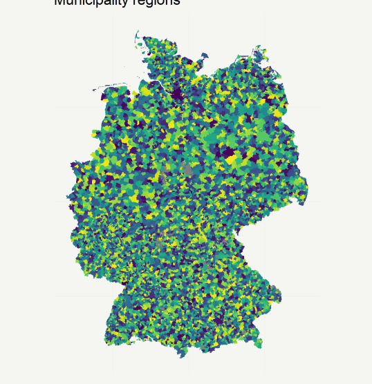
(b) 6000

(c) 7500

Notes: Municipality regions (5000, 6000, 7500) are depicted as coloured areas. Territorial status of 2016.

Table A.1: Characterizing Labour Market Definitions (Across Municipality Regions)

(1)	(2)	(3)	(4)	(5)	(6)	(7)	(8)	(9)	(10)
Def.	Municip. Reg.	Cut-off	N LLM	RLF (mean)	CR	ESC (mean)	ESC (sd)	ESC (min)	ESC(max)
1	6000	0.98	462	67652.63	20.22	65.77	16.46	11.11	98.27
2	6000	0.99	274	114071.22	15.91	74.03	13.07	11.11	98.27
3	6000	0.991	251	124523.96	14.89	75.50	12.24	11.11	98.27
4	6000	0.992	229	136486.96	14.08	76.63	11.75	11.11	98.27
5	6000	0.993	209	149547.91	13.57	78.03	10.44	16.56	98.27
6	6000	0.994	187	167141.79	12.78	79.11	10.43	16.56	98.27
7	6000	0.995	162	192935.27	12.06	80.71	8.34	45.88	98.27
8	6000	0.996	138	226489.23	11.10	82.35	7.78	54.43	98.27
9	6000	0.997	121	258310.03	10.35	83.41	7.61	54.43	98.27
10	6000	0.998	92	339733.85	8.21	86.39	5.44	65.34	98.27
11	6000	0.999	59	529754.47	5.83	89.68	3.81	76.56	98.27
12	5000	0.98	462	67652.63	21.01	65.32	16.39	10.39	98.27
13	5000	0.99	274	114071.22	16.51	74.27	11.61	16.70	98.27
14	5000	0.991	251	124523.96	16.03	75.40	11.17	16.70	98.27
15	5000	0.992	229	136486.96	14.90	76.46	10.31	39.95	98.27
16	5000	0.993	209	149547.91	14.35	77.47	9.86	44.82	98.27
17	5000	0.994	187	167141.79	13.15	79.01	9.10	44.82	98.27
18	5000	0.995	162	192935.27	12.16	80.08	9.38	44.82	98.27
19	5000	0.996	138	226489.23	11.45	82.11	7.86	48.88	98.27
20	5000	0.997	121	258310.03	10.55	83.48	7.25	48.88	98.27
21	5000	0.998	92	339733.85	8.92	86.07	5.69	67.81	98.27
22	5000	0.999	59	529754.47	6.72	89.07	4.71	72.93	98.27
23	7500	0.98	462	67652.63	18.84	64.34	19.20	5.24	98.27
24	7500	0.99	274	114071.22	14.83	73.80	14.08	8.73	98.27
25	7500	0.991	251	124523.96	14.02	75.35	12.77	11.11	98.27
26	7500	0.992	229	136486.96	13.39	76.52	12.31	11.11	98.27
27	7500	0.993	209	149547.91	12.91	77.61	11.66	11.11	98.27
28	7500	0.994	187	167141.79	12.06	79.13	10.44	11.11	98.27
29	7500	0.995	162	192935.27	11.09	80.94	8.90	41.93	98.27
30	7500	0.996	138	226489.23	10.20	82.40	8.47	53.74	98.27
31	7500	0.997	121	258310.03	9.40	83.92	7.65	56.41	98.27
32	7500	0.998	92	339733.85	7.87	85.87	6.89	60.42	98.27
33	7500	0.999	59	529754.47	5.65	89.03	5.44	64.71	98.27

Notes: The table compares different statistics for labour market definitions based on a different number of municipality regions (Column 2) and clustering cut-offs (Column 3). It displays the number of local labour markets (N LLM) in column 4, the average resident labour force (RLF (mean)) in column 5, the commuting ratio (CR) in column 6 and the mean, standard deviation and minimum and maximum employment self-containment ratio (ESC) in columns 7 to 10.

Table A.1 compares self-containment across labour market definitions for a different number of underlying municipality regions. It shows that the commuting ratio tends to be slightly lower for a higher number of underlying number of municipality regions. Nevertheless, the ESC ratio is not following a clear trend with regard to first level of aggregation. Overall, the choice of municipality regions in the first level of aggregation does not have a strong impact on the closedness of the labour markets.

A.1.2 Districts and Local Employment Agencies

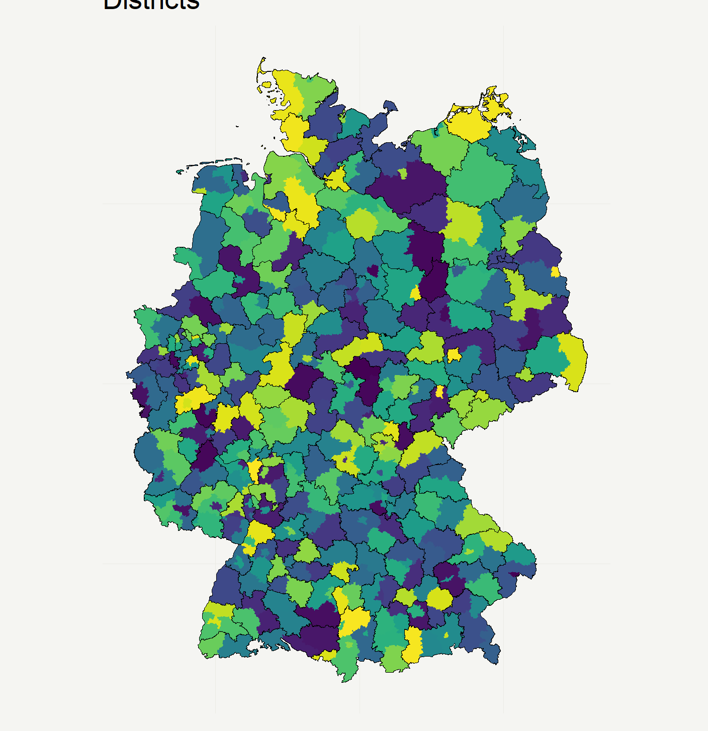
Figure A.2: Districts and Local Employment Agency Borders

Notes: 402 Districts are depicted as coloured areas, LEA borders are drawn in black. Territorial status of 2016.

A.1.3 Labour market definitions

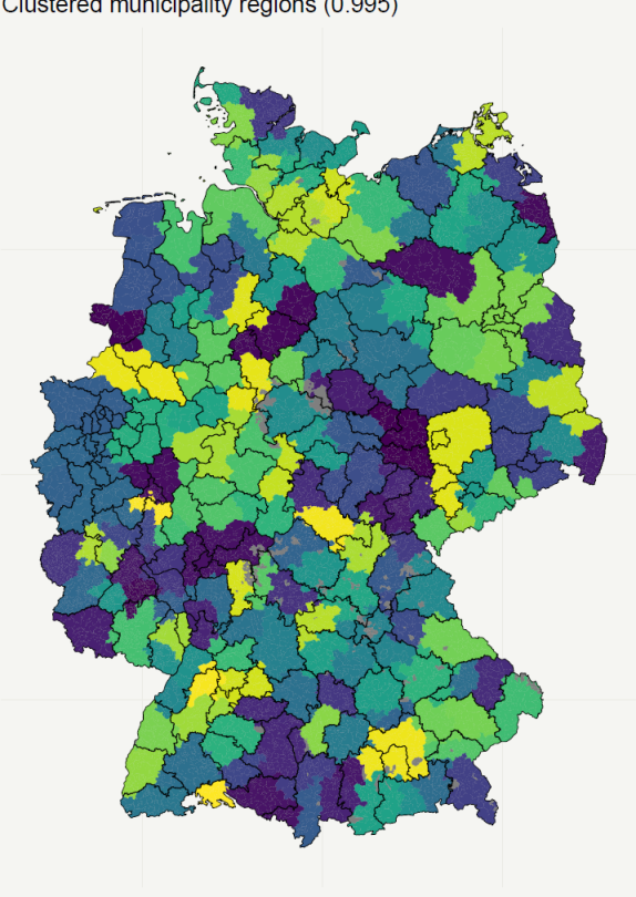
Figure A.3: Local Labour Markets and Local Employment Agency Borders

Notes: 162 Labour markets obtained by hierarchical clustering (average linkage) of 6000 municipality regions based on a dissimilarity matrix measuring the strength of commuting flows with an original cut-off value of 0.995. Labour markets are coloured areas, employment agency borders are drawn in black. Territorial status of 2016.

A.1.4 Consistency of Labour Market Definition over Time

While it has been documented that commuting distances in Germany increased over the last two decades (Dauth and Haller, 2018), it is not clear whether this increase will also lead to differences in the definition of labour markets. We thus check our main definition based on commuting flows in 2016 for consistency over time and additionally define labour markets based on the commuting flows in 2000 and 2009.

We calculate a similarity measure where for each municipality $m$, we count the number of municipalities which were assigned to the same labour market in year $t\in\{2002;2009\}$ and year $t^{\prime}\in\{2009;2016\}$ and divide it by the total number of municipalities in the market (except $m$) in year $t^{\prime}$. To account for the population density, we calculate a similar measure which weights the counts by the size of the local labour force in the respective municipalities.

Table A.2: Consistency of Labour Market Definitions over Time

	(1)	(2)	(3)	(4)	(5)	(6)
Year $t$-year $t^{\prime}$	All	All (weighted)	LLM centers	LLM centers (weighted)	N (year $t$)	N (year $t^{\prime}$)
2002-09	0.70	0.72	0.80	0.80	228	176
2002-16	0.64	0.67	0.74	0.73	228	161
2009-16	0.81	0.82	0.84	0.84	176	161

Table A.2 depicts averages of these shares for the comparison between the 2002 and 2016 and 2009 and 2016 for our preferred labour market definition. Column (1) and (2) report raw and population weighted averages of the shares by averaging over all municipalities. Column (3) and (4) average over the largest municipalities in the labour markets, i.e. the labour market centers. We find that after weighting by population density, around 70-80% of municipalities in a market remain the same across the three years that we consider. The shares are significantly higher when only inspecting labour market centers. We thus conclude that using our baseline definition of labour markets based on 2016 data should be sufficiently representative of the time period that we consider.

A.1.5 Comparability to Other Definitions of Local Labour Markets for Germany

Table A.3: Self-containment of Other Regional Delineations for Germany

	(1)	(2)	(3)	(4)	(5)	(6)
Delineation	N regions	CR	ESC (mean)	ESC (sd)	ESC (min)	ESC (max)
NUTS3 (districts)	402	38.1	58.9	13.6	20.5	86.7
LEA (local employment agencies)	156	27.3	71.5	10.8	45.6	91.6
SPR (spatial planning regions)	96	19.6	78.5	8.6	50.3	91.6
GRW (labour market regions of GRW)	258	25.5	69.3	10.3	32.7	91.2
RLM (regional labour markets)	141	19.9	75.9	9.4	42	91.3
LMR (labour market regions)	50	10.5	85.7	5	71.8	94.6
Our definition (6000, 995)	162	12.6	80.7	8.3	45.9	98.3

Notes: The table displays self-containment statistics for different regional delineations in Germany. It shows the number of regions (N regions) in column 1, the commuting ratio (CR) in column 2 and the mean, standard deviation and minimum and maximum employment self-containment ratio (ESC) in columns 3 to 6. Numbers for our definition are based on data from 2016, all others are based on 2014, calculated by Wicht et al. (2020).

Table A.3 shows the number of regions, the commuting share and two measures of self-containment for German districts, LEA, and four different definitions of local labour markets: 96 Spatial planning regions, 258 regions of the GRW (labour market regions of the Joint Task of the Federal Government and the federal states dedicated to the ‘Improvement of Regional Economic Structure’), 141 regions (RLM) defined by Kosfeld and Werner (2012) and 50 regions (LMR) defined by Kropp and Schwengler (2016). The numbers are based on calculations by Wicht et al. (2020) based on commuting flows for the year 2014. Two points are worth mentioning: First, it stands our that administrative regions such as LEA often used as units of analysis in comparable macro analyses for Germany are characterized by a comparatively lower levels of self-containment compared to most other labour market definitions. Second, our labour market definitions have comparable or even higher levels of self-containment and lower commuting shares for comparable numbers of labour markets.

A.2 Bias in the ARDL Model

In the following we show that the error term in an ARDL model estimated in yearly changes similar to equation (1) is correlated with the lagged dependent variable through its influences on past values of $y_{it}$. We abstract from covariates and policy variables for this exposition.

Given a model of the following form:

$\Delta y_{it}=\theta\Delta y_{i,t-1}+\Delta\varepsilon_{it}$

Backwards substitution leads to:

$\Delta y_{i,t-1}=\theta\Delta y_{i,t-2}+\Delta\varepsilon_{i,t-1}$

$\Delta y_{it}=\theta\left(\theta y_{i,t-2}+\Delta\varepsilon_{i,t-1}\right)+\Delta\varepsilon_{it}$

…

$\Delta y_{it}=\theta\left(\theta\left(\theta\left(\theta\left(\theta y_{i,t-5}+\Delta\varepsilon_{i,t-4}\right)+\Delta\varepsilon_{i,t-3}\right)+\Delta\varepsilon_{i,t-2}\right)+\Delta\varepsilon_{i,t-1}\right)+\Delta\varepsilon_{it}$

Since $\Delta\varepsilon_{i,t-4}=\varepsilon_{i,t-4}-\varepsilon_{i,t-8}$ and $\Delta\varepsilon_{it}=\varepsilon_{it}-\varepsilon_{i,t-4}$

$\Rightarrow C\left(\Delta y_{i,t-1},\Delta\varepsilon_{it}\right)\neq 0$.

A.3 Descriptive Statistics

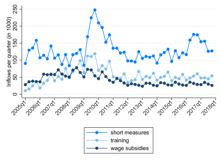
Figure A.4: Quarterly Inflows into Programs

Note: This graph plots the total inflows into the three different program types at the country level. Note that due to censoring of small values at the municipality level, these numbers are slightly under-reporting the true size of inflows.

Figure A.5: Regional Variation

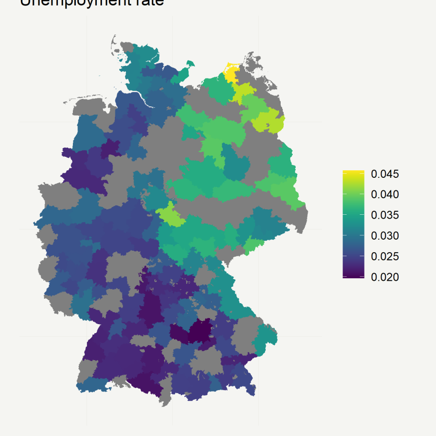
(a) Unemployment rate

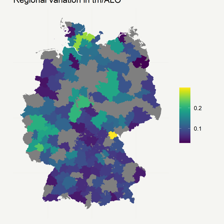
(b) Short measures

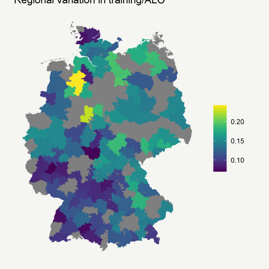
(c) Training

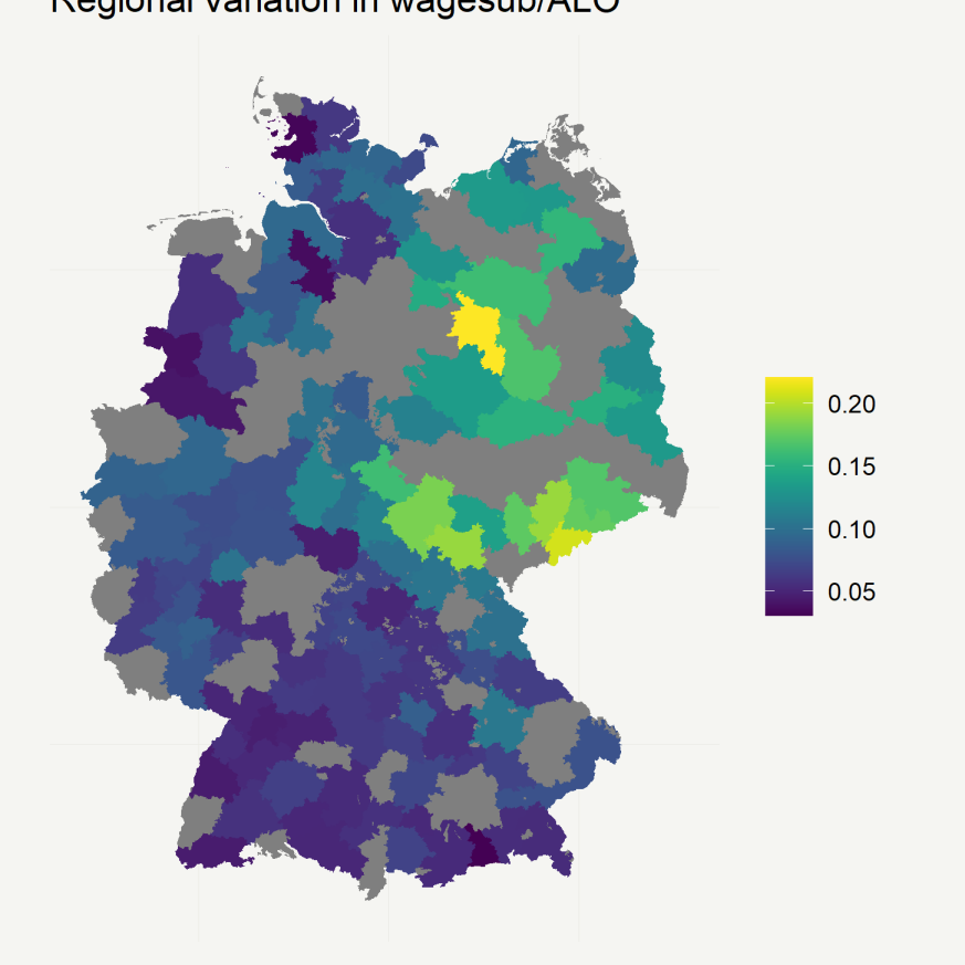
(d) Wage subsidies

Note: These graphs plot the average (a) unemployment rate, (b) accommodation rate in short measures, (c) training and (d) wage subsidies across the main estimation sample of labour markets by averaging over the years 2005 to 2018. Grey areas are not included in the sample.

Table A.4: Summary Statistics - Control Variables

	(1)	(2)	(3)	(4)
	mean	sd	min	max
Characteristics of the employed
Share German	0.92	0.14	0.00	1.00
Share female	0.49	0.02	0.44	0.58
Share 20-29 years*	0.19	0.02	0.10	0.25
Share 30-39 years	0.22	0.03	0.15	0.31
Share 40-49 years	0.30	0.03	0.20	0.40
Share 50-64 years	0.29	0.05	0.19	0.47
Share w/o schooling or high school degree*	0.85	0.05	0.67	0.95
Share w/ high school degree	0.15	0.05	0.05	0.33
Share w/o vocational training*	0.09	0.04	0.01	0.23
Share w/ vocational training	0.83	0.05	0.69	0.94
Share w/ academic degree	0.08	0.03	0.02	0.20
Share in primary sector and manufacturing	0.26	0.07	0.12	0.45
Share in construction, retail trade and transportation	0.31	0.03	0.22	0.45
Share in services and communication	0.12	0.03	0.05	0.22
Share in education, government work, culture and media*	0.31	0.04	0.20	0.44
Characteristics of the unemployed
Share female	0.44	0.05	0.22	0.65
Share 20-29 years*	0.23	0.04	0.06	0.39
Share 30-39 years	0.19	0.03	0.00	0.31
Share 40-49 years	0.21	0.03	0.05	0.35
Share 50-64 years	0.38	0.06	0.17	0.60
Share w/o schooling or high school degree*	0.85	0.06	0.00	0.97
Share w/ high school degree	0.15	0.06	0.00	0.38
Share w/o vocational training*	0.20	0.10	0.00	0.42
Share w/ vocational training	0.73	0.09	0.52	0.95
Share w/ academic degree	0.07	0.04	0.00	0.23
Share vocational degree censored	0.00	0.00	0.00	0.04
Share in primary sector and manufacturing	0.23	0.06	0.00	0.52
Share in construction, retail trade and transportation	0.39	0.06	0.17	0.70
Share in services and communication	0.15	0.04	0.00	0.31
Share in education, government work, culture and media	0.23	0.05	0.00	0.43
Other control variables
Share in programs for long-term unemployed (% of unemployed)	0.24	0.25	0.00	2.02
Share in programs for the young (% of unemployed)	0.05	0.03	0.00	0.24
Share in other programs (% of unemployed)	0.14	0.11	0.01	0.86
Resident Labour Force (in 10,000)**	18.55	22.77	1.60	137.98
Observations	5980
LLM	115

Notes: The table displays summary statistics for the control variables characterizing the employed and unemployed workforce for the period 2005 to 2018. Missing values were counted to the largest category. Censored values were flagged separately. * Reference categories. ** not used as control variable.

Table A.5: Summary Statistics - Policy and Outcome Variables

	(1)	(2)	(3)	(4)
	mean	sd	min	max
Program shares (labour markets)
Further vocational training	0.13	0.06	0.01	0.51
Short training	0.11	0.09	0.00	0.76
Wage subsidies	0.09	0.06	0.01	0.51
Program shares (instrument areas)
Further vocational training	0.13	0.05	0.02	0.35
Short training	0.11	0.07	0.01	0.50
Wage subsidies	0.09	0.06	0.01	0.40
Outcomes
Unemployment rate (% of LF)	0.03	0.01	0.01	0.12
Employment rate (% of LF)	0.86	0.07	0.57	0.97
Rate of welfare recipients (% of LF)	0.08	0.04	0.00	0.27
Rate of employed on benefits(% of LF)	0.03	0.02	0.01	0.09
Inflow rate into employment (% of LF)	0.02	0.00	0.01	0.05
Unemployment rate female	0.03	0.01	0.01	0.10
Unemployment rate male	0.03	0.01	0.01	0.13
Unemployment rate age under 30	0.03	0.02	0.01	0.14
Unemployment rate age 30 to 50	0.03	0.01	0.01	0.12
Unemployment rate age over 50	0.04	0.02	0.01	0.13
Unemployment rate low-educated	0.03	0.01	0.00	0.12
Unemployment rate highly-educated	0.03	0.01	0.00	0.11
Unemployment rate low-skilled	0.05	0.02	0.00	0.17
Unemployment rate medium skilled	0.03	0.01	0.01	0.12
Unemployment rate high-skilled	0.02	0.01	0.00	0.09
Employment rate female	0.87	0.06	0.61	0.97
Employment rate male	0.85	0.08	0.49	0.97
Employment rate age under 30	0.83	0.09	0.46	0.97
Employment rate age 30 to 50	0.86	0.07	0.57	0.97
Employment rate age over 50	0.83	0.08	0.47	0.96
Employment rate low educated	0.86	0.07	0.57	1.00
Employment rate high educated	0.86	0.07	0.49	1.00
Employment rate low-skilled	0.74	0.12	0.25	1.00
Employment rate medium skilled	0.87	0.07	0.56	0.98
Employment rate high-skilled	0.88	0.07	0.52	1.00
Observations	5980
LLM	115

Notes: The table displays summary statistics for the policy and outcome variables for the period 2005 to 2018.

A.4 Further Results

Table A.6: First Stage - Unsubsidized Employment Rate

	SW F-stat	SW p-val	AP F-stat	AP p-val
AR training	115.97	0.000	135.14	0.000
AR training (lag 1)	86.54	0.000	132.59	0.000
AR training (lag 2)	110.65	0.000	101.31	0.000
AR training (lag 3)	84.05	0.000	70.68	0.000
AR training (lag 4)	81.79	0.000	93.56	0.000
AR training (lag 5)	72.87	0.000	93.35	0.000
AR training (lag 6)	115.27	0.000	278.97	0.000
AR short measures	61.01	0.000	373.57	0.000
AR short measures (lag 1)	61.58	0.000	125.57	0.000
AR short measures (lag 2)	85.02	0.000	174.44	0.000
AR short measures (lag 3)	48.39	0.000	142.64	0.000
AR short measures (lag 4)	61.83	0.000	143.11	0.000
AR short measures (lag 5)	59.79	0.000	149.17	0.000
AR short measures (lag 6)	65.64	0.000	230.23	0.000
AR wage subsidies	103.32	0.000	435.60	0.000
AR wage subsidies (lag 1)	93.88	0.000	398.92	0.000
AR wage subsidies (lag 2)	99.85	0.000	202.76	0.000
AR wage subsidies (lag 3)	104.09	0.000	243.71	0.000
AR wage subsidies (lag 4)	105.92	0.000	212.58	0.000
AR wage subsidies (lag 5)	82.87	0.000	205.46	0.000
AR wage subsidies (lag 6)	119.28	0.000	489.47	0.000

Notes: The table reports three types of diagnostic test of the first stage for the 21 excluded instruments for the model including the lagged unsubsidized employment rate. Each line refers to a separate first-stage regression for the respective accommodation rate (AR). The first two columns show the conventional F-statistic of a joint test whether all instruments are significantly different from zero and the corresponding p-value. Columns 3 and 4 show the Sanderson-Windmeijer (2016) F statistics (SW F-stat) and p-values. Columns 5 and 6 the Angrist-Pischke (2009) F-statistics and p-values (AP F-stat).

Table A.7: First Stage - Rate of Welfare Recipients

	SW F-stat	SW p-val	AP F-stat	AP p-val
AR training	114.63	0.000	136.00	0.000
AR training (lag 1)	86.88	0.000	130.84	0.000
AR training (lag 2)	104.21	0.000	102.30	0.000
AR training (lag 3)	83.41	0.000	70.29	0.000
AR training (lag 4)	81.27	0.000	93.45	0.000
AR training (lag 5)	73.94	0.000	93.18	0.000
AR training (lag 6)	114.37	0.000	276.01	0.000
AR short measures	61.27	0.000	374.94	0.000
AR short measures (lag 1)	61.63	0.000	124.84	0.000
AR short measures (lag 2)	85.32	0.000	174.57	0.000
AR short measures (lag 3)	48.28	0.000	142.87	0.000
AR short measures (lag 4)	61.99	0.000	143.35	0.000
AR short measures (lag 5)	59.24	0.000	148.33	0.000
AR short measures (lag 6)	65.65	0.000	230.49	0.000
AR wage subsidies	102.93	0.000	433.97	0.000
AR wage subsidies (lag 1)	90.00	0.000	391.05	0.000
AR wage subsidies (lag 2)	100.40	0.000	203.33	0.000
AR wage subsidies (lag 3)	103.86	0.000	245.09	0.000
AR wage subsidies (lag 4)	106.09	0.000	212.67	0.000
AR wage subsidies (lag 5)	83.11	0.000	209.75	0.000
AR wage subsidies (lag 6)	118.79	0.000	489.82	0.000

Notes: The table reports three types of diagnostic test of the first stage for the 21 excluded instruments for the model including the lagged rate of welfare recipients. Each line refers to a separate first-stage regression for the respective accommodation rate (AR). The first two columns show the conventional F-statistic of a joint test whether all instruments are significantly different from zero and the corresponding p-value. Columns 3 and 4 show the Sanderson-Windmeijer (2016) F statistics (SW F-stat) and p-values. Columns 5 and 6 the Angrist-Pischke (2009) F-statistics and p-values (AP F-stat).

Table A.8: First Stage - Rate of Employed Workers on Benefits

	SW F-stat	SW p-val	AP F-stat	AP p-val
AR training	112.85	0.000	135.23	0.000
AR training (lag 1)	85.65	0.000	131.05	0.000
AR training (lag 2)	104.88	0.000	101.51	0.000
AR training (lag 3)	80.83	0.000	69.02	0.000
AR training (lag 4)	83.72	0.000	93.24	0.000
AR training (lag 5)	74.13	0.000	95.76	0.000
AR training (lag 6)	113.77	0.000	279.21	0.000
AR short measures	62.30	0.000	367.49	0.000
AR short measures (lag 1)	62.63	0.000	126.95	0.000
AR short measures (lag 2)	86.57	0.000	176.02	0.000
AR short measures (lag 3)	48.54	0.000	143.43	0.000
AR short measures (lag 4)	62.22	0.000	143.37	0.000
AR short measures (lag 5)	60.21	0.000	150.02	0.000
AR short measures (lag 6)	65.98	0.000	229.79	0.000
AR wage subsidies	103.35	0.000	437.69	0.000
AR wage subsidies (lag 1)	89.69	0.000	387.55	0.000
AR wage subsidies (lag 2)	99.87	0.000	214.19	0.000
AR wage subsidies (lag 3)	101.56	0.000	236.65	0.000
AR wage subsidies (lag 4)	110.38	0.000	215.68	0.000
AR wage subsidies (lag 5)	79.02	0.000	198.36	0.000
AR wage subsidies (lag 6)	119.59	0.000	515.27	0.000

Notes: The table reports three types of diagnostic test of the first stage for the 21 excluded instruments for the model including the lagged rate of employed workers on benefits. Each line refers to a separate first-stage regression for the respective accommodation rate (AR). The first two columns show the conventional F-statistic of a joint test whether all instruments are significantly different from zero and the corresponding p-value. Columns 3 and 4 show the Sanderson-Windmeijer (2016) F statistics (SW F-stat) and p-values. Columns 5 and 6 the Angrist-Pischke (2009) F-statistics and p-values (AP F-stat).

Figure A.6: Cumulative Marginal Effects for Females

Training

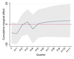
(a) Unemployment rate

Training

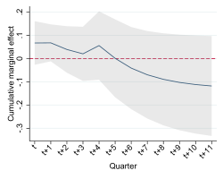
(b) Employment rate

Short measures

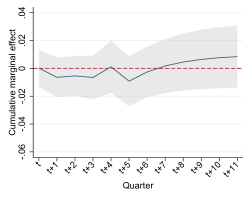
(c) Unemployment rate

Short measures

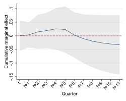
(d) Employment rate

Wage subsidies

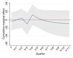
(e) Unemployment rate

Wage subsidies

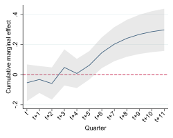
(f) Employment rate

Notes: These graphs show the cumulative marginal effects of the three types of ALMP, i.e. training, short measures and wage subsidies on the unemployment rate and unsubsidized employment rate. 95% confidence intervals are shown as grey areas. The effects are based on the ARDL model estimated by 2SLS. Program variables are included with 6 lags, main sample restrictions apply. Standard errors obtained by a cross-sectional bootstrap (499 replications).

Figure A.7: Cumulative Marginal Effects for Males

Training

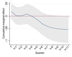
(a) Unemployment rate

Training

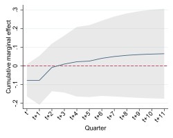
(b) Employment rate

Short measures

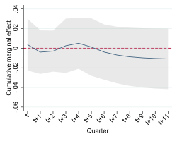
(c) Unemployment rate

Short measures

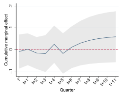
(d) Employment rate

Wage subsidies

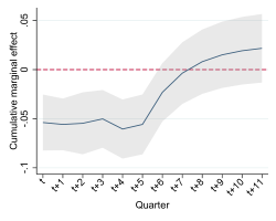
(e) Unemployment rate

Wage subsidies

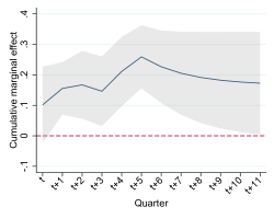
(f) Employment rate

Notes: These graphs show the cumulative marginal effects of the three types of ALMP, i.e. training, short measures and wage subsidies on the unemployment rate and unsubsidized employment rate. 95% confidence intervals are shown as grey areas. The effects are based on the ARDL model estimated by 2SLS. Program variables are included with 6 lags, main sample restrictions apply. Standard errors obtained by a cross-sectional bootstrap (499 replications).

Figure A.8: Cumulative Marginal Effects for Low-skilled

Training

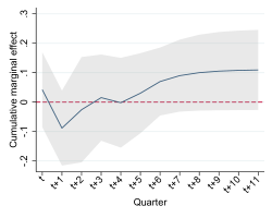
(a) Unemployment rate

Training

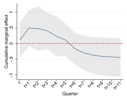
(b) Employment rate

Short measures

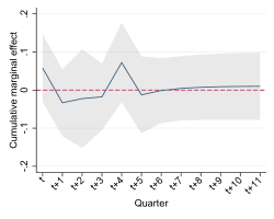
(c) Unemployment rate

Short measures

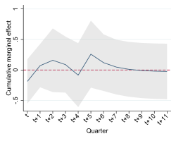
(d) Employment rate

Wage subsidies

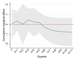
(e) Unemployment rate

Wage subsidies

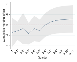
(f) Employment rate

Notes: These graphs show the cumulative marginal effects of the three types of ALMP, i.e. training, short measures and wage subsidies on the unemployment rate and unsubsidized employment rate. 95% confidence intervals are shown as grey areas. The effects are based on the ARDL model estimated by 2SLS. Program variables are included with 6 lags, main sample restrictions apply. Standard errors obtained by a cross-sectional bootstrap (499 replications).

Figure A.9: Cumulative Marginal Effects for Medium-skilled

Training

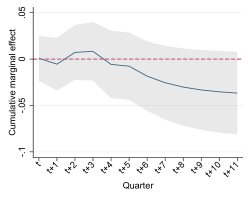
(a) Unemployment rate

Training

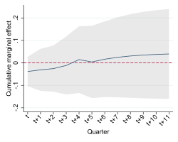
(b) Unsubsidized employment rate

Short measures

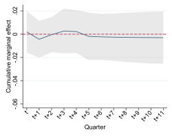
(c) Unemployment rate

Short measures

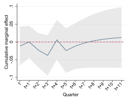
(d) Unsubsidized employment rate

Wage subsidies

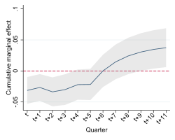
(e) Unemployment rate

Wage subsidies

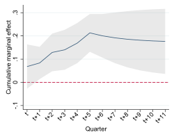
(f) Unsubsidized employment rate

Notes: These graphs show the cumulative marginal effects of the three types of ALMP, i.e. training, short measures and wage subsidies on the unemployment rate and unsubsidized employment rate. 95% confidence intervals are shown as grey areas. The effects are based on the ARDL model estimated by 2SLS. Program variables are included with 6 lags, main sample restrictions apply. Standard errors obtained by a cross-sectional bootstrap (499 replications).

Figure A.10: Cumulative Marginal Effects for High-skilled

Training

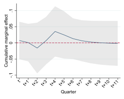
(a) Unemployment rate

Training

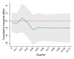
(b) Unsubsidized employment rate

Short measures

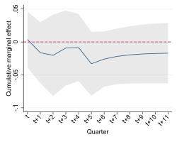
(c) Unemployment rate

Short measures

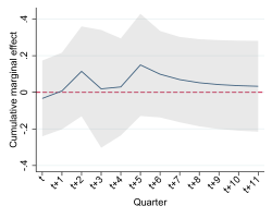
(d) Unsubsidized employment rate

Wage subsidies

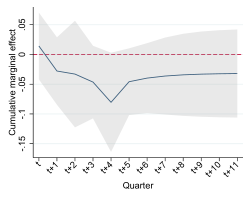
(e) Unemployment rate

Wage subsidies

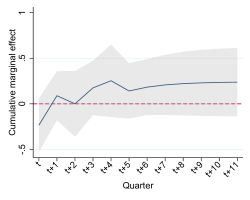
(f) Unsubsidized employment rate

Notes: These graphs show the cumulative marginal effects of the three types of ALMP, i.e. training, short measures and wage subsidies on the unemployment rate and unsubsidized employment rate. 95% confidence intervals are shown as grey areas. The effects are based on the ARDL model estimated by 2SLS. Program variables are included with 6 lags, main sample restrictions apply. Standard errors obtained by a cross-sectional bootstrap (499 replications).

Figure A.11: Cumulative Marginal Effects for Ages under 30

Training

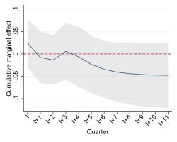
(a) Unemployment rate

Training

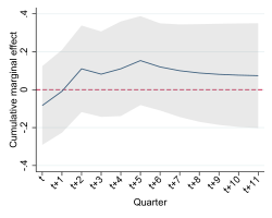
(b) Unsubsidized employment rate

Short measures

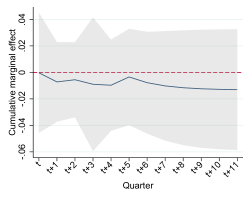
(c) Unemployment rate

Short measures

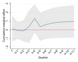
(d) Unsubsidized employment rate

Wage subsidies

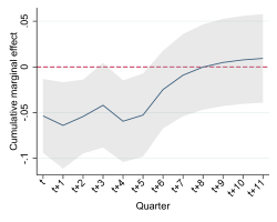
(e) Unemployment rate

Wage subsidies

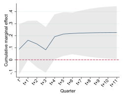
(f) Unsubsidized employment rate

Notes: These graphs show the cumulative marginal effects of the three types of ALMP, i.e. training, short measures and wage subsidies on the unemployment rate and unsubsidized employment rate. 95% confidence intervals are shown as grey areas. The effects are based on the ARDL model estimated by 2SLS. Program variables are included with 6 lags, main sample restrictions apply. Standard errors obtained by a cross-sectional bootstrap (499 replications).

Figure A.12: Cumulative Marginal Effects for Ages 30-50

Training

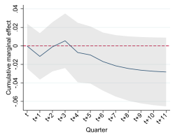
(a) Unemployment rate

Training

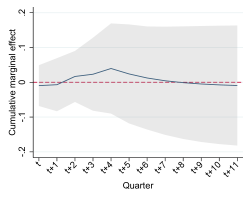
(b) Unsubsidized employment rate

Short measures

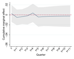
(c) Unemployment rate

Short measures

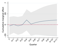
(d) Unsubsidized employment rate

Wage subsidies

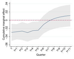
(e) Unemployment rate

Wage subsidies

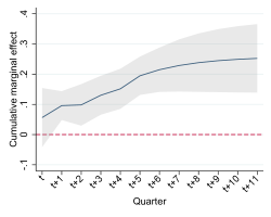
(f) Unsubsidized employment rate

Notes: These graphs show the cumulative marginal effects of the three types of ALMP, i.e. training, short measures and wage subsidies on the unemployment rate and unsubsidized employment rate. 95% confidence intervals are shown as grey areas. The effects are based on the ARDL model estimated by 2SLS. Program variables are included with 6 lags, main sample restrictions apply. Standard errors obtained by a cross-sectional bootstrap (499 replications).

Figure A.13: Cumulative Marginal Effects for Ages over 50

Training

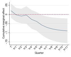
(a) Unemployment rate

Training

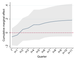
(b) Unsubsidized employment rate

Short measures

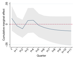
(c) Unemployment rate

Short measures

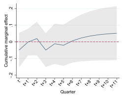
(d) Unsubsidized employment rate

Wage subsidies

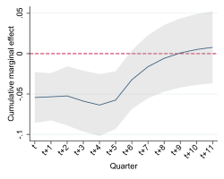
(e) Unemployment rate

Wage subsidies

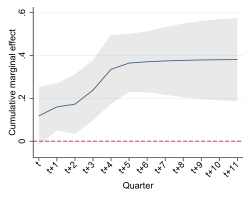
(f) Unsubsidized employment rate

Notes: These graphs show the cumulative marginal effects of the three types of ALMP, i.e. training, short measures and wage subsidies on the unemployment rate and unsubsidized employment rate. 95% confidence intervals are shown as grey areas. The effects are based on the ARDL model estimated by 2SLS. Program variables are included with 6 lags, main sample restrictions apply. Standard errors obtained by a cross-sectional bootstrap (499 replications).

Quarter-Year FEs $\checkmark$ $\checkmark$ $\checkmark$ $\checkmark$ Additional Controls $\checkmark$ $\checkmark$ $\checkmark$ $\checkmark$ Observations 5980 5980 5980 5980 LLM 115 115 115 115 Notes: This table shows the short-term (st) and long-term (lt) effects of the three types of ALMP, i.e. training, short measures (SM) and wage subsdies (wagesub) on the unemployment rate (columns 1-3), unsubsidized employment rate (columns 4-6), rate of welfare recipients (clumns 7-9) and rate of employed workers on benefits (columns 10-12). Program variables are included with 6 lags. The model is estimated for the time period 2010 to 2018. Standard errors (se) are obtained by a cross-sectional bootstrap (499 replications).

Figure A.14: Effect Patterns for Different Lag Order I

Training

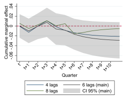
(a) Unemployment rate

Training

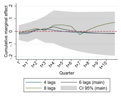
(b) Unsubsidised employment rate

Short measures

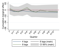
(c) Unemployment rate

Short measures

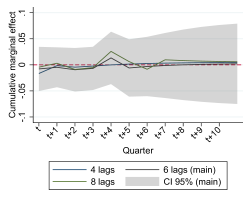
(d) Unsubsidised employment rate

Wage subsidies

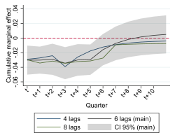
(e) Unemployment rate

Wage subsidies

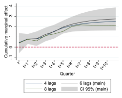
(f) Unsubsidised employment rate

Notes: These graphs show the cumulative marginal effects of the three types of ALMP, i.e. training, short measures and wage subsidies on the unemployment and unsubsidised employment rates. We show the effects for three models based on different lag orders. 95% confidence intervals for the model including policy variables with 6 lags are shown as grey areas. The effects are based on the ARDL model estimated by 2SLS. Main sample restrictions apply. Standard errors obtained by a cross-sectional bootstrap (499 replications).

Figure A.15: Effect Patterns for Different Lag order II

Training

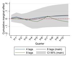
(a) Rate of welfare recipients

Training

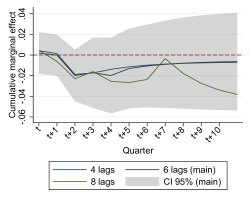
(b) Rate of employed workers on benefits

Short measures

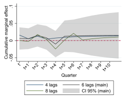
(c) Rate of welfare recipients

Short measures

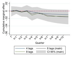
(d) Rate of employed workers on benefits

Wage subsidies

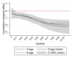
(e) Rate of welfare recipients

Wage subsidies

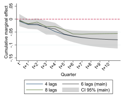
(f) Rate of employed workers on benefits

Notes: These graphs show the cumulative marginal effects of the three types of ALMP, i.e. training, short measures and wage subsidies on the rate of welfare recipients and employed workers on benefits. We show the effects for three models based on different lag orders. 95% confidence intervals for the model including policy variables with 6 lags are shown as grey areas. The effects are based on the ARDL model estimated by 2SLS. Main sample restrictions apply. Standard errors obtained by a cross-sectional bootstrap (499 replications).

Figure A.16: Effect Patterns for Different LLM Definitions I

Training

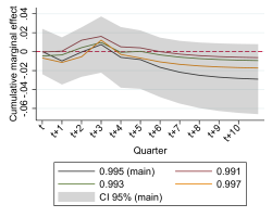
(a) Unemployment rate

Training

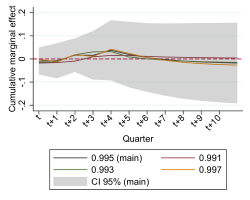
(b) Employment rate

Short measures

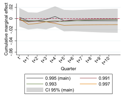
(c) Unemployment rate

Short measures

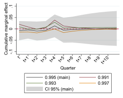
(d) Employment rate

Wage subsidies

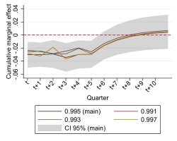
(e) Unemployment rate

Wage subsidies

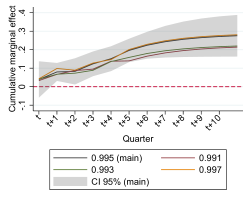
(f) Employment rate

Notes: These graphs show the cumulative marginal effects of the three types of ALMP, i.e. training, short measures and wage subsidies on the unemployment rate and unsubsidized employment rate. We show the effects for three models based on different labour market definitions. 95% confidence intervals for the main definition are shown as grey areas. The effects are based on the ARDL model estimated by 2SLS. Main sample restrictions apply. Standard errors obtained by a cross-sectional bootstrap (499 replications).

Figure A.17: Effect Patterns for Different LLM Definitions II

Training

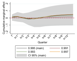
(a) Rate of welfare recipients

Training

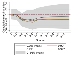
(b) Rate of employed workers on benefits

Short measures

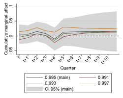
(c) Rate of welfare recipients

Short measures

(d) Rate of employed workers on benefits

Wage subsidies

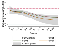
(e) Rate of welfare recipients

Wage subsidies

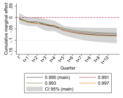
(f) Rate of employed workers on benefits

Notes: These graphs show the cumulative marginal effects of the three types of ALMP, i.e. training, short measures and wage subsidies on the rate of welfare recipients and employed workers on benefits. We show the effects for three models based on different labour market definitions. 95% confidence intervals for the main definition are shown as grey areas. The effects are based on the ARDL model estimated by 2SLS. Main sample restrictions apply. Standard errors obtained by a cross-sectional bootstrap (499 replications).

Figure A.18: Overlap Criteria

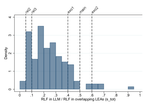
(a)

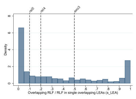
(b)

Notes: Panel (a) plots the distribution of the RLF in the labour market as share of the total RLF in all partially overlapping agencies across all labour markets that overlap with at least two agencies (131). Panel (b) plots the distribution of the overlapping RLF between each of these markets and agencies as share of the RLF in the agency for all market-agency combinations (468). Notice that the overlap measure in panel (b) is always strictly above zero. The minimum overlap is 0.0002.

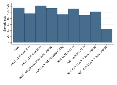
Figure A.19: Size of Subsamples (Relevance and Exogeneity Criteria)

Notes: The figure plots the sample size (number of labour markets) after imposing different overlap criteria targeting relevance and exogeneity.

Figure A.20: Long-term Effects for Different Subsamples (Relevance and Exogeneity Criteria)

Training

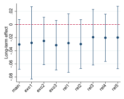
(a) Unemployment rate

Training

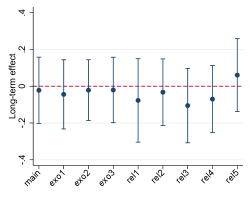
(b) Unsubsidzied employment rate

Short measures

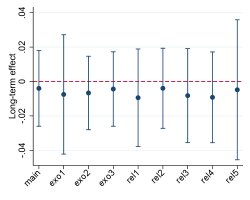
(c) Unemployment rate

Short measures

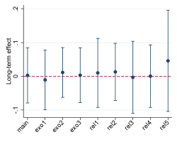
(d) Unsubsidzied employment rate

Wage subsidies

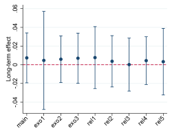
(e) Unemployment rate

Wage subsidies

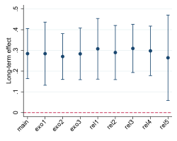
(f) Unsubsidzied employment rate

Notes: This graphs show the long-term effects and the corresponding 96% CI of the three types of ALMP, i.e. training, short measures and wage subsidies on the unemployment rate and unsubsidized employment rate. The effects on the x-axis are obtained by separate regressions based on different sample restrictions. The effects are based on the ARDL model estimated by 2SLS. Program variables are included with 6 lags. Standard errors obtained by a cross-sectional bootstrap (499 replications).

Figure A.21: Long-term Effects for Different Subsamples (Relevance and Exogeneity Criteria) II

Training

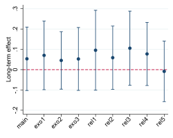
(a) Rate of welfare recipients

Training

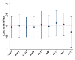
(b) Rate of employed workers on benefits

Short measures

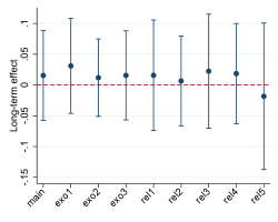
(c) Rate of welfare recipients

Short measures

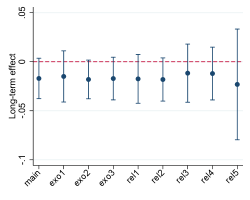
(d) Rate of employed workers on benefits

Wage subsidies

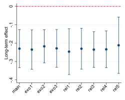
(e) Rate of welfare recipients

Wage subsidies

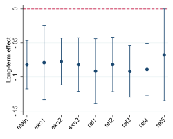
(f) Rate of employed workers on benefits

Notes: This graphs show the long-term effects and the corresponding 96% CI of the three types of ALMP, i.e. training, short measures and wage subsidies on the unemployment rate and unsubsidized employment rate. The effects on the x-axis are obtained by separate regressions based on different sample restrictions. The effects are based on the ARDL model estimated by 2SLS. Program variables are included with 6 lags. Standard errors obtained by a cross-sectional bootstrap (499 replications).

Quarter-Year FEs $\checkmark$ $\checkmark$ $\checkmark$ $\checkmark$ Additional Controls $\checkmark$ $\checkmark$ $\checkmark$ $\checkmark$ Observations 3680 3680 3680 3680 LLM 115 115 115 115 Notes: This table shows the effect on the lagged dependent variable, the short-term (st) and long-term (lt) effects of the three types of ALMP, i.e. training, short measures (SM) and wage subsdies (wagesub) on the unemployment rate (columns 1-3), unsubsidized employment rate (columns 4-6), rate of welfare recipients (clumns 7-9) and rate of employed workers on benefits (columns 10-12). The model is estimated for the time period 2010 to 2018. Standard errors (se) are obtained by a cross-sectional bootstrap (499 replications).

References

- (1)
- Abbring and Heckman (2007) Abbring, Jaap H. and James J. Heckman (2007). “Econometric Evaluation of Social Programs, Part III: Distributional Treatment Effects, Dynamic Treatment Effects, Dynamic Discrete Choice, and General Equilibrium Policy Evaluation”, in Handbook of Econometrics, 6B, Chap. 72: 5145–5303.
- Acemoglu and Autor (2011) Acemoglu, Daron and David Autor (2011). “Skills, Tasks and Technologies: Implications for Employment and Earnings”, in Handbook of Labor Economics, 4b, Elsevier B.V, Chap. 12: 1043–1171.
- Acemoglu and Restrepo (2020) Acemoglu, Daron and Pascual Restrepo (2020). “Robots and jobs: Evidence from us labor markets”, Journal of Political Economy, 128(6): 2188–2244.
- Altavilla and Caroleo (2013) Altavilla, Carlo and Floro E. Caroleo (2013). “Asymmetric Effects of National-based Active Labour Market Policies”, Regional Studies, 47(9): 1482–1506.
- Angrist and Pischke (2009) Angrist, J.D. and J.S. Pischke (2009). Mostly Harmless Econometrics : An Empiricist’s Companion, Princeton, Princeton University Press.
- Autor and Dorn (2013) Autor, David H. and David Dorn (2013). “The Growth of Low-Skill Service Jobs and the Polarization of the US Labor Market”, American Economic Review, 103(5): 1553–97.
- Autor et al. (2015) Autor, David H., David Dorn, and Gordon H. Hanson (2015). “Untangling Trade and Technology: Evidence from Local Labour Markets”, Economic Journal, 125(584): 621–646.
- Baker et al. (2005) Baker, Dean, Andrew Glyn, David Howell, and John Schmitt (2005). “Labor Market Institutions and Unemployment: A Critical Assessment of the Cross-Country Evidence”, in David R. Howell ed. Fighting unemployment: the limits of free market orthodoxy, Oxford University Press: 72–118.
- Bassanini and Duval (2007) Bassanini, Andrea and Romain Duval (2007). “The determinants of unemployment across OECD countries”, OECD Economic Studies, 2006(1): 7–86.
- Behaghel et al. (2014) Behaghel, Luc, Bruno Crépon, and Marc Gurgand (2014). “Private and Public Provision of Counseling to Job Seekers: Evidence from a Large Controlled Experiment”, American Economic Journal: Applied Economics, 6(4): 142–174.
- Bell et al. (1999) Bell, Brian, Richard Blundell, and John Van Reenen (1999). “Getting the Unemployed Back to Work: The Role of Targeted Wage Subsidies”, International Tax and Public Finance, 6(3): 339–360.
- Bergemann and Van den Berg (2008) Bergemann, Annette and Gerard J. Van den Berg (2008). “Active Labor Market Policy Effects for Women in Europe — A Survey”, Annales d’Économie et de Statistique, 91/92: 385–408.
- Biewen et al. (2014) Biewen, M., B. Fitzenberger, A. Osikominu, and M. Paul (2014). “The Effectiveness of Public-Sponsored Training Revisited: The Importance of Data and Methodological Choices”, Journal of Labor Economics, 32(4): 837–896.
- Bitler et al. (2006) Bitler, Marianne P., Jonah B. Gelbach, and Hilary W. Hoynes (2006). “What mean impacts miss: Distributional effects of welfare reform experiments”, American Economic Review, 96(4): 988–1012.
- Bjoerklund et al. (1991) Bjoerklund, Anders, Robert Haveman, Robinson Hollister, and Bertil Holmlund (1991). Labour market policy and unemployment insurance, Oxford, Clarendon Press.
- Blanchard and Wolfers (2000) Blanchard, Olivier and Justin Wolfers (2000). “The Role of Shocks and Institutions in the Rise of European Unemployment: The Aggregate Evidence”, The Economic Journal, 110(462): C1–C33.
- Blien (1998) Blien, Uwe (1998). “Die regionale Mittelverteilung für die aktive Arbeitsmarktpolitik”, Mitteilungen aus der Arbeitsmarkt- und Berufsforschung, 31(4): 674–689.
- Blien and Hirschenauer (2005) Blien, Uwe and Franziska Hirschenauer (2005). “Formula allocation: The regional allocation of budgetary funds for measures of active labour market policy in Germany”, IAB Discussion Paper, 11.
- Blundell et al. (2004) Blundell, Richard, Monica Costa Dias, Costas Meghir, and Can Reenen John (2004). “Evaluating the Employment Impact of a Mandatory Job Search Program on JSTOR”, Journal of the European Economic Association, 2(4): 569–606.
- Boeri and Burda (1996) Boeri, Tito and Michael C. Burda (1996). “Active labor market policies, job matching and the Czech miracle”, European Economic Review, 40(3-5): 805–817.
- Calmfors (1994) Calmfors, Lars (1994). “Active Labour Market Policy and Unemployment - A Framework for the Analysis of crucial Design Features”, OECD Economic Studies, 22(Spring): 7–47.
- Calmfors et al. (2002) Calmfors, Lars, Anders Forslund, and Maria Hemström (2002). “The effects of active labour market policies in Sweden : What is the evidence?”, in J. Agell, M.J. Keen, and A.J. Weichenreider eds. Labor Market Institutions and Public Regulation, Cambridge, MA, MIT Press, Chap. 1.
- Calmfors and Skedinger (1995) Calmfors, Lars and Per Skedinger (1995). “Does active labour-market policy increase employment? Theoretical considerations and some empirical evidence from Sweden”, Oxford Review of Economic Policy, 11(1): 91–109.
- Card et al. (2018) Card, David, Jochen Kluve, and Andrea Weber (2018). “What works? A meta analysis of recent active labor market program evaluations”, Journal of the European Economic Association, 16(3): 894–931.
- Caria et al. (2022) Caria, Stefano, Simon Franklin, and Marc Witte (2022). “Searching With Friends”, Journal of Labor Economics(forthcoming), DOI: http://dx.doi.org/10.1086/721655.
- Cockx et al. (2019) Cockx, Bart, Michael Lechner, and Joost Bollens (2019). “Priority to unemployed immigrants? A causal machine learning evaluation of training in Belgium”, CESifo WP, 8297.
- Crépon et al. (2013) Crépon, Bruno, Esther Duflo, Marc Gurgand, Roland Rathelot, and Philippe Zamora (2013). “Do labor market policies have displacement effects? Evidence from a clustered randomised experiment”, The Quarterly Journal of Economics, 128(2): 531–580.
- Dahlberg and Forslund (2005) Dahlberg, Matz and Anders Forslund (2005). “Direct Displacement Effects of Labour Market Programmes”, The Scandinavian Journal of Economics, 107(3): 475–494.
- Dauth and Haller (2018) Dauth, Wolfgang and Peter Haller (2018). “Berufliches Pendeln zwischen Wohn- und Arbeitsort: Klarer Trend zu längeren Pendeldistanzen”, IAB Kurzbericht, 10.
- Dauth et al. (2016) Dauth, Wolfgang, Reinhard Hujer, and Katja Wolf (2016). “Do Regions Benefit from Active Labour Market Policies? A Macroeconometric Evaluation Using Spatial Panel Methods”, Regional Studies, 50(4): 692–708.
- Doerr et al. (2017) Doerr, Annabelle, Bernd Fitzenberger, Thomas Kruppe, Marie Paul, and Anthony Strittmatter (2017). “Employment and earnings effects of awarding training vouchers in Germany”, Industrial and Labor Relations Review, 70(3): 767–812.
- Dustmann et al. (2009) Dustmann, Christian, Johannes Ludsteck, and Uta Schönberg (2009). “Revisiting the German Wage Structure”, The Quarterly Journal of Economics, 124(2): 843–881.
- Elmeskov et al. (1998) Elmeskov, Jorgen, John P Martin, and Stefano Scarpetta (1998). “Key lessons for labour market reforms: evidence from OEGD countries’ experiences”, Swedish Economic Policy Review, 5: 205–252.
- Escudero (2018) Escudero, Verónica (2018). “Are active labour market policies effective in activating and integrating low-skilled individuals? An international comparison”, IZA Journal of Labor Policy, 7(4): 1–26.
- Estevaõ (2003) Estevaõ, Marcello M. (2003). “Do Active Labor Market Policies Increase Employment?”, IMF Working Paper, 03(234).
- European Commission (2022) European Commission (2022). “LMP expenditure”, accessed(2022-07-13), available at https://webgate.ec.europa.eu/empl/redisstat/databrowser/product/page/LMP{_}IND{_}EXP.
- Ferracci et al. (2014) Ferracci, Marc, Grégory Jolivet, and Gerard J. van den Berg (2014). “Evidence of Treatment Spillovers Within Markets”, Review of Economics and Statistics, 96(5): 812–823.
- Fertig et al. (2006a) Fertig, Michael, Jochen Kluve, and Christoph M Schmidt (2006a). “Die makroökonomische Wirkung aktiver Arbeitsmarktpolitik - eine Panelanalyse auf Ebene regionaler Arbeitsmärkte”, Zeitschrift für Arbeitsmarktforschung, 3/4: 575–601.
- Fertig et al. (2006b) Fertig, Michael, Christoph M. Schmidt, and Hilmar Schneider (2006b). “Active labor market policy in Germany - Is there a successful policy strategy?”, Regional Science and Urban Economics, 36(3): 399–430.
- Fitzenberger et al. (2013) Fitzenberger, Bernd, Olga Orlanski, Aderonke Osikominu, and Marie Paul (2013). “Déjà Vu? Short-term training in Germany 1980–1992 and 2000–2003”, Empirical Economics, 44(1): 289–328.
- Fitzenberger et al. (2008) Fitzenberger, Bernd, Aderonke Osikominu, and Robert Völter (2008). “Get Training or Wait? Long-Run Employment Effects of Training Programs for the Unemployed in West Germany”, Annales d’Économie et de Statistique, 91/92: 321–355, DOI: http://dx.doi.org/10.2307/27917250.
- Galvao and Kato (2014) Galvao, Antonio F. and Kengo Kato (2014). “Estimation and Inference for Linear Panel Data Models Under Misspecification When Both n and T are Large”, Journal of Business & Economic Statistics, 32(2): 285–309.
- Gautier et al. (2018) Gautier, Pieter, Paul Muller, Bas van der Klaauw, Michael Rosholm, and Michael Svarer (2018). “Estimating Equilibrium Effects of Job Search Assistance”, Journal of Labor Economics, 36(4): 1073–1125.
- Gordo and Wolff (2011) Gordo, Laura Romeu and Joachim Wolff (2011). “Creating Employment or Keeping Them Busy? An Evaluation of Training Programs for Older Workers in Germany”, Journal of Aging & Social Policy, 23(2): 198–218.
- Greene (2012) Greene, W.H. (2012). Econometric Analysis, Pearson, 7th edition.
- Heckman et al. (1997) Heckman, James J., Jeffrey Smith, and Nancy Clements (1997). “Making The Most Out Of Programme Evaluations and Social Experiments: Accounting For Heterogeneity in Programme Impacts”, The Review of Economic Studies, 64(4): 487–535.
- Heuermann et al. (2015) Heuermann, Daniel F., Johannes F. Schmieder, and Philipp vom Berge (2015). “Evaluating Active Labor Market Policy in a Regression Discontinuity Design”, Unpublished Working Paper.
- Hirschenauer (2013) Hirschenauer, Franziska (2013). “Neue Typisierung der Agenturbezirke: Integrationserfolge hängen von regionalen Gegebenheiten ab”, IAB-Kurzbericht, 05/2013.
- Huber and Steinmayr (2021) Huber, Martin and Andreas Steinmayr (2021). “A Framework for Separating Individual-Level Treatment Effects From Spillover Effects”, Journal of Business and Economic Statistics, 39(2): 422–436.
- Hujer et al. (2009) Hujer, Reinhard, Paulo J. M. Rodrigues, and Katja Wolf (2009). “Estimating the Macroeconomic Effects of Active Labour Market Policies using Spatial Econometric Methods”, in U. Blien, E. Jahn, and G. Stephan eds. Unemployment and labour market policies - novel approaches (International Journal of Manpower. Special Issue), Bingley: 648–671.
- Hutter and Weber (2021) Hutter, Christian and Enzo Weber (2021). “Labour market miracle, productivity debacle: Measuring the effects of skill-biased and skill-neutral technical change”, Economic Modelling, 102 105584.
- Imbens and Wooldridge (2009) Imbens, Guido W. and Jeffrey M. Wooldridge (2009). “Recent Developments in the Econometrics of Program Evaluation”, Journal of Economic Literature, 47(1): 5–86.
- Jaenichen and Stephan (2011) Jaenichen, Ursula and Gesine Stephan (2011). “The effectiveness of targeted wage subsidies for hard-to-place workers”, Applied Economics, 43(10): 1209–1225.
- Johansson (2001) Johansson, Kerstin (2001). “Do labor market programs affect labor force participation?”, Swedish Economic Policy Review, 8: 215–234.
- Kapetanios (2008) Kapetanios, G. (2008). “A bootstrap procedure for panel data sets with many cross-sectional units”, The Econometrics Journal, 11(2): 377–395.
- Knaus et al. (2022) Knaus, Michael C, Michael Lechner, and Anthony Strittmatter (2022). “Heterogeneous Employment Effects of Job Search Programmes: A Machine Learning Approach”, Journal of Human Resources, 57(2): 597–636.
- Kopf (2013) Kopf, Eva (2013). “Short training for welfare recipients in Germany: Which types work?”, International Journal of Manpower, 34(5): 486–516.
- Kosfeld and Werner (2012) Kosfeld, Reinhold and Alexander Werner (2012). “Deutsche Arbeitsmarktregionen – Neuabgrenzung nach den Kreisgebietsreformen 2007–2011”, Raumforschung und Raumordnung, 70(1): 49–64.
- Kraft (1998) Kraft, Kornelius (1998). “An evaluation of active and passive labour market policy”, Applied Economics, 30(6): 783–793.
- Kropp and Schwengler (2008) Kropp, Per and Barbara Schwengler (2008). “Abgrenzung von Wirtschaftsräumen auf der Grundlage von Pendlerverflechtungen: Ein Methodenvergleich”, IAB-Discussion Paper(41).
- Kropp and Schwengler (2011a) (2011a). “Abgrenzung von Arbeitsmarktregionen – ein Methodenvorschlag”, Raumforschung und Raumordnung, 69(1): 45–62.
- Kropp and Schwengler (2011b) (2011b). “Empirische Regionalforschung heute”, in Christian Dreger, Reinhold Kosfeld, and Matthias Türck eds. Empirische Regionalforschung heute, Gabler Verlag: 195–211.
- Kropp and Schwengler (2012) (2012). “Vergleich von funktionalen Arbeitsmarktabgrenzungen in Deutschland”, Sozialer Fortschritt, 61(1): 11–20.
- Kropp and Schwengler (2016) (2016). “Three-Step Method for Delineating Functional Labour Market Regions”, Regional Studies, 50(3): 429–445.
- Kruppe (2009) Kruppe, Thomas (2009). “Bildungsgutscheine in der aktiven Arbeitsmarktpolitik”, Sozialer Fortschritt, 1: 9–19.
- Kruppe and Lang (2018) Kruppe, Thomas and Julia Lang (2018). “Labour market effects of retraining for the unemployed: the role of occupations”, Applied Economics, 50(14): 1578–1600.
- Laan and Schalke (2001) Laan, Lambert Van Der and Richard Schalke (2001). “Reality versus Policy: The Delineation and Testing of Local Labour Market and Spatial Policy Areas”, European Planning Studies, 9(2): 201–221.
- Lalive et al. (2015) Lalive, Rafael, Camille Landais, and Josef Zweimüller (2015). “Market externalities of large unemployment insurance extension programs”, American Economic Review, 105(12): 3564–3596.
- Layard et al. (1991) Layard, Richard, S. J. Nickell, and Richard Jackman (1991). Unemployment : macroeconomic performance and the labour market, Oxford, Oxford University Press.
- Layard et al. (2005) Layard, Richard, Stephen Nickell, and Richard Jackman (2005). Unemployment: Macroeconomic Performance and the Labour Market, Oxford University Press, 2nd edition.
- Lechner et al. (2011) Lechner, Michael, Ruth Miquel, and Conny Wunsch (2011). “Long-Run Effects of Public Sponsored Training in West Germany”, Journal of the European Economic Association, 9(4): 742–784.
- Lechner et al. (2015) Lechner, Michael, Patricyja Scioch, and Conny Wunsch (2015). “Do Firms Benefit from Active Labour Market Policies?”, Revised Version of IZA Discussion Paper, No. 7614.
- Matysik et al. (2014) Matysik, Alexander, Martin Leusch, and Günter Warsewa (2014). “Bildungszielplanung in der Arbeitsförderung: Struktur und Funktion im Land Bremen”, Reihe Arbeit und Wirtschaft in Bremen, 5.
- McCall et al. (2016) McCall, B., J. Smith, and C. Wunsch (2016). “Government-Sponsored Vocational Education for Adults”, Handbook of the Economics of Education, 5: 479–652.
- Mortensen and Pissarides (1994) Mortensen, Dale T. and Christopher A. Pissarides (1994). “Job creation and job destruction in the theory of unemployment”, Review of Economic Studies, 61(3): 397–415.
- Nickell (1981) Nickell, Stephen (1981). “Biases in Dynamic Models with Fixed Effects”, Econometrica, 49(6) 1417.
- Nickell (1997) (1997). “Unemployment and Labor Market Rigidities: Europe versus North”, The Journal of Economic Perspectives, 11(3): 55–74.
- Nickell (1998) (1998). “Unemployment: Questions and Some Answers”, The Economic Journal, 108(448): 802–816.
- Nickell and Layard (1999) Nickell, Stephen and Richard Layard (1999). “Labor market institutions and economic performance”, in Orley C. Ashenfelter and David Card eds. Handbook of Labor Economics, 3, Part C, Chap. Chapter 46: 3029–3084.
- Osikominu (2013) Osikominu, Aderonke (2013). “Quick Job Entry or Long-Term Human Capital Development? The Dynamic Effects of Alternative Training Schemes”, The Review of Economic Studies, 80(1): 313–342.
- Osikominu (2021) (2021). “The dynamics of training programs for the unemployed”, IZA World of Labor, 227(2): 1–12.
- Pissarides (2000) Pissarides, Christopher A. (2000). Unemployment equilibrium theory, MIT Press, 2nd edition.
- Puhani (2003) Puhani, Patrick A. (2003). “Active labour market policy and employment flows: Evidence from Polish regional data”, International Journal of Manpower, 24(8): 897–915.
- Sanderson and Windmeijer (2016) Sanderson, Eleanor and Frank Windmeijer (2016). “A weak instrument F-test in linear IV models with multiple endogenous variables”, Journal of Econometrics, 190(2): 212–221.
- Scarpetta (1996) Scarpetta, Stefano (1996). “Assessing the Role of Labour Market Policies and Institutitonal Settings on Unemployment: A Cross-Country Study”, OECD Economic Studies, 1(26): 43–98.
- Seele (2018) Seele, Stefanie (2018). “Essays on the German Labor Market since Unification”, Dissertation, Humboldt-Universität zu Berlin.
- Stephan (2010) Stephan, Gesine (2010). “Employer wage subsidies and wages in Germany: empirical evidence from individual data”, Zeitschrift fur Arbeitsmarktforschung, 43(1): 53–71.
- Stephan and Pahnke (2011) Stephan, Gesine and André Pahnke (2011). “The Relative Effectiveness of Selected Active Labor Market Programs: An Empirical Investigation for Germany”, The Manchester School, 79(6): 1262–1293.
- Tolbert and Killian (1987) Tolbert, Charles M. and Molly Sizer Killian (1987). “Labor Market Areas for the United States”,Technical report, Economic Research Service (DOA), Washington, D.C.
- Tolbert and Sizer (1996) Tolbert, Charles M. and Molly Sizer (1996). “U.S. Commuting Zones and Labor Market Areas - A 1990 Update”.
- Wapler et al. (2018) Wapler, Rüdiger, Daniel Werner, and Katja Wolf (2018). “Active labour market policies in Germany: do regional labour markets benefit?”, Applied Economics, 50(51): 5561–5578.
- Wapler et al. (2022) Wapler, Rüdiger, Katja Wolf, and Joachim Wolff (2022). “Do Active Labor Market Policies for Welfare Recipients in Germany Raise their Regional Outflow into Work?”, Journal of Policy Modeling.
- Wicht et al. (2020) Wicht, Alexandra, Per Kropp, and Barbara Schwengler (2020). “Are functional regions more homogeneous than administrative regions? A test using hierarchical linear models”, Papers in Regional Science, 99(1): 135–164.
- Wolff and Stephan (2013) Wolff, Joachim and Gesine Stephan (2013). “Subsidized work before and after the German Hartz reforms: design of major schemes, evaluation results and lessons learnt”, IZA Journal of Labor Policy, 2(1): 1–24.
- Wunsch (2005) Wunsch, Conny (2005). “Labour Market Policy in Germany: Institutions, Instruments and Reforms since Unification”, Discussion Paper University of St. Gallen, Department of Economics, No. 06.
- Wunsch (2013) (2013). “Optimal Use of Labor Market Policies: The Role of Job Search Assistance”, The Review of Economics and Statistics, 95(3): 1030–1045.
- Wunsch and Lechner (2008) Wunsch, Conny and Michael Lechner (2008). “What did all the money do? On the general ineffectiveness of recent west German labour market programmes”, Kyklos, 61(1): 134–174.
- Yankova (2010) Yankova, Katerina (2010). “Der Selektionsprozess in Maßnahmen der aktiven Arbeitsmarkt-politik”, IAB Discussion Paper, 11.