Non-conservation of the valley density and its implications for the observation of the valley Hall effect

Abstract

We show that the conservation of the valley density in multi-valley and time-reversal-invariant insulators is broken in an unexpected way by the electric field that drives the valley Hall effect. This implies that fully-gapped insulators can support a valley Hall current in the bulk and yet show no valley density accumulation on the edges. Thus, the valley Hall effect cannot be observed in such systems. If the system is not fully gapped then valley density accumulation at the edges is possible and can result in a net generation of valley density. The accumulation has no contribution from undergap states and can be expressed as a Fermi surface average, for which we derive an explicit formula. We demonstrate the theory by calculating the valley density accumulations in an archetypical valley-Hall insulator: a gapped graphene nanoribbon. Surprisingly, we discover that a net valley density polarization is dynamically generated for some types of edge terminations.

Introduction—The valley Hall effect (VHE) in non-topological systems has recently stirred considerable controversy [1, 2, 3, 4, 5, 6, 7, 8, 9, 9]. When the band structure features two valleys with a non-vanishing distribution of Berry curvature, electrons skew in the direction orthogonal to the applied electric field, even in the absence of magnetic field. However, since the system is not topological, electrons originating from one valley skew in the opposite direction of those from the other valley giving rise to a zero (charge) Hall current but to a finite valley Hall current ${\bm{j}}_{v}({\bm{r}},t)$. This is defined as the difference between charge currents of electrons originating in opposite valleys. When this current hits the edge of the system, a valley density $n_{v}({\bm{r}},t)$ (or, more physically, a density of orbital magnetic moment [10]), is expected to accumulate at its boundaries. This assumes that the valley density obeys a standard continuity equation [5, 6]. This seems a reasonable assumption: the two valleys are well-separated in momentum space, up to the point that they could ideally be taken as completely disconnected.

Some authors [1, 6] went further and claimed that even a fully-gapped non-topological insulator such as graphene aligned with hexagonal boron nitride (hBN) [3, 4] can exhibit nonlocal charge transport mediated by transverse undergap valley currents flowing in the bulk of the material. The authors of Ref. [6] argued that, at finite temperature, the valley-density accumulation could drive a “squeezed edge current” (parallel to the edges) in apparent agreement with experimental observations [2]. However, other authors [7, 8, 9] found from microscopic calculations that there is no valley density accumulation and no edge current in the simple graphene/hBN model. They proposed that the observed nonlocal resistances are caused by substrate-induced edge states crossing the Fermi level [7] or by substrate-induced valley-dependent scattering [9]. In the case of a fully gapped insulator this leaves us with the following puzzle: on one hand, the electric field drives a finite dissipationless valley Hall current in the bulk; on the other hand, time reversal symmetry implies that a valley density accumulation—a time-reversal-odd quantity—cannot appear in response to an electric field, unless there is dissipation, which is impossible if there are no states at the Fermi level. So where did the valley current go?

In this paper we solve the puzzle by observing that the valley density does not satisfy the conventional continuity equation when an electric field is present. This includes the field applied in order to drive the valley Hall current. The reason is that the electric field breaks the conservation of crystal momentum and therefore of valley number, which depends explicitly on crystal momentum. As a result, the bulk valley current is internally short-circuited as electrons flow from one valley to the other (and thus switch the sign of the Berry curvature) under the action of the very same electric field that drives the valley Hall current in the first instance. The process is schematically illustrated in Fig. 1.

Our results have profound implications for the observation of the VHE [11]. In a fully gapped time-reversal invariant insulator the undergap valley current is incapable of producing a valley density accumulation on the edge. This makes observing the VHE impossible in such systems, unless, e.g., the valley degeneracy is lifted (see, for example, Refs. [12, 13, 14]) or carriers are selectively injected into a single valley via circularly polarized light [15]. In these cases, however, an anomalous Hall effect “in disguise” is measured. This also means that the non-local resistance detection in Refs. [1, 16, 17, 18, 19] must have been caused by partially occupied bands or edge states.

In metallic systems, which support a Fermi surface, our predictions for the valley density accumulation are quite different from those of the conventional theory which treats the entire bulk valley Hall current as the source of the accumulation. In particular, the value of the accumulation depends on the form of the electronic wave functions near the edge. The length over which it occurs is not related to the carrier diffusion length as in, e.g., Ref. [5], but reflects the much shorter localization length of edge states, as observed in some experiments [20], or the Fermi wavelength of bulk states. Perhaps the most important result of this study is that the valley density in the VHE is not simply transported from one edge to the other: it can be simultaneously generated on both edges by processes that involve the electric field in the bulk of the material.

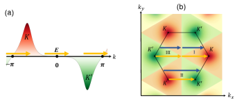
Figure 1: Cyclic flow of the Bloch wave vector under the action of an electric field in the $x$ direction. In both panels, the valley charge is $-1$ in the red regions and $+1$ in the green regions. Also shown are the Berry curvature hot spots with positive value near $K$ and negative value near $K^{\prime}$. Panel (a) shows the flow in a one-dimensional ribbon where the valley charge is non-conserved (changes sign) when $k$ crosses the origin of momentum space. At the same time the Berry curvature, and hence the anomalous velocity also changes sign ensuring the existence of a steady valley Hall current. In a fully gapped insulator the flow does not alter the occupation of the states (i.e., a full band remains full) so there is no change in the valley density. Panel (b) shows examples of flows in a two-dimensional periodic system. In both cases the assumption of time-reversal symmetry rules out the possibility of a valley density response arising from the magneto-electric polarizability of the Bloch states.

Summary of main ideas—We consider a generic system in the shape of a strip of finite width which is indefinitely extended along the $x$ axis. As we show below, the continuity equation satisfied by the valley density is

$$\partial_{t}n_{v}(y,t)+\partial_{y}j^{y}_{v}(y,t)=-e^{2}E(t)\sum_{k}S(k)\partial_{k}f_{k}(y)\,,$$ (1)

where the electric field is in the $x$ direction, which is parallel to the edge, and the valley current is in the $y$ direction, perpendicular to the edge . The system is assumed to be macroscopically homogeneous along $x$ so that the valley density and current depend only on $y$. The electronic states (in the absence of the electric field) are taken to be of the form $\psi_{k,n}(x,y)=e^{ikx}u_{k,n}(x,y)/\sqrt{2\pi}$ where $k$ is the $x$-component of the Bloch wave vector and $n$ is the band index. The sum over $k$ in Eq. (1) stands for $\int dk/(2\pi)$. The mixed electronic distribution $f_{k}(y)=a^{-1}\int_{0}^{a}dx\sum_{n}f_{k,n}\big{|}u_{k,n}(x,y)\big{|}^{2}$ is defined in terms of the electronic wave functions and the occupations of the corresponding states $f_{k,n}$, with the integral taken over one period $a$ in the $x$ direction. $S(k)$ is a “valley charge” function (odd under time reversal), which is a smooth periodic function of $k$ in the Brillouin zone. We assume that the band structure features only two valleys, thus $S(k)$ assigns number $+1$ to states around one valley and $-1$ to states around the other valley. The valley density operator is $\hat{n}_{v}(\bm{r})\equiv-(e/2)\sum_{j}\big{\{}S(\hat{k}_{j}),\delta(\bm{r}-\hat{\bm{r}}_{j})\big{\}}$ where $\hat{\bm{r}}_{j}$ and $\hat{k}_{j}$ are the position and Bloch momentum operator (along the edge) of the $j$-th electron, respectively, and $\{\hat{A},\hat{B}\}\equiv\big{(}\hat{A}\hat{B}+\hat{B}\hat{A}\big{)}$. The valley current density is $\bm{\hat{j}}_{v}(\bm{r})\equiv-(e/4)\sum_{j}\big{\{}S(\hat{k}_{j}),\big{\{}\hat{\bm{v}}_{j}\,,\delta(\bm{r}-\hat{\bm{r}}_{j})\big{\}}\big{\}}$, where $\hat{\bm{v}}_{j}$ is the velocity operator of the $j$-th electron. Because $\hat{k}$ is a constant of motion, $\hat{n}_{v}$ and $\bm{\hat{j}}_{v}(\bm{r})$ obey a conventional continuity equation in the absence of the electric field.

As we show below, in a fully gapped time-reversal invariant insulator, in which no edge or bulk state crosses the Fermi level, and at zero temperature, the right-hand side of Eq. (1) completely cancels the nearly-quantized contribution due to the second term on the left hand side. In this case, therefore, the valley density accumulation vanishes, even though there is a finite valley current in the bulk. In all other cases the cancellation is not exact. The correct equation for the density accumulation in the absence of relaxation processes is then $\partial_{t}n_{v}(y,t)=-Q_{s}(y)$, where the source term

$$Q_{s}(y)=\frac{e^{2}E}{a}\int_{0}^{a}dx\sum_{k,n}\left(\partial_{k}f_{k,n}\right)S(k)\big{|}u_{k,n}(x,y)\big{|}^{2}\,,$$ (2)

is a Fermi surface property. Note that $Q_{s}(y)$ cannot be written, in general, as the divergence of a current. In fact, this is only possible if its integral over the whole strip vanishes, which implies that density accumulates at one edge and depletes at the other . However, if the width of the strip is macroscopically large, the source term is localized on the edges. One can then define the “effective current” $I_{s}$, obtained by integrating Eq. (2) across a given edge, that feeds the valley number accumulation thereat. Since valley density is not conserved, the sum of the effective currents associated with the two edges does not have to be zero. $I_{s}$ can be split as $I_{s}=I_{s}^{e}+I_{s}^{b}$, where $I_{s}^{e}=e^{2}E\sum_{k,e}\left(\partial_{k}f_{k,e}\right)S(k)$ is the contribution of edge states. Here, the sum over $e$ is that over edge states. The calculation of the contribution of bulk states, $I_{s}^{b}$, is complicated by the fact that the integral over $y$ cannot be extended to infinity before performing the sum over $n$ and $k$: the result would diverge. Nevertheless, a closed expression can be obtained in terms of the probability amplitude for Bloch waves to scatter off the edge [see Eq. (6) below]. Once $I_{s}$ is known, the valley number accumulation can be estimated as $I_{s}\tau_{tr}$, where $\tau_{tr}$ is the intra- or inter-valley momentum relaxation time for the bulk or edge states’ contribution, respectively.

Anomalous continuity equation—We consider a 2D crystal periodic in the $x$ direction with period $a=1$ and with the edges positioned at $y=0$ and $y=-W$. A uniform electric field of magnitude $E$ oscillating at frequency $\omega$ is applied along the $x$ direction. For the sake of conciseness, hereafter we set $\hbar=1$. Thus the conductance quantum $e^{2}/h$ is equal to $e^{2}/(2\pi)$, where $e$ is the electron charge. From the Kubo formula [24, 25], the $y$ component of the valley current (averaged over $x$) is  

$$j_{v}^{y}(y,\omega) = iEe^{2}\sum_{k,n,n^{\prime}}\int_{0}^{y}dy^{\prime}(\varepsilon_{k,n}-\varepsilon_{k,n^{\prime}})$$ (3)

$$\times S(k){\cal L}_{k,nn^{\prime}}(\omega){\cal W}_{k,nn^{\prime}}(y^{\prime})\mathcal{A}_{k,n^{\prime}n},$$

and the valley density (also averaged over $x$)

$$n_{v}(y,\omega)=-\frac{iEe^{2}}{\omega+i0}\sum_{k,n}\partial_{k}f_{k,n}\,S(k)\,{\cal W}_{k,nn}(y)$$

$$-Ee^{2}\sum_{k,n,n^{\prime}}S(k){\cal L}_{k,nn^{\prime}}(\omega){\cal W}_{k,nn^{\prime}}(y)\mathcal{A}_{k,n^{\prime}n},$$ (4)

where ${\cal L}_{k,nn^{\prime}}(\omega)\equiv(f_{k,n}-f_{k,n^{\prime}})/(\omega+\varepsilon_{k,n}-\varepsilon_{k,n^{\prime}}+i0)$ is the usual Lindhard factor [25], ${\cal W}_{k,nn^{\prime}}(y)\equiv\int_{0}^{1}dx\,u_{k,n}^{\dagger}(x,y)u_{k,n^{\prime}}(x,y)$, and ${\cal A}_{k,n^{\prime}n}=\int_{0}^{1}dx\int_{-W}^{0}dy\,u_{k,n^{\prime}}^{\dagger}(x,y)i\partial_{k}u_{k,n}(x,y)$ is the Berry connection. The Fourier transform of Eq. (1) follows directly [26] from Eqs. (3) and (Non-conservation of the valley density and its implications for the observation of the valley Hall effect):

$$-i\omega n_{v}(y,\omega)+\partial_{y}j_{v}^{y}(y,\omega)=-e^{2}E\sum_{k}S(k)\partial_{k}f_{k}(y).$$ (5)

The vanishing of valley density accumulation—Let us first assume that the system is a fully gapped time-reversal invariant insulator. The first term on the right hand side of Eq. (Non-conservation of the valley density and its implications for the observation of the valley Hall effect) vanishes because $\partial_{k}f_{k,n}=0$, since there are no bands that cross the Fermi level. In [26] we show that, due to time-reversal symmetry, the second line on the right hand side of Eq. (Non-conservation of the valley density and its implications for the observation of the valley Hall effect) is proportional to $\omega$, so the valley density accumulation vanishes in the limit of static electric field. This result implies that $\partial_{y}j_{v}^{y}(y)$ can be different from zero—as it must necessarily be, since the valley Hall current is finite in the bulk but vanishes at the edges—yet this finite divergence does not cause any density change at the edge or anywhere else. The resolution of this apparent paradox is provided by the anomalous term on the right hand side of Eq. (1) which exactly matches the divergence term on the left-hand side when the system is gapped. The undergap current does not produce a density accumulation.

The source of valley density—Let us now consider the case in which some energy levels cross the Fermi level. The first term on the right hand side of Eq. (Non-conservation of the valley density and its implications for the observation of the valley Hall effect) causes the density to grow at a constant rate, leading to a breakdown of linear response theory unless a limiting momentum relaxation mechanism, such as intra- or inter-valley scattering, is taken into account. The Fermi surface term, obtained by multiplying Eq. (Non-conservation of the valley density and its implications for the observation of the valley Hall effect) by $-i\omega$ and taking the $\omega\to 0$ limit, is the “source term” $Q_{s}(y)$ in Eq. (2). As discussed above, the integral of $Q_{s}(y)$ over $y$ across a single edge can be interpreted as an effective current $I_{s}$ that feeds the density accumulation thereat. $I_{s}$ has contributions from both edge and bulk states that cross the Fermi level. The latter give (for the edge at $y=0$)

$$I_{s}^{b}=-2e^{2}E\sum_{\lambda,k,p>0}\partial_{k}f^{\lambda}_{k,p}\operatorname{\mathfrak{Im}}\bigg{[}\frac{[v^{\lambda}_{k,p}]^{\dagger}v^{\lambda}_{k,-p}R_{\lambda}(k,p)}{p+i0}\bigg{]},$$ (6)

where momentum integration is restricted to the valley with valley number $+1$, $p$ is momentum in the $y$ direction measured from the valley bottom, $v^{\lambda}_{k,p}$ are envelope amplitudes of propagating stationary states, labelled by index $\lambda$, $R_{\lambda}(k,p)$ is the reflection probability amplitude ($|R_{\lambda}(k,p)|=1$) (see [26] for details).

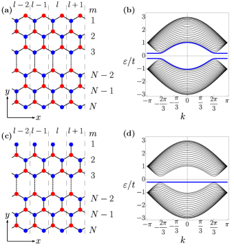
Figure 2: Panel (a) and (c): Gapped graphene nanoribbon with zig-zag boundaries on both edges and a zig-zag and a bearded edge (at the top), respectively. Red (blue) discs signify atoms of the $\sigma=A$ ($\sigma=B$) sublattice, $l$ labels the unit cells, $m$ the rows in each unit cell. Panel (b) and (d): Band structures of nanoribbons of panels (a) and (c), respectively, for $N=20$ and $\Delta=0.2t$. Non-topological edge states are depicted by blue lines.

Example: “gapped graphene”—To demonstrate the main features of the general theory developed above, we calculate the valley Hall current and the valley density accumulation rate for a nanoribbon of “gapped graphene”—a model system that captures some aspects of monolayer graphene on a gap-inducing hBN substrate. Lattice sites are labelled with a unit cell number $l$ and a composite index $(m,\sigma)$, where $m=1,\dots,N$ denotes the row, while $\sigma=A,B$ distinguishes the sublattice within a given row. The $y$ coordinate will be assumed to take integer values to mark the position within a row and half-integer values to mark the position in between the rows. The two sublattices, $A$ and $B$, have different on-site potentials $\pm\Delta$. Electrons are assumed to hop only between nearest neighbors. We neglect spin-orbit interaction and therefore consider spinless electrons.

For the nanoribbon we consider two terminations: a) zig-zag boundaries on both edges [Fig. 2(a)] and b) a zig-zag and a bearded edge [Fig. 2(c)]. These lattice terminations ensure that the valley number is conserved by the unperturbed Hamiltonian. Each unit cell consists of $N$ horizontal rows, with two atoms in each row as shown in Fig. 2(a), except the edge rows, where one atom may be missing as shown in Fig. 2(c).

The band structures for the two terminations, shown in Figs. 2(b) and (d), respectively, feature two bands separated by a gap equal to $2|\Delta|$ with minima at $k=\pm 2\pi/3$. These points define the two valleys in the one-dimensional Brillouin zone. When the lattice is terminated with zig-zag boundaries on both edges, two dispersionless bands of edge states [blue lines in Fig. 2(b)] connect the two valleys and become bulk states for $|k|<2\pi/3$. The upper (lower) band of edge states resides on the upper (lower) edge in Fig. 2 (a).

Our main results are presented in Fig. 3. For a Fermi energy in the gap ($\varepsilon_{\rm F}=0$) and at zero temperature, we find that $n_{v}(m,0)=0$ for either termination, consistent with the fact that there are no states at the Fermi level. At the same time $j^{y}_{v}(m+1/2,0)=-Ee^{2}\cdot\mbox{sign}(\Delta)/(2\pi)+O(\Delta/t)$ for $1\leq m\leq N-1$ as shown in panel (a), blue line: this is the undergap current associated with the nearly-quantized Hall conductance (the actual value $-0.9$ deviates from the ideal quantized value $-1$ due to the finite bandwidth of the model) [26].

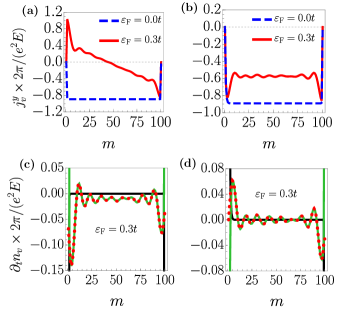
Figure 3: Panel (a): Gapped graphene nanoribbon with zig-zag edges: the blue dashed line shows the valley Hall current as a function of position at Fermi energy $\varepsilon_{\rm F}=0$ and the red solid line shows the same quantity at $\varepsilon_{\rm F}=0.3t$ Panel (b): Same as in (a) for a nanoribbon with one edge zig-zag and the other bearded. Panel (c): The green line shows the valley density accumulation rate contributed by the valley Hall current in the doped nanoribbon with zig-zag edges. The black line shows the contribution of the non-conservation term, and the red dotted line is the sum of the two, i.e., the total accumulation rate. Panel (d): Same as in (c) for the nanoribbon with one zig-zag and one bearded edge. In all plots $N=100$, $\Delta=0.1t$. In plots (c) and (d) $\varepsilon_{\rm F}=0.3t$.

When the system is doped with electrons ($\varepsilon_{\rm F}=0.3t$), the current distributions differ dramatically for the two terminations, as shown by the red lines in Figs. 3 (a) and (b). In the case of the double zig-zag termination the current shows a linear variation across the ribbon (red line in (a)), changing sign about the center of the ribbon. This behavior is completely at odds with our intuition, which would lead us to expect an approximately constant current in the bulk, but not entirely unexpected, because there is no scattering and electrons propagate ballistically. Of greater physical interest, however, is the valley density accumulation rate which is shown in Fig. 3 (c). There is a significant cancellation between $-\partial_{y}j_{v}^{y}$ (green line) and the non-conservation term (black line) at the edges. The sum of the two results in a density accumulation rate which displays oscillations (red dots) on the scale of half the Fermi wavelength and two spikes of equal signs at the edges. These are the result of interference between the electronic waves incident on and reflected off the edge. The fact that the accumulation rate does not integrate to zero is the result of the anomaly on the right-hand side of Eq. (5): valley number is pumped from one valley into the other via a partially filled band of edge states connecting the two (upper blue line in Fig. 2 (b)). This opens the way to an intriguing possibility of generating a net valley density polarization by purely electrical means, as opposed to the standard optical methods. Notice, however, that the form of valley density accumulation rate cannot be predicted from the valley Hall current alone and depends on the boundary conditions.

The zig-zag+bearded termination presents us with a more familiar scenario. Panel (b) of Fig. 3 shows that the valley Hall current is approximately constant ($-0.55$ in units of $e^{2}E/(2\pi)$ at $\varepsilon_{\rm F}=0.3t$) in the bulk. At the same time the valley density accumulation rate, presented in panel (d) has spikes of opposite signs on the two edges. This suggests a more conventional picture of valley density being transported from one edge to the other. The reason for the overall valley number conservation is, in contrast to the previous example, absence of any partially filled bands that would connect the two valleys.

Conclusion—The modified continuity equation (1) allows us to explain how a non-vanishing undergap valley current can coexist with a vanishing valley density accumulation in a fully gapped non-topological time-reversal-invariant system with perfectly degenerate valleys. Any valley density accumulation requires the existence of states at the Fermi level and furthermore it is a dissipative process which requires a scattering mechanism to reach a steady state. We have provided closed expressions for calculating valley density accumulation rates on the edges of a two-dimensional material and we have applied them to the gapped graphene model: these formulas show that the connection between bulk currents and measurable edge accumulations is much more complex than previously suspected. This, in particular, leads us to surmise that any physical system in which evidence of the VHE has been found either by Kerr rotation microscopy [11] or by non-local resistance measurements [1, 16, 17, 18, 19] cannot be a true insulator but must have partially populated bulk or edge states.

Acknowledgments—A.P. acknowledges support from the European Commission under the EU Horizon 2020 MSCA-RISE-2019 programme (project 873028 HYDROTRONICS). A.P. and A.K. acknowledge support from the Leverhulme Trust under the grant RPG-2019-363. H.S. and G.V. were supported by the Ministry of Education, Singapore, under its Research Centre of Excellence award to the Institute for Functional Intelligent Materials (I-FIM, project No. EDUNC-33-18-279-V12).

References

- Gorbachev et al. [2014] R. V. Gorbachev, J. C. W. Song, G. L. Yu, A. V. Kretinin, F. Withers, Y. Cao, A. Mishchenko, I. V. Grigorieva, K. S. Novoselov, L. S. Levitov, and A. K. Geim, Science 346, 448 (2014).
- Zhu et al. [2017] M. J. Zhu, A. V. Kretinin, M. D. Thompson, D. A. Bandurin, S. Hu, G. L. Yu, J. Birkbeck, A. Mishchenko, I. J. Vera-Marun, K. Watanabe, T. Taniguchi, M. Polini, J. R. Prance, K. S. Novoselov, A. K. Geim, and M. Ben Shalom, Nature Communications 8, 14552 (2017).
- Lensky et al. [2015] Y. D. Lensky, J. C. W. Song, P. Samutpraphoot, and L. S. Levitov, Phys. Rev. Lett. 114, 256601 (2015).
- Xiao et al. [2007] D. Xiao, W. Yao, and Q. Niu, Phys. Rev. Lett. 99, 236809 (2007).
- Beconcini et al. [2016] M. Beconcini, F. Taddei, and M. Polini, Phys. Rev. B 94, 121408 (2016).
- Song and Vignale [2019] J. C. W. Song and G. Vignale, Phys. Rev. B 99, 235405 (2019).
- Marmolejo-Tejada et al. [2018] J. M. Marmolejo-Tejada, J. H. García, M. D. Petrović, P.-H. Chang, X.-L. Sheng, A. Cresti, P. Plecháč, S. Roche, and B. K. Nikolić, Journal of Physics: Materials 1, 015006 (2018).
- Roche et al. [2022] S. Roche, S. R. Power, B. K. Nikolić, J. H. García, and A.-P. Jauho, Journal of Physics: Materials 5, 021001 (2022).
- Aktor et al. [2021] T. Aktor, J. H. Garcia, S. Roche, A.-P. Jauho, and S. R. Power, Phys. Rev. B 103, 115406 (2021).
- Bhowal and Vignale [2021] S. Bhowal and G. Vignale, Phys. Rev. B 103, 195309 (2021).
- Lee et al. [2016] J. Lee, K. F. Mak, and J. Shan, Nature Nanotechnology 11, 421 (2016).
- Du et al. [2022] W. Du, R. Peng, Z. He, Y. Dai, B. Huang, and Y. Ma, npj 2D Materials and Applications 6, 11 (2022).
- Ma et al. [2020] X. Ma, X. Shao, Y. Fan, J. Liu, X. Feng, L. Sun, and M. Zhao, J. Mater. Chem. C 8, 14895 (2020).
- Zhou et al. [2019] B. Zhou, Z. Li, J. Wang, X. Niu, and C. Luan, Nanoscale 11, 13567 (2019).
- Mak et al. [2014] K. F. Mak, K. L. McGill, J. Park, and P. L. McEuen, Science 344, 1489 (2014).
- Sui et al. [2015] M. Sui, G. Chen, L. Ma, W.-Y. Shan, D. Tian, K. Watanabe, T. Taniguchi, X. Jin, W. Yao, D. Xiao, and Y. Zhang, Nature Physics 11, 1027 (2015).
- Endo et al. [2019] K. Endo, K. Komatsu, T. Iwasaki, E. Watanabe, D. Tsuya, K. Watanabe, T. Taniguchi, Y. Noguchi, Y. Wakayama, Y. Morita, and S. Moriyama, Applied Physics Letters 114, 243105 (2019), https://pubs.aip.org/aip/apl/article-pdf/doi/10.1063/1.5094456/13307549/243105_1_online.pdf .
- Shimazaki et al. [2015] Y. Shimazaki, M. Yamamoto, I. V. Borzenets, K. Watanabe, T. Taniguchi, and S. Tarucha, Nature Physics 11, 1032 (2015).
- Arrighi et al. [2023] E. Arrighi, V. H. Nguyen, M. D. Luca, G. Maffione, Y. Hong, L. Farrar, K. Watanabe, T. Taniguchi, D. Mailly, J. C. Charlier, and R. Ribeiro-Palau, Non-identical moiré twins in bilayer graphene (2023), arXiv:2205.01760 [cond-mat.mes-hall] .
- Lyalin et al. [2023] I. Lyalin, S. Alikhah, M. Berritta, P. M. Oppeneer, and R. K. Kawakami, APS Bulletin (2023).
- Note [1] Edges are chosen to be parallel to the separation of the valleys in momentum space in such a way that the valley index is a good quantum number in the absence of the electric field and impurities.
- Note [2] The Bloch momentum (modular momentum) operator in a lattice is defined by the identity , where is the ordinary momentum operator and an integer. The operator is well defined because , a periodic function of over the Brillouin zone, is expandable in a series of plane waves of the form .
- Note [3] A similar situation was discussed in Ref. [Shi_prl_2006] for the spin current in the spin Hall effect, with the crucial difference that the non-conservation of the spin density was caused, in that case, by the intrinsic spin-orbit torque, while in our case it is caused by the very same electric field that drives the valley Hall effect.
- Kubo [1957] R. Kubo, Journal of the Physical Society of Japan 12, 570 (1957).
- Giuliani and Vignale [2005] G. Giuliani and G. Vignale, Quantum Theory of the Electron Liquid (Cambridge University Press, 2005).
- Note [4] See the supplemental online material for more details.