Progressive Learning with Cross-Window Consistency for Semi-Supervised Semantic Segmentation

Abstract

Semi-supervised semantic segmentation focuses on the exploration of a small amount of labeled data and a large amount of unlabeled data, which is more in line with the demands of real-world image understanding applications. However, it is still hindered by the inability to fully and effectively leverage unlabeled images. In this paper, we reveal that cross-window consistency (CWC) is helpful in comprehensively extracting auxiliary supervision from unlabeled data. Additionally, we propose a novel CWC-driven progressive learning framework to optimize the deep network by mining weak-to-strong constraints from massive unlabeled data. More specifically, this paper presents a biased cross-window consistency (BCC) loss with an importance factor, which helps the deep network explicitly constrain confidence maps from overlapping regions in different windows to maintain semantic consistency with larger contexts. In addition, we propose a dynamic pseudo-label memory bank (DPM) to provide high-consistency and high-reliability pseudo-labels to further optimize the network. Extensive experiments on three representative datasets of urban views, medical scenarios, and satellite scenes demonstrate our framework consistently outperforms the state-of-the-art methods with a large margin. Code will be available publicly.

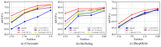
Figure 1: Performance (mean intersection-over-union, mIOU) comparisons between our framework and the state-of-the-art methods on various datasets from multiple fields: (a) urban street scenes segmentation (i.e. , Cityscapes [9]), (b) medical nuclear segmentation (i.e. , MoNuSeg [29]), and (c) land cover classification (i.e. , DeepGlobe [10]). It is worth noting that our method (red lines) surpasses existing methods significantly on various datasets under different partition protocols. Methods studied: SupOnly (supervised baseline), CutMix [56], CPS [8], CAC [31], ST++ [53], UniMatch [52], and the proposed framework. See Section 4 for experiment details.

1 Introduction

Semantic segmentation, as a fundamental and essential task, is widely employed in a wide range of situations, such as automated driving, medical pathology diagnosis, and land cover survey [57, 41, 47]. The brilliant performance of data-driven deep learning algorithms largely depends on huge volumes of annotated data. In practice, massive unlabeled images are collected, but it is hard to acquire the corresponding pixel-level annotations. Despite the availability of advanced semi-automatic labeling algorithms [33, 18], the process of generating annotated data is still tremendously labor-intensive and time-consuming, particularly the annotating process of remote sensing and medical images requires the participation of experts with domain knowledge. To alleviate this issue, numerous semi-supervised learning methods [45, 40, 8, 53, 34, 13, 49, 46] have been developed and achieve promising performance.

Although lots of achievements have been obtained in semi-supervised semantic segmentation, many tricky challenges still remain. The first challenge is how to generate or select pseudo-labels with high-reliability for preventing catastrophic performance degradation. Minimizing the adverse impact of the noise of pseudo-labels is a longstanding but unsolved issue in self-training pipelines [53]. The second challenge is that heterogeneous consistency traits are not fully utilized. Contextual-aware consistency [31] can be viewed as a unique form of data augmentation (i.e. , contextual augmentation) and applied to unlabeled data. Similar ideas are also involved in self-supervised learning [3] and image-to-image translation [28], which shows that cross-window consistency (CWC) is promising. However, it is still insufficient for existing works to fully exploit the merit of CWC. For instance, Directional Contrastive loss from [31] requires manual setting of some key parameters (such as the positive filtering threshold) that must be tuned depending on the datasets. As a whole, CWC is preliminarily explored in the consistency loss modeling, but unfortunately ignored in the selection of high-quality pseudo-labels.

Similar to the peripheral vision system in human vision [32, 35], human visual reasoning processes need to rely on multiple contour regions that cover different contextual information. In life, when humans view images from cross windows, the visual center of the cerebral cortex often produces the same response on overlapping regions. These facts guide us to leverage CWC to exploit unlabeled data.

In light of the aforementioned challenges and the inspiration of human vision, we propose a progressive learning framework on the fundamental idea that overlapping regions on image patches from diverse contextual windows exhibit semantic consistency, systematically exploiting the benefits of this inherent consistency. Our framework progressively optimizes deep network by mining weak-to-strong constraints from unlabeled data. Specifically, in the first stage, we introduce a general and effective biased cross-window consistency (BCC) loss that measures the semantic consistency of overlapping regions based on the segmentation confidence maps. In the second stage, we further extend this fundamental concept by designing a unique pseudo-label reliability evaluating method and establishing a highly dynamic and rewarding dynamic pseudo-label memory bank (DPM) to assist in exposing the model to strong pseudo-label constraints. Benefiting from our proposed pseudo-label reliability evaluation algorithm guided by the inherent cross-window dependencies of images and a well-designed DPM, our approach does not compute the pseudo-label discrepancy of the model at multiple phases as in ST++ [53], but instead only computes the contextual prediction consistency of overlapping regions in different windows to to ensure the information in the DPM is constantly and dynamically updated.

Our framework is generalized and can be extended simply to semi-supervised semantic segmentation applications (e.g. , urban street scenes segmentation in computer vision, medical nuclear segmentation in pathological analysis, and land cover classification in remote sensing). Extensive experiments on the Cityscapes [9], MoNuSeg [29], and DeepGlobe [10] datasets demonstrate a considerable performance improvement over the state-of-the-art methods, as shown in Figure 1. By systematically exploring CWC, our main contributions are summarized as follows:

• The BCC loss with the importance factor is designed to maintain larger contextual semantic consistency among overlapping confidence maps.

• We propose a DPM using a novel pseudo-label reliability evaluation method to minimize the adverse effects of ill-posed pseudo-labels.

• Our framework outperforms previous methods on extensive datasets from different fields, which demonstrates the strong generalization and competitiveness of our work.

2 Related Work

Semi-supervised semantic segmentation‘s crux and core is how to properly utilize unlabeled data and be able to further enhance the generalization of the model with less labeled data. With the rapid improvement of semi-supervised learning (SSL) methods [44, 16, 59, 37, 2], solutions based on different paradigms have made progress in semi-supervised semantic segmentation tasks. The current semi-supervised semantic segmentation approach consists of three typical pipelines: GAN-based, self-training, and consistency regularization methods. In semi-supervised semantic segmentation, GANs [15, 36] are used as discriminative tools or supervised signals alone or in conjunction with other methods. For example, Hung et al. [24] uses discriminators of GAN networks to find pseudolabeled plausible regions. Previous works [36, 22] add the GAN branch as an auxilary supervision in natural and medical images, respectively.

Consistency regularization-based methods make features of samples from the same category more compact in the feature space, while keeping features of samples from different categories as far as possible. The benefit comes in the implement’s flexibility, which includes the design and metrics of consistency traits. Specifically, CutMix [56], ClassMix [38], and various other data augmentations [42] are federated in the consistency regularization framework in order to transform or perturb the input data to satisfy the constraints of the consistency measure, just as [40, 34] do. Similarly, further broader disturbances and different initialization model are published to achieve a gain [13, 8], respectively. Contrastive loss that performs well on other tasks is relocated to the consistency regularization paradigm in owing to the rapid advancement of contrastive learning and self-supervised learning [54, 26, 19, 7]. For instance, InfoNCE [39], which attempts to bring positive pairs closer and push negative pairs apart and shines in self-supervised learning, has been extensively modified and adapted to many previous methods [58, 51, 31, 49, 50]. In addition, CCT [40] emphasizes the validity of the mean square error (MSE) as an elegant consistency loss.

Self-training-based and Pseudo labeling-based methods commonly leverage student-teacher models to produce and re-train pseudo-labels. Chronic challenges include how to generate or select pseudo-labels with high-confidence to optimize the model and tackle the class-imbalanced issue. In response to the first problem outlined, ST++ [53] proposes a straightforward yet effective pipeline that boosts model stability through strong and weak data transformations and by gradually utilizing all pseudo-labels. Instead of ignoring the doubtful pixels of pseudo-labels, U²PL [48] treats them as negative samples to be compared with the matching positive samples. ELN [30] and Yuan et al. [55] create the ELN module to correct pseudo labels and self-correction loss to prevent overfiting to the noise of low-confidence pseudo-labels, respectively. The class-imbalance bias of pseudo-labels undermine the generalization of the model, particularly when there are very few unlabeled samples or when the sample contains a significant long-tail effect. Numerous solutions [17, 23, 21] recognize this issue and align class distributions to rectify the imbalance. Note that the existing methods do not perfectly address the mentioned challenges.

Different from previous methods, our framework focuses on exploring CWC and brings significant performance gain by minimizing differences among unlabeled data across diverse windows to mitigate cross-window bias and dynamically selecting rewarding pseudo-labels to avoid the misleading of ill-posed pseudo-labels and overfitting of fixed pseudo-labels.

3 Method

3.1 Problem Definition

The goal of semi-supervised semantic segmentation is to employ a small set of labeled data $\mathcal{B}_{l}=\left\{\left(x_{i},y_{i}\right)\right\}_{i=1}^{M}$ with unlabeled data $\mathcal{B}_{u}=\left\{u_{i}\right\}_{i=1}^{N}$ to train a model $\mathcal{F}$ that can provide accurate results on test data. In general, the overall optimization loss can be formulated as:

$$\mathcal{L}_{total}=\mathcal{L}_{s}+\lambda\mathcal{L}_{u},$$ (1)

where $\lambda$ is a trade-off weight between labeled and unlabeled data supervision. Typically, the labeled supervised loss $\mathcal{L}_{s}$ is the cross-entropy loss or correlation variant (e.g. , OHEM [43]) of the inferences and annotated labels. The unsupervised loss $\mathcal{L}_{u}$ can be defined flexibly as consistency loss, pseudo-label loss, entropy minimum loss, etc. , thereby encouraging the model to fit the unlabeled data.

3.2 Motivation and Overview

The majority of existing consistency regularization-based approaches [40, 58, 50, 51] focus on learning feature consistency following perturbation or data augmentation, whereas CAC [31] introduces a context-aware consistency loss that compares high-level feature consistency. In contrast to it, (1) we focus on the fact that the feature representation computation is unstable (even with the participation of the feature projection [5]), and (2) we apply the spontaneous existing image CWC traits to filter pseudo-labels, and subsequent experiments demonstrate its effectiveness, as highlighted in Figure 2.

Figure 2: Emphasize the differences between our approach and previous work. In contrast to (a) CAC [31], we employ the stable confidence maps rather than feature maps to encourage consistency of overlapping regions from wider contextual windows, and further apply CWC traits to select high-reliability pseudo-labels. (c) SAC [1], which is designed for domain adaptation, is to enforce consistency of the semantic maps created by the model across image perturbations rather than utilizing the consistency of overlapping regions across windows as we do.

Motivated by the aforesaid discussions, our overall optimization objective function can be defined as follows:

$$\mathcal{L}_{total}=\mathcal{L}_{s}+\lambda_{BCC}\mathcal{L}_{BCC}+\lambda_{DPM}\mathcal{L}_{DPM},$$ (2)

$$\mathcal{L}_{s}=\frac{1}{\left|\mathcal{B}_{l}\right|}\sum\limits_{\mathbf{X}\in\mathcal{B}_{l}}\frac{1}{W\times H}\sum\limits_{i=0}^{W\times H}\left(\ell_{ce}\left(\mathbf{p}_{i},y_{i}\right)\right),$$ (3)

where $W$ and $H$ represent the width and height of images. For the labeled dataset $\mathcal{B}_{l}$, the semantic segmentation model $\mathcal{F}$ is employed to generate its confidence map $\mathbf{p}_{i}$ (after $Softmax$ normalization), which is supervised by the ground truth $y_{i}$ using the cross-entropy loss $\ell_{ce}$ . As for the unlabeled dataset $\mathcal{B}_{u}$, our BCC loss $\mathcal{L}_{BCC}$ reflects the weak constraint, as described in Section 3.3. The pseudo-label supervised loss $\mathcal{L}_{DPM}$ is the strong constraint, and Section 3.4 describes the pseudo-label filtering and usage.

Ideally, all items of the Eq. (2) are optimized together, but it is extremely GPU memory-consuming. To operate pervasively on the overwhelming majority of devices, we propose a progressive learning strategy to achieve the ultimate optimization goal. Algorithm 1 and Figure 3 offer a comprehensive pseudocode description and an intuitive overivew of our whole framework, respectively.

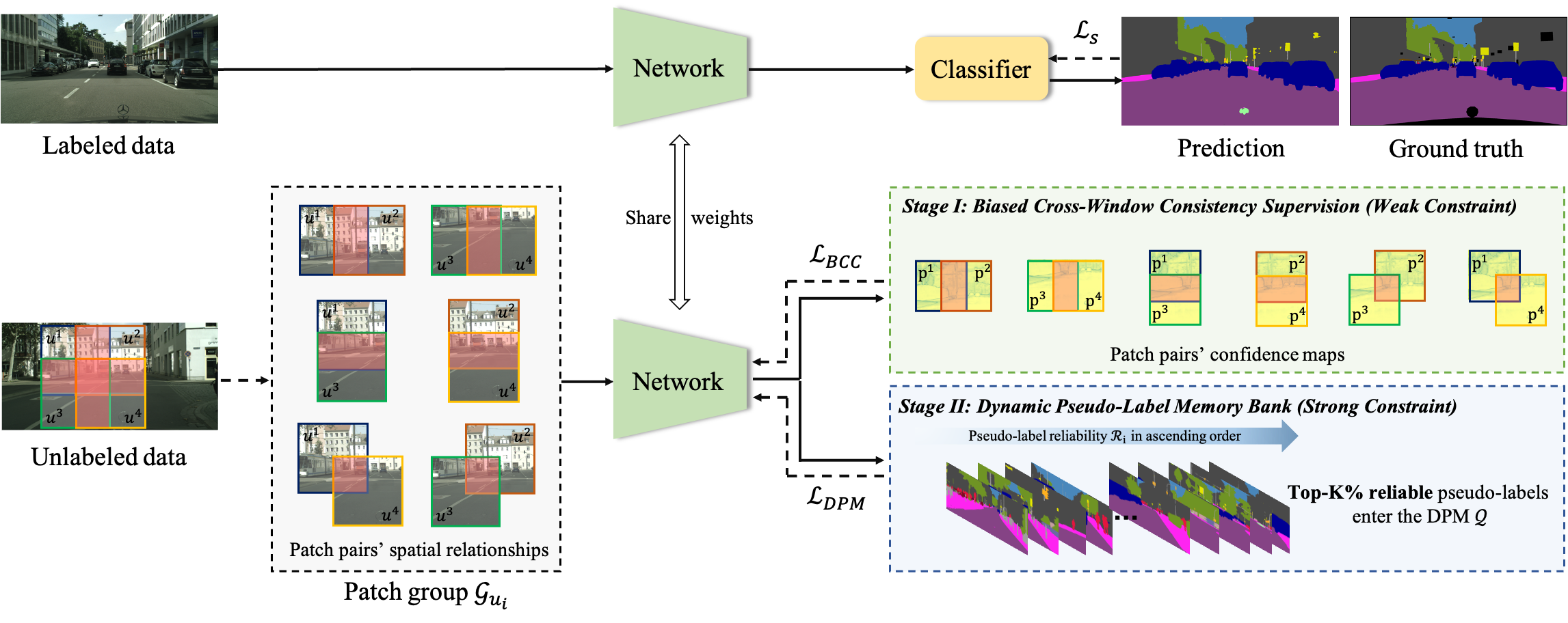
Figure 3: An overview of our proposed framework. labeled data is employed for supervised training the model $\mathcal{F}$. For unlabeled data, in stage I, we present a novel BCC loss with an importance factor (Eq. (LABEL:con:deqn_ex4)) to encourages the model to maintain consistency across overlapping confidence maps in different windows but does not restrict specific class attributes. In addition, we propose the DPM to rank the pseudo-label reliability (Eqs. (7) and (8)) in light of CWC and dynamically update and manage rewarding pseudo-labels.

Algorithm 1 Our Framework Pseudocode

0:  Labeled images and corresponding labels $\mathcal{B}_{l}=\left\{\left(x_{i},y_{i}\right)\right\}_{i=1}^{M}$ Unlabeled images $\mathcal{B}_{u}=\left\{u_{i}\right\}_{i=1}^{N}$Validation set $\mathcal{B}_{v}=\left\{\left(x_{i},y_{i}\right)\right\}_{i=1}^{V}$

0:  Trained model $\mathcal{F}$

1:  #Stage I: Biased Cross-Window consistency supervision (weak constraint)

2:  Train $\mathcal{F}$ on $\mathcal{B}_{l}$ with cross-entropy loss and $\mathcal{B}_{u}$ based on Eq. (LABEL:con:deqn_ex4)

3:  Initialize previous best $\mathcal{S}\leftarrow 0$

4:  Calculate previous best $\mathcal{S}\leftarrow\operatorname{meanIOU}\left(\mathcal{F}\left(\mathcal{B}_{v}\right)\right)$

5:  Initialize count $count\leftarrow 0$

6:  while epoch$<$maximum number of epochs do

7:     #Stage II: Dynamic pseudo-label memory bank (strong constraint)

8:     for $u_{i}$ $\in$ $\mathcal{B}_{u}$ do

9:        Get reliability score $\mathcal{R}_{i}$ based on Eqs. (7) and (8)

10:     end for

11:     Select Top-K% scored unlabeled images and generate corresponding pseudo-labels $y_{i}^{*}$ into the dynamic pseudo-label memory bank $\mathcal{Q}=\left\{\left(u_{i},y_{i}^{*}\right)\right\}_{i=1}^{N\times K\%}$

12:     Train $\mathcal{F}$ on $\mathcal{B}_{l}\cup\mathcal{Q}$ with cross-entropy loss

13:     $count\leftarrow count+1$

14:     Calculate current $\mathcal{S}^{{}^{\prime}}\leftarrow\operatorname{meanIOU}\left(\mathcal{F}\left(\mathcal{B}_{v}\right)\right)$

15:     if $\mathcal{S}^{{}^{\prime}}>\mathcal{S}+\mathcal{G}$ or $count>\mathcal{K}$ then

16:        Update the $\mathcal{Q}$ (Jump to Stage II)

17:        Update previous best $\mathcal{S}\leftarrow\mathcal{S^{{}^{\prime}}}$

18:        Re-initialize count $count\leftarrow 0$

19:     end if

20:  end while

21:  return  $\mathcal{F}$

3.3 Stage I: Biased Cross-Window Consistency Supervision (Weak Constraint)

For each unlabeled image $u_{i}$, four adjacent and overlapping patches (default minimum overlap size is $\frac{H}{2}$ or $\frac{W}{2}$) are defined as a patch group $\mathcal{G}_{u_{i}}=\left\{\left(u_{i}^{1},u_{i}^{2},u_{i}^{3},u_{i}^{4}\right)\right\}_{i=1}^{N}$, and their spatial relationships are depicted in Figure 3. Any patch pairs $\left(u_{i}^{k},u_{i}^{l}\right)$ containing overlapping regions $u_{oi}$ are processed by the encoder $\mathcal{E}$, decoder $\mathcal{D}$, and classifier $\mathcal{C}$ to obtain a $softmax$ normalized confidence map $\mathbf{p}_{i}$, which is then used to calculate the BCC loss.

BCC loss encourages overlapping regions within the pair groups to have semantically consistent representations but does not restrict specific class attributes. In particular, to encourage the model to focus on prominent differences with different semantic classes in overlapping regions, we propose the importance factor $\mathcal{M}_{imp}^{h,w}$ to eliminate insignificant differences (pixel positions with different confidence maps but the same semantic classes), as illustrated in Figure 4. Intuitively, the importance factor $\mathcal{M}_{imp}^{h,w}$ will amplify the difference between the feature information of pixels that are more valuable to the model. Table 4 experimental results demonstrate its benefits. Our BCC loss can be written as

$$\begin{split}&\mathcal{L}_{BCC}=\frac{1}{\left|B_{u}\right|}\sum_{x\in B_{u}}\\ &\frac{1}{W\times H}\sum_{i=0}^{W\times H}\sum_{1\leqslant k<l\leqslant 4}\ell_{2}\left(\mathbf{p}_{oi}^{k},\mathbf{p}_{oi}^{l}\right)\cdot\mathcal{M}_{imp}^{h,w},\end{split}$$ (4)

$$\mathbf{p}_{oi}^{k}=\operatorname{Softmax}\left(\mathcal{C}\left(u_{oi}^{k}\right)\right),$$ (5)

$$\begin{split}&\mathcal{M}_{imp}^{h,w}=\\ &\mathbf{1}\left\{\operatorname{argmax}\left(\mathcal{C}\left(u_{ok}^{h,w}\right)\right)\neq\operatorname{argmax}\left(\mathcal{C}\left(u_{ol}^{h,w}\right)\right)\right\},\end{split}$$ (6)

where $\ell_{2}\left(\mathbf{p}_{oi}^{k},\mathbf{p}_{oi}^{l}\right)=\left\|\mathbf{p}_{oi}^{k}-\mathbf{p}_{oi}^{l}\right\|_{2}^{2}$ calculates the square of the euclidean distance of the confidence maps of the overlapping regions. $W$ and $H$ represent the width and height of output maps. $k$ and $l$ represent the sequence number of spatial relationships among the patch group $\mathcal{G}_{u_{i}}$.

Discussion. $\mathcal{L}_{BCC}$ uses an elegant $\ell_{2}$ for the distance measure between the anchor and positive samples, which ensures the high efficiency of our entire framework. It achieves a 1.7% and 8.98% performance improvement on Cityscapes and MoNuSeg after the joint $\mathcal{M}_{imp}^{h,w}$, respectively. (see Table 4 and the supplementary file.)

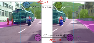
Figure 4: Illustration of the importance factor $\mathcal{M}_{imp}^{h,w}$. It eliminates insignificant differences (pixel positions with different confidence maps but the same semantic classes)

3.4 Stage II: Dynamic Pseudo-Label Memory Bank (Strong Constraint)

To increase the quality of training pseudo-labels and prevent noise from adversely affecting the model. Supported by CWC, we come up with the concept of the DPM $\mathcal{Q}$ for selecting reliable pseudo-labels and dynamically maintaining a high confidence and high consistency pseudo-label repository to undertake pseudo-label supervision.

How to dynamically update? Previous attempts [44] to evaluate the reliability of pseudo-labels mainly focus on pixel-level filtering methods, with the common strategy being to filter out low-confidence pixel information via manual or adaptive thresholding. However, filtered pixels often include complex and vital information, which may increase the negative consequences of the long-tail effect. ST++ [53] presents a method for image-level selection by evaluating the stability of pseudo-labels at various training phases. It needs to calculate the model’s classification differences for numerous phases, which is time-consuming. In our framework, we investigate an efficient algorithm for evaluating the reliability of pseudo-labels in order to promote rewarding updating of DPM $\mathcal{Q}$. Specifically, we reckon that the greater the semantic consistency of pseudo-labels in overlapping regions including patches from different contexts, the greater the reliability of pseudo-labels. Thus, for each unlabeled image $u_{i}$, we randomly crop and form a patch group $\mathcal{G}_{u_{i}}=\left\{\left(u_{i}^{1},u_{i}^{2},u_{i}^{3},u_{i}^{4}\right)\right\}_{i=1}^{N}$ having four adjacent and overlapping patches of size $H_{o}\times W_{o}$. We utilize the model developed currently to evaluate the meanIOU of the predictions of the four patches’ overlapping regions as the reliability score $\mathcal{R}_{i}$.

$$\mathbb{C}_{oi}=\sum_{1\leqslant k<l\leqslant 4}\text{ConfusionMatrix}\left(y_{oi}^{k*},y_{oi}^{l*}\right),$$ (7)

$$\mathcal{R}_{i}=\operatorname{meanIOU}\left(\mathbb{C}_{oi}\right),$$ (8)

where $y_{oi}^{k*}=\operatorname{argmax}\left(\mathcal{C}\left(u_{oi}^{k}\right)\right)$ is pseudo masks of overlapping regions $u_{oi}$. After getting the reliability scores of all unlabeled images, we sort the entire set of unlabeled images based on these scores and select the Top-K% reliable images pseudo-labels and corresponding images to entry into the DPM $\mathcal{Q}$. (The original pseudo-labels in the DPM will be totally replaced.)

When will an update be made? To maintain the optimal pseudo-labels in the DPM at all times, the DPM will be automatically updated when the model achieves a gain of $\mathcal{G}$ on the validation set or when it reaches a predefined $\mathcal{K}$ epochs of training. This ensures that the model always obtains more rewarding information from the DPM.

We employ pseudo-labels $y_{ui}^{*}$ from the DPM to rigorously supervise the confidence map $\mathbf{p}_{ui}$ of the corresponding model output using cross-entropy loss:

$$\mathcal{L}_{DPM}=\frac{1}{\left|\mathcal{B}_{u}\right|}\sum\limits_{\mathbf{X}\in\mathcal{B}_{u}}\frac{1}{W\times H}\sum\limits_{i=0}^{W\times H}\left(\ell_{ce}\left(\mathbf{p}_{ui},y_{ui}^{*}\right)\right),$$ (9)

where $W$ and $H$ represent the width and height of unlabeled images, respectively.

Discussion. Instead of always utilizing all unlabeled images and corresponding pseudo-labels [12], our DPM dynamically filters out the less-reliable pseudo-labels based on CWC. In addition, our DPM updates information more frequently and flexibly in order to assist the model in learning more rewarding unlabeled data. The experimental results listed in Table 4 and Figure 5 demonstrate its benefits.

4 Experiments

4.1 Setup

Datasets. We evaluate our approach on three publicly available benchmarks to encompass various application scenarios such as urban street scenes semantic segmentation, histopathological tissue detection, and land cover classification, represented by Cityscapes [9], MoNuSeg [29], and DeepGlobe [10]. Cityscapes contains 2975 training images with fine-annotated labels of 19 semantic classes and 500 validation images. We compare our method with state-of-the-art methods under 1/30, 1/16, 1/8, and 1/4 partition protocols following ST++ [53] and CPS [8]. MoNuSeg was published by the multi-organ nuclei segmentation challenge [29] and consists of 30, 7, and 14 histopathologic images ($1000\times 1000$ pixels) for training, validation, and testing, respectively. Our and other methods are implemented under 1/30, 1/6, 1/3, and full supervision partition protocols. DeepGlobe contains 803 satellite images ($2448\times 2448$ pixels) that are applied for land cover classification analysis in the field of remote sensing. Following [6], we divide the images into the training set, validation set, and test set with 454, 207, and 142 images, respectively. Similarly, our and other methods are implemented under 1/16, 1/8, 1/4, and full supervision partition protocols.

Evaluation. We employ DeepLabv3+ [4] with ResNet-50 [20] that has been pre-trained on ImageNet [11] as our segmentation model to ensure a fair comparison with prior work. (Experiments based on DeepLabv3+ with ResNet-101 are displayed in the supplementary file.) We use the mean intersection-over-union (mIOU) metric to evaluate the segmentation performance of all datasets, following previous work. For a comprehensive evaluation of MoNuSeg, we also used Dice coefficient (DC), Jaccard coefficient (JC), Specificity (SP), and Sensitivity (SE), which are commonly used in biomedical segmentation. We report results on the 500 Cityscapes val set, the 14 MoNuSeg test set, and the 142 DeepGlobe test set using only single-scale testing and without any post-processing techniques.

Implementation details. The batch-size for all datasets with a single NVIDIA TITAN RTX GPU is set to 2 in Stage I and 4 in Stage II. The initial learning rate of Stage I of the backbone is 0.005, 0.004, and 0.005 for Cityscapes, MoNuSeg, and DeepGlobe, respectively, whereas the learning rate of the segmentation head is 10 times that of the backbone. The initial learning rate of Stage II is reduced to 0.003, 0.003, and 0.004. We use the SGD optimizer to train Cityscapes, MoNuSeg, and DeepGlobe for 280, 200, and 150 epochs under a poly learning rate scheduler, respectively. Following ST++ [53], the labeled data is randomly flipped and resized between 0.5 and 2.0, and the unlabeled images are augmented with colorjitter, grayscale, and blur. Due to memory limitations, we train the model with a smaller crop size than CPS [8] (720 for Cityscapes and 512 for MoNuSeg and DeepGlobe). To get a fair comparison result for Cityscapes, we employ OHEM loss with the same parameters as previous work. For MoNuSeg and DeepGlobe, we train all models using only standard cross-entropy loss, without Sync-BN [25] and auxiliary loss. Moreover, the trade-off weights $\lambda_{BCC}$ and $\lambda_{DPM}$ are set to 0.16 and 1.0, respectively. And the selection of reliable pseudo-labels in Stage II selects, by default, the top 50% of data for storage in the DPM. When the validation set metric achieves a 2% gain or $count$ reaches 25, the DPM is automatically updated with more trustworthy pseudo-labels.

4.2 Comparison with State-of-the-Art Methods

An innovative framework based on the CWC traits of images is proposed. In this section, we implement advanced methods on various datasets with the same segmentation network and setting to ensure the fairness of comparison.

Method	Publication	1/30 (100)	1/16 (186)	1/8 (372)	1/4 (744)
SupOnly†	-	55.1	61.8	66.2	72.3
CPS [8]	CVPR’21	-	69.8	74.4	76.9
CAC [31]	CVPR’21	60.9	69.4	74.0	-
DARS [21]	ICCV’21	-	66.9	73.7	-
ST++† [53]	CVPR’22	61.4	70.1	73.2	74.7
U2PL [48]	CVPR’22	59.8	-	73.0	76.3
USRN [17]	CVPR’22	-	71.2	75.0	-
PS-MT [34]	CVPR’22	-	-	74.4	75.2
CPCL [14]	TIP’23	-	69.9	74.6	77.0
UniMatch [52]	CVPR’23	64.5	-	75.6	77.4
Ours	-	67.3	72.8	76.6	77.6

Table 1: Comparison with state-of-the-art methods on Cityscapes val set under different partition protocols. We use DeepLabv3+ as the segmentation network and ResNet-50 as the backbone. “SupOnly” means supervised training without using any unlabeled data. $\dagger$ means we reproduce the approach and other results are collected from [8, 17, 34]. The best results are marked in bold and the second best ones are marked in italic bold.

Cityscapes. Table 1 shows the results of our method compared with other state-of-the-art methods on the Cityscapes dataset. We reproduce the representative methods within the same network and setting according to their publicly available codes or use the results reported in the original papers. Our framework achieves a stable improvement under different partition protocols. Specifically, our framework outperforms the supervised baseline (SupOnly) by +12.2%, +11.0%, +10.4%, and +5.3% under 1/30, 1/16, 1/8, and 1/4 partition protocols, respectively. Besides, ours outperforms new state-of-the-art methods with larger margins by 2.8% , 1.6%, and 1.0% in mIOU for 1/30, 1/16, and 1/8 split of Cityscapes. Additionally, the training burden is analyzed in the supplementary file.

MoNuSeg. Table 2 shows the comparison results on the MoNuSeg dataset. Compared with latest and advanced methods, ours surpasses them with large margins under all partition protocols (especially when there are few labeled samples participating in training). The DC gap between the SupOnly on full set (77.82%) and our 1/30 labeled setting result (75.51%) is only 2.31%. Under the 1/6 labeled setting, ours outperforms the supervised baseline on the full set (79.62% vs. 77.82%). We also observe that even under full supervision, our framework still obtains a +3.18% gain.

Partition	Method	DC (%)	mIOU (%)	JC (%)	SP (%)	SE (%)
1/30 (1)	SupOnly	61.87	60.13	45.54	79.23	82.32
	CutMix [56]	65.35	64.89	48.75	86.16	75.32
	ST++ [53]	68.68	67.05	52.49	85.83	81.30
	UniMatch [52]	63.77	63.51	47.15	85.22	75.42
	Ours	75.51	74.46	60.89	92.06	79.47
1/6 (5)	SupOnly	73.16	71.95	58.52	89.20	84.53
	CutMix [56]	74.71	73.77	59.91	90.62	83.96
	CAC [31]	74.10	73.40	59.21	91.72	79.17
	ST++ [53]	77.85	76.46	63.83	92.37	84.60
	UniMatch [52]	74.96	75.32	60.43	97.48	66.54
	Ours	79.62	78.62	66.28	95.72	77.65
1/3 (10)	SupOnly	74.53	72.72	60.07	88.38	87.89
	CutMix [56]	76.72	76.07	62.73	92.62	82.44
	CAC [31]	74.43	74.80	59.63	94.19	73.62
	ST++ [53]	78.41	77.27	64.62	93.72	81.76
	UniMatch [52]	79.15	77.84	65.63	93.51	83.72
	Ours	80.37	78.48	67.27	92.35	88.29
Full (30)	SupOnly	77.82	76.82	64.20	92.59	83.89
	CutMix [56]	78.13	77.03	64.50	92.40	85.09
	CAC [31]	80.71	79.35	67.73	94.38	83.72
	ST++ [53]	79.98	78.80	66.79	94.27	82.54
	UniMatch [52]	78.15	77.31	64.33	94.31	79.66
	Ours	81.00	79.73	68.18	94.75	83.04

Table 2: Comparison with state-of-the-art methods on MoNuSeg test set under different partition protocols. All methods are reproduced by us via DeepLabv3+ with ResNet-50 for a fair comparison.

DeepGlobe. We show the comparison results for the DeepGlobe dataset in Table 3. Ours brings significant and stable improvements compared to the SupOnly and other popular advanced methods under all partition protocols. Besides, the mIOU gap between the SupOnly on full set (68.64%) and our 1/4 labeled setting result (68.51%) is only 0.13%.

Method	Publication	1/16 (28)	1/8 (56)	1/4 (113)	Full* (454)
SupOnly	-	55.47	62.19	66.82	68.64
CutMix [56]	ICCV’19	53.33	61.46	66.07	66.59
CAC [31]	CVPR’21	56.47	62.23	66.26	69.45
ST++ [53]	CVPR’22	55.61	62.21	65.67	69.25
Ours	-	58.36	65.17	68.51	70.01

Table 3: Comparison with state-of-the-art methods on DeepGlobe test set under different partition protocols. All methods are reproduced by us via DeepLabv3+ with ResNet-50 for a fair comparison. * means only using the BCC supervision (Stage I), and discussions about the full data setting are presented in Section 5.

4.3 Ablation Studies

The notable contributions of our framework are condensed into 1) BCC loss with the importance factor, 2) an efficient method for evaluating reliability of pseudo-labels, and 3) the DPM. We conduct our ablation studies with DeepLabv3+ and ResNet-50 on the 1/8 split of Cityscapes to verify the effectiveness of them.

Effectiveness of the BCC loss. In Table 4, we show the outcomes of the naive consistency loss (Exp. I) and our proposed BCC loss $\mathcal{L}_{BCC}$ with the importance factor $\mathcal{M}_{imp}^{h,w}$ (Exp. II), demonstrating that the importance factor $\mathcal{M}_{imp}^{h,w}$ can provide a +1.7% gain over the supervised baseline method (Exp. SupOnly) with only labeled data. And the performance of the model declines (-1.5%) when $\mathcal{L}_{BCC}$ is not used in the first stage of training (Exp. VII). They indicate that BCC loss encourages overlapping regions to maintain prominent semantic consistency. More ablation studies about different overlap sizes and number of patch pairs involved are discussed in the supplementary file.

ID	$\mathcal{L}_{BCC}$ (w/o $\mathcal{M}_{imp}^{h,w}$ )	$\mathcal{L}_{BCC}$ (w/ $\mathcal{M}_{imp}^{h,w}$ )	Random select (50%)	Reliable select (50%)	All unlabeled data	DPM $\mathcal{Q}$	mIOU(%)
SupOnly							66.2
I	✔						66.5
II		✔					67.9
III		✔	✔				71.7
IV		✔		✔			73.0
V		✔			✔		73.1
VI		✔	✔			✔	73.8
VII				✔		✔	75.1
Ours		✔		✔		✔	76.6

Table 4: Ablation study on the effectiveness of various components in our framework. $\mathcal{L}_{BCC}$ : biased cross-window consistency loss, $\mathcal{M}_{imp}^{h,w}$ : importance factor, Random select (50%) means selecting 50% pseudo-labels to retrain randomly. Reliable select (50%) means selecting top-50% reliable pseudo-labels to retrain based on Eqs. (7) and (8). All unlabeled data means using all pseudo-labels to retrain directly. DPM: dynamic pseudo-label memory bank $\mathcal{Q}$.

Minimum overlap size	$\frac{H}{3}$ or $\frac{W}{3}$	$\frac{\textit{{H}}}{\textbf{2}}$ or $\frac{\textit{{W}}}{\textbf{2}}$ (default)	$\frac{2H}{3}$ or $\frac{2W}{3}$
mIOU (%)	67.1	67.9	67.6

Table 5: Ablation study on different minimum overlap sizes. $H$ and $W$ represent the height and width of the input image.

$n$	0	1	3	6 (default)
mIOU (%)	66.2	66.6	66.5	67.9

Table 6: Ablation study on different number of patch pairs in each patch group.

Method	mIOU(%)
Pixel-level filtering	72.5
Our image-level reliability selection	73.0
Ours	76.6

Table 7: Effectiveness of the pseudo-label reliability evaluation. Performance analysis over pixel-level filtering strategy and our image-level reliability selection strategy.

Impact of parameters of the BCC loss. For each unlabeled image $u_{i}$, four adjacent and overlapping patches are defined as a patch group in stage I. And the default minimum overlap size is defined as $\frac{H}{2}$ or $\frac{W}{2}$. The size of the overlapping area determines the difference in the context information contained between adjacent patches. We conduct an ablation study on different minimum overlap sizes, as shown in Table 5, which demonstrates that the most suitable size for $\mathcal{L}_{BCC}$ is $\frac{H}{2}$ or $\frac{W}{2}$.

we further consider $n$ patch pairs with overlapping areas in each patch group. In Table 6, we find that when $n$ reaches the maximum value of 6, the result outperforms other counterparts, which proves that the wider cross-window information involved is beneficial for mining unlabeled data.

Effectiveness of the pseudo-label reliability evaluation. We verify it from two perspectives: (1) as shown in Experiments III and IV in Table 4, the mIOU gap between random selection (50%) and reliable selection (50%) based on Eq. (7) and (8) is 1.3%, indicating that our pseudo-label reliability evaluation is effective. (2) We directly train the model with all unlabeled images and their pseudo-labels, and its performance is nearly identical to that of a model trained with only 50% high-reliable pseudo-labels. This indicates our approach’s capability to reduce noise interference in pseudo-labels, as we mentioned in Section 3.4.

In addition, to further illustrate the advantages of this image-level reliability selection, we implement a comparison with the pixel-level filtering method. Specifically, the pixel-level filtering method ignores the pseudo-label information of the pixels with a maximum class confidence of less than 0.75 during the training phase. As shown in Table 7, our image-level reliability selection is superior to the pixel-level filtering approach.

Efficiency of the pseudo-label reliability evaluation. We employ the same settings and device to make a fair comparison with ST++ [53] on the efficiency of evaluating the reliability of pseudo-labels. ST++ needs to calculate the model’s classification differences for numerous phases. In contrast to ST++ which needs to calculate model classification differences in multiple stages, our method only needs to calculate model differences in overlapping areas in a single stage. In Figure 5(a), the efficiency of the pseudo-label evaluation method based on CWC proposed by us (2.29 FPS) is twice that of ST++ (1.12 FPS), which provides support for the high dynamic performance of DPM.

Effectiveness of the DPM. In Table 4, the comparison between our method’s result and that of Experiment IV demonstrates that the DPM can bring a significant improvement by +3.6%. In addition, the difference between Experiment III and Experiment VI demonstrates the advantage of the DPM even when random selection is employed.

Furthermore, Figure 5(b) illustrates the model performance of the DPM at each automatic update, as well as the renewal ratio of the images corresponding to the memory bank’s pseudo-labels. Specifically, approximately 35% of unlabeled images are changed at each update, demonstrating the high dynamics of the DPM. With the continual update of DPM, our framework’s performance is also continuously enhanced, indicating that it is wise to gradually utilize high-reliability pseudo-labels instead of all pseudo-labels to optimize the model.

We also conduct ablation experiments on the ratio of selected reliable pseudo-labels. The default setting 50% is effective enough, as demonstrated in Table 8.

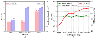
Figure 5: (a) Comparison between the efficiency and accuracy of evaluating the reliability of pseudo-labels. (b) The model performance and the update ratio of the DPM at each automatic update stage. #$k$: the $k$-th update and training. begin: the beginning of Stage II. end: the end of training.

Ratio	20%	50%(default)	80%
mIOU (%)	74.5	76.6	76.3

Table 8: Ablation study on the ratio of reliable pseudo-labels.

4.4 Qualitative results

Figure 6 shows some segmentation results on Cityscapes. We can see that many mis-classified details like truck, sidewalk, and person in the SupOnly and ST++ results are corrected in CWC. More qualitative results on MoNuSeg and DeepGlobe datasets are displayed in the supplementary file.

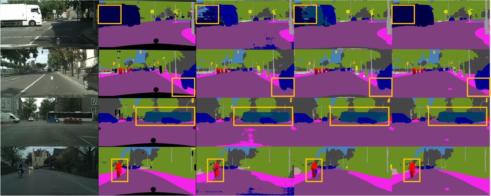
Figure 6: Qualitative results on the Cityscapes set under the 1/8 protocol and ResNet-50 as the backbone. Columns from left to right denote the original images, the ground-truth, the SupOnly results, the ST++ results, and our CWC results, respectively.

5 Discussion about the full data setting

In the full data setting on DeepGlobe dataset, images fed to the unsupervised branch are collected from the labeled training set, as CAC [31] does. Here we add an ablation study on the effect of the varying scale of unlabeled data in the full data setting. Table 9 shows that BCC supervision (Stage I) is also beneficial in the full data setting, and with the increase in the scale of unlabeled data, performance gradually improves. It is recommended to only use Stage I leads to the optimal performance in the full data setting.

Scale	1/16 (28)	1/8 (56)	1/4 (113)	1/2 (227)	Full (454)
SupOnly	-	-	-	-	68.64
Stage I	68.29	68.31	68.63	69.03	70.01 (+1.37)
Stage II	68.13	67.37	66.86	66.11	65.47

Table 9: Results (mIOU%) about the varying scale of unlabeled data in the full data setting on DeepGlobe test set.

6 Conclusion

We propose a progressive learning framework for developing CWC systematically via mining weak-to-strong constraints. At the early stage, we propose a BCC loss with the importance factor to encourage the model to maintain consistency across overlapping confidence maps in different windows but does not restrict specific class attributes. We conceptualize the DPM to dynamically update and manage high-reliability pseudo-labels to strongly constrain the model in the latter period. The evaluation strategy of pseudo-label reliability based on CWC is the key of DPM. Our framework achieves the state-of-the-art performance across three representative datasets from various fields.

Appendix A Comparison of different backbones

Similar to previous methods, we also adopt DeepLabv3+ [4] with ResNet-101 [20] as the segmentation network and conducted experiments on Cityscapes dataset. Results in Table A10 demonstrate that our framework is still effective, without relying on a specific backbone.

Method	Publication	1/16 (186)	1/8 (372)	1/4 (744)
SupOnly†	-	62.2	69.1	72.3
CCT [40]	CVPR’20	69.6	74.5	76.4
GCT [27]	ECCV’20	66.9	73.0	76.5
CPS [8]	CVPR’21	70.5	75.7	77.4
PS-MT [34]	CVPR’22	-	76.9	77.6
ST++† [53]	CVPR’22	70.3	73.9	76.8
Ours	-	74.5	77.0	78.6

Table A10: Comparison with state-of-the-art methods on Cityscapes val set under different partition protocols. We use DeepLabv3+ as the segmentation network and ResNet-101 as the backbone. “SupOnly” means supervised training without using any unlabeled data. $\dagger$ means we reproduce the approach and other results are collected from [8, 34]. The best results are marked in bold and the second best ones are marked in italic bold.

Appendix B Ablation study on $\mathcal{M}_{imp}^{h,w}$

We conduct an ablation study that also consider pixels with large confidence difference (e.g., $>\tau$) in the same semantic classes ($\mathcal{M}$). Table B11 reveals that adding $\mathcal{M}$ has a negligible effect on the performance of the model.

$\tau$	0.4	0.5	0.6
$\mathcal{L_{BCC}}$ (w/ $\mathcal{M}_{imp}^{h,w}$)	67.9	67.9	67.9
$\mathcal{L_{BCC}}$ (w/ $\mathcal{M}_{imp}^{h,w}$ and $\mathcal{M}$)	67.9	67.6	67.7

Table B11: Results of ablation study on $\mathcal{M}$ on Cityscapes val set with 1/8 labeled data.

Appendix C Analysis on MoNuSeg dataset

We further conduct analysis on the effectiveness of components of our framework on MoNuSeg dataset. As shown in Table C12, the comparison between Exps. SupOnly and II demonstrates that the proposed BCC loss makes improvements by 8.98%. In addition, we compare the performance of the BCC loss with and without the importance factor in Exps. I and II, which shows the contribution of the importance factor.

In light of the comparison among Exps. III, IV, and V, the advantage of the pseudo-label reliability evaluation method we proposed has been proved. Training with only the top-50% of the reliable pseudo-labels (Exp. IV) can achieve more significant improvement (6.12% and 3.87%) than training with randomly selected equivalent pseudo-labels (Exp. III) or even all pseudo-labels (Exp. V).

ID	$\mathcal{L}_{BCC}$ (w/o $\mathcal{M}_{imp}^{h,w}$ )	$\mathcal{L}_{BCC}$ (w/ $\mathcal{M}_{imp}^{h,w}$ )	Random select (50%)	Reliable select (50%)	All unlabeled data	DPM $\mathcal{Q}$	DC (%)
SupOnly							61.87
I	✔						67.29
II		✔					70.85
III		✔	✔				69.51
IV		✔		✔			75.63
V		✔			✔		71.76
VI		✔	✔			✔	75.43
Ours		✔		✔		✔	75.51

Table C12: Ablation study on the effectiveness of various components in our framework. The experiment data is MoNuSeg dataset under 1/30 partition protocols. $\mathcal{L}_{BCC}$ : biased cross-window consistency loss, $\mathcal{M}_{imp}^{h,w}$ : importance factor, Random select (50%) means selecting 50% pseudo-labels to retrain randomly. Reliable select (50%) means selecting top-50% reliable pseudo-labels to retrain. All unlabeled data means using all pseudo-labels to retrain directly. DPM: dynamic pseudo-label memory bank $\mathcal{Q}$.

Appendix D Training burden

Table D13 shows the training burden of our approach at different stages. And the time consumed for each update of DPM is 20.6 minutes on Cityscapes dataset with 1/8 labeled data.

	Training time (each epoch) (s)	GPU Memory (M)	Params (M)
Stage I	309.81	15483	40.475
Stage II	713.85	13827	40.475

Table D13: The training burden of our method on Cityscapes dataset with 1/8 labeled data.

Appendix E Qualitative results

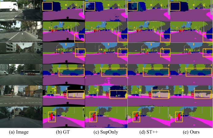
Figure E7: Qualitative results on the Cityscapes val set.(a) and (b) are corresponding to images and Ground Truth(GT), (c) represents the results of supervised baseline(SupOnly), (d) is the results of ST++ [53], and (e) is the results of our framework. Orange rectangles highlight the difference among of them.

Figure E8: Qualitative results on the MoNuSeg test set.(a) and (b) are corresponding to images and Ground Truth(GT), (c) represents the results of supervised baseline(SupOnly), (d) and (e) is the results of CAC [31] and ST++ [53], and (f) is the results of our framework. Green and red present the predictions and ground truth respectively, while yellow indicates their overlap regions.

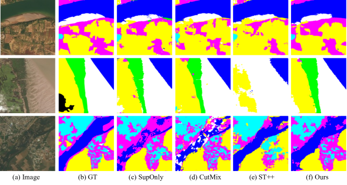
Figure E9: Qualitative results on the DeepGlobe test set.(a) and (b) are corresponding to images and Ground Truth(GT), (c) represents the results of supervised baseline(SupOnly), (d) and (e) is the results of CutMix [56] and ST++ [53], and (f) is the results of our framework. Cyan represents “urban”, yellow represents “agriculture”, magenta represents “rangeland”, green represents “forest”, blue represents “water”, white represents “barren” and black represents “unknown”.

Qualitative results on the Cityscapes val set. On the Cityscapes val set, we present some qualitative results under 1/8 protocol in Figure E7. All of the methods are based on DeepLabv3+ with the ResNet-50. In comparison to the previous state-of-the-art method, our method displays more accurate segmentation results thanks to the proposed progressive learning strategy.

Qualitative results on the MoNuSeg test set. We present some qualitative results under 1/3 protocol in Figure E8 on the MoNuSeg test set. All of the methods are based on DeepLabv3+ with the ResNet-50.

Qualitative results on the DeepGlobe test set. We display some qualitative results under 1/4 protocol in Figure E9 on the DeepGlobe test set. All of the methods are based on DeepLabv3+ with the ResNet-50.

Appendix F Per-class results

In Tables F14 and F15, we present in detail the IOU performance of our results and some other methods for per-class on DeepGlobe and Cityscapes datasets, respectively. It is worth noting that our framework achieves the most significant improvement on the tailed classes (e.g. , ’wall’, ’rider’, ’truck’, ’bus’, and ’train’ ), indicating that our method alleviates the class imbalance issue to a certain extent.

	Urban	Agriculture	Rangeland	Forest	Water	Barren	mIOU(%)
Partition Protocol : 1/16 (28)
SupOnly	74.49	77.23	28.11	61.88	62.57	28.53	55.47
Ours	75.50	75.52	23.96	63.47	75.36	36.36	58.36
Gain	+1.01	-1.71	-4.15	+1.59	+12.79	+7.83	+2.89
Partition Protocol : 1/8 (56)
SupOnly	75.44	82.77	29.21	67.32	67.67	50.73	62.19
Ours	75.47	82.18	32.73	69.22	77.13	54.32	65.17
Gain	+0.03	-0.59	+3.52	+1.90	+9.46	+3.59	+2.98
Partition Protocol : 1/4 (113)
SupOnly	72.56	85.09	33.17	76.99	74.15	58.94	66.82
Ours	77.37	84.80	35.36	76.36	77.18	60.00	68.51
Gain	+4.81	-0.29	+2.19	-0.63	+3.03	+1.06	+1.69
Partition Protocol : Full (454)
SupOnly	76.52	85.13	37.73	75.80	75.99	60.68	68.64
Ours	78.19	86.08	40.23	75.50	78.86	61.16	70.01
Gain	+1.67	+0.95	+2.50	-0.30	+2.87	+0.48	+1.37

Table F14: Results (IoU) of different classes on the DeepGlobe test set under different partition protocols. We use DeepLabv3+ as the segmentation network and ResNet-50 as the backbone. Gain: The mIOU gain of between SupOnly and our approach.

	road	sidewalk	building	wall	fence	pole	light	sign	vegetation	terrain	sky	person	rider	car	truck	bus	train	motorcycle	bicycle	mIOU(%)
Partition Protocol : 1/16 (186)
SupOnly	96.0	73.9	89.4	29.2	41.3	54.9	62.9	70.8	90.6	56.6	92.3	74.2	44.5	91.5	36.7	42.0	23.6	39.8	70.7	62.2
Ours	97.7	82.6	91.2	49.0	55.8	59.7	68.5	77.7	92.0	60.0	94.0	80.2	57.5	94.6	73.1	76.9	68.5	60.7	75.1	74.5
Gain	+1.7	+8.7	+1.8	+19.8	+14.5	+4.8	+5.6	+6.9	+1.4	+3.4	+1.7	+6.0	+13.0	+3.1	+36.4	+34.9	+44.9	+20.9	+4.4	+12.3
Partition Protocol : 1/8 (372)
SupOnly	96.5	77.1	90.7	37.6	51.5	60.1	64.9	74.8	91.5	55.8	93.4	76.6	51.5	93.1	52.0	67.2	48.5	55.5	73.6	69.1
Ours	97.9	83.9	92.3	58.7	60.4	63.5	70.8	79.2	92.3	60.9	94.7	81.9	62.1	95.1	76.1	79.2	71.8	64.8	76.9	77.0
Gain	+1.4	+6.8	+1.6	+21.1	+8.9	+3.4	+5.9	+4.4	+0.8	+5.1	+1.3	+5.3	+10.6	+2.0	+24.1	+12.0	+23.3	+9.3	+3.3	+7.9
Partition Protocol : 1/4 (744)
SupOnly	97.5	81.4	91.2	37.6	55.8	63.4	68.7	77.1	91.6	57.8	93.8	79.1	57.1	93.4	60.7	73.7	55.6	63.0	75.0	72.3
Ours	97.7	83.3	92.8	61.9	63.1	64.9	71.2	79.7	92.5	60.0	94.4	82.8	64.4	95.3	76.8	87.1	78.8	68.7	77.8	78.6
Gain	+0.2	+1.9	+1.6	+24.3	+7.3	+1.5	+2.5	+2.6	+0.9	+2.2	+0.6	+3.7	+7.3	+1.9	+16.1	+13.4	+23.2	+5.7	+2.8	+6.3

Table F15: Results (IoU) of different classes on the Cityscapes val set under different partition protocols. We use DeepLabv3+ as the segmentation network and ResNet-101 as the backbone. Gain: The mIOU gain of between SupOnly and our approach. our framework achieves the most significant improvement on the tailed classes (e.g. , ’wall’, ’rider’, ’truck’, ’bus’, and ’train’ ), indicating that our method alleviates the class imbalance issue to a certain extent.

References

- [1] Nikita Araslanov and Stefan Roth. Self-supervised augmentation consistency for adapting semantic segmentation. In CVPR, pages 15384–15394, June 2021.
- [2] David Berthelot, Nicholas Carlini, Ian Goodfellow, Nicolas Papernot, Avital Oliver, and Colin A Raffel. Mixmatch: A holistic approach to semi-supervised learning. In NeurIPS, volume 32, 2019.
- [3] Kai Chen, Lanqing Hong, Hang Xu, Zhenguo Li, and Dit-Yan Yeung. Multisiam: Self-supervised multi-instance siamese representation learning for autonomous driving. In ICCV, pages 7546–7554, 2021.
- [4] Liang-Chieh Chen, Yukun Zhu, George Papandreou, Florian Schroff, and Hartwig Adam. Encoder-decoder with atrous separable convolution for semantic image segmentation. In ECCV, pages 801–818, 2018.
- [5] Ting Chen, Simon Kornblith, Mohammad Norouzi, and Geoffrey Hinton. A simple framework for contrastive learning of visual representations. In ICML, pages 1597–1607. PMLR, 2020.
- [6] Wuyang Chen, Ziyu Jiang, Zhangyang Wang, Kexin Cui, and Xiaoning Qian. Collaborative global-local networks for memory-efficient segmentation of ultra-high resolution images. In CVPR, pages 8924–8933, 2019.
- [7] Xinlei Chen and Kaiming He. Exploring simple siamese representation learning. In CVPR, pages 15750–15758, 2021.
- [8] Xiaokang Chen, Yuhui Yuan, Gang Zeng, and Jingdong Wang. Semi-supervised semantic segmentation with cross pseudo supervision. In CVPR, pages 2613–2622, 2021.
- [9] Marius Cordts, Mohamed Omran, Sebastian Ramos, Timo Rehfeld, Markus Enzweiler, Rodrigo Benenson, Uwe Franke, Stefan Roth, and Bernt Schiele. The cityscapes dataset for semantic urban scene understanding. In CVPR, pages 3213–3223, 2016.
- [10] Ilke Demir, Krzysztof Koperski, David Lindenbaum, Guan Pang, Jing Huang, Saikat Basu, Forest Hughes, Devis Tuia, and Ramesh Raskar. Deepglobe 2018: A challenge to parse the earth through satellite images. In CVPRW, pages 172–181, 2018.
- [11] Jia Deng, Wei Dong, Richard Socher, Li-Jia Li, Kai Li, and Li Fei-Fei. Imagenet: A large-scale hierarchical image database. In CVPR, pages 248–255. Ieee, 2009.
- [12] Robert Dupre, Jiri Fajtl, Vasileios Argyriou, and Paolo Remagnino. Improving dataset volumes and model accuracy with semi-supervised iterative self-learning. IEEE TIP, 29:4337–4348, 2019.
- [13] Jiashuo Fan, Bin Gao, Huan Jin, and Lihui Jiang. Ucc: Uncertainty guided cross-head co-training for semi-supervised semantic segmentation. In CVPR, pages 9947–9956, 2022.
- [14] Siqi Fan, Fenghua Zhu, Zunlei Feng, Yisheng Lv, Mingli Song, and Fei-Yue Wang. Conservative-progressive collaborative learning for semi-supervised semantic segmentation. IEEE Transactions on Image Processing, pages 1–1, 2023.
- [15] Ian Goodfellow, Jean Pouget-Abadie, Mehdi Mirza, Bing Xu, David Warde-Farley, Sherjil Ozair, Aaron Courville, and Yoshua Bengio. Generative adversarial networks. Communications of the ACM, 63(11):139–144, 2020.
- [16] Yves Grandvalet and Yoshua Bengio. Semi-supervised learning by entropy minimization. In NeurIPS, volume 17, 2004.
- [17] Dayan Guan, Jiaxing Huang, Aoran Xiao, and Shijian Lu. Unbiased subclass regularization for semi-supervised semantic segmentation. In CVPR, pages 9968–9978, 2022.
- [18] Yuying Hao, Yi Liu, Zewu Wu, Lin Han, Yizhou Chen, Guowei Chen, Lutao Chu, Shiyu Tang, Zhiliang Yu, Zeyu Chen, et al. Edgeflow: Achieving practical interactive segmentation with edge-guided flow. In CVPR, pages 1551–1560, 2021.
- [19] Kaiming He, Haoqi Fan, Yuxin Wu, Saining Xie, and Ross Girshick. Momentum contrast for unsupervised visual representation learning. In CVPR, pages 9729–9738, 2020.
- [20] Kaiming He, Xiangyu Zhang, Shaoqing Ren, and Jian Sun. Deep residual learning for image recognition. In CVPR, pages 770–778, 2016.
- [21] Ruifei He, Jihan Yang, and Xiaojuan Qi. Re-distributing biased pseudo labels for semi-supervised semantic segmentation: A baseline investigation. In ICCV, 2021.
- [22] Jinyong Hou, Xuejie Ding, and Jeremiah D Deng. Semi-supervised semantic segmentation of vessel images using leaking perturbations. In WACV, pages 2625–2634, 2022.
- [23] Hanzhe Hu, Fangyun Wei, Han Hu, Qiwei Ye, Jinshi Cui, and Liwei Wang. Semi-supervised semantic segmentation via adaptive equalization learning. In NeurIPS, volume 34, pages 22106–22118, 2021.
- [24] Wei Chih Hung, Yi Hsuan Tsai, Yan Ting Liou, Yen-Yu Lin, and Ming Hsuan Yang. Adversarial learning for semi-supervised semantic segmentation. In BMVC, 2018.
- [25] Sergey Ioffe and Christian Szegedy. Batch normalization: Accelerating deep network training by reducing internal covariate shift. In ICML, pages 448–456. PMLR, 2015.
- [26] Ashish Jaiswal, Ashwin Ramesh Babu, Mohammad Zaki Zadeh, Debapriya Banerjee, and Fillia Makedon. A survey on contrastive self-supervised learning. Technologies, 9(1):2, 2020.
- [27] Zhanghan Ke, Di Qiu, Kaican Li, Qiong Yan, and Rynson WH Lau. Guided collaborative training for pixel-wise semi-supervised learning. In ECCV, pages 429–445. Springer, 2020.
- [28] Minsu Ko, Eunju Cha, Sungjoo Suh, Huijin Lee, Jae-Joon Han, Jinwoo Shin, and Bohyung Han. Self-supervised dense consistency regularization for image-to-image translation. In Proceedings of the IEEE/CVF Conference on Computer Vision and Pattern Recognition, pages 18301–18310, 2022.
- [29] Neeraj Kumar, Ruchika Verma, Deepak Anand, Yanning Zhou, Omer Fahri Onder, Efstratios Tsougenis, Hao Chen, Pheng-Ann Heng, Jiahui Li, Zhiqiang Hu, et al. A multi-organ nucleus segmentation challenge. IEEE transactions on medical imaging, 39(5):1380–1391, 2019.
- [30] Donghyeon Kwon and Suha Kwak. Semi-supervised semantic segmentation with error localization network. In CVPR, pages 9957–9967, 2022.
- [31] Xin Lai, Zhuotao Tian, Li Jiang, Shu Liu, Hengshuang Zhao, Liwei Wang, and Jiaya Jia. Semi-supervised semantic segmentation with directional context-aware consistency. In CVPR, pages 1205–1214, 2021.
- [32] Jerome Y Lettvin et al. On seeing sidelong. The Sciences, 16(4):10–20, 1976.
- [33] Huan Ling, Jun Gao, Amlan Kar, Wenzheng Chen, and Sanja Fidler. Fast interactive object annotation with curve-gcn. In CVPR, pages 5257–5266, 2019.
- [34] Yuyuan Liu, Yu Tian, Yuanhong Chen, Fengbei Liu, Vasileios Belagiannis, and Gustavo Carneiro. Perturbed and strict mean teachers for semi-supervised semantic segmentation. In CVPR, pages 4258–4267, 2022.
- [35] Juhong Min, Yucheng Zhao, Chong Luo, and Minsu Cho. Peripheral vision transformer. In NeurIPS, 2022.
- [36] Sudhanshu Mittal, Maxim Tatarchenko, and Thomas Brox. Semi-supervised semantic segmentation with high-and low-level consistency. IEEE TPAMI, 43(4):1369–1379, 2019.
- [37] Takeru Miyato, Shin-ichi Maeda, Masanori Koyama, and Shin Ishii. Virtual adversarial training: a regularization method for supervised and semi-supervised learning. IEEE TPAMI, 41(8):1979–1993, 2018.
- [38] Viktor Olsson, Wilhelm Tranheden, Juliano Pinto, and Lennart Svensson. Classmix: Segmentation-based data augmentation for semi-supervised learning. In WACV, pages 1369–1378, 2021.
- [39] Aaron van den Oord, Yazhe Li, and Oriol Vinyals. Representation learning with contrastive predictive coding. arXiv preprint arXiv:1807.03748, 2018.
- [40] Yassine Ouali, Céline Hudelot, and Myriam Tami. Semi-supervised semantic segmentation with cross-consistency training. In CVPR, pages 12674–12684, 2020.
- [41] Olaf Ronneberger, Philipp Fischer, and Thomas Brox. U-net: Convolutional networks for biomedical image segmentation. In International Conference on Medical image computing and computer-assisted intervention, pages 234–241. Springer, 2015.
- [42] Connor Shorten and Taghi M Khoshgoftaar. A survey on image data augmentation for deep learning. Journal of big data, 6(1):1–48, 2019.
- [43] Abhinav Shrivastava, Abhinav Gupta, and Ross Girshick. Training region-based object detectors with online hard example mining. In CVPR, pages 761–769, 2016.
- [44] Kihyuk Sohn, David Berthelot, Nicholas Carlini, Zizhao Zhang, Han Zhang, Colin A Raffel, Ekin Dogus Cubuk, Alexey Kurakin, and Chun-Liang Li. Fixmatch: Simplifying semi-supervised learning with consistency and confidence. In NeurIPS, volume 33, pages 596–608, 2020.
- [45] Nasim Souly, Concetto Spampinato, and Mubarak Shah. Semi supervised semantic segmentation using generative adversarial network. In ICCV, pages 5688–5696, 2017.
- [46] Xian Sun, Aijun Shi, Hai Huang, and Helmut Mayer. Bas4net: Boundary-aware semi-supervised semantic segmentation network for very high resolution remote sensing images. IEEE Journal of Selected Topics in Applied Earth Observations and Remote Sensing, 13:5398–5413, 2020.
- [47] Xin-Yi Tong, Gui-Song Xia, Qikai Lu, Huanfeng Shen, Shengyang Li, Shucheng You, and Liangpei Zhang. Land-cover classification with high-resolution remote sensing images using transferable deep models. Remote Sensing of Environment, 237:111322, 2020.
- [48] Yuchao Wang, Haochen Wang, Yujun Shen, Jingjing Fei, Wei Li, Guoqiang Jin, Liwei Wu, Rui Zhao, and Xinyi Le. Semi-supervised semantic segmentation using unreliable pseudo-labels. In CVPR, pages 4248–4257, 2022.
- [49] Huisi Wu, Zhaoze Wang, Youyi Song, Lin Yang, and Jing Qin. Cross-patch dense contrastive learning for semi-supervised segmentation of cellular nuclei in histopathologic images. In CVPR, pages 11666–11675, 2022.
- [50] Hui Xiao, Dong Li, Hao Xu, Shuibo Fu, Diqun Yan, Kangkang Song, and Chengbin Peng. Semi-supervised semantic segmentation with cross teacher training. Neurocomputing, 508:36–46, 2022.
- [51] Hai-Ming Xu, Lingqiao Liu, Qiuchen Bian, and Zhen Yang. Semi-supervised semantic segmentation with prototype-based consistency regularization. In NeurIPS, 2022.
- [52] Lihe Yang, Lei Qi, Litong Feng, Wayne Zhang, and Yinghuan Shi. Revisiting weak-to-strong consistency in semi-supervised semantic segmentation. In CVPR, 2023.
- [53] Lihe Yang, Wei Zhuo, Lei Qi, Yinghuan Shi, and Yang Gao. St++: Make self-training work better for semi-supervised semantic segmentation. In CVPR, pages 4268–4277, 2022.
- [54] Mang Ye, Xu Zhang, Pong C Yuen, and Shih-Fu Chang. Unsupervised embedding learning via invariant and spreading instance feature. In CVPR, pages 6210–6219, 2019.
- [55] Jianlong Yuan, Yifan Liu, Chunhua Shen, Zhibin Wang, and Hao Li. A simple baseline for semi-supervised semantic segmentation with strong data augmentation. In ICCV, pages 8229–8238, 2021.
- [56] Sangdoo Yun, Dongyoon Han, Seong Joon Oh, Sanghyuk Chun, Junsuk Choe, and Youngjoon Yoo. Cutmix: Regularization strategy to train strong classifiers with localizable features. In ICCV, pages 6023–6032, 2019.
- [57] Hengshuang Zhao, Jianping Shi, Xiaojuan Qi, Xiaogang Wang, and Jiaya Jia. Pyramid scene parsing network. In CVPR, pages 2881–2890, 2017.
- [58] Yuanyi Zhong, Bodi Yuan, Hong Wu, Zhiqiang Yuan, Jian Peng, and Yu-Xiong Wang. Pixel contrastive-consistent semi-supervised semantic segmentation. In ICCV, pages 7273–7282, 2021.
- [59] Barret Zoph, Golnaz Ghiasi, Tsung-Yi Lin, Yin Cui, Hanxiao Liu, Ekin Dogus Cubuk, and Quoc Le. Rethinking pre-training and self-training. In NeurIPS, volume 33, pages 3833–3845, 2020.