Data-Driven Network Neuroscience: On Data Collection and Benchmark

Abstract

This paper presents a comprehensive and quality collection of functional human brain network data for potential research in the intersection of neuroscience, machine learning, and graph analytics. Anatomical and functional MRI images have been used to understand the functional connectivity of the human brain and are particularly important in identifying underlying neurodegenerative conditions such as Alzheimer’s, Parkinson’s, and Autism. Recently, the study of the brain in the form of brain networks using machine learning and graph analytics has become increasingly popular, especially to predict the early onset of these conditions. A brain network, represented as a graph, retains rich structural and positional information that traditional examination methods are unable to capture. However, the lack of publicly accessible brain network data prevents researchers from data-driven explorations. One of the main difficulties lies in the complicated domain-specific preprocessing steps and the exhaustive computation required to convert the data from MRI images into brain networks. We bridge this gap by collecting a large amount of MRI images from public databases and a private source, working with domain experts to make sensible design choices, and preprocessing the MRI images to produce a collection of brain network datasets. The datasets originate from 6 different sources, cover 4 brain conditions, and consist of a total of 2,702 subjects. We test our graph datasets on 12 machine learning models to provide baselines and validate the data quality on a recent graph analysis model. To lower the barrier to entry and promote the research in this interdisciplinary field, we release our brain network data and complete preprocessing details including codes at https://doi.org/10.17608/k6.auckland.21397377 and https://github.com/brainnetuoa/data_driven_network_neuroscience.

1 Introduction

Neuroscience unveils the principles and mechanisms underlying complex brain functions on normal subjects and subjects with neurological, psychiatric, and/or neurodevelopmental conditions. Recent years have witnessed an expansion in the size, scope and complexity of human neural data acquisition. Such an expansion joined with a rapid progress in machine learning and graph analytics has drawn a growing attention in network neuroscience – the neuroscience that comprehends the structure/function of the human brain using graphs (called brain networks) [14]. Each neuron/brain region can be modelled as a node and the interconnectivity between two neurons/brain regions as an edge. Brain networks capture rich structural and functional information that traditional manual examinations fail to capture: communications associated with spontaneous or task-evoked brain activities, dynamic patterns of neural signalling, interactions/disconnections associated with certain diseases, etc. [7].

Network neuroscience leverages on graph-based machine learning for clinically important applications. For example, a community in brain networks could represent areas of co-activation that could be weakened on brains with neurodegenerative conditions [34]. Graph classification [19] can help differentiate subjects with neurological diseases from healthy ones. Graph ordinal regression [38] can identify subjects with different stages of neurological diseases based on the severity. Nonetheless, the potential of graph-based machine learning in clinical applications is hindered by the scarcity of available brain network datasets in this important interdisciplinary field.

In this study, we focus on functional magnetic resonance imaging (fMRI), which monitors changes in the blood flow, i.e., blood-oxygen-level-dependent (BOLD) signals to capture functional activities [24]. The conversion of fMRI scans to brain networks has two stages, preprocessing and parcellation, both requiring intensive domain inputs. Specifically, to ensure the image quality for subsequent tasks, the preprocessing of raw MRI images needs proper quality control over a number of steps, including motion correction, realigning, field unwarping, normalization, bias field correction, and brain extraction. Different preprocessing choices lead to a large variation in the output images. Parcellation translates the preprocessed MRI images to regions-of-interest (ROIs) as nodes and the co-activation between ROIs as weighted edges. Each generated brain network contains i) a weighted adjacency matrix that characterizes the connectivity between ROIs and ii) a feature matrix that captures the attributes of ROIs in terms of the aggregated BOLD signals. Choosing a different brain atlas/scheme for parcellation leads to a different brain network. Existing study typically selects a single parcellation scheme to generate a fixed set of nodes for all subjects in the study, while the effect of different choices of group-wise data-driven parcellation schemes remains largely unexplored.

The above conversion poses a high barrier to entry the research on brain networks, limiting the development of data-driven network neuroscience. Specifically, domain knowledge in neuroimage preprocessing is required to select and guide the proper pipeline and tools used, image processing and graph extraction lead to high computational costs, and large-scale imaging studies require a complex setup with multi-site, multi-scanner, and multiple acquisition protocols. This paper aims to bridge the gap by making more brain network data available to the public. We believe that releasing this brain network collection will promote research in the interdisciplinary field of network neuroscience, machine learning, and graph analytics, and advance graph-based and clinical studies such as the detection of neurodegenerative conditions. Our main contributions are highlighted below.

1. We release a large resting-state functional brain network collection to the public. The collection was originated from 6 raw rs-fMRI image sources with 5 well recognized ones in neuroscience and one new data source, covering 3 neurodegenerative and one brain injury conditions, i.e., Autism, Alzheimer, Parkinson, and mTBI. The collection consists of ABIDE (N=1025), ADNI (N=1327), PPMI (N=209), Mātai (N=60) and two other sources totalling to 2,702 subjects.

2. We test the datasets on one recent graph analysis model [34], 6 conventional machine learning (ML) models, as well as 6 representative graph ML models. The experimental results demonstrate that the quality of our datasets is not compromised by the conversion process and can serve as a domain benchmark for subsequent research.

2 Related Work

Data Collection. Preprocessed Connectomes Project (PCP) [17] is an initiative to preprocess part of the raw MRI images in the International Neuroimaging Data-sharing Initiative (INDI) database and make the preprocessed neuroimages publicly available. Within PCP, one relevant dataset that has gone through functional preprocessing pipelines is the ABIDE dataset on Autism. Note that the pipeline used for preprocessing ABIDE was proposed in 2012 [9] while the state-of-the-art functional preprocessing pipeline is fMRIPrep [20] which introduces less uncontrolled spatial smoothness [20] compared to other preprocessing tools. Some work converts preprocessed neuroimages to brain network datasets which, however, are predominately binarized, i.e., the edge weight can take only two values $0$ or $1$. For example, in [34], the ABIDE dataset was converted to binarized brain networks. In [42, 1], around 80 samples for Attention Deficit Hyperactivity Disorder (ADHD) were released in three datasets KKI, OHSU, and Peking_1 in the form of binarized brain networks. There still lacks a large collection of quality brain network datasets available to the public. Our collection uses fMRIPrep on data from 6 sources (see Section 3 for details) on 4 clinical conditions of interest under different parcellation schemes and wraps the whole conversion process from raw MRI images to brain networks in a holistic manner. We release the codes of the entire processing pipeline and keep future efforts in refining the pipeline and/or enriching the collection open.

Benchmark. Network neuroscience that uses machine learning and graph analytics has attracted an increasing attention [23]. Along this line of research, most recent studies [10, 46, 37, 30, 34] apply machine learning models to perform connectivity analysis on the ABIDE dataset with the generated brain networks. In our benchmark, we tested our datasets on one recent graph analysis model [34], 6 conventional ML models and 6 representative graph ML models: the quality of our datasets is not compromised by the conversion process and can serve as baselines for this line of research.

3 Dataset Sources: Raw Neuroimages

This section describes our selected sources of raw neuroimages and their selection and acquisition settings. Table 1 summarizes our datasets and the generated brain networks. This paper focuses on resting-state functional connectivity of the brain using rs-fMRI, a potent method for detecting neurodegenerative conditions [24], leaving alternative modalities for future exploration. To achieve quality image preprocessing, each rs-fMRI image needs a structural T1-weighted (T1w) image that was acquired from the same subject in the same scan session. T1w image provides structural details which allow brain mask extraction, image alignment and BOLD time series normalization. Other pipelines such as DPARSF [54] have the same requirement.

Table 1: Statistics of our datasets and the generated resting-state functional brain networks. Each subject has a graph (brain connectivity network) generated under each Parcellation Method (PM) of AAL, HarvardOxford (HO), Schaefer, k-means and Ward Clustering (see Table 2 for details). The number of nodes in a graph generated under a PM is the number of ROIs of the PM. We call an edge non-zero if its weight has absolute value $>10^{-2}$. The number of non-zero edges varies under different parcellations. The number of node features is the length of the BOLD signals.

		# of Graphs	# of	Avg # Non-Zero Edges under PM (# of Nodes)					Avg #
Dataset	Condition	(# of Subjects)	Classes	AAL	HO	Schaefer	$k$-means	Ward	of Node
				(116)	(48)	(100)	(100)	(100)	Features
ABIDE	Autism	1025	2	6402	1112	4811	4698	4729	201
ADNI	Alzheimer	1327	6	6447	1112	4824	4734	4715	344
PPMI	Parkinson	209	4	6512	1122	4866	4795	4684	198
Mātai	mTBI	60	2	6433	1112	4832	4750	4731	198
TaoWu	Parkinson	40	2	6481	1116	4846	4724	4766	239
Neurocon	Parkinson	41	2	6455	1114	4830	4677	4779	137

Autism Brain Imaging Data Exchange (ABIDE) The ABIDE initiative aggregated functional brain imaging data collected from laboratories around the world to support the research on Autism Spectrum Disorder (ASD). ASD has stereotyped behaviors such as irritability, hyperactivity, depression, and anxiety. Subjects are classified into typical controls and those suffering from ASD.

Alzheimer’s Disease Neuroimaging Initiative (ADNI) ADNI [4, 3, 52] is a longitudinal multisite study for the early detection and tracking of Alzheimer’s Disease (AD). AD is a progressive neurologic disorder that causes the brain to shrink and brain cells to die and is the most common cause of dementia that affects a person’s ability to function independently. ADNI data used in this study were obtained from the ADNI database (adni.loni.usc.edu) which was launched in 2003 as a public-private partnership, led by Principal Investigator Michael W. Weiner, MD. The primary goal of ADNI has been to test whether serial MRI, positron emission tomography (PET), other biological markers, and clinical and neuropsychological assessment can be combined to measure the progression of mild cognitive impairment (MCI) and early Alzheimer’s disease (AD). Subjects are from 6 different stages of AD: cognitive normal (CN), significant memory concern (SMC), mild cognitive impairment (MCI), early MCI (EMCI), late MCI (LMCI), and Alzheimer’s disease (AD) [8].

Parkinson’s Progression Markers Initiative (PPMI) PPMI aims to identify biological markers of Parkinson’s risk, onset and progression. Parkinson’s disease is a progressive nervous system disorder that mainly affects movement [41]. The study is ongoing and contains multimodal, multi-site MRI images similar to ADNI. The PPMI dataset contains subjects from 4 classes: normal control, scans without evidence of dopaminergic deficit (SWEDD), prodromal, and Parkinson’s disease (PD).

Mātai Mātai is a longitudinal single site, single scanner study designed for detecting subtle changes in the brain due to a season of playing contact sports. This new dataset consists of the brain networks preprocessed from the data collected from Gisborne-Tairāwhiti area, New Zealand, with 35 contact sport players imaged at pre-season (N=35) and post-season (N=25) with subtle brain changes confirmed using diffusion imaging study due to playing contact sports. Note that this dataset does not release raw data nor metadata and has been preprocessed so that no ancestral history is able to be extracted.

TaoWu and Neurocon TaoWu and Neurocon datasets are released by ICI [6] and are two of the earliest image datasets released for Parkinson’s. The datasets consist of age-matched subjects captured using a single machine and on a single site. We include these two datasets in our collection as they could be used in studies that aim to minimize or contrast the variability introduced from different image acquisition settings. It includes normal controls and patients labelled with PD. Neurocon and Taowu label patients with a diagnosis of PD who have been under treatment (most under levodopa) as PD. PPMI’s PD definition involves patients with a diagnosis of PD for two years or less and who are not taking PD medications. Under these definitions, Neurocon and Taowu are more similar when compared to PPMI. It is worth noting that while these two have similar scanning protocols, they used different scanners (with Taowu being higher in resolution). In [6], the authors compared these scans and argued that they can be treated similarly. We believe there could be more such explorations with the data available, which is one of the main reasons why we want to release this collection.

4 From MRI Images to Brain Networks: Design Choices

We adopt the common functional processing pipeline in network neuroscience [21] to convert raw MRI images (rs-fMRI and T1w) into brain networks, as depicted in Figure 1. Under this general pipeline, a number of choices need to be made in data selection, data formats, neuro-image preprocessing tools, parcellation schemes, network edge formation, etc. We worked closely with our domain experts to ensure that our design choices are sensible and state-of-the-art. Specifically, Step A collects raw MRI images based on the selection criteria (Section 4.1). Step B converts the images into BIDS format (Section 4.2). Step C preprocesses the images using fMRIPrep (Section 4.3). Step D parcellates the preprocessed data into different ROIs (Section 4.4). Steps E-F extract the connectivity matrix and the feature matrix and form the brain network (Section 4.5). Domain experts have guided our preprocessing by providing advice/feedback on i) the selection of images from the data sources, ii) the choices of using the state-of-the-art fMRIPrep pipeline, iii) parcellation strategies, iv) quality check of fMRIPrep outputs, and v) the selection of confounds.

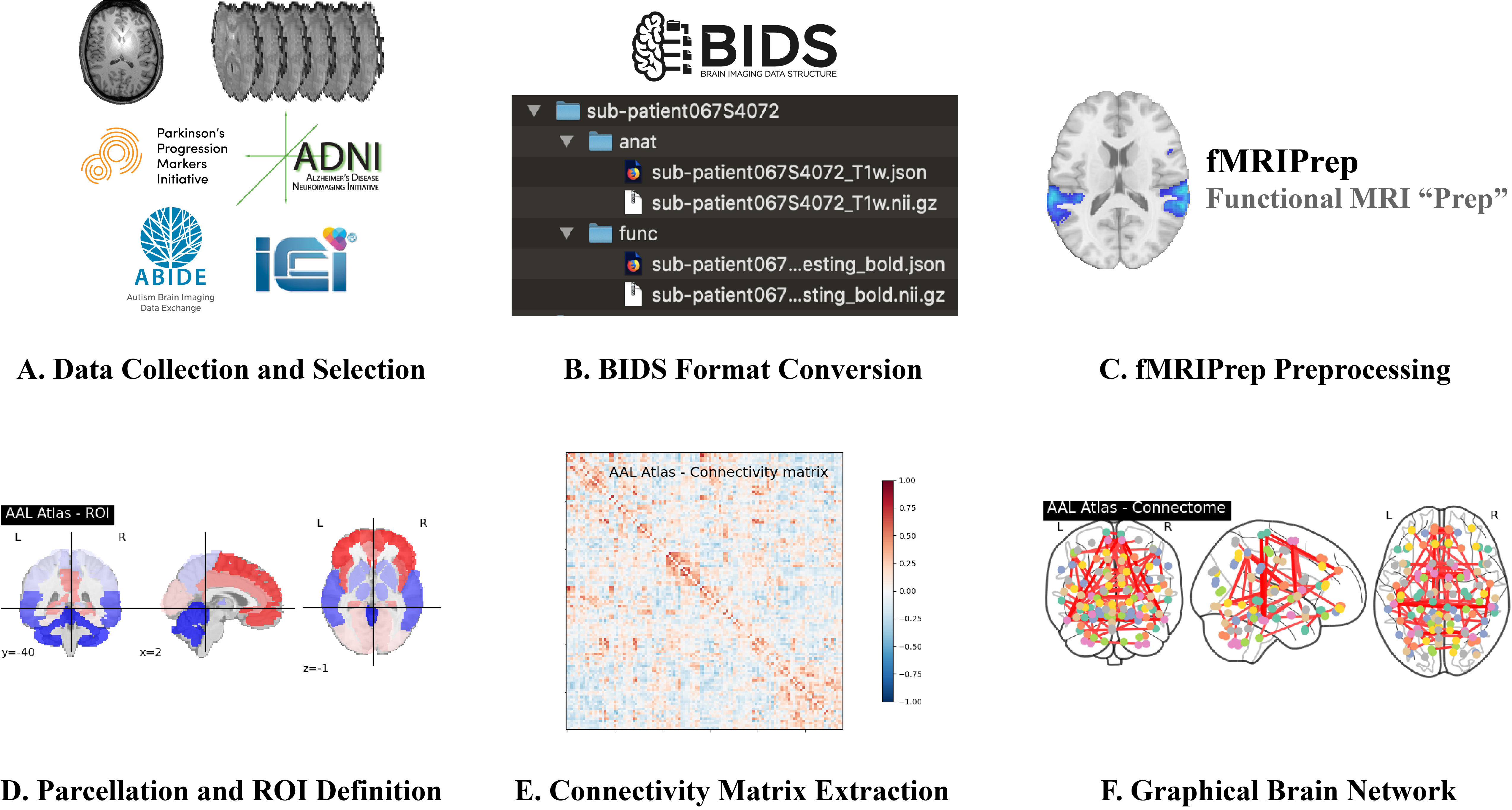
Figure 1: Brain Network Construction Pipeline

4.1 Data Collection and Selection Criteria

Our data sources involve multi-site, muti-scanner images. Thus, the inclusion criteria of our data collection is based on the availability, validity, and quality of the MRI images of our required types.

For ABIDE, TaoWu, and Neurocon, the original source images were already collated with 1 raw rs-fMRI image paired with 1 T1w image for each subject. We included all subjects provided by these data sources except for those that had quality issues. A subject has quality issues if it has an incomplete image (i.e., not containing the full brain) and/or damaged data (i.e., with error reported by any subsequent preprocessing steps). Available metadata of each subject from the source is included in our collection, such as age and gender. The gender distributions of our datasets closely match those of the original data sources. The only exception is ADNI: our released data contains 0.6% more females than the original ADNI data.

For longitudinal study data sources ADNI, PPMI, and Mātai, it is possible that some subjects have had multiple scans over the course of several years. Depending on the scanning protocol for the study, different types of images were taken at various times (e.g., baseline, 1 year follow-up, 2 year follow-up, etc.). The baseline study (the first scan) is usually the most comprehensive one that would cover a wide range of modalities. Thus, as suggested by our domain experts, we consider the baseline study which is likely to be the set of scans with both an rs-fMRI image and a T1w image taken on the same date. In the case that multiple rs-fMRI and T1w scans exist, we selected the first available one.

ABIDE, ADNI, and PPMI are multi-site neuroimaging sources. We chose not to apply data harmonization techniques to these datasets in our preprocessing due to the following reasons. (1) For fMRI connectivity, there is no well-grounded harmonization method for benchmark. (2) Even though no fMRI connectivity harmonization was applied, [43] has shown that fMRI connectivity still has some good repeatability. (3) The site and scanner information are available and researchers have the flexibility of performing harmonization based on our data collection for further analysis.

For validity, we examined each image manually to make sure the images conformed to their labels in the database and did not have obvious data format issues for preprocessing. We had to check this manually because the image databases often had inconsistent labeling.

4.2 BIDS Conversion

Raw MRI images are typically in the Digital Imaging and Communications in Medicine (DICOM) format. DICOM images are then converted to the Neuroimaging Informatics Technology Initiative (NIfTI) format using dcm2niix [36], which includes a JSON file that details various imaging parameters such as scanner model, magnetic field strength, flip angle, slice timing, echo time and repetition time. The NIfTI and JSON files are then organized into a folder hierarchy with a precise naming convention known as Brain Imaging Data Structure (BIDS) [27]. After conversion, BIDS formatted data can be applied to preprocessing pipelines in a highly reproducible and transparent manner.

4.3 fMRIPrep Preprocessing

BIDS compliant datasets are then preprocessed using fMRIPrep [20], a state-of-the-art tool for preprocessing fMRI. fMRIPrep performs basic processing steps (coregistration, normalization, noise component extraction, skull stripping, etc.) and uses a combination of tools from well-known software packages, including FMRIB Software Library (FSL) [31], Analysis of Functional NeuroImages (AFNI) [16], Advanced Normalization Tools (ANT) [5] and FreeSurfer [22]. This pipeline was designed to use the best software implementation for each step of preprocessing. fMRIPrep can be installed via container technologies such as docker or singularity. fMRIPrep automates the pipeline by using the scanner outputs from the images (e.g., slice timing correction parameters are taken automatically from the scanner outputs of the original image data). Therefore, the user does not need to specify these parameters manually. fMRIPrep can be configured to include or exclude specific workflow steps, such as ignoring slice timing. We followed the default automatic fMRIPrep workflow with surface reconstruction enabled. No further modifications to the settings were made as the default workflow met our expectations for a functional preprocessing pipeline. As part of our validation process of fMRIPrep, we have passed the preprocessed images over to our MRI imaging experts: they have carefully examined the outputs to ensure the data quality. fMRIPrep outputs conform to the BIDS Derivatives specification for compatibility and include the preprocessed BOLD images and the confounds file, which records fluctuations during MRI data acquisition, also known as nuisance regressors. fMRIPrep is computationally expensive. In our case, one run on one subject of fMRIPrep using 8 threads on an Intel(R) Core(TM) i9-10940X CPU@3.30GHz took on average 4-5 hours.

4.4 Parcellation Strategies

Parcellation defines regions in the brain known as region-of-interest (ROI). The parcellation step takes in the two outputs from fMRIPrep for each subject to generate the parcellations: the preprocessed BOLD image and the confounds file. We adopted the standard 9 parameters (9P) confounds setting widely used in functional connectivity studies [25, 26] for denoising: white matter, cerebrospinal fluid, global signal, and the 6 rigid-body motion parameters for rotation and translations at $x$, $y$ and $z$ axes. To parcellate the brain, we selected a list (Table 2) of Parcellation Methods (PMs) that cover both atlas-based and clustering-based PMs frequently used in the domain.

Table 2: Parcellation Methods

Name	# ROIs	Generation Method
AAL [49]	116	Delineated with respect to anatomical landmarks by following the sulci course in the brain.
HarvardOxford (HO) [40]	48	Created by subdividing neocortex by topographic criteria into 48 parcellation units corresponding to the principal cerebral gyri.
Schaefer [47]	100	Using gradient-weighted Markov Random Fields (gwMRF) to automatically group similar fMRI regions.
$k$-means Clustering [39, 2]	100	Top-down clustering algorithm that partitions voxels into non-overlapping predefined number of regions.
Ward Clustering [51, 2]	100	Bottom-up hierarchical clustering algorithm that agglomerates together voxels progressively into regions.

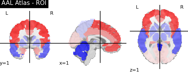
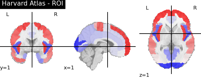
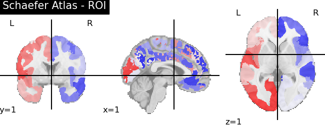
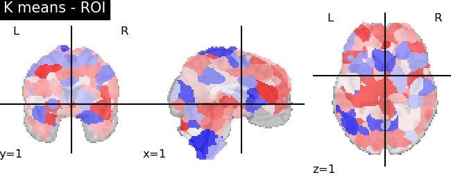
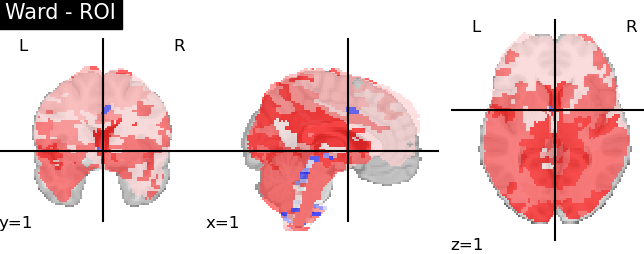
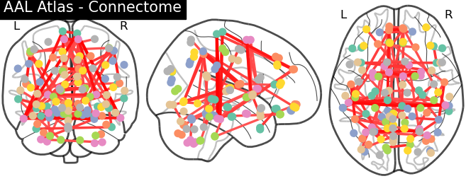
Figure 2: Extracted ROIs and Glass Brain Connectome (right bottom corner)

Brain regions partitioned through predefined regions are atlas-based PMs. We selected the most commonly used atlas-based PMs, AAL, HarvardOxford (HO), and Schaefer, that are generated using different strategies and brain features. Clustering-based parcellations partition the brain by computing the similarity in the BOLD signals between voxels and performing clustering on the voxels based on the similarities. Each subject directly generates its own set of ROIs. $k$-means and Ward clustering are the two methods used in the domain. We included them and set the number of ROIs as 100, which is close to the predefined value in atlas-based PMs. Our datasheet in the Supplementary details the file format and output files. Figure 2 shows examples of the ROIs extracted by these methods.

4.5 Brain Network Extraction

The BOLD signals from parcellated ROIs are used to compute the connectivity matrix of the brain network. The matrix captures functional relationships between parcellated regions and reflects their co-activations. Connectivity matrix is extracted using a built-in function of nilearn [2] called ConnectivityMeasures [55]. It takes 2 inputs, BOLD signals of the brain regions and the connectivity metric (e.g., correlation). The former is obtained by averaging the BOLD signals of all the voxels lying in the same ROI. Figure 1E shows an example of a connectivity matrix. Among existing connectivity measures (correlation, covariance, partial correlation, etc.), correlation is used by a majority of graph-based neuroscience research [34, 37, 44]. Thus, in our released collection, we select correlation as the connectivity measure and make the fully weighted matrices available without performing any thresholding on the correlation values. For the practitioners who are interested in alternative measures, we have uploaded preprocessed images (excluding the Mātai dataset) and our matrix generation code as part of our collection, which enables the researchers to generate their own matrices based on their desired measure. The datasheet in our Supplementary details our outputs and file formats. The connectivity matrix can be represented equivalently as a glass brain connectome. An example connectome plot on the AAL atlas is shown in the right bottom corner of Figure 2. The connectome plot shows top 1% of brain functional connectivities for visualization.

The brain network constructed by this pipeline has the set of ROIs as nodes and their co-activations (measured as Correlation) as edges. Each brain network is represented by a weighted adjacency matrix and a feature matrix. The former is the connectivity matrix extracted and the latter stores the BOLD signals of ROIs. Note that we include the BOLD signals as node feature matrices in our data release for data completeness: some analytical methods on brain networks may want to utilize such information directly or further extract features from them.

5 Data Quality Assessment and Baseline Comparisons

To assess if the graph representation maintains the data quality from neuroimages, we test our brain network data collection on two tasks, graph classification and graph ordinal regression. The aim of graph classification is to distinguish patients from healthy subjects for datasets with two classes (ABIDE, Mātai, TaoWu, and Neurocon); and to distinguish subjects among different disease stages and healthy groups by treating each class independently when it comes to multi-class datasets (ADNI and PPMI). In contrast, graph ordinal regression is only applied to multi-class datasets by differentiating stages based on the disease severity.

For classification, we test on both conventional ML models typically used in neuroscience and representative graph ML models. For conventional models, we follow the common practice in the domain [10, 30] to vectorize the input connectivity matrices by flattening them. For ordinal regression, we test on the classic logistic ordinal regression model. To further validate the quality of our data, we also test on a recent graph analysis model on functional networks for classification [34]. Finally, we also include a sensitivity study on the number of ROIs and the training set size. All these models only utilize the connectivity matrices for assessing the quality of our brain network construction. The data is split to 8:1:1 for training, validation, and testing with 10-fold cross-validation performed.

5.1 Results on Classification

We select 6 conventional machine learning models for this study: Logistic Regression (LR), Gaussian Naive Bayes (NB), Support Vector Machine Classifier (SVC), $k$-Nearest Neighbours (kNN), Random Forest (RF), and Multi-Layer Perceptron (MLP) [29]. We used the implementation from the scikit-learn library [45, 11] with Grid Search for model selection. We also select 6 typical graph-based machine learning models, including GCN [33], GraphSAGE [28], GIN [53], GAT [50], GatedGCN [12], and BrainNetCNN [32]. The implementations mainly follow those in [18]. To compare the effectiveness of brain networks with that of BOLD signals in disease classification, we test on two methods based on BOLD signals: GRU [15] and 1D-CNN [35].

Table 3: Classification accuracy (mean$\pm$standard deviation) on conventional ML methods. The best result at each parcellation is highlighted in bold. The best result in each dataset is underlined.

ABIDE						ADNI
	AAL	HO	Schaefer	$k$-means	Ward	AAL	HO	Schaefer	$k$-means	Ward
LR	63.8$\pm$3.0	63.6$\pm$4.2	64.8$\pm$3.7	48.4$\pm$4.4	51.1$\pm$5.8	64.1$\pm$1.8	61.9$\pm$2.1	62.0$\pm$4.2	58.6$\pm$2.6	60.4$\pm$0.8
NB	60.4$\pm$5.5	59.2$\pm$5.4	61.6$\pm$3.6	51.6$\pm$3.7	54.2$\pm$5.0	53.6$\pm$4.4	52.7$\pm$6.7	48.9$\pm$3.3	32.5$\pm$3.6	55.0$\pm$2.6
SVC	65.7$\pm$3.3	62.9$\pm$3.6	64.4$\pm$5.1	49.3$\pm$4.1	53.2$\pm$4.9	63.4$\pm$1.9	66.2$\pm$2.9	61.5$\pm$5.0	61.8$\pm$0.3	61.8$\pm$0.3
kNN	58.1$\pm$5.3	56.1$\pm$4.5	59.7$\pm$3.5	50.7$\pm$2.9	49.3$\pm$2.3	60.6$\pm$2.1	62.9$\pm$3.8	63.1$\pm$2.4	31.4$\pm$22.9	59.5$\pm$3.9
RF	62.4$\pm$2.8	60.5$\pm$3.1	62.6$\pm$2.6	49.5$\pm$5.4	51.3$\pm$2.9	61.9$\pm$2.1	61.7$\pm$2.8	62.1$\pm$1.8	61.5$\pm$0.4	61.6$\pm$0.5
MLP	54.4$\pm$1.2	62.2$\pm$4.4	49.6$\pm$4.4	63.6$\pm$3.9	51.7$\pm$6.3	62.4$\pm$1.8	62.9$\pm$2.2	46.7$\pm$5.3	61.7$\pm$0.2	48.6$\pm$5.9
PPMI						Mātai
	AAL	HO	Schaefer	$k$-means	Ward	AAL	HO	Schaefer	$k$-means	Ward
LR	56.0$\pm$7.8	56.0$\pm$9.2	56.5$\pm$6.8	60.3$\pm$7.4	60.3$\pm$8.8	66.7$\pm$21.1	58.3$\pm$13.4	60.0$\pm$20.0	55.0$\pm$ 18.3	58.3$\pm$20.1
NB	58.4$\pm$5.2	52.6$\pm$8.6	57.5$\pm$7.6	58.4$\pm$5.7	62.2$\pm$7.4	68.3$\pm$22.9	45.0$\pm$21.2	56.7$\pm$18.6	55.0$\pm$15.0	53.3$\pm$18.0
SVC	64.1$\pm$5.7	63.6$\pm$6.4	63.2$\pm$8.6	60.8$\pm$7.5	60.8$\pm$8.9	65.0$\pm$20.3	58.3$\pm$13.4	56.7$\pm$17.0	58.3$\pm$17.1	58.3$\pm$17.1
kNN	51.2$\pm$9.1	55.5$\pm$7.3	53.5$\pm$7.6	60.3$\pm$6.6	60.8$\pm$8.9	61.7$\pm$16.8	50.0$\pm$21.1	58.3$\pm$18.7	58.3$\pm$17.1	48.3$\pm$13.8
RF	61.6$\pm$8.8	62.6$\pm$9.9	62.6$\pm$8.1	58.4$\pm$9.2	61.7$\pm$7.3	60.0$\pm$18.6	53.3$\pm$20.0	63.3$\pm$24.5	48.3$\pm$17.4	53.3$\pm$20.8
MLP	57.8$\pm$10.4	62.2$\pm$8.0	57.9$\pm$5.0	57.4$\pm$9.2	52.6$\pm$5.7	45.0$\pm$19.8	48.3$\pm$21.7	53.3$\pm$18.0	63.3$\pm$18.0	50.0$\pm$ 22.4
TaoWu						Neurocon
	AAL	HO	Schaefer	$k$-means	Ward	AAL	HO	Schaefer	$k$-means	Ward
LR	77.5$\pm$17.5	72.5$\pm$23.6	75.0$\pm$15.0	50.0$\pm$15.8	52.5$\pm$17.5	68.5$\pm$25.1	61.5$\pm$26.3	65.5$\pm$24.9	58.0$\pm$22.9	63.0$\pm$25.9
NB	65.0$\pm$15.8	60.0$\pm$24.5	62.5$\pm$23.6	37.5$\pm$30.1	50.0$\pm$19.4	58.0$\pm$22.9	59.0$\pm$28.4	63.5$\pm$23.3	48.0$\pm$24.2	55.5$\pm$22.3
SVC	67.5$\pm$17.5	67.5$\pm$17.5	65.0$\pm$15.0	52.5$\pm$7.5	50.0$\pm$19.4	63.0$\pm$25.9	68.5$\pm$25.9	69.0$\pm$25.9	63.0$\pm$25.9	63.0$\pm$25.9
kNN	55.0$\pm$21.8	60.0$\pm$16.6	65.0$\pm$16.6	42.5$\pm$16.0	50.0$\pm$0.0	65.0$\pm$25.5	49.0$\pm$27.6	55.5$\pm$24.9	63.0$\pm$25.9	63.0$\pm$25.9
RF	65.0$\pm$11.3	60.0$\pm$22.9	57.5$\pm$25.1	40.0$\pm$32.0	47.5$\pm$20.8	55.5$\pm$24.9	61.0$\pm$29.8	58.5$\pm$22.4	58.0$\pm$22.9	63.0$\pm$25.9
MLP	60.0$\pm$20.0	67.5$\pm$16.0	42.5$\pm$22.5	57.5$\pm$27.5	45.0$\pm$21.8	61.0$\pm$11.8	67.5$\pm$16.0	63.5$\pm$11.8	63.5$\pm$11.8	63.5$\pm$11.8

Table 4: Classification accuracy (mean$\pm$standard deviation) on graph ML methods and BOLD time series based methods with Schaefer parcellation. The best result in each dataset is in bold, with those underlined indicating superior performance to conventional ML methods.

	ABIDE	ADNI	PPMI	Mātai	TaoWu	Neurocon
GCN	61.0$\pm$2.8	61.6$\pm$0.6	54.0$\pm$9.1	56.7$\pm$18.6	60.0$\pm$29.2	59.0$\pm$20.7
GraphSAGE	63.1$\pm$3.1	61.2$\pm$1.7	55.0$\pm$12.9	61.7$\pm$10.7	60.0$\pm$33.9	68.5$\pm$15.2
GIN	57.0$\pm$ 3.9	61.9$\pm$0.4	57.9$\pm$8.1	48.3$\pm$13.8	65.0$\pm$20.0	68.5$\pm$15.2
GAT	60.9$\pm$5.0	61.3$\pm$1.3	55.0$\pm$8.0	66.7$\pm$18.3	67.5$\pm$22.5	54.0$\pm$15.6
GatedGCN	63.6$\pm$4.7	62.1$\pm$4.5	52.6$\pm$11.5	58.3$\pm$8.3	65.0$\pm$22.9	69.0$\pm$25.5
BrainNetCNN	65.8$\pm$2.5	61.1$\pm$2.9	57.3$\pm$10.3	61.7$\pm$13.3	65.0$\pm$27.8	66.0$\pm$22.5
GRU	53.6$\pm$1.4	61.8$\pm$0.3	54.1$\pm$2.2	58.3$\pm$8.3	50.0$\pm$0.0	63.8$\pm$1.5
1D-CNN	55.5$\pm$3.0	50.2$\pm$4.0	55.0$\pm$11.5	61.7$\pm$13.0	45.0$\pm$15.0	58.5$\pm$11.2

Table 3 reports the classification accuracy of conventional ML methods on the datasets using different parcellation methods. In most cases, the overall accuracy falls within the range of 60% to 70%, which is consistent with the results reported in previous studies [34, 10, 46, 37, 30], despite some differences in data filtering and preprocessing. With respect to parcellation methods, we observe that atlas-based parcellation methods in general outperform clustering-based methods. The best performance on each dataset always occurs when AAL, HO or Schaefer is applied. Particularly, AAL achieves the best performance in 4 out of 6 datasets. The inferiority of clustering-based parcellation is likely due to the effects from some randomness in the clustering process, e.g., initial centroid selection in $k$-means. Among different learning models, LR and SVC perform better in most cases. This also explains why they are commonly used as baseline models in the domain [34, 37].

Table 4 reports the classification results of graph-base ML methods and BOLD time series based methods on the datasets with the Schaefer parcellation. No single graph ML method can consistently dominate across datasets. In 3 out of 6 datasets, the best graph ML method outperforms the best of conventional ML methods, which shows the potential of graph-based models. Compared with both conventional and graph ML models, the model performance based on BOLD signals is significantly worse. This verifies the effectiveness/usefulness of brain networks in the task of disease classification.

The accuracy scores in Tables 3 and 4 might appear relatively modest, raising concerns about the clinical applicability of solving the classification problem. It’s important to note that disease classification through brain networks is a nascent and evolving research domain. Many of the ML methods tested are general-purpose and not specifically designed for brain networks. Our release of fully weighted brain network matrices in this collection is anticipated to stimulate and advance research in this field. This initiative is expected to foster the development of tailored learning models for brain networks, yielding clinically relevant outcomes. The current results can serve as foundational benchmarks for future research endeavors.

5.2 Results on Ordinal Regression

With the two multi-class datasets ADNI and PPMI, we study the problem of ordinal regression, in which the classes are ordered by the severity of the corresponding disease. We select the classic logistic regression model for this epxeriment and use the implementation in the scikit-learn library. Table 5 reports the results of the logistic ordinal regression (LOR) versus the logistic regression (LR). The results show that LOR does not exhibit superiority to LR. One potential reason may be its sensitivity to the class imbalance problem: ADNI and PPMI have very skewed class distribution as shown in Table II in the supplementary. With the availability of the datasets, researchers could further inspect this issue and design better ordinal regression solutions to handle them.

Table 5: Accuracy (mean$\pm$standard deviation) on logistic ordinal regression (LOR) vs logistic regression (LR) on ADNI and PPMI. The best result at each parcellation is highlighted in bold.

ADNI						PPMI
	AAL	HO	Schaefer	$k$-means	Ward	AAL	HO	Schaefer	$k$-means	Ward
LR	64.1$\pm$1.8	61.9$\pm$2.1	62.0$\pm$4.2	58.6$\pm$2.6	60.4$\pm$0.8	56.0$\pm$7.8	56.0$\pm$9.2	56.5$\pm$6.8	60.3$\pm$7.4	60.3$\pm$8.8
LOR	65.6$\pm$2.2	62.1$\pm$3.0	62.8$\pm$2.2	58.5$\pm$5.5	60.2$\pm$3.3	54.1$\pm$13.0	57.5$\pm$8.1	55.6$\pm$8.9	59.4$\pm$8.5	60.8$\pm$9.1

Table 6: Results of CS-P1 [34] on the ABIDE dataset used in [34] and on our ABIDE dataset

	ABIDE used in [34]				Our ABIDE
		Accuracy in [34]	Reproduced Accuracy			Reproduced Accuracy
Subgroup	# Graphs	Method 1	Method 1	Method 2	# Graphs	Method 1	Method 2
Adolescents	237	72.0$\pm$7.0	71.4$\pm$3.7	64.9$\pm$7.8	259	72.2$\pm$5.5	68.3$\pm$ 3.1
Children	101	86.0$\pm$7.0	83.0$\pm$9.6	69.5$\pm$8.6	96	80.1$\pm$2.6	67.1$\pm$14.0
Eyesclosed	294	71.0$\pm$3.0	68.7$\pm$4.6	60.9$\pm$3.7	312	68.6$\pm$3.5	64.8$\pm$ 6.2
Male	838	63.0$\pm$1.0	63.5$\pm$2.3	60.4$\pm$5.1	873	65.3$\pm$2.1	62.7$\pm$ 4.0

5.3 Data Quality Study on ABIDE Dataset with a Graph Analysis Approach for Classification

To evaluate the quality of our data collection, we performed a recent graph-based functional analysis approach [34] to both an existing brain network dataset derived from ABIDE and our processed brain connectivity networks of the ABIDE for disease classification. The approach in [34] (model version of CS-P1) first computes two summary connectivity matrices $C$ and $P$, respectively from the Control group and the Patient group. It then extracts the dense contrast subgraphs from $C$ and $P$ and uses them as features for classification. Essentially, a dense contrast subgraph refers to a subset of nodes whose induced subgraph is dense in $C$ and sparse in $P$ (namely contrast), or vice versa. It can be considered an Optimal Quasi-Clique (OQC) problem [48] and solved by the DENSDP approach [13]. To make the classification fairer, we list two methods of finding the contrast dense subgraph for CS-P1 [34]. Method 1 uses the whole dataset (all the subjects in both training and test sets) to extract the contrast dense subgraph. The results in [34] used this method. Method 2 uses only the training set to extract the contrast dense subgraph.

We first applied the two methods of CS-P1 to the functional networks of different subgroups of the ABIDE dataset: both the code and data were provided by the authors of [34]. The results using Method 1 (left part of Table 4) are generally comparable with the results reported in [34]: the reproduced accuracy is 3% lower than the claimed accuracy in the subgroup of “Children”, and 2% lower in the subgroup of “Eyesclosed”; the results on the other two subgroups are consistent. The accuracy results using Method 2 are much lower than the results using Method 1.

We then applied CS-P1 (the same code) on our functional networks of subgroups of ABIDE dataset. Table 6 (right) shows the result. Note that the subjects in different subgroups may overlap. Due to different data quality filtering procedures, there is a small difference in the number of subjects in each subgroup. For both Method 1 and Method 2, the classification accuracy on our datasets is marginally better than those on the datasets provided by [34] in all subgroups except for “Children”. The difference in performance is likely due to the slight difference in the number of subjects in the two datasets. The results validate that the quality of the brain networks generated by our pipeline is up to the standard of those used in other studies.

Table 7: Classification accuracy (mean$\pm$standard deviation) when tuning #ROIs in Schaefer parcellation. The best result in each method is in bold and the best result in each dataset is underlined.

ABIDE					TaoWu
	100	200	500	1000	100	200	500	1000
LR	64.8$\pm$3.7	67.9$\pm$3.8	67.4 $\pm$3.8	67.6$\pm$4.7	75.0$\pm$15.0	57.5$\pm$22.5	52.5$\pm$23.6	52.5$\pm$17.5
NB	61.6$\pm$3.6	62.4$\pm$3.6	61.9$\pm$3.0	60.5$\pm$3.5	62.5$\pm$23.6	62.5$\pm$23.1	60.0$\pm$20.0	60.0$\pm$20.0
SVC	64.4$\pm$5.1	63.7$\pm$4.4	62.4$\pm$3.8	63.1$\pm$4.0	65.0$\pm$15.0	57.5$\pm$22.5	55.0$\pm$24.5	50.0$\pm$19.4
kNN	59.7$\pm$3.5	59.5$\pm$5.1	58.0$\pm$3.8	55.5$\pm$5.8	65.0$\pm$16.6	52.5$\pm$23.6	50.0$\pm$25.0	50.0$\pm$25.0
RF	62.6$\pm$2.6	62.4$\pm$3.2	61.6$\pm$3.2	62.1$\pm$5.3	57.5$\pm$25.1	55.0$\pm$26.9	52.5$\pm$26.1	45.0$\pm$18.7

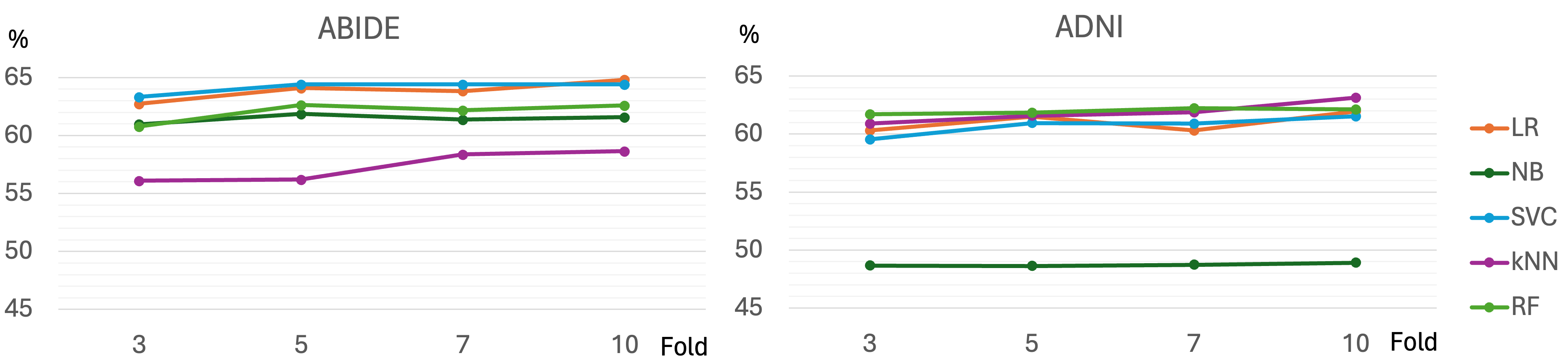
Figure 3: Test accuracy on ABIDE and ADNI with Schaefer when tuning training set size.

5.4 Sensitivity Study on Number of ROIs and Training Set Size

To assess the effect of the number of ROIs to model performance, we tune the number of ROIs on the Schaefer parcellation from {100, 200, 500, 1000} on the classification task. The results are reported in Table 7. Each model performs the best when the number of ROIs is set at 100 or 200.

We also test on different training set sizes by tuning $k$ in $k$-fold CV and report the results in Figure 3. The performance of each method improves with the increase in the training set size (larger $k$), which confirms the necessity of having datasets at this scale.

6 Conclusions, Limitations, and Future Directions

We release a functional brain network collection to the public at a large scale. The collection originates from 6 raw MRI image sources, covers 4 brain conditions, and totals to 2,702 subjects. Working with domain experts, we come up with a unified pipeline that converts raw fMRI and T1w images to brain networks. We tested the collection on 12 ML models and a recent graph analysis model to demonstrate that the data quality is not compromised while at the same time providing the results as domain baselines. We hope that the release of this collection of brain networks, together with the complete code of the processing pipeline, will promote both the development of graph-based models and the clinical advancement in the diagnosis and early intervention of neurodegenerative diseases.

We identify two limitations of this study: (1) Though the current brain network collection contains 2,702 subjects, it may still be considered small when applied to certain machine learning models (e.g., deep learning models). Due to the high computational cost, we are not able to produce a larger collection for now but will make continuous efforts in enriching the collection, (2) The current collection focuses on extracting brain networks from a single modality, that is, the functional MRI images. Recently, neuroimaging data lean towards the direction of combining different modalities such as diffusion and functional MRI for further integrated explorations of brain functionalities. The fusion of functional MRI and diffusion MRI can encode information regarding integrated activities of the human brain. In the future, we plan to work on the processing pipeline of diffusion MRI images to make multi-modal brain networks publicly accessible to the research community.

Appendix A Appendix

A.1 Dataset-related Details

A.1.1 Dataset Documentation

We provide a datasheet that documents this data collection (in the Supplementary materials).

A.1.2 Access Link and Data Repositories

The brain network datasets can be accessed at: https://doi.org/10.17608/k6.auckland.21397377.

We have a Github repository at https://github.com/brainnetuoa/data_driven_network_neuroscience which includes all our preprocessing codes and a demo on how to convert a raw fMRI image to a brain network in a step-by-step manner with sample input images from a subject in TaoWu.

Figshare (https://www.figshare.com) is a citable, shareable, and discoverable open data repository used by many educational institutions around the world, including ours. Figshare fits the many requirements of NeurIPS, including long term preservations of the data, access to a persistent identifier (an assigned DOI), and clear licensing and data standards.

A.1.3 Author Statement

As authors, we confirm that we bear all responsibility in case of any violation of rights during the collection of the data or other work, and will take appropriate action when needed, to remove data with such issues.

A.1.4 License of our Brain Network Datasets

CC BY-NC-SA 4.0

A.1.5 Consent Process for Neuroimages

ABIDE, TaoWu, and Neurocon all follow Creative Common licenses and their source neuroimages are open use. For ADNI and PPMI we have followed their policies (Data Usage and Publication Policy) on how to use and publish derived data and where appropriate, we have submitted our manuscripts for permission to publish. Both required proper acknowledgements of the entity and their funders in the paper, which we have included.

A.1.6 Computing Resources Used for Preprocessing

As stated in the main paper, fMRIPrep is computationally expensive. In our case, one run on one subject of fMRIPrep (with surface reconstruction enabled) using 8 threads on an Intel(R) Core(TM) i9-10940X CPU @ 3.30GHz takes on average 4-5 hours. Preprocessing of all data sources was split between two sites running on different internal cluster configurations. We are currently storing approximately 5 TB of data on these clusters, including the original neuroimages, preprocessed neuroimages, and our derived brain network data.

Site 1 cluster:

1. 3x Intel(R) Core(TM) i9-10940X CPU @ 3.30GHz

2. 1x Intel(R) Xeon(R) CPU ES-4020 v2 @ 2.60GHz

Site 2 cluster:

1. 5x Intel(R) Xeon(R) Silver 4314 CPU @ 2.40GHz

2. 1x Intel(R) Xeon(R) Gold 6230 CPU @ 2.10GHz

A.2 Experiment-related Details

A.2.1 Code

The code we used to run our entire pipeline and baseline experiments can be accessed on our Github: https://github.com/brainnetuoa/data_driven_network_neuroscience.

A.2.2 Parameters

As stated in the main paper we used scikit-learn for all our implementations and here we provide the full list of parameters (including those we used for Grid Search).

LogisticRegression(penalty:(’l1’, ’l2’, ’elasticnet’, ’none’), dual=False, tol=0.0001, C=1.0, fit_intercept=True, intercept_scaling=1, class_weight=None, random_state=None, solver=’lbfgs’, max_iter=1000000, multi_class=’auto’, verbose=0, warm_start=False, n_jobs=None, l1_ratio=None)

GaussianNB(priors=None, var_smoothing=1e-09)

SVC(C=1, kernel=(’rbf’,’linear’,’poly’,’sigmoid’,’shortest path’), degree=3, gamma=’auto’, coef0=0.0, shrinking=True, probability=False, tol=0.001, cache_size=200, class_weight=None, verbose=False, max_iter=- 1, decision_function_shape=’ovr’, break_ties=False, random_state=None)

KNeighborsClassifier(n_neighbors=5, weights=(’uniform’, ’distance’), algorithm=’auto’, leaf_size=30, p=(1,2), metric=’minkowski’, metric_params=None, n_jobs=None)

RandomForestClassifier(n_estimators=(50,100,150,200), criterion= ’entropy’, max_depth=5, min_samples_split=2, min_samples_leaf=1, min_weight_fraction_leaf=0.0, max_features=’sqrt’, max_leaf_nodes=None, min_impurity_decrease=0.0, bootstrap=True, oob_score=False, n_jobs=None, random_state=0, verbose=0, warm_start=False, class_weight=None, ccp_alpha=0.0, max_samples=None)

A.2.3 Computing Resources Used for Baselines

Experiments on baselines were performed on the internal cluster at site 2 (stated above).

A.2.4 Connectivity Measure Comparison on TaoWu

Table 8: Connectivity Measure Comparison - Classification Accuracy (mean$\pm$standard deviation)

TaoWu - AAL116
	Correlation	Covariance	Partial Correlation	Precision
Logistic Regression	82.5$\pm$12.7	82.5$\pm$12.7	62.5$\pm$5.0	65.0$\pm$12.2
Naïve Bayes	61.5$\pm$19.0	61.5$\pm$19.0	45.0$\pm$16.2	43.5$\pm$16.2
SVC	85.0$\pm$9.4	85.0$\pm$9.4	65.0$\pm$20.0	65.0$\pm$14.6
$k$NN	60.0$\pm$21.5	60.0$\pm$14.6	52.5$\pm$5.0	57.5$\pm$6.1
Random Forest	72.5$\pm$12.2	70.0$\pm$10.0	65.0$\pm$18.4	62.5$\pm$7.9

References

- [1] A repository of benchmark graph datasets for graph classification. https://github.com/GRAND-Lab/graph_datasets.
- [2] A. Abraham, F. Pedregosa, M. Eickenberg, P. Gervais, A. Mueller, J. Kossaifi, A. Gramfort, B. Thirion, and G. Varoquaux. Machine learning for neuroimaging with scikit-learn. Frontiers in neuroinformatics, 8:14, 2014.
- [3] P. S. Aisen, R. C. Petersen, M. Donohue, M. W. Weiner, A. D. N. Initiative, et al. Alzheimer’s disease neuroimaging initiative 2 clinical core: progress and plans. Alzheimer’s & Dementia, 11(7):734–739, 2015.
- [4] P. S. Aisen, R. C. Petersen, M. C. Donohue, A. Gamst, R. Raman, R. G. Thomas, S. Walter, J. Q. Trojanowski, L. M. Shaw, L. A. Beckett, et al. Clinical core of the alzheimer’s disease neuroimaging initiative: progress and plans. Alzheimer’s & Dementia, 6(3):239–246, 2010.
- [5] B. B. Avants, N. J. Tustison, G. Song, P. A. Cook, A. Klein, and J. C. Gee. A reproducible evaluation of ants similarity metric performance in brain image registration. Neuroimage, 54(3):2033–2044, 2011.
- [6] L. Badea, M. Onu, T. Wu, A. Roceanu, and O. Bajenaru. Exploring the reproducibility of functional connectivity alterations in parkinson’s disease. PLoS One, 12(11):e0188196, 2017.
- [7] D. S. Bassett and O. Sporns. Network neuroscience. Nature neuroscience, 20(3):353–364, 2017.
- [8] L. A. Beckett, M. C. Donohue, C. Wang, P. Aisen, D. J. Harvey, N. Saito, A. D. N. Initiative, et al. The alzheimer’s disease neuroimaging initiative phase 2: Increasing the length, breadth, and depth of our understanding. Alzheimer’s & Dementia, 11(7):823–831, 2015.
- [9] P. Bellec, S. Lavoie-Courchesne, P. Dickinson, J. P. Lerch, A. P. Zijdenbos, and A. C. Evans. The pipeline system for octave and matlab (PSOM): a lightweight scripting framework and execution engine for scientific workflows. Frontiers Neuroinformatics, 6:7, 2012.
- [10] I. Bilgen, G. Guvercin, and I. Rekik. Machine learning methods for brain network classification: Application to autism diagnosis using cortical morphological networks. Journal of neuroscience methods, 343:108799, 2020.
- [11] T. Bonald, N. de Lara, Q. Lutz, and B. Charpentier. Scikit-network: Graph analysis in python. J. Mach. Learn. Res., 21(185):1–6, 2020.
- [12] X. Bresson and T. Laurent. Residual gated graph convnets. arXiv preprint arXiv:1711.07553, 2017.
- [13] J. Cadena, A. K. Vullikanti, and C. C. Aggarwal. On dense subgraphs in signed network streams. In 2016 IEEE 16th International Conference on Data Mining (ICDM), pages 51–60. IEEE, 2016.
- [14] S. Chen, Z. He, X. Han, X. He, R. Li, H. Zhu, D. Zhao, C. Dai, Y. Zhang, Z. Lu, et al. How big data and high-performance computing drive brain science. Genomics, proteomics & bioinformatics, 17(4):381–392, 2019.
- [15] J. Chung, C. Gulcehre, K. Cho, and Y. Bengio. Empirical evaluation of gated recurrent neural networks on sequence modeling. arXiv preprint arXiv:1412.3555, 2014.
- [16] R. W. Cox. Afni: Software for analysis and visualization of functional magnetic resonance neuroimages. Computers and Biomedical Research, 29(3):162–173, 1996.
- [17] C. Craddock, Y. Benhajali, C. Chu, F. Chouinard, A. Evans, A. Jakab, B. S. Khundrakpam, J. D. Lewis, Q. Li, M. Milham, et al. The neuro bureau preprocessing initiative: open sharing of preprocessed neuroimaging data and derivatives. Frontiers in Neuroinformatics, 7, 2013.
- [18] V. P. Dwivedi, C. K. Joshi, A. T. Luu, T. Laurent, Y. Bengio, and X. Bresson. Benchmarking graph neural networks. arXiv preprint arXiv:2003.00982, 2020.
- [19] F. Errica, M. Podda, D. Bacciu, and A. Micheli. A fair comparison of graph neural networks for graph classification. arXiv preprint arXiv:1912.09893, 2019.
- [20] O. Esteban, C. J. Markiewicz, R. W. Blair, C. A. Moodie, A. I. Isik, A. Erramuzpe, J. D. Kent, M. Goncalves, E. DuPre, M. Snyder, et al. fmriprep: a robust preprocessing pipeline for functional mri. Nature methods, 16(1):111–116, 2019.
- [21] F. V. Farahani, W. Karwowski, and N. R. Lighthall. Application of graph theory for identifying connectivity patterns in human brain networks: a systematic review. frontiers in Neuroscience, 13:585, 2019.
- [22] B. Fischl. Freesurfer. NeuroImage, 62(2):774–781, 2012. 20 YEARS OF fMRI.
- [23] A. Fornito, A. Zalesky, and E. Bullmore. Fundamentals of brain network analysis. Academic Press, 2016.
- [24] M. D. Fox and M. Greicius. Clinical applications of resting state functional connectivity. Frontiers in systems neuroscience, 4:19, 2010.
- [25] M. D. Fox, A. Z. Snyder, J. L. Vincent, M. Corbetta, D. C. Van Essen, and M. E. Raichle. The human brain is intrinsically organized into dynamic, anticorrelated functional networks. Proceedings of the National Academy of Sciences, 102(27):9673–9678, 2005.
- [26] M. D. Fox, D. Zhang, A. Z. Snyder, and M. E. Raichle. The global signal and observed anticorrelated resting state brain networks. Journal of neurophysiology, 101(6):3270–3283, 2009.
- [27] K. J. Gorgolewski, T. Auer, V. D. Calhoun, R. C. Craddock, S. Das, E. P. Duff, G. Flandin, S. S. Ghosh, T. Glatard, Y. O. Halchenko, et al. The brain imaging data structure, a format for organizing and describing outputs of neuroimaging experiments. Scientific data, 3(1):1–9, 2016.
- [28] W. L. Hamilton, R. Ying, and J. Leskovec. Inductive representation learning on large graphs. In Proceedings of the 31st International Conference on Neural Information Processing Systems, pages 1025–1035, 2017.
- [29] S. Haykin. Neural networks: a comprehensive foundation. Prentice Hall PTR, 1998.
- [30] M. Ingalhalikar, S. Shinde, A. Karmarkar, A. Rajan, D. Rangaprakash, and G. Deshpande. Functional connectivity-based prediction of autism on site harmonized abide dataset. IEEE Transactions on Biomedical Engineering, 68(12):3628–3637, 2021.
- [31] M. Jenkinson, C. F. Beckmann, T. E. Behrens, M. W. Woolrich, and S. M. Smith. Fsl. NeuroImage, 62(2):782–790, 2012. 20 YEARS OF fMRI.
- [32] J. Kawahara, C. J. Brown, S. P. Miller, B. G. Booth, V. Chau, R. E. Grunau, J. G. Zwicker, and G. Hamarneh. Brainnetcnn: Convolutional neural networks for brain networks; towards predicting neurodevelopment. NeuroImage, 146:1038–1049, 2017.
- [33] T. N. Kipf and M. Welling. Semi-supervised classification with graph convolutional networks. arXiv preprint arXiv:1609.02907, 2016.
- [34] T. Lanciano, F. Bonchi, and A. Gionis. Explainable classification of brain networks via contrast subgraphs. In Proceedings of the 26th ACM SIGKDD International Conference on Knowledge Discovery & Data Mining, pages 3308–3318, 2020.
- [35] Y. LeCun, B. Boser, J. Denker, D. Henderson, R. Howard, W. Hubbard, and L. Jackel. Handwritten digit recognition with a back-propagation network. Advances in neural information processing systems, 2, 1989.
- [36] X. Li, P. S. Morgan, J. Ashburner, J. Smith, and C. Rorden. The first step for neuroimaging data analysis: Dicom to nifti conversion. Journal of neuroscience methods, 264:47–56, 2016.
- [37] J. Liu, Y. Sheng, W. Lan, R. Guo, Y. Wang, and J. Wang. Improved asd classification using dynamic functional connectivity and multi-task feature selection. Pattern Recognition Letters, 138:82–87, 2020.
- [38] Y. Liu, Y. Liu, and K. Chan. Ordinal regression via manifold learning. Proceedings of the AAAI Conference on Artificial Intelligence, 25(1):398–403, Aug. 2011.
- [39] J. MacQueen et al. Some methods for classification and analysis of multivariate observations. In Proceedings of the fifth Berkeley symposium on mathematical statistics and probability, volume 1, pages 281–297. Oakland, CA, USA, 1967.
- [40] N. Makris, J. M. Goldstein, D. Kennedy, S. M. Hodge, V. S. Caviness, S. V. Faraone, M. T. Tsuang, and L. J. Seidman. Decreased volume of left and total anterior insular lobule in schizophrenia. Schizophrenia research, 83(2-3):155–171, 2006.
- [41] K. Marek, D. Jennings, S. Lasch, A. Siderowf, C. Tanner, T. Simuni, C. Coffey, K. Kieburtz, E. Flagg, S. Chowdhury, et al. The parkinson progression marker initiative (ppmi). Progress in neurobiology, 95(4):629–635, 2011.
- [42] C. Morris, N. M. Kriege, F. Bause, K. Kersting, P. Mutzel, and M. Neumann. Tudataset: A collection of benchmark datasets for learning with graphs. arXiv preprint arXiv:2007.08663, 2020.
- [43] S. Noble, D. Scheinost, E. S. Finn, X. Shen, X. Papademetris, S. C. McEwen, C. E. Bearden, J. Addington, B. Goodyear, K. S. Cadenhead, et al. Multisite reliability of mr-based functional connectivity. Neuroimage, 146:959–970, 2017.
- [44] S. Parisot, S. I. Ktena, E. Ferrante, M. Lee, R. G. Moreno, B. Glocker, and D. Rueckert. Spectral graph convolutions for population-based disease prediction. In International conference on medical image computing and computer-assisted intervention, pages 177–185. Springer, 2017.
- [45] F. Pedregosa, G. Varoquaux, A. Gramfort, V. Michel, B. Thirion, O. Grisel, M. Blondel, P. Prettenhofer, R. Weiss, V. Dubourg, J. Vanderplas, A. Passos, D. Cournapeau, M. Brucher, M. Perrot, and E. Duchesnay. Scikit-learn: Machine learning in Python. Journal of Machine Learning Research, 12:2825–2830, 2011.
- [46] Z. Rakhimberdina, X. Liu, and T. Murata. Population graph-based multi-model ensemble method for diagnosing autism spectrum disorder. Sensors, 20(21):6001, 2020.
- [47] A. Schaefer, R. Kong, E. M. Gordon, T. O. Laumann, X.-N. Zuo, A. J. Holmes, S. B. Eickhoff, and B. T. Yeo. Local-global parcellation of the human cerebral cortex from intrinsic functional connectivity mri. Cerebral cortex, 28(9):3095–3114, 2018.
- [48] C. Tsourakakis, F. Bonchi, A. Gionis, F. Gullo, and M. Tsiarli. Denser than the densest subgraph: extracting optimal quasi-cliques with quality guarantees. In Proceedings of the 19th ACM SIGKDD international conference on Knowledge discovery and data mining, pages 104–112, 2013.
- [49] N. Tzourio-Mazoyer, B. Landeau, D. Papathanassiou, F. Crivello, O. Etard, N. Delcroix, B. Mazoyer, and M. Joliot. Automated anatomical labeling of activations in spm using a macroscopic anatomical parcellation of the mni mri single-subject brain. Neuroimage, 15(1):273–289, 2002.
- [50] P. Veličković, G. Cucurull, A. Casanova, A. Romero, P. Lio, and Y. Bengio. Graph attention networks. arXiv preprint arXiv:1710.10903, 2017.
- [51] J. H. Ward Jr. Hierarchical grouping to optimize an objective function. Journal of the American statistical association, 58(301):236–244, 1963.
- [52] M. W. Weiner, D. P. Veitch, P. S. Aisen, L. A. Beckett, N. J. Cairns, R. C. Green, D. Harvey, C. R. Jack Jr, W. Jagust, J. C. Morris, et al. The alzheimer’s disease neuroimaging initiative 3: Continued innovation for clinical trial improvement. Alzheimer’s & Dementia, 13(5):561–571, 2017.
- [53] K. Xu, W. Hu, J. Leskovec, and S. Jegelka. How powerful are graph neural networks? In International Conference on Learning Representations, 2018.
- [54] C. Yan and Y. Zang. Dparsf: a matlab toolbox for" pipeline" data analysis of resting-state fmri. Frontiers in systems neuroscience, page 13, 2010.
- [55] X. Zhang, J. Huang, Y. Yang, X. He, R. Liu, and N. Zhong. Applying python in brain science education. In 2019 International Joint Conference on Information, Media and Engineering (IJCIME), pages 396–400. IEEE, 2019.