Abstract

Meta-learning of numerical algorithms for a given task consists of the data-driven identification and adaptation of an algorithmic structure and the associated hyperparameters. To limit the complexity of the meta-learning problem, neural architectures with a certain inductive bias towards favorable algorithmic structures can, and should, be used. We generalize our previously introduced Runge–Kutta neural network to a recursively recurrent neural network (R2N2) superstructure for the design of customized iterative algorithms. In contrast to off-the-shelf deep learning approaches, it features a distinct division into modules for generation of information and for the subsequent assembly of this information towards a solution. Local information in the form of a subspace is generated by subordinate, inner, iterations of recurrent function evaluations starting at the current outer iterate. The update to the next outer iterate is computed as a linear combination of these evaluations, reducing the residual in this space, and constitutes the output of the network. We demonstrate that regular training of the weight parameters inside the proposed superstructure on input/output data of various computational problem classes yields iterations similar to Krylov solvers for linear equation systems, Newton-Krylov solvers for nonlinear equation systems, and Runge–Kutta integrators for ordinary differential equations. Due to its modularity, the superstructure can be readily extended with functionalities needed to represent more general classes of iterative algorithms traditionally based on Taylor series expansions.

• Institute of Energy and Climate Research, Energy Systems Engineering (IEK-10), Forschungszentrum Jülich GmbH, Jülich 52425, Germany

• RWTH Aachen University Aachen 52062, Germany

• JARA-ENERGY, Jülich 52425, Germany

• RWTH Aachen University, Process Systems Engineering (AVT.SVT), Aachen 52074, Germany

• Department of Mathematics, National University of Singapore, Singapore

• Department of Informatics, Technical University of Munich, Boltzmannstr. 3, 85748 Garching b. Munich, Germany

• Departments of Applied Mathematics and Statistics & Chemical and Biomolecular Engineering, Johns Hopkins University, Baltimore, Maryland 21218, USA

Keywords: Numerical Analysis, Meta-Learning, Machine Learning, Runge-Kutta Methods, Newton-Krylov Solvers, Data-driven Algorithm Design

1 Introduction

The relationship between a class of residual recurrent neural networks (RNN) and numerical integrators has been known since Rico-Martinez et al., (1992) proposed the architecture shown in Figure 1(a) for nonlinear system identification. Together with more recent work of the authors (Mitsos et al.,, 2018; Guo et al.,, 2022) it motivates the present work. The salient point of the RNN proposed by Rico-Martinez et al., (1992) is that it provides the structure of an integrator, in that case a fourth-order explicit Runge–Kutta (RK) scheme, within which the right-hand-side (RHS) of an ordinary differential equation (ODE) can be approximately learned from time series data. To this end, the integrator is essentially hard-wired in the forward pass of the RNN – a first instance of the body of work nowadays referred to as “neural ordinary differential equations” (Chen et al.,, 2018). However, upon closer inspection, the architecture reveals a complementary utility: When the model equations are known, it is the structure and weights associated with an algorithm that can be discovered, see Figure 1(b). We study the latter setting in this work.

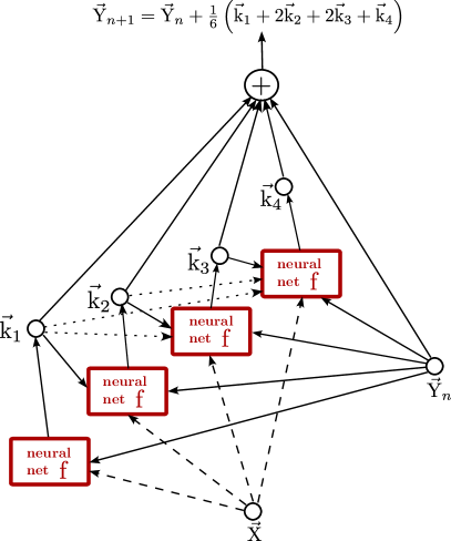
(a) When the architecture and integrator weights are hard-wired (black connections and their weights), a model of the unknown system (thick red squares) can be approximated, e.g., by multi-layer perceptrons.

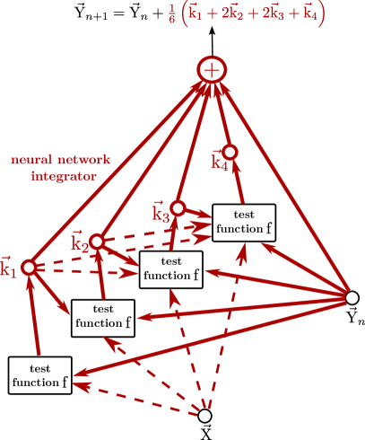
(b) When the model equations are known (black squares), the structure and weights (thick red connections and their weights) associated with a solution algorithm can be discovered for that system.

Figure 1: A recurrent neural network architecture templated on Runge–Kutta integrators, adapted from Rico-Martinez et al., (1992). The illustration shows the classical fourth-order Runge–Kutta scheme, where $\vec{\mathrm{Y}}$ and $\vec{\mathrm{X}}$ are the dependent and independent variables, respectively, $\mathrm{f}$ is the RHS of an ODE, and $\vec{\mathrm{k}}_{i}$ are stage values. Recurrent function evaluations are computed internally, and the network itself can be applied iteratively via external recurrence. Given input and output data for training, a model (a) or an algorithm (here, an initial value solver) for that model (b) can be learned.

Algorithms encoded by this architecture inherit two structural features from a RK scheme: i) they are based on recurrent function evaluations (inner recurrence), and ii) they compute iterates by adding a weighted sum of these inner evaluations that acts as correction to the input (outer recurrence). One critical observation is that such nested recurrent features also characterize (matrix)-free Krylov subspace methods such as restarted GMRES (Saad and Schultz,, 1986) or Newton–Krylov–GMRES (Kelley,, 1995), where finite differences (i.e., linear combinations) between recurrent function evaluations provide estimates of directional derivatives in various directions. This estimation of derivatives, or, more broadly, of Taylor series as in the RK case, forms the backbone of either of these two classical algorithm families, RK and Krylov methods. Observing these parallels, we conjecture that a recursively recurrent neural network (R2N2) can approximate many traditional numerical algorithms based on Taylor series expansions.

Returning to Figure 1(b), we see that the (hyper-)parameters of the R2N2 are naturally linked to those of the algorithm it furnishes, e.g., weights connecting to the output can encode quadratures, and the internal recurrence count determines the number of function evaluations and the dimension of the subspace that is generated. It is this particular connectivity, highlighted in red, that is subject to discovery, whether it be encoding a Butcher tableau in the case of RK (Butcher,, 2016; Guo et al.,, 2022) or finding the combination of weights that convert function evaluations into directional derivatives for Newton–Krylov (NK).

The question that motivates this work is thus: Can meta-learning applied to the architecture and parameters of the R2N2 discover old and new algorithms “personalized” to certain problem classes? We advocate that the R2N2 provides an architecture search space particularly suited for answering this question. The parameters of the R2N2 can be partitioned a priori into those that are hard-wired and those subject to meta-learning. We can focus on the discrete features, i.e., determining the operations and connections that yield a best performant algorithm, or on the (continuous) weights, i.e., on how to best combine these operations. The former is also referred to as algorithm configuration, while the latter is a special case of parameter tuning (Hoos,, 2011). Algorithm configuration has been optimized in a previous effort of the authors (Mitsos et al.,, 2018), albeit for a different, less expressive architecture with all weight parameters collapsed into a scalar stepsize. More recently, we worked with a fixed architecture as in Figure 1(b) such that Butcher tableaus personalized to specific classes of initial-value problems (IVPs) were learned (Guo et al.,, 2022). The present work seeks to extend this latter application to further numerical algorithms, in particular NK, and to thereby demonstrate that the R2N2 gives rise to a potent superstructure for optimal algorithm discovery. In follow-up work, we aim to show that jointly optimizing the weights and architecture from such a superstructure realizes learning of optimal iterative numerical algorithms, and to explore the use of approximate physical models as preconditioners within the superstructure.

1.1 Related work

Automated algorithm configuration and tuning dates back to Rice, (1976) and studies meta-algorithms or meta-heuristics that pick the best algorithm from a set of (parametrized) algorithms for certain problem classes by manipulating the (hyper)parameters of a solver (Hoos,, 2011). Speed-ups up to a factor of $50$ have been demonstrated, e.g., for satisfiability problems (KhudaBukhsh et al.,, 2016) or mixed-integer problems (Hutter et al.,, 2010) by leveraging problem structure. This is in contrast to classical numerical algorithms that are designed to work with little or no a priori knowledge about the internal structure of the problem instances to be solved, and are often biased towards worst-case performance criteria (Gupta and Roughgarden,, 2020). In contrast, algorithms adapted to specific problem classes typically incur a generalization weakness on other problems (Wolpert and Macready,, 1997). Mitsos et al., (2018) modeled algorithms as feedback schemes with a cost ascribed to each operation, such that the design of iterative algorithms was posed as an optimal control problem of mixed-integer nonlinear (MINLP) type. They restricted operations to monomials of function evaluations and derivatives, thus specifying a family of algorithms. Depending on the analyzed problem, the procedure would recover known, established algorithms from this family, but also new algorithms that were optimal for the problems considered.

Mitsos et al., (2018) solved the algorithm generation MINLPs via the deterministic global solver BARON (Tawarmalani and Sahinidis,, 2005). Possible gains of tailored algorithms must be weighed up against the required effort for finding them. Machine learning (ML) can decrease this effort. This has recently been demonstrated forcefully by Fawzi et al., (2022) who improved the best known algorithms on several instances of matrix multiplication, an NP-hard problem, and Mankowitz et al., (2023) who found new state-of-the-art sorting algorithms, both using deep reinforcement learning built on top of the AlphaZero framework (Silver et al.,, 2018). This landmark achievement is expected to spur new interest in algorithm discovery via ML. ML methods can optimize the performance of algorithms on a problem class implicitly given through data (Balcan,, 2020; Gupta and Roughgarden,, 2020). Such data-driven algorithm design has been applied to several computational problems, e.g., learning to solve graph-related problems (e.g., (Tang et al.,, 2020)), learning sorting algorithms (e.g., (Schwarzschild et al.,, 2021)), learning to branch (Khalil et al.,, 2016; Balcan et al.,, 2018), meta-learning optimizers (e.g., (Andrychowicz et al.,, 2016; Metz et al.,, 2020)), and our previous work of meta-learning RK integrators (Guo et al.,, 2022). In the context of this problem, the R2N2 defines a superstructure for a class of iterative algorithms. The notion of superstructure is used in many disciplines to denote a union of structures that are candidate solutions to a problem, e.g., in optimization-based flowsheet design within process systems engineering (Yeomans and Grossmann,, 1999; Mencarelli et al.,, 2020). In general, optimizing a superstructure requires integer optimization techniques as in Mitsos et al., (2018). Given the neural network interpretation of the R2N2, however, (heuristic) methods for neural architecture search, e.g., (Elsken et al., 2019a, ; Li et al., 2021a, ), may be considered. Consequently, the optimal algorithmic procedure corresponds to an optimized neural architecture. In this work, we avoid integer optimization by essentially fixing the neural architecture for each respective numerical experiment, and optimizing the weights therein.

The R2N2 belongs to the class of recurrent neural networks (RNNs), which are a natural fit for iterative algorithms. For instance, RNN architectures templated on RK integrators have been suggested several decades ago (Rico-Martinez et al.,, 1992, 1994, 1995; González-García et al.,, 1998). These architectures can be used for both, computing the outputs of an integrator, e.g., (Rico-Martinez et al.,, 1992; González-García et al.,, 1998) and identifying terms in a differential equation, e.g., (Rico-Martinez et al.,, 1994; Nascimento et al.,, 2020; Lovelett et al.,, 2020; Zhao and Mau,, 2020; Goyal and Benner,, 2021). Further, as the RK network of Rico-Martinez et al., (1992) learns the residual between the input and the output data, it constitutes the first occurrence of a residual network (ResNet, He et al., (2016)). Several newer ResNet-based architectures retain structural similarities with numerical methods (Lu et al.,, 2018). For instance, FractalNet (Larsson et al.,, 2017) resembles higher-order RK schemes in its macrostructure, as does the ResNet-derived architecture by Schwarzschild et al., (2021). Lu et al., (2018) proposed a ResNet augmented by a module derived from linear multistep methods (Butcher,, 2016). Beyond architectural similarity with numerical methods, neural networks proposed in literature can also be designed such that the mathematical mapping they represent shares desirable properties with that of a method, e.g., symplectic mappings (Jin et al.,, 2020) for symplectic integrators or contracting layers (Chevalier et al.,, 2021) for fixed-point iterations. Dufera, (2021) and Guo et al., (2022) trained networks to match the derivatives of ODEs or of their RK-based solution expansion at training points, respectively. Finally, direct learning of algorithms from neural network-like graphs has been proposed, e.g., by Tsitouras, (2002), Denevi et al., (2018), Mishra, (2018) and Venkataraman and Amos, (2021).

Contributions

We build on the RK-NN of our previous work (Guo et al.,, 2022) and introduce the R2N2 superstructure for iterative numerical algorithms. The function to be evaluated inside the R2N2 architecture is itself explicitly given as part of the input problem instance, which is a major difference to operator networks that learn parameter-to-solution mappings like those in Lu et al., (2019) and Li et al., 2021b . Thus, higher-order iterative algorithms for equation solving and numerical integration, that are traditionally constructed through Taylor series expansion, can be approximated by the R2N2 superstructure. We demonstrate that both NK methods for solving systems of equations and RK methods for solving IVPs are encompassed by the proposed R2N2 as a joint superstructure. Further, in numerical experiments we show that the trained R2N2 can match, and sometimes improve upon, the iterations performed by NK and RK algorithms for a given number of function evaluations. A comparison of the R2N2 to GMRES on linear equation systems – which are the basic building block of iterative solvers for nonlinear systems – provides insight into the operations of the R2N2. In these experiments, our particular realization of this superstructure has a strong inductive bias that alleviates the need for certain configuration decisions, i.e., integer optimization, in algorithm design. The weights that remain to be trained correspond to coefficients or hyperparameters of the algorithms in question, and we tune these using PyTorch (Paszke et al.,, 2019).

The remainder of this article is structured as follows. In Section 2, we give a general problem definition for learning algorithms from task data and specify the problem for iterative algorithms. Section 3 introduces the R2N2 superstructure for learning iterative algorithms and shows its relation to steps of iterative equation solvers and integrators. Section 4 presents results of numerical experiments, where the R2N2 is trained to perform iterations of linear and nonlinear equation solvers and integrators. We summarize our results in Section 5 and discuss future research opportunities in Section 6.

2 Problem definition

Various generic problem formulations for learning algorithms from problem data exist in the literature, e.g., in Balcan, (2020), Gupta and Roughgarden, (2020), and our prior work (Guo et al.,, 2022). This section provides background and notation for a generic algorithm learning problem, Section 2.1, and specifies the problem formulation for learning iterative algorithms, Section 2.2.

2.1 Generic problem formulation

Let $\mathbf{x}\in\mathbb{R}^{m}$ and $\mathcal{F}$ a set of vectors such that $F\in\mathcal{F}$ is a problem instance composed of a continuous function $\bm{f}\vcentcolon\mathbb{R}^{m}\mapsto\mathbb{R}^{m}$ and some optional, additional problem parameters $\mathbf{p}$, e.g., time, such that we can write $F=\left(\bm{f},\mathbf{p}\right)$. Then, a traditional class of problems can be characterized by a functional $\Pi$ acting on $F$ and a point in $\mathbb{R}^{m}$. Further, a solution of $F$ is any $\mathbf{x}^{\star}\in\mathbb{R}^{m}$ for which

$$\Pi(\mathbf{x}^{\star},F)=0.$$ (1)

This abstract form encompasses many problem types. The first type we consider here is finding the solution $\mathbf{x}^{\star}$ of algebraic equations, s.t

$$\Pi(\mathbf{x}^{\star},F)=\left\|\bm{f}(\mathbf{x}^{\star})\right\|=0.$$ (2)

The second problem type is finding the solution of initial-value problems (IVPs) for a specific end time $t$, s.t.

$$\Pi(\mathbf{x}^{\star},F)=\left\|\mathbf{y}_{0}+\int_{\tau=t_{0}}^{\tau=t}\bm{f}(\mathbf{y}(\tau))d\tau-\mathbf{x}^{\star}\right\|=0,$$ (3)

where $\bm{f}$ is the RHS of an ODE and $\mathbf{y}(\tau)\in\mathbb{R}^{m}$ is the state of the system at time $\tau$ with the initial value $\mathbf{y}_{0}=\mathbf{y}(\tau=t_{0})$. Equation (3) illustrates the definition of a problem instance and optional parameters $\mathbf{p}$, where $\mathbf{p}=\left(\mathbf{y}_{0},t\right)$. The solution is the final value of the states, i.e., $\mathbf{x}^{\star}=\mathbf{y}(\tau=t)$.

We only consider problem instances $F$ for which a solution $\mathbf{x}^{\star}$ exists. Then, we call any operator mapping $F\mapsto\mathbf{x}^{\star}$ a solver $\mathcal{S}(F)$. In general, we do not explicitly know these solvers and hence need to approximate their action by the design and use of numerical algorithms. That is, algorithms act as approximate solvers $\mathcal{A}(F,\bm{\uptheta})\approx\mathcal{S}(F)$, parametrized by $\bm{\uptheta}$, such that

$$\Pi\left(\mathcal{A}(F,\bm{\uptheta}),F\right)\leq\delta,$$

where $\delta\in\mathbb{R}^{+}$ is sufficiently small and ideally user-defined. The challenge of designing numerical methods pertains to finding a structure linking mathematical operations parametrized by a set of parameters $\bm{\uptheta}$, which together yield performant solvers for problems that can be recast to Problem (1).

Due to the effort expended in designing algorithms, another important consideration is the range of applicability of the algorithm, i.e., the size of the set of problems it can solve. Traditional algorithms for problems like (2) and (3) often consider a certain worst-case performance in a given problem class $\mathcal{F}$. In contrast, we are interested in the average/expected performance of algorithms over a specific problem class, which is defined by a distribution $\mu$ over $\mathcal{F}$. Then, finding performant, or even optimal, algorithms for such a class of problems requires solving

$$\operatorname{min}_{\bm{\uptheta}}\mathbb{E}_{\mu}\left[\left\|\Pi\left(\mathcal{A}(F,\bm{\uptheta}),F\right)\right\|\right]+R(\mathcal{A}(F,\bm{\uptheta}),\bm{\uptheta}).$$ (4)

Problem (4) seeks parameters $\bm{\uptheta}$ which minimize the expectation of the residual norm of solutions computed to Equation (1) using $\mathcal{A}(F,\bm{\uptheta})$ over problem instances distributed according to $\mu$. The second term in (4), $R(\mathcal{A}(F,\bm{\uptheta}),\bm{\uptheta})$, is reserved for some additional regularization penalty that can promote certain properties in the approximate solution $\mathcal{A}(\cdot,\bm{\uptheta}^{\star})$, such as a desired convergence order (Guo et al.,, 2022). The regularization can also penalize the parameter values $\bm{\uptheta}$ directly, e.g., in $L_{2}$ regularization. The algorithmic structure itself can be described by discrete variables, e.g., to indicate whether an operation or module exists in the algorithm. However, to include such discrete variables one requires a metric that determines which structure is optimal. This is typically assessed over a prolonged number of iterations and requires integer optimization techniques, see, e.g., Mitsos et al., (2018). In this work, the goal is rather to demonstrate that the iterations of several iterative algorithms have a common superstructure. Consequently, we focus on tuning the parameters of this superstructure towards different problem classes. Thus, Problem (4) resembles a regular multi-task learning problem in the context of statistical learning (Baxter,, 2000), where tasks are equated with problem instances $F$. To handle such a problem, the expectation term can be approximated by drawing samples of task data from $\mu$ and minimizing some loss function for them.

2.2 Iterative numerical algorithms

We focus on iterative algorithms, which construct a sequence of iterates $\{\mathbf{x}_{k}\}$ approaching a solution of $F$. Starting with the initial point $\mathbf{x}_{0}$, the algorithm computes new iterates by applying

$$\mathbf{x}_{k+1}=\mathcal{A}^{iter}(F,\bm{\uptheta};\mathbf{x}_{k}),$$ (5)

such that the sequence ideally converges to some $\hat{\mathbf{x}}$:

$$\hat{\mathbf{x}}=\lim\limits_{k\rightarrow\infty}{\mathbf{x}_{k}}.$$

If we have $\Pi(\hat{\mathbf{x}},F)=0$, then $\mathcal{A}^{iter}$ is convergent to the solution of $F$.

In the following, we restrict the possible realizations of $\mathcal{A}^{iter}$ strongly by narrowing our attention to iterative algorithms that apply additive step updates in a generalized Krylov-type subspace $\mathcal{K}_{n}$. This subspace is spanned by vectors $\mathbf{v}_{0},\ldots,\mathbf{v}_{n-1}$, i.e.,

$$\mathcal{K}_{n}(\bm{f},\mathbf{x})=\operatorname{\mathrm{span}}\{\mathbf{v}_{0},\mathbf{v}_{1},\ldots,\mathbf{v}_{n-1}\},$$ (6)

that are generated by recurrent function evaluations at $\mathbf{x}_{k}$, i.e.,

$$\mathbf{v}_{0}\vcentcolon=\bm{f}\left(\mathbf{x}_{k}\right),$$ (7a)

$$\mathbf{v}_{j}=\bm{f}\left(\mathbf{x}_{k}+\sum_{l=0}^{j-1}b_{jl}\mathbf{v}_{l}\right),\quad j=1,\ldots,n-1,$$ (7b)

for some $b_{jl}\in\mathbb{R}$. The next iterate $\mathbf{x}_{k+1}$ is computed by adding a linear combination of this basis to $\mathbf{x}_{k}$, i.e.,

$$\mathbf{x}_{k+1}=\mathbf{x}_{k}+\sum_{j=0}^{n-1}c_{j}\mathbf{v}_{j},$$ (8)

for some $c_{j}\in\mathbb{R}$. Equation (7b) describes an inner iteration of the algorithm, while Equation (8) constitutes an outer iteration. Together, Equations (7)—(8) define a common superstructure for iterative algorithms. This structure has parallels to Krylov subspace methods (Saad,, 2003), and RK methods (Butcher,, 2016), respectively, see Section 3.2.

Considering only iterative algorithms within this superstructure has several advantages compared to alternatives that rely on deep learning with heavily parametrized models. First, the iterative nature of the superstructure greatly reduces the total amount of parameters needed to learn solution procedures. Second, Equations (7) and (8) eliminate most of the functional forms admissible under Equation (5). And third, directly embedding $\bm{f}$ in the superstructure avoids the need to learn an extra representation of the problem within the solver mapping. The resulting superstructure resembles an RNN, and automatic differentiation frameworks for the training of neural networks such as PyTorch (Paszke et al.,, 2019) can be used to determine the remaining free parameters $\bm{\uptheta}$.

3 R2N2 superstructure for iterative algorithms

We recently proposed the RK-NN, a neural network architecture templated on RK integrators, to personalize coefficients of a RK method to a specific problem class (Guo et al.,, 2022). In this work, we extend our view of the RK-NN to that of a more general superstructure for iterative numerical algorithms, the R2N2, that is applicable to different problem classes such as equation solving and numerical integration. Section 3.1 describes the architecture of the R2N2. Each forward pass through the R2N2 is interpreted as an iteration of a numerical algorithm (outer recurrence) that invokes one or many recurrent function evaluations (inner recurrence), starting at the current iterate, to compute the next iterate. The R2N2 is equivalent to the RK-NN from Guo et al., (2022) for the specific case of minimizing empirical risk (Problem (4)) for classes of IVPs, Problem (3). However, as a small addition to the original RK-NN, the R2N2 superstructure now allows presetting various routines for function evaluation, see supplementary material (SM1). In Section 3.2, we show that the applicability of the R2N2 as a superstructure is substantially extended beyond the case of solving IVPs. Section 3.3 and Section 3.4 conclude this section with remarks about training and implementation of the R2N2 superstructure.

3.1 Neural architecture underlying the R2N2 superstructure

The proposed R2N2 superstructure is portrayed by Figure 2. It represents the computation of one iteration of a numerical algorithm, i.e., the mathematical function defined by the RNN architecture can substitute for $\mathcal{A}^{iter}(F,\bm{\uptheta};\mathbf{x}_{k})$ in Equation (5), where a problem instance $F$ contains $\bm{f}$ and $\mathbf{p}$. Each step requires the current iterate $\mathbf{x}_{k}$ as an input, where the initial $\mathbf{x}_{0}$ is typically supplied within $\mathbf{p}$. Further, a function $\bm{f}\vcentcolon\mathbb{R}^{m}\mapsto\mathbb{R}^{m}$ is prescribed externally as part of a task, but remains unchanged for all iterates. Finally, a parameter $h$ for scaling of the layer computations is part of the input to the superstructure. For some problem classes, we choose $h$ according to problem parameters $\mathbf{p}$, e.g., the timestep in integration. Whenever $h$ is not specified, assume $h=1$, i.e., no scaling.

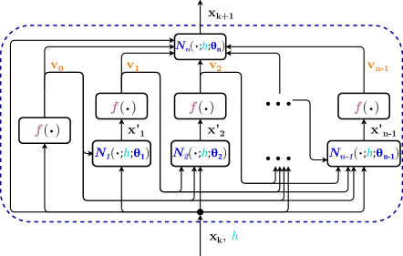
Figure 2: Proposed recursively recurrent neural network-based superstructure of an iterative algorithm. The recurrent cell is delimited by the dashed blue line and computes $\mathbf{x}_{k+1}$ as a function of the current iterate $\mathbf{x}_{k}$, a scaling parameter $h$ (cyan), and a function $\bm{f}$ (magenta). Trainable weights $\bm{\uptheta}_{j}$ are contained within each of the layer modules $\bm{N}_{j}$ with $j=1,2,\ldots,n-1$. $\bm{\uptheta}_{n}$ denote the trainable weights of the output module $\bm{N}_{n}$ (all in blue). $\mathbf{x}_{k}$ has a skip connection to each layer and to the output module. Intermediate function arguments, i.e., inputs to $\bm{f}$ in layer $j$, are called $\mathbf{x}^{\prime}_{j}$ and subspace members, i.e., outputs of $\bm{f}$ in layer $j$, are denoted by $\mathbf{v}_{j}$ (orange).

The initial layer, which is the left-most in Figure 2, is always a direct function evaluation at the current iterate, $\bm{f}(\mathbf{x}_{k})$, i.e., we have $\mathbf{v}_{0}=\bm{f}(\mathbf{x}_{k})$. The remaining $n-1$ layers of the superstructure each output a $\mathbf{v}_{j}$, $j=1,\ldots,n-1$ by applying a composition of $\bm{f}$ and $\bm{N}_{j}$. $\bm{N}_{j}$ linearly combines its inputs $\mathbf{v}_{0},\ldots,\mathbf{v}_{j-1}$ using trainable parameters $\bm{\uptheta}_{j}$ and, scales the term with $h$ and adds it to $\mathbf{x}_{k}$ to provide $\mathbf{x}^{\prime}_{j}$, the input to $\bm{f}$ in the $j$-th layer:

$$\mathbf{x}^{\prime}_{j}=\bm{N}_{j}\left(\mathbf{x}_{k};\mathbf{v}_{0},\ldots,\mathbf{v}_{j-1};h\right)=\mathbf{x}_{k}+h\sum_{l=0}^{j-1}\theta_{j,l}\mathbf{v}_{l}$$ (9)

The $\{\mathbf{v}_{j}\}$, including $\mathbf{v}_{0}$, span an $n$-dimensional subspace in which the output layer $\bm{N}_{n}$ computes the next iterate $\mathbf{x}_{k+1}$ using the trainable parameters $\bm{\uptheta}_{n}$, i.e.,

$$\mathbf{x}_{k+1}=\mathbf{x}_{k}+h\sum_{j=0}^{n-1}\theta_{n,j}\mathbf{v}_{j}.$$ (10)

This completes one forward pass through the R2N2 superstructure. Note that parameters $\bm{\uptheta}$ are partitioned into $\left\{\bm{\uptheta}_{1},\ldots,\bm{\uptheta}_{n-1},\bm{\uptheta}_{n}\right\}$ and that we can identify $h\theta_{j,l}$ with $b_{jl}$ from Equation (7b) for $j=1,\ldots,n-1$ and $\theta_{n,j}$ with $c_{j}$ from Equation (8). Figure 3 shows the computation of multiple consecutive iterations with the proposed R2N2 superstructure.

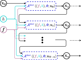
Figure 3: $T$ consecutive iterations using the R2N2 superstructure from Figure 2 compute a sequence $\left(\mathbf{x}_{1},\ldots,\mathbf{x}_{T}\right)$. The blue dashed cell delimits the iteration $\mathcal{A}^{iter}$ computed in a forward pass, i.e., one pass through the R2N2. The task-related inputs $h$ (cyan) and $\bm{f}$ (magenta) apply to each iteration. The initial guess $\mathbf{x}_{0}$ is an input only to the first iteration.

3.2 Relation to Krylov subspace methods

Numerical algorithms for solving (non-)linear equations as well as integrating sets of ordinary differential equations are traditionally based on local Taylor series expansions, and on the use of the first term (the Jacobian) – or even sometimes the second term (the Hessian) – in performing the numerical operations required to arrive at the next iteration. The solution of sets of linear equations resulting from sets of nonlinear equations, e.g., Newton iterations involving the solutions of linear equations, underpins a lot of today’s scientific computing. Due to the memory constraints of the early supercomputers (like the Cray 1), algorithms solving sets of linear equations through matrix-vector products and the construction of Krylov subspaces, e.g., GMRES, blossomed in the 1970s and 80s. Most importantly for us, these ideas evolved into matrix-free algorithms, like those embodied in matrix-free NK–GMRES. And through such ideas, algorithms evolved towards performing their tasks through intelligently planned recursive function evaluations. This leads to the premise that many scientific computations can be performed through systematic, recursive function evaluations (interspersed by brief low-dimensional tasks, like Gram-Schmidt orthogonalization, or least-squares solutions in low-dimensional subspaces) – and thus many algorithms essentially comprise of an intelligent (recursive) concatenation of function evaluations, enhanced by some ancillary computation. Thus, many traditional numerical algorithms are protocols for recursively recurrent function evaluations (plus ancillary computation). Both matrix-free NK–GMRES (for solving systems of nonlinear equations) and numerical initial-value problem solvers (of which RK is a notorious example) can be seen to naturally lead to R2N2 architectures. The analogy between an RK method and the R2N2 was already demonstrated in our previous work (Guo et al.,, 2022). Here, we show that the R2N2 also represents Krylov and NK subspace methods up to the ancillary computations.

3.2.1 Krylov subspace solvers

Krylov subspace solvers compute an approximate solution to linear systems of the form

$$\mathbf{A}\mathbf{x}=\mathbf{b},$$ (11)

where $\mathbf{A}\in\mathbb{R}^{m\times m}$ and $\mathbf{b}\in\mathbb{R}^{m}$, in an $n$-dimensional subspace $\mathcal{K}_{n}$, $n\leq m$, such that the norm of a residual $\mathbf{r}$, i.e.,

$$\left\|\mathbf{r}\right\|=\left\|\mathbf{A}\mathbf{x}-\mathbf{b}\right\|,$$

is minimized (Saad,, 2003). The Krylov subspace $\mathcal{K}_{n}$ is given by

$$\mathcal{K}_{n}(\mathbf{A},\mathbf{r}_{0})=\operatorname{\mathrm{span}}\left\{\mathbf{r}_{0},\mathbf{A}\mathbf{r}_{0},\mathbf{A}^{2}\mathbf{r}_{0},\ldots,\mathbf{A}^{n-1}\mathbf{r}_{0}\right\},$$ (12)

and is fully determined by $\mathbf{A}$ and the initial residual $\mathbf{r}_{0}$. In absence of prior knowledge, $\mathbf{r}_{0}$ is usually computed by choosing $\mathbf{x}_{0}=\mathbf{0}$, i.e., $\mathbf{r}_{0}=-\mathbf{b}$. The remaining Krylov vectors spanning the subspace are obtained by recurrent left-side multiplication of $\mathbf{r}_{0}$ with $\mathbf{A}$. Finally, the approximate solution follows as

$$\overline{\mathbf{x}}=\mathbf{x}_{0}+\mathbf{q}^{\star},$$ (13)

$$\mathbf{q}^{\star}\in\arg\operatorname{min}_{\mathbf{q}\in\mathcal{K}_{n}}\left\|\mathbf{A}\left(\mathbf{x}_{0}+\mathbf{q}\right)-\mathbf{b}\right\|.$$ (14)

$\mathbf{q}^{\star}$ can be expressed as a linear combination of the vectors spanning the subspace $\mathcal{K}_{n}$, i.e,

$$\mathbf{q}^{\star}=\mathbf{V}_{n}\bm{\upbeta},$$ (15)

where $\mathbf{V}_{n}$ is an $n\times n$ matrix that contains the members of $\mathcal{K}_{n}$ as columns and $\bm{\upbeta}\in\mathbb{R}^{n}$ is a vector of coefficients found by solving Problem (14). Contemporary Krylov methods like GMRES (Saad and Schultz,, 1986) orthonormalize the basis of $\mathcal{K}_{n}(\mathbf{A},\mathbf{r}_{0})$. This operation requires additional computation but enables explicit residual minimization.

Instead of solving Equation (14), the R2N2 superstructure approximates the solutions generated by the Krylov method, Equations (12) – (15), as follows. We set $\bm{f}(\mathbf{x})\vcentcolon=\mathbf{A}\mathbf{x}-\mathbf{b}$ such that the initial function evaluation returns $\mathbf{v}_{0}=\bm{f}(\mathbf{0})=\mathbf{r}_{0}=-\mathbf{b}$. Due to the nature of the layer modules $\bm{N}_{j}$, Equation (9), all layers after the initial layer will return outputs $\mathbf{v}_{j}$ that are in the span of $\left\{\mathbf{r}_{0},\mathbf{A}\mathbf{r}_{0},\ldots,\mathbf{A}^{j-1}\mathbf{r}_{0}\right\}$ such that the subspace generated by the R2N2 coincides with the Krylov subspace, Equation (12). The output module of the R2N2, Equation (10), learns a fixed linear combination of these $\mathbf{v}_{j}$ through its parameters $\bm{\uptheta}_{n}$. By identifying these $\bm{\uptheta}_{n}$ as $\bm{\upbeta}$, $\mathbf{x}_{k}$ as $\mathbf{x}_{0}$ and $h=1$, one forward pass through the R2N2 can, in principle, imitate one outer iteration of the Krylov subspace method for a single problem instance $\left(\mathbf{A},\mathbf{b}\right)$.

On the other hand, one pass through the R2N2 is cheaper than an iteration of a Krylov method, since the R2N2 does not perform the orthonormalization and explicit residual minimization. Both methods require $n-1$ matrix-vector products to build the $n$-dimensional subspace, given that $\mathbf{r}_{0}$ is obtained for free. Finally, we point out that some Krylov-based solvers, e.g., GMRES, can be iteratively restarted to compute a better approximation to a solution of a linear system (Saad and Schultz,, 1986). This restarting procedure is naturally represented by recurrent passes through the R2N2, i.e., a restart corresponds to updating the iterate from $\mathbf{x}_{k}$ to $\mathbf{x}_{k+1}$.

3.2.2 Newton-Krylov solvers

Newton-Krylov solvers essentially approximate Newton iterations for the solution of a nonlinear equation system $\bm{f}(\mathbf{x})=\mathbf{0}$, $\bm{f}\vcentcolon\mathbb{R}^{m}\rightarrow\mathbb{R}^{m}$, where the linear subproblem that arises in each Newton iteration is addressed using a Krylov subspace method (Kelley,, 1995, 2003; Knoll and Keyes,, 2004). The $k$-th linear subproblem requires solving

$$\mathbf{J}(\mathbf{x}_{k})\Delta\mathbf{x}_{k}=-\bm{f}(\mathbf{x}_{k}).$$

Therefore, the residual $\mathbf{r}_{0}$ of the linear solver corresponds to $\bm{f}(\mathbf{x}_{k})$ and the matrix $\mathbf{A}$ is substituted by the Jacobian of $\bm{f}$ at $\mathbf{x}_{k}$, $\mathbf{J}(\mathbf{x}_{k})\in\mathbb{R}^{m\times m}$. The corresponding $k$-th Krylov subspace then reads

$$\mathcal{K}_{n}^{(k)}\left(\mathbf{J}(\mathbf{x}_{k}),\bm{f}(\mathbf{x}_{k})\right)=\operatorname{\mathrm{span}}\left\{\mathbf{v}_{0},\ldots,\mathbf{v}_{n-1},\right\},$$ (16)

$$\mathbf{v}_{j}=\mathbf{J}(\mathbf{x}_{k})^{j}\bm{f}(\mathbf{x}_{k})\quad\forall\,j\in\{0,\ldots,n-1\}.$$

In the practical use-case of Newton-Krylov methods, $\mathbf{J}(\mathbf{x}_{k})$ is not computed explicitly. Instead, matrix-vector products $\mathbf{J}(\mathbf{x}_{k})\mathbf{z}$, where $\mathbf{z}\in\mathbb{R}^{m}$ is a vector, are approximated using a directional derivative of $\bm{f}$ at $\mathbf{x}_{k}$ (Kelley,, 2003), i.e.,

$$\mathbf{J}(\mathbf{x}_{k})\mathbf{z}\approx\frac{\bm{f}(\mathbf{x}_{k}+\epsilon\mathbf{z})-\bm{f}(\mathbf{x}_{k})}{\epsilon},$$

where $\epsilon$ is a small value in the order of $10^{-8}$. The RHS corresponds to forward-differencing, which is shown to lie within the R2N2 superstructure in the supplementary material (SM1). Typically, multiple iterates $\mathbf{x}_{k}$ have to be computed to sufficiently approximate a solution of $\bm{f}(\mathbf{x})=\mathbf{0}$. Such iterative behavior can be reproduced by performing multiple recurrent passes through the R2N2. Since $\mathbf{J}(\mathbf{x}_{k})$ is always computed with the current iterate $\mathbf{x}_{k}$, each pass through the R2N2 necessarily corresponds to a new Newton iteration if the remaining identities noted in the previous section, Section 3.2.1, on linear Krylov solvers are applied again. Consequently, the limited expressivity due to $\bm{\uptheta}_{n}$ as opposed to the minimization in a Krylov method is inherited, too.

3.3 Training the R2N2 superstructure

Training the R2N2 superstructure implies solving Problem (4) for the trainable parameters $\bm{\uptheta}$. The input data for each problem class is sampled from a distribution representing a set of problem instances, the solutions to which are the training targets. In the following, we indicate data samples by an additional subscript $i=1,\ldots,N$, where $N$ is the total number of samples, i.e., $\mathbf{x}_{i,k}$ refers to the $i$-th sample after the $k$-th iteration. The output of the $k$-th pass through an R2N2 is the iterate denoted by $\hat{\mathbf{x}}_{i,k+1}$. As a loss function we use a weighted version of the mean squared error (MSE) between $\hat{\mathbf{x}}_{i,k}$ and $\mathbf{x}_{i,k}^{target}$ or the corresponding residual $\Pi\left(\hat{\mathbf{x}}_{i,k},F_{i}\right)$, summed over all iterations, i.e.,

$$MSE_{x}=\frac{1}{N}\sum_{k=1}^{T}\sum_{i=1}^{N}w_{i,k}{\left\|\hat{\mathbf{x}}_{i,k}-\mathbf{x}^{target}_{i,k}\right\|_{2}}^{2},$$ (17a)

$$MSE_{\Pi}=\frac{1}{N}\sum_{k=1}^{T}\sum_{i=1}^{N}w_{i,k}{\Pi(\hat{\mathbf{x}}_{i,k},F_{i})}^{2},$$ (17b)

where $w_{i,k}$ are the weights belonging to the $i$-th sample in the $k$-th iteration. Whether we utilize Equation (17a) or Equation (17b) is problem-specific. For instance, for equation solvers, we can make use of $\bm{f}(\mathbf{x}^{\star}_{i}):=\mathbf{0}$ to compute the residual for Equation (17b) from $\bm{f}(\mathbf{x}_{i,k+1})$. For integrators on the other hand, we can sample training targets $\mathbf{x}_{i,k+1}^{target}$ from the trajectory computed by some high-order integrator or, if available, use an analytic solution to generate target data. We do not use any regularizers for training the R2N2 in this work.

3.4 Implementation

We implemented the R2N2 superstructure in PyTorch (version $1.8.0$) (Paszke et al.,, 2019). We trained on an Intel i7-9700K CPU using Adam (Kingma and Ba,, 2015) for $25,000$ epochs with the default learning rate of $0.001$ or L-BFGS (Liu and Nocedal,, 1989) for $5,000$ epochs with a learning rate of $0.01$. Note that L-BFGS is commonly used to fine-tune networks with comparable architecture as ours that were pretrained with Adam, e.g., by Zhao and Mau, (2020), suggesting that L-BFGS can improve the training result. A detailed assessment of the capability of different optimizers and strategies to train the R2N2 superstructure is beyond the scope of this work.

4 Numerical experiments

In this section, we demonstrate the ability of the R2N2 superstructure to learn efficient iterations for both equation solvers and integrators. Section 4.2 and Section 4.3 will show that computational benefits of solvers trained for a specific problem class start to arise in solving nonlinear problems with such algorithms. In particular, Section 4.2 demonstrates the extended applicability of the RK-NN introduced in Guo et al., (2022) to nonlinear equation systems. We start here, however, with linear systems of equations in Section 4.1, not because of the computational benefits achievable, but because the comparison between the R2N2 and GMRES (as a matrix-free linear algebra solver) facilitates initial insight into the functionality of the R2N2 when learning iterative solvers for equation systems.

In all experiments that follow, the R2N2 and the classical method it is compared to are allowed the same number of function evaluations per iteration. Thus, for equation solvers, the R2N2 requires less overall operations per iteration, c.f. Section 3.2, and for integrators, the amount of overall operations per iteration will be identical. We have consistently used $70\%$ of the generated data for training and an independent sample of $30\%$ for the test results that are presented in the following.

4.1 Solving linear equation systems

First, we study the solution of linear equations, see Equation (11). For the illustrative experiments we consider examples where a single task is given by $F_{i}=\left(\mathbf{A}_{1},\mathbf{b}_{i}\right)$ with $\mathbf{A}_{1}\in\mathbb{R}^{m\times m}$, $\mathbf{b}_{i}\in\mathbb{R}^{m}$, $\mathbf{x}\in\mathbb{R}^{m}$ and $m=5$. $\mathbf{A}_{1}$ is a fixed, randomly-generated symmetric positive definite matrix overlaid with an additional boost to its diagonal entries to influence its spectrum. Right-hand sides (RHS) $\mathbf{b}_{i}$ are sampled uniformly around a fixed randomly-chosen mean. See supplementary material (SM2) for details. As training input we use the data set of tasks $\{F_{i}\}=\{(\mathbf{A}_{1},\mathbf{b}_{i})\}$ and always select $\mathbf{x}_{0}=\mathbf{0}$ as the initial point. Therefore, the resulting $n$-dimensional Krylov subspace is always spanned by $\left\{\mathbf{b}_{i},\mathbf{A}_{1}\mathbf{b}_{i},\ldots,\mathbf{A}_{1}^{n-1}\mathbf{b}_{i}\right\}$. When injecting the input data to the R2N2, we resort to $\bm{f}(\mathbf{x}_{i})\vcentcolon=\mathbf{A}_{1}\mathbf{x}_{i}-\mathbf{b}_{i}$. We use $\bm{f}\left(\mathbf{x}_{i,k+1}^{t}\right)=\mathbf{0}$ as training targets for all samples $i$ and all steps $k$. Therefore, the training loss at a step $k$, derived from Equation (17b), becomes

$$MSE_{f,k}=\sum_{k=1}^{T}w_{k}\sum_{i=1}^{N}\left(\mathbf{A}_{1}\hat{\mathbf{x}}_{i,k}-\mathbf{b}_{i}\right)^{2},$$ (18)

where $w_{k}$ becomes relevant when training over multiple iterations, $T>1$, and is tuned by hand.

To evaluate the performance of the R2N2, we compute the reduction of the norm of the residual that was achieved after $k$ iterations through the R2N2, i.e.,

$$\Delta\mathbf{r}_{i,k}=\left\|\mathbf{b}_{i}\right\|-\left\|\mathbf{A}_{1}\hat{\mathbf{x}}_{i,k}-\mathbf{b}_{i}\right\|.$$ (19)

For the results that follow, we compare the R2N2 to the SciPy implementation of the solver GMRES (Saad and Schultz,, 1986; Virtanen et al.,, 2020). GMRES is set to use the same number of inner iterations, i.e., function evaluations as the R2N2. Considering the restarted version of GMRES, GMRES(r), a forward pass through the R2N2 represents one outer iteration (Saad and Schultz,, 1986). We evaluate the reduction in residual norm divided by the one achieved using GMRES, i.e., $\frac{\left\|\Delta\mathbf{r}_{1,i}\right\|_{R2N2}}{\left\|\Delta\mathbf{r}_{1,i}\right\|_{GMRES}}$, with the subscripts ‘R2N2’ indicating the R2N2 and ‘GMRES’ indicating the solver GMRES.

The training result of this first experiment is shown in Figure 4(a). Notably, the performance of the R2N2 is upper-bounded by the performance of GMRES, as GMRES minimizes the residual in the subspace spanned by the Krylov vectors. Given that this subspace is invariant with respect to the operations that can be learned by the layers of the R2N2 for the linear problem instances, the R2N2 cannot improve on the performance of GMRES in this first case study.

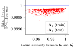
(a) Training and testing with only $\mathbf{A}_{1}$. Light dots show training samples.

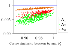
(b) Testing on instances featuring $\mathbf{A}_{1}$, $\mathbf{A}_{2}$ and $\mathbf{A}_{3}$.

Figure 4: Relative performance of R2N2 vs GMRES with $n=4$ inner iterations for problem instances of Problem (11). Each dot indicates a different RHS $\mathbf{b}_{i}$. The blue lines indicate the baseline achieved by GMRES. Subscripts ‘R2N2’ and ‘GMRES’ stand for the R2N2 and GMRES, respectively. Each method returns a step in a $4$-dimensional subspace, which is generated via $3$ function evaluations. The residual reduction is computed using Equation (19) with the respective $\mathbf{A}_{j}$ for $j\in\{1,2,3\}$. The scales in a) and b) are different. By $\mathbf{b}_{j}^{\star}$ we denote the sample for which the relative performance of R2N2 is maximized for each case. In (a), the training data set features only problems with $\mathbf{A}_{1}$, while in (b), three different matrices are used.

The experiment with a fixed $\mathbf{A}_{1}$ was chosen to illustrate this upper bound of the R2N2 and does not yield a proper problem distribution for the training set – with $\mathbf{A}_{1}$ fixed, only a mapping from $\mathbf{b}_{i}$ to $\mathbf{x}_{i}^{\star}$ needs to be learned. Thus, we now draw two additional matrices, $\mathbf{A}_{2},\mathbf{A}_{3}\in\mathbb{R}^{m\times m}$ from the distribution (see (SM2)). Through the addition of $\mathbf{A}_{2}$ and $\mathbf{A}_{3}$, the performance, i.e., the adaptation, of the resulting R2N2 on problem instances formed with either of the three matrices is decreased compared to the previous case (see Figure 4(b)).

Next, we study the performance of the R2N2 over multiple iterations together with the extrapolation capabilities of the R2N2. Here, the R2N2 is compared with the restarted version of GMRES, GMRES(r), where each iteration uses the output of the previous iteration as an initial value. We train the R2N2 to minimize loss after three outer iterations, given by Equation (18). We set $w_{k}=4^{k}$, which was found to yield decent results. The training dataset is again generated from the random draw of samples of $\mathbf{b}_{i}$ combined with the three matrices $\mathbf{A}_{1}$, $\mathbf{A}_{2}$, and $\mathbf{A}_{3}$. The solid red line in Figure 5 shows the convergence of the R2N2 by plotting the average residual of the test set for $\mathbf{A}_{1}$ only (for clarity). The R2N2 reduces the residual over all consecutive outer iterations, i.e., even beyond the third outer iteration, which indicates a first type of successful extrapolation of the R2N2: Iterates $\mathbf{x}_{k}$ for $k>3$ have not been contained by the training input distribution, yet the R2N2 iterations progress towards the solution of the problem beyond that point. Related to this extrapolation on RHS given by iterates $\mathbf{x}_{k}$ is the orange dash-dotted line that examines the R2N2 on uniform random RHSs $\mathbf{b}_{i}$, normalized to the length of the test set samples. The R2N2 is shown to converge to a solution for all of these RHSs, i.e., the convergence is due to a property of the R2N2 and $\mathbf{A}_{1}$. We analyze this further in supplementary material (SM4).

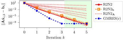
Figure 5: Convergence of the R2N2 vs GMRES(r) for solving (11) for multiple samples of $\mathbf{b}_{i}$. The lines connect the sample mean at each (outer) iteration $k$. Both solvers use $n=4$ inner iterations. The R2N2 was trained on $T=3$ outer iterations, using Equation (18) with $w_{k}=4^{k}$ as a loss, and then applied over $5$ iterations. Iterations within the shaded square area, $k>3$, have not been seen in training and indicate one type of extrapolation. The orange-squared line ‘R2N2_b’ shows extrapolation in the RHS, and the dotted lines ‘R2N2_A’ show extrapolations in matrices $\mathbf{A}$ (see (SM3.1) for details).

Finally, we analyze two additional types of extrapolation applied to $\mathbf{A}_{1}$: i) raising the noise level of its random component by up to a factor of $7$, ii) reducing or increasing the induced spectrum in $\mathbf{A}_{1}$, respectively. See supplementary material (SM3.1) for details. Trajectories for the resulting test matrices – again combined with the initial RHS samples of $\mathbf{b}_{i}$ – are plotted as light-red dotted lines in Figure 5. The results demonstrate that the R2N2 learns a solver adapted to a problem data set, and, further, that the R2N2 extrapolates reasonably well beyond that data set, with a performance decrease as $\mathbf{A}$ becomes more different from the training distribution. The extrapolation experiments are presented in more detail – including some failure cases – in (SM3.1). We also show that vanilla neural networks (NNs) of comparable size cannot learn a solver like the R2N2 (SM3.2), and that a R2N2 modified to predict solutions does better than the NNs in this task too (SM3.3).

As a final example, we demonstrate that the R2N2 can also be applied to an embedding of the problem class. We generate a random $15$-dimensional orthonormal matrix $\mathbf{Q}$ from the Haar distribution via SciPy (Virtanen et al.,, 2020; Mezzadri,, 2006), and consider the problem class with instances

$$\mathbf{Q}\mathbf{A}_{1}\mathbf{Q}^{T}\mathbf{x}=\mathbf{Q}\mathbf{b}_{i},$$ (20)

where by abuse of notation $\mathbf{A}_{1}$ and $\mathbf{b}_{i}$ are made $15$-dimensional by zero-padding the new dimensions. The convergence of the residual of this embedded problem is shown in Figure 6.

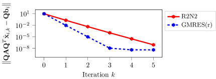
Figure 6: Convergence of the R2N2 applied to the embedded problem (20). The R2N2 was trained on samples from the original problem (11) (same R2N2 as the one used in Figure 5). Both solvers again use $n=4$ inner iterations. The lines connect the sample mean at each (outer) iteration $k$.

Evidently, as an adapted solver, the R2N2 is also applicable to this embedding of the problem class it was trained on. By inspecting the embedding, we see that the resulting subspace vectors are also rotated by $\mathbf{Q}$, i.e.,

$$\mathcal{K}_{n}\left(\mathbf{Q}\mathbf{A}\mathbf{Q}^{T},\mathbf{Q}\mathbf{b}\right)=\left(\mathbf{Q}\mathbf{b},\mathbf{Q}\mathbf{A}\mathbf{b},\ldots,\mathbf{Q}\mathbf{A}^{n-1}\mathbf{b}\right),$$

as the $\mathbf{Q}^{T}\mathbf{Q}$ in the inner of the matrix-vector products cancels out each time.

4.2 Solving nonlinear equation systems

As an illustrative nonlinear equation system, we consider Chandrasekhar’s $H$-function in conservative form, an example that was extensively used in Kelley’s book on Newton-Krylov solvers (Kelley,, 2003). The discretized form of this equation reads

$$\left(\bm{f}(\mathbf{x})\right)_{j}=\mathbf{x}_{j}-\left(1-(\mathbf{A}_{c}\mathbf{x})_{j}\right)^{-1},$$ (21)

for $j=1,\ldots,m$ with the entries of parametric matrix $\mathbf{A}_{c}\in\mathbb{R}^{m\times m}$ defined by

$$A_{c,j\iota}=\frac{c\mu_{j}}{2m\left(\mu_{j}+\mu_{\iota}\right)},$$

with $\mu_{\iota}=\frac{(\iota-\frac{1}{2})}{m}$ and $\iota=1,\ldots,m$ also indexing the discretization points. The derivation of the equations is given in supplementary material (SM2). We combine problems with $m=10$ and $m=20$ discretization points and $c\in\left\{0.875,0.905,0.935\right\}$ to span a training set. For all of these problems, we sample initial values $\mathbf{x}_{0,i}$ from a normal distribution with mean $\mathbbm{1}^{(m)}$, where $\mathbbm{1}^{(m)}$ is an $m$-dimensional vector of ones, and variance $0.2\cdot\mathbbm{1}^{(m)}$. We again use (18) as a loss function, where targets are $\bm{f}\left(\mathbf{x}_{k+1,i}^{t}\right)=0$ for all samples $i$ and iterations $k$. The SciPy implementation of Kelley’s Newton-Krylov GMRES (NK-GMRES) serves as a benchmark (Virtanen et al.,, 2020; Kelley,, 2003).

We evaluate the performance after $k$ nonlinear iterations by the reduction in the norm of the residual:

$$\Delta\mathbf{r}_{k}=\left\|\bm{f}(\mathbf{x}_{0})\right\|-\left\|\bm{f}(\mathbf{x}_{k})\right\|.$$ (22)

Figure 7 showcases the performance of the R2N2 on individual samples after training for $2$ nonlinear iterations. The R2N2 is able to achieve more progress within these first two iterations than NK-GMRES even though it does not explicitly perform the minimization in the Krylov subspace to compute the step. The advantage in performance is maintained over a range of values for coefficient $c$ in $\mathbf{A}_{c}$ both within the training range (red markers) and outside of the training range (light green). We therefore deduce that the R2N2 has learned to construct a subspace that contains more of the true solution for a specific problem class than the subspace formed by NK-GMRES. This is possible because the subspace $\mathcal{K}_{n}\left(\mathbf{J}(\mathbf{x}_{k}),-\bm{f}(\mathbf{x}_{k})\right)$, Equation (16), used in the $k$-th iteration depends not only on $\left(\bm{f},\mathbf{x}_{k}\right)$ but also on the trainable parameters $\bm{\uptheta}_{j}$ in the $\bm{N}_{j}$ modules of the R2N2, cf. Equation (7b). Finally, we observed no notable difference between problem samples with $m=10$ and $m=20$.

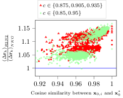
(a) After $k=1$ nonlinear iterations.

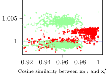
(b) After $k=2$ nonlinear iterations.

Figure 7: Relative performance of R2N2 vs NK-GMRES using $n=3$ inner iterations and one (a) or two (b) outer iterations on Problem (21) with various coefficients $c$ and various initial guesses $\mathbf{x}_{0,i}$. Note the differences in scales between the two subfigures. Instances where $c$ is extrapolated outside of the training range are plotted in light green. The residuals are computed using Equation (22) with subscripts ‘R2N2’ and ’NKG’ for the R2N2 and the NK-GMRES solver, respectively. $\mathbf{x}_{0}^{\star}$ refers to the sample for which the relative performance of R2N2 is best in the respective experiment.

We applied the R2N2 from Figure 7 for a total of $7$ nonlinear iterations, see Figure 8. The advantage of the R2N2 over NK-GMRES vanishes for $3$ and more nonlinear iterations, but the R2N2 does still converge to an approximate solution when applied iteratively. Note, however, that this promising finding does not guarantee that the R2N2 can be trained to converge to a solution of arbitrary nonlinear equation systems. Furthermore, Figure 8 shows extrapolation to problems with $m=100$. Similar to the case in the previous subsection, the R2N2 is agnostic of the problem dimension, which in this case allows generalization across various discretizations of the problem. Thus, overall the R2N2 is applicable to solving instances of Equation (21) without explicit access to either of its generative properties, i.e., $c$ and $m$, something an unstructured neural network trained on problem data was found to be incapable of, cf. (SM2).

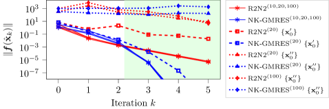
Figure 8: Convergence of the R2N2 (red) vs NK-GMRES (blue) for $8$ nonlinear iterations of solving (21). Both solvers use $3$ inner iterations. The R2N2 used herein coincides with the one shown in Figure 7(b), i.e., it was trained only on the first $2$ nonlinear iterations. The shaded area $k>2$ denotes performing more iterations than were used for training. The superscripts indicate the set of problem dimensions $m$ used. Performance for samples of $\{\mathbf{x}_{0}\}$ from the training range are shown by solid lines. Dashed lines use initial samples $\{\mathbf{x}^{\prime}_{0}\}$ with 10-fold noise around $\mathbbm{1}^{(m)}$, whereas dotted lines use initial samples $\{\mathbf{x}^{\prime\prime}_{0}\}$ centered at $5\cdot\mathbbm{1}^{(m)}$.

Finally, we studied extrapolation for different initial guesses. The test set denoted by $\{\mathbf{x}^{\prime}_{0}\}$ is generated with 10-fold variance compared to the training set, whereas the test set denoted $\{\mathbf{x}^{\prime\prime}_{0}\}$ consists of initial guesses centered around a different vector, here $5\cdot\mathbbm{1}^{m}$s. For the latter, the R2N2 shows some convergence, also continuing over further iterations that were not plotted herein. After 15 iterations, all test samples except for a couple (that are still converging) have reached a tolerance of $1e-8$. NK-GMRES, on the other hand, produces more outliers: after 15 iterations, only $63.2\leavevmode\nobreak\ \%$ of samples have converged. This number is increased to $76.7\leavevmode\nobreak\ \%$ after 20 iterations, $98\leavevmode\nobreak\ \%$ after 50 iterations and $99.4\leavevmode\nobreak\ \%$ after 75 iterations. That is, the mean curves are dominated by the instances that are slow to converge. This distinct difference in performance between the R2N2 and NK-GMES merits further study.

4.3 Solving initial-value problems

Finally, we study the solution of initial-value problems with the known RHS $\bm{f}$, i.e., Problem (3). We covered learning integrators thoroughly in our previous work (Guo et al.,, 2022) where we employed a Taylor series-based regularization to promote certain orders of convergence as property of the RK-NN. We now demonstrate that RK-NN integrators that outperform classical RK integrators can also be learned without special regularizers and, as a further extension of our previous work, that the RK-NN integrators work over multiple timesteps. All RK-NNs in this section are trained from the R2N2 superstructure and we thus name them R2N2 in the remainder of the section.

We reiterate the van der Pol oscillator from our previous work, i.e.,

$$\dot{x}_{(1)}(t) =x_{(2)}(t),$$ (23a)

$$\dot{x}_{(2)}(t) =a\left(1-x_{(1)}^{2}(t)\right)x_{(2)}(t)-x_{(1)}(t),$$ (23b)

with $\mathbf{x}=\left(x_{(1)},x_{(2)}\right)$. For data generation, we sample coefficients $a\sim\mathcal{U}(1.35,1.65)$, initial values $x_{(1)}(t=t_{0})\sim\mathcal{U}(-4,-3)$ and $x_{(2)}(t=t_{0})\sim\mathcal{U}(0,2)$ and timesteps $h\in\left[0.01,0.1\right]$ equidistantly Note that $\mathbf{x}(t=t_{0})$ and $h$ are contained in the problem parameters $\mathbf{p}$. For Problem (3), we use them directly as the inputs $\mathbf{x}_{k}$ and $h$ of the R2N2, cf. Figure 2. We generate target data (that also servers as ground truth) for the timesteps $h$ using SciPy’s odeint (Virtanen et al.,, 2020) with error tolerance set to $10^{-8}$. Training loss is calculated by the following specification of Equation (17a):

$$MSE_{x}=\sum_{k=1}^{T}\sum_{i=1}^{N}\frac{\left(\hat{\mathbf{x}}_{i,k}-\mathbf{x}_{i,k}^{t}\right)^{2}}{h_{i}^{p}}.$$

The losses are summed over $T$ integration steps of a trajectory with the timestep $h$, i.e., at times $t_{0}+h,t_{0}+2h,\ldots,t_{0}+Th$. Further, the denominator of the loss terms allows weighting samples based on the timestep of a specific sample, $h_{i}$, and, in particular, weighting according to an expected convergence order $p$. We set $p=n$ for the results in Section 4.3, where $n$ is the number of layers of the RK-NN. The function evaluations in the R2N2 directly evaluate the RHS of Equation (23). One pass through the R2N2 therefore resembles one step of a RK method.

To assess the performance of the learned integrators, we compare the R2N2 instantiated with $n$ layers to classical RK methods of $n$ stages, denoted by RK-$n$. The training data contains samples with varying coefficients $a_{i}$, timesteps $h_{i}$ and initial values $\mathbf{x}_{i}(t=0)$. The error for either integrator is evaluated against a ground truth approximated by odeint and denoted $\mathbf{x}_{k}^{t}$. Results using $n=3$ on the van der Pol oscillator, Equation (23), are shown in Figure 9.

(a) The R2N2 error after one step is shown.

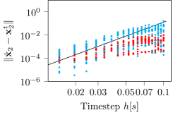
(b) The R2N2 error after two steps is shown.

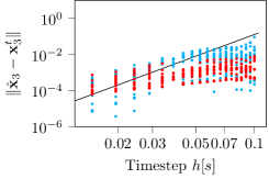
(c) The R2N2 error after three steps is shown.

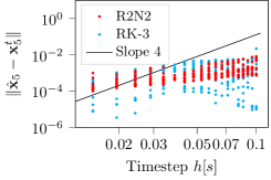
(d) The R2N2 error after five steps is shown.

Figure 9: Performance of R2N2 vs RK-$3$ integrating the van der Pol oscillator equations, Equation (23), with varying coefficients $a$, stepsizes $h_{i}$ and initial conditions $\mathbf{x}_{0,i}$. The figures show the same R2N2, trained on one timestep, and evaluated after one (a), two (b), three (c) and five timesteps (d), respectively. The slope of 4 is added to indicate the nominal local truncation error of RK-3.

In Figure 9(a)–9(d), we show results for training on $T=1$ step of integration and evaluating on $T=1$, $T=2$, $T=3$, and $T=5$ steps, respectively, i.e., for $k>1$, the iterates $\mathbf{x}_{k}$ that go into the R2N2 as inputs lie outside of its training range. We thus test for, and verify, some limited generalization. Over the first three timesteps, the R2N2 integrates the van der Pol oscillator equations more accurately than RK-$3$. We want to stress here that the classical RK method uses fixed coefficients for the computation of stage values and for the computation of the step itself. Therefore, the R2N2 can improve over the classical RK with regards to both of these computational steps. Evidently, we are able to learn coefficients $\bm{\uptheta}_{j}$ in the stages $\bm{N}_{j}$ and $\bm{\uptheta}_{n}$ for the output $\bm{N}_{n}$ that lead to a better approximation of the integral for problems from the training distribution, including limited generalization, than the RK method does.

Overall, we find that the accuracy of the R2N2 gradually decreases over the number of timesteps such that the R2N2 is not more accurate than RK-$3$ after the $5$-th iteration anymore. The trend observed in Figure 9(a)–9(d), although less pronounced, is consistent with the behavior of the R2N2 over multiple iterations of equation solving.

5 Conclusion

This work proposes an alternative, augmented perspective for the use of the RK-NN, a recurrent neural network templated on RK integrators, as a recursively recurrent superstructure for a wider class of iterative numerical algorithms. The R2N2 superstructure embeds function evaluations inside its layers and feeds the output to all successive layers via forward skip connections and linear combinations. The embedding of function calls into the architecture disentangles the algorithm to be learned from the function it acts on. We have shown that the R2N2 superstructure provides an inductive bias towards iterative algorithms based on recurrent function evaluation, e.g., the well-established Krylov subspace solvers and RK methods. Our numerical experiments demonstrate that, thus, the R2N2 superstructure can mimic steps of Krylov, Newton-Krylov and RK algorithms, respectively.

In particular, when learning a single step of linear equation solvers (Section 4.1), the performance of the R2N2 is bounded by that of the benchmark GMRES. This is consequential considering that the subspaces generated by the two approaches are equal but GMRES further minimizes the residual in this subspace, whereas the R2N2 learns a linear combination that can coincide with the minimizer, cf. Equation (14), for at most a single problem instance. In contrast, a nonlinear equation solver (Section 4.2) can improve upon iterations performed by NK-GMRES, because in this case the R2N2 can learn to construct subspaces in which the residual is reduced more strongly than by NK-GMRES. Applying the R2N2 for multiple outer iterations resembles a restarted iterative solver for linear problems or a Newton-Krylov method for nonlinear problems, respectively. We have empirically demonstrated the ability of the R2N2 to converge to solutions of linear and nonlinear equation solving problems, however, we cannot guarantee the convergence of trained solvers for arbitrary problems. The R2N2 is also capable of extrapolation to similar problems as the ones seen during training. This includes not only extensions to the range of problem parameters but also embedding in higher dimensions or finer discretization. Finally, we have revisited our previous work about learning RK integrators (Guo et al.,, 2022) by demonstrating successful integration over multiple timesteps (Section 4.3). Our results suggest that the advantage of the R2N2 or RK-NN, respectively, over a classical RK method cannot be sustained over longer time horizons of integration.

In summary, iterative algorithms trained within the R2N2 superstructure can, when possible, find a subspace in which the residual can be reduced more than by their classical counterparts, given the same number of function evaluations.

6 Future research directions

6.1 Application to other computational problems

For further application, the compatibility of the R2N2 superstructure with other problem classes that comply with the general form of Problem (1) and that are solved with iterative algorithms, e.g., eigenvalue computation, PCA decomposition (Gemp et al.,, 2021), or computation of Neumann series (Liao et al.,, 2018), could be assessed. Moreover, besides learning an algorithm as a neural network architecture that maps from a set of problems to their solutions, the superstructure proposed in this work can also be deployed in the inverse setting, i.e., to identify a problem or function under the action of the known algorithm given input/output data. This was the original motivation in Rico-Martinez et al., (1995), leading to nonlinear system identification, that can be analyzed using inverse backward error analysis (Zhu et al.,, 2020, 2023).

6.2 Extension of the superstructure

Other, more intricate algorithms can be represented by the proposed superstructure if its architecture is extended with additional trainable modules. For instance, general linear methods for integration (see Butcher, (2016)) can be captured by the superstructure if not just the final output is subject to recurrence, but the layer outputs $\mathbf{v}_{j}$ are too (cf. with Figure 2). Moreover, a preconditioner (see Section 8 of Saad and Van Der Vorst, (2000)) can be inserted inside the layers of the superstructure: for instance, a cheap, approximate model of $\bm{f}$ can be used to to effectively build such a preconditioner (Qiao et al.,, 2006). Finally, non-differentiable operations that are part of most algorithms, e.g., the checking of an error tolerance, can be included via smoothed relaxations (Ying et al.,, 2018; Tang et al.,, 2020).

6.3 Neural architecture search

Larger architectures will eventually call for superstructure optimization to yield parsimonious algorithms, i.e., determining the optimal (sub-)structure for a given set of problem instances together with the optimized parameters. This challenge can be formulated as a mixed-integer nonlinear program (MINLP). Presently, these problems are addressed by heuristic methods, referred to as neural architecture search (NAS, Elsken et al., 2019b ; Hospedales et al., (2021)), that are relatively efficient in finding good architectures. For the superstructure, three types of NAS methods appear suited: i) structured search spaces to exploit modularity, e.g., (Liu et al.,, 2017), (Zoph et al.,, 2018), (Negrinho et al.,, 2019) and (Schrodi et al.,, 2022), ii) adaptively growing search spaces for refining the architecture, e.g., (Cortes et al.,, 2017), (Elsken et al., 2019a, ) and (Schiessler et al.,, 2021), and iii) differentiable architecture search, e.g., (Liu et al.,, 2019) (Li et al., 2021a, ). Sparsity promoting training techniques like pruning typically address dense, fully-connected layers and, therefore, are expected to provide little use in the current architecture. Similar reasoning applies to generic regularizers like $\mathcal{L}_{2}$ regularization. On the other hand, tailored regularizers such as physics-informed losses or the regularizer we proposed in Guo et al., (2022) can prove useful to promote specific algorithmic properties.

More traditional MINLP solvers like those used for superstructure optimization of process systems (Grossmann,, 2002; Burre et al.,, 2022) exhibit certain advantages over NAS methods. They explicitly deal with integer variables allowing sophisticated use of discrete choices e.g., for mutually exclusive architecture choices. Moreover, MINLPs can be solved deterministically to guarantee finding a global solution, e.g., by a branch-and-bound algorithm (Belotti et al.,, 2013). Global solution of MINLPs involving the superstructure is challenging, since it requires neural network training subproblems to be solved globally. With future advances in computational hardware and algorithms this may become a viable approach. However, substantial effort is needed to utilize such MINLP solvers for the training tasks considered herein.

6.4 Implicit layers

An orthogonal approach for increasing the scope of the superstructure and capitalizing on its modularity is to endow only a subset of its modules or layers with trainable variables. The remaining modules that are not subject to meta-optimization can be implemented by so called implicit layers that implement their functionality, see, e.g., (Rajeswaran et al.,, 2019) and (Lorraine et al.,, 2020). In future work, we plan to emulate the residual minimization of Krylov solvers by substituting the output layer $\bm{N}_{n}$ of the superstructure with differentiable convex optimization layers (Amos and Kolter,, 2017; Agrawal et al.,, 2019). Then, only the optimal subspace generation, i.e., the parameters of the $\bm{N}_{j}$ modules, is left to learn, or the subspace generation is optimized with respect to consecutive minimization being performed in that subspace, respectively.

6.5 Dynamical systems perspective

A joint perspective on neural networks and dynamical systems has emerged recently, e.g., (E,, 2017), (Haber and Ruthotto,, 2017), and (Chang et al.,, 2017). Similarly, a connection between dynamical systems and continuous-time limits of iterative algorithms has been discussed in literature (Stuart and Humphries,, 1998; Chu,, 2008; Dietrich et al.,, 2020), especially for convex optimization (Su et al.,, 2014; Krichene et al.,, 2015; Wibisono et al.,, 2016). Researchers have applied numerical integration schemes to these continuous forms to recover discretized algorithms (Scieur et al.,, 2017; Betancourt et al.,, 2018; Zhang et al.,, 2018). Conversely, the underlying continuous-time dynamics of discrete algorithms encoded by the proposed R2N2 can be identified based on the iterates they produce, e.g., by their associated Koopman operators (Dietrich et al.,, 2020). These Koopman operators can then be analyzed to compare various algorithms and, even, to identify conjugacies between them (Redman et al.,, 2022).

Declaration of Competing Interest

We have no conflict of interest.

Bibliography

- Agrawal et al., (2019) Agrawal, A., Amos, B., Barratt, S. T., Boyd, S. P., Diamond, S., and Kolter, J. Z. (2019). Differentiable convex optimization layers. In Wallach, H. M., Larochelle, H., Beygelzimer, A., d’Alché-Buc, F., Fox, E. B., and Garnett, R., editors, Advances in Neural Information Processing Systems 32: Annual Conference on Neural Information Processing Systems 2019, NeurIPS 2019, December 8-14, 2019, Vancouver, BC, Canada, pages 9558–9570.
- Amos and Kolter, (2017) Amos, B. and Kolter, J. Z. (2017). Optnet: Differentiable optimization as a layer in neural networks. In Precup, D. and Teh, Y. W., editors, Proceedings of the 34th International Conference on Machine Learning, ICML 2017, Sydney, NSW, Australia, 6-11 August 2017, volume 70 of Proceedings of Machine Learning Research, pages 136–145. PMLR.
- Andrychowicz et al., (2016) Andrychowicz, M., Denil, M., Colmenarejo, S. G., Hoffman, M. W., Pfau, D., Schaul, T., and de Freitas, N. (2016). Learning to learn by gradient descent by gradient descent. In Lee, D. D., Sugiyama, M., von Luxburg, U., Guyon, I., and Garnett, R., editors, Advances in Neural Information Processing Systems 29: Annual Conference on Neural Information Processing Systems 2016, December 5-10, 2016, Barcelona, Spain, pages 3981–3989.
- Balcan, (2020) Balcan, M. (2020). Data-driven algorithm design. In Roughgarden, T., editor, Beyond the Worst-Case Analysis of Algorithms, pages 626–645. Cambridge University Press.
- Balcan et al., (2018) Balcan, M., Dick, T., Sandholm, T., and Vitercik, E. (2018). Learning to branch. In Dy, J. G. and Krause, A., editors, Proceedings of the 35th International Conference on Machine Learning, ICML 2018, Stockholmsmässan, Stockholm, Sweden, July 10-15, 2018, volume 80 of Proceedings of Machine Learning Research, pages 353–362. PMLR.
- Baxter, (2000) Baxter, J. (2000). A model of inductive bias learning. Journal of Artificial Intelligence Research, 12:149–198.
- Belotti et al., (2013) Belotti, P., Kirches, C., Leyffer, S., Linderoth, J., Luedtke, J., and Mahajan, A. (2013). Mixed-integer nonlinear optimization. Acta Numerica, 22:1–131.
- Betancourt et al., (2018) Betancourt, M., Jordan, M. I., and Wilson, A. C. (2018). On symplectic optimization. arXiv preprint arXiv:1802.03653.
- Burre et al., (2022) Burre, J., Bongartz, D., and Mitsos, A. (2022). Comparison of MINLP formulations for global superstructure optimization. Optimization and Engineering, pages 1–30.
- Butcher, (2016) Butcher, J. C. (2016). Numerical methods for ordinary differential equations. Wiley, Chichester, West Sussex, third edition edition.
- Chang et al., (2017) Chang, B., Meng, L., Haber, E., Tung, F., and Begert, D. (2017). Multi-level residual networks from dynamical systems view. arXiv preprint arXiv:1710.10348.
- Chen et al., (2018) Chen, T. Q., Rubanova, Y., Bettencourt, J., and Duvenaud, D. (2018). Neural ordinary differential equations. In Bengio, S., Wallach, H. M., Larochelle, H., Grauman, K., Cesa-Bianchi, N., and Garnett, R., editors, Advances in Neural Information Processing Systems 31: Annual Conference on Neural Information Processing Systems 2018, NeurIPS 2018, December 3-8, 2018, Montréal, Canada, pages 6572–6583.
- Chevalier et al., (2021) Chevalier, S., Stiasny, J., and Chatzivasileiadis, S. (2021). Contracting neural-newton solver. arXiv preprint arXiv:2106.02543.
- Chu, (2008) Chu, M. T. (2008). Linear algebra algorithms as dynamical systems. Acta Numerica, 17:1–86.
- Cortes et al., (2017) Cortes, C., Gonzalvo, X., Kuznetsov, V., Mohri, M., and Yang, S. (2017). Adanet: Adaptive structural learning of artificial neural networks. In International Conference on Machine Learning, pages 874–883. PMLR.
- Denevi et al., (2018) Denevi, G., Ciliberto, C., Stamos, D., and Pontil, M. (2018). Learning to learn around A common mean. In Bengio, S., Wallach, H. M., Larochelle, H., Grauman, K., Cesa-Bianchi, N., and Garnett, R., editors, Advances in Neural Information Processing Systems 31: Annual Conference on Neural Information Processing Systems 2018, NeurIPS 2018, December 3-8, 2018, Montréal, Canada, pages 10190–10200.
- Dietrich et al., (2020) Dietrich, F., Thiem, T. N., and Kevrekidis, I. G. (2020). On the Koopman operator of algorithms. SIAM Journal on Applied Dynamical Systems, 19(2):860–885.
- Dufera, (2021) Dufera, T. T. (2021). Deep neural network for system of ordinary differential equations: Vectorized algorithm and simulation. Machine Learning with Applications, 5:100058.
- E, (2017) E, W. (2017). A proposal on machine learning via dynamical systems. Communications in Mathematics and Statistics, 5(1):1–11.
- (20) Elsken, T., Metzen, J. H., and Hutter, F. (2019a). Efficient multi-objective neural architecture search via Lamarckian evolution. In 7th International Conference on Learning Representations, ICLR 2019, New Orleans, LA, USA, May 6-9, 2019. OpenReview.net.
- (21) Elsken, T., Metzen, J. H., and Hutter, F. (2019b). Neural architecture search: A survey. Journal of Machine Learning Research, 20(55):1–21.
- Fawzi et al., (2022) Fawzi, A., Balog, M., Huang, A., Hubert, T., Romera-Paredes, B., Barekatain, M., Novikov, A., R Ruiz, F. J., Schrittwieser, J., Swirszcz, G., et al. (2022). Discovering faster matrix multiplication algorithms with reinforcement learning. Nature, 610(7930):47–53.
- Gemp et al., (2021) Gemp, I. M., McWilliams, B., Vernade, C., and Graepel, T. (2021). Eigengame: PCA as a Nash equilibrium. In 9th International Conference on Learning Representations, ICLR 2021, Virtual Event, Austria, May 3-7, 2021. OpenReview.net.
- González-García et al., (1998) González-García, R., Rico-Martínez, R., and Kevrekidis, I. G. (1998). Identification of distributed parameter systems: A neural net based approach. Computers & Chemical Engineering, 22:S965–S968.
- Goyal and Benner, (2021) Goyal, P. and Benner, P. (2021). Learning dynamics from noisy measurements using deep learning with a Runge–Kutta constraint. arXiv preprint arXiv:2109.11446.
- Grossmann, (2002) Grossmann, I. E. (2002). Review of nonlinear mixed-integer and disjunctive programming techniques. Optimization and Engineering, 3(3):227–252.
- Guo et al., (2022) Guo, Y., Dietrich, F., Bertalan, T., Doncevic, D. T., Dahmen, M., Kevrekidis, I. G., and Li, Q. (2022). Personalized algorithm generation: A case study in learning ODE integrators. SIAM Journal on Scientific Computing, 44(4):A1911–A1933.
- Gupta and Roughgarden, (2020) Gupta, R. and Roughgarden, T. (2020). Data-driven algorithm design. Communications of the ACM, 63(6):87–94.
- Haber and Ruthotto, (2017) Haber, E. and Ruthotto, L. (2017). Stable architectures for deep neural networks. Inverse problems, 34(1):014004.
- He et al., (2016) He, K., Zhang, X., Ren, S., and Sun, J. (2016). Deep residual learning for image recognition. In 2016 IEEE Conference on Computer Vision and Pattern Recognition, CVPR 2016, Las Vegas, NV, USA, June 27-30, 2016, pages 770–778. IEEE Computer Society.
- Hoos, (2011) Hoos, H. H. (2011). Automated algorithm configuration and parameter tuning. In Autonomous search, pages 37–71. Springer.
- Hospedales et al., (2021) Hospedales, T., Antoniou, A., Micaelli, P., and Storkey, A. (2021). Meta-learning in neural networks: A survey. IEEE Transactions on Pattern Analysis and Machine Intelligence, 44(9):5149–5169.
- Hutter et al., (2010) Hutter, F., Hoos, H. H., and Leyton-Brown, K. (2010). Automated configuration of mixedinteger programming solvers. In International Conference on Integration of Artificial Intelligence (AI) and Operations Research (OR) Techniques in Constraint Programming, pages 186–202. Springer.
- Jin et al., (2020) Jin, P., Zhang, Z., Zhu, A., Tang, Y., and Karniadakis, G. E. (2020). Sympnets: Intrinsic structure-preserving symplectic networks for identifying hamiltonian systems. Neural Networks, 132:166–179.
- Kelley, (1995) Kelley, C. T. (1995). Iterative Methods for Linear and Nonlinear Equations. Society for Industrial and Applied Mathematics.
- Kelley, (2003) Kelley, C. T. (2003). Solving nonlinear equations with Newton’s method. SIAM.
- Khalil et al., (2016) Khalil, E. B., Bodic, P. L., Song, L., Nemhauser, G. L., and Dilkina, B. (2016). Learning to branch in mixed integer programming. In Schuurmans, D. and Wellman, M. P., editors, Proceedings of the Thirtieth AAAI Conference on Artificial Intelligence, February 12-17, 2016, Phoenix, Arizona, USA, pages 724–731. AAAI Press.
- KhudaBukhsh et al., (2016) KhudaBukhsh, A. R., Xu, L., Hoos, H. H., and Leyton-Brown, K. (2016). SATenstein: Automatically building local search SAT solvers from components. Artificial Intelligence, 232:20–42.
- Kingma and Ba, (2015) Kingma, D. P. and Ba, J. (2015). Adam: A method for stochastic optimization. In Bengio, Y. and LeCun, Y., editors, 3rd International Conference on Learning Representations, ICLR 2015, San Diego, CA, USA, May 7-9, 2015, Conference Track Proceedings.
- Knoll and Keyes, (2004) Knoll, D. A. and Keyes, D. E. (2004). Jacobian-free Newton–Krylov methods: a survey of approaches and applications. Journal of Computational Physics, 193(2):357–397.
- Krichene et al., (2015) Krichene, W., Bayen, A. M., and Bartlett, P. L. (2015). Accelerated mirror descent in continuous and discrete time. In Cortes, C., Lawrence, N. D., Lee, D. D., Sugiyama, M., and Garnett, R., editors, Advances in Neural Information Processing Systems 28: Annual Conference on Neural Information Processing Systems 2015, December 7-12, 2015, Montreal, Quebec, Canada, pages 2845–2853.
- Larsson et al., (2017) Larsson, G., Maire, M., and Shakhnarovich, G. (2017). Fractalnet: Ultra-deep neural networks without residuals. In 5th International Conference on Learning Representations, ICLR 2017, Toulon, France, April 24-26, 2017, Conference Track Proceedings. OpenReview.net.
- (43) Li, L., Khodak, M., Balcan, N., and Talwalkar, A. (2021a). Geometry-aware gradient algorithms for neural architecture search. In 9th International Conference on Learning Representations, ICLR 2021, Virtual Event, Austria, May 3-7, 2021. OpenReview.net.
- (44) Li, Z., Kovachki, N. B., Azizzadenesheli, K., Liu, B., Bhattacharya, K., Stuart, A. M., and Anandkumar, A. (2021b). Fourier neural operator for parametric partial differential equations. In 9th International Conference on Learning Representations, ICLR 2021, Virtual Event, Austria, May 3-7, 2021. OpenReview.net.
- Liao et al., (2018) Liao, R., Xiong, Y., Fetaya, E., Zhang, L., Yoon, K., Pitkow, X., Urtasun, R., and Zemel, R. S. (2018). Reviving and improving recurrent back-propagation. In Dy, J. G. and Krause, A., editors, Proceedings of the 35th International Conference on Machine Learning, ICML 2018, Stockholmsmässan, Stockholm, Sweden, July 10-15, 2018, volume 80 of Proceedings of Machine Learning Research, pages 3088–3097. PMLR.
- Liu and Nocedal, (1989) Liu, D. C. and Nocedal, J. (1989). On the limited memory BFGS method for large scale optimization. Mathematical Programming, 45(1):503–528.
- Liu et al., (2017) Liu, H., Simonyan, K., Vinyals, O., Fernando, C., and Kavukcuoglu, K. (2017). Hierarchical representations for efficient architecture search. arXiv preprint arXiv:1711.00436.
- Liu et al., (2019) Liu, H., Simonyan, K., and Yang, Y. (2019). DARTS: differentiable architecture search. In 7th International Conference on Learning Representations, ICLR 2019, New Orleans, LA, USA, May 6-9, 2019. OpenReview.net.
- Lorraine et al., (2020) Lorraine, J., Vicol, P., and Duvenaud, D. (2020). Optimizing millions of hyperparameters by implicit differentiation. In Chiappa, S. and Calandra, R., editors, The 23rd International Conference on Artificial Intelligence and Statistics, AISTATS 2020, 26-28 August 2020, Online [Palermo, Sicily, Italy], volume 108 of Proceedings of Machine Learning Research, pages 1540–1552. PMLR.
- Lovelett et al., (2020) Lovelett, R. J., Avalos, J. L., and Kevrekidis, I. G. (2020). Partial observations and conservation laws: Gray-box modeling in biotechnology and optogenetics. Industrial & Engineering Chemistry Research, 59(6):2611–2620.
- Lu et al., (2019) Lu, L., Jin, P., and Karniadakis, G. E. (2019). DeepONet: Learning nonlinear operators for identifying differential equations based on the universal approximation theorem of operators. arXiv preprint arXiv:1910.03193.
- Lu et al., (2018) Lu, Y., Zhong, A., Li, Q., and Dong, B. (2018). Beyond finite layer neural networks: Bridging deep architectures and numerical differential equations. In Dy, J. G. and Krause, A., editors, Proceedings of the 35th International Conference on Machine Learning, ICML 2018, Stockholmsmässan, Stockholm, Sweden, July 10-15, 2018, volume 80 of Proceedings of Machine Learning Research, pages 3282–3291. PMLR.
- Mankowitz et al., (2023) Mankowitz, D. J., Michi, A., Zhernov, A., Gelmi, M., Selvi, M., Paduraru, C., Leurent, E., Iqbal, S., Lespiau, J.-B., Ahern, A., et al. (2023). Faster sorting algorithms discovered using deep reinforcement learning. Nature, 618(7964):257–263.
- Mencarelli et al., (2020) Mencarelli, L., Chen, Q., Pagot, A., and Grossmann, I. E. (2020). A review on superstructure optimization approaches in process system engineering. Computers & Chemical Engineering, 136:106808.
- Metz et al., (2020) Metz, L., Maheswaranathan, N., Freeman, C. D., Poole, B., and Sohl-Dickstein, J. (2020). Tasks, stability, architecture, and compute: Training more effective learned optimizers, and using them to train themselves. arXiv preprint arXiv:2009.11243.
- Mezzadri, (2006) Mezzadri, F. (2006). How to generate random matrices from the classical compact groups. arXiv preprint math-ph/0609050.
- Mishra, (2018) Mishra, S. (2018). A machine learning framework for data driven acceleration of computations of differential equations. arXiv preprint arXiv:1807.09519.
- Mitsos et al., (2018) Mitsos, A., Najman, J., and Kevrekidis, I. G. (2018). Optimal deterministic algorithm generation. Journal of Global Optimization, 71(4):891–913.
- Nascimento et al., (2020) Nascimento, R. G., Fricke, K., and Viana, F. A. (2020). A tutorial on solving ordinary differential equations using python and hybrid physics-informed neural network. Engineering Applications of Artificial Intelligence, 96:103996.
- Negrinho et al., (2019) Negrinho, R., Gormley, M. R., Gordon, G. J., Patil, D., Le, N., and Ferreira, D. (2019). Towards modular and programmable architecture search. In Wallach, H. M., Larochelle, H., Beygelzimer, A., d’Alché-Buc, F., Fox, E. B., and Garnett, R., editors, Advances in Neural Information Processing Systems 32: Annual Conference on Neural Information Processing Systems 2019, NeurIPS 2019, December 8-14, 2019, Vancouver, BC, Canada, pages 13715–13725.
- Paszke et al., (2019) Paszke, A., Gross, S., Massa, F., Lerer, A., Bradbury, J., Chanan, G., Killeen, T., Lin, Z., Gimelshein, N., Antiga, L., Desmaison, A., Köpf, A., Yang, E. Z., DeVito, Z., Raison, M., Tejani, A., Chilamkurthy, S., Steiner, B., Fang, L., Bai, J., and Chintala, S. (2019). PyTorch: An imperative style, high-performance deep learning library. In Wallach, H. M., Larochelle, H., Beygelzimer, A., d’Alché-Buc, F., Fox, E. B., and Garnett, R., editors, Advances in Neural Information Processing Systems 32: Annual Conference on Neural Information Processing Systems 2019, NeurIPS 2019, December 8-14, 2019, Vancouver, BC, Canada, pages 8024–8035.
- Qiao et al., (2006) Qiao, L., Erban, R., Kelley, C. T., and Kevrekidis, I. G. (2006). Spatially distributed stochastic systems: Equation-free and equation-assisted preconditioned computations. The Journal of Chemical Physics, 125(20):204108.
- Rajeswaran et al., (2019) Rajeswaran, A., Finn, C., Kakade, S. M., and Levine, S. (2019). Meta-learning with implicit gradients. In Wallach, H. M., Larochelle, H., Beygelzimer, A., d’Alché-Buc, F., Fox, E. B., and Garnett, R., editors, Advances in Neural Information Processing Systems 32: Annual Conference on Neural Information Processing Systems 2019, NeurIPS 2019, December 8-14, 2019, Vancouver, BC, Canada, pages 113–124.
- Redman et al., (2022) Redman, W. T., Fonoberova, M., Mohr, R., Kevrekidis, I. G., and Mezić, I. (2022). Algorithmic (semi-) conjugacy via Koopman operator theory. arXiv preprint arXiv:2209.06374.
- Rice, (1976) Rice, J. R. (1976). The algorithm selection problem. In Advances in Computers, volume 15, pages 65–118. Elsevier.
- Rico-Martinez et al., (1994) Rico-Martinez, R., Anderson, J. S., and Kevrekidis, I. G. (1994). Continuous-time nonlinear signal processing: A neural network based approach for gray box identification. In Proceedings of IEEE Workshop on Neural Networks for Signal Processing, pages 596–605.
- Rico-Martinez et al., (1995) Rico-Martinez, R., Kevrekidis, I. G., and Krischer, K. (1995). Nonlinear system identification using neural networks: Dynamics and instabilities. In Neural Networks for Chemical Engineers, pages 409–442. Elsevier Amsterdam, The Netherlands.
- Rico-Martinez et al., (1992) Rico-Martinez, R., Krischer, K., Kevrekidis, I. G., Kube, M., and Hudson, J. (1992). Discrete- vs. continuous-time nonlinear signal processing of Cu electrodissolution data. Chemical Engineering Communications, 118(1):25–48.
- Saad, (2003) Saad, Y. (2003). Iterative methods for sparse linear systems. SIAM.
- Saad and Schultz, (1986) Saad, Y. and Schultz, M. H. (1986). GMRES: A generalized minimal residual algorithm for solving nonsymmetric linear systems. SIAM Journal on Scientific and Statistical Computing, 7(3):856–869.
- Saad and Van Der Vorst, (2000) Saad, Y. and Van Der Vorst, H. A. (2000). Iterative solution of linear systems in the 20th century. Journal of Computational and Applied Mathematics, 123(1-2):1–33.
- Schiessler et al., (2021) Schiessler, E. J., Aydin, R. C., Linka, K., and Cyron, C. J. (2021). Neural network surgery: Combining training with topology optimization. Neural Networks, 144:384–393.
- Schrodi et al., (2022) Schrodi, S., Stoll, D., Ru, B., Sukthanker, R., Brox, T., and Hutter, F. (2022). Towards discovering neural architectures from scratch. arXiv preprint arXiv:2211.01842.
- Schwarzschild et al., (2021) Schwarzschild, A., Borgnia, E., Gupta, A., Huang, F., Vishkin, U., Goldblum, M., and Goldstein, T. (2021). Can you learn an algorithm? generalizing from easy to hard problems with recurrent networks. In Ranzato, M., Beygelzimer, A., Dauphin, Y. N., Liang, P., and Vaughan, J. W., editors, Advances in Neural Information Processing Systems 34: Annual Conference on Neural Information Processing Systems 2021, NeurIPS 2021, December 6-14, 2021, virtual, pages 6695–6706.
- Scieur et al., (2017) Scieur, D., Roulet, V., Bach, F. R., and d’Aspremont, A. (2017). Integration methods and optimization algorithms. In Guyon, I., von Luxburg, U., Bengio, S., Wallach, H. M., Fergus, R., Vishwanathan, S. V. N., and Garnett, R., editors, Advances in Neural Information Processing Systems 30: Annual Conference on Neural Information Processing Systems 2017, December 4-9, 2017, Long Beach, CA, USA, pages 1109–1118.
- Silver et al., (2018) Silver, D., Hubert, T., Schrittwieser, J., Antonoglou, I., Lai, M., Guez, A., Lanctot, M., Sifre, L., Kumaran, D., Graepel, T., et al. (2018). A general reinforcement learning algorithm that masters chess, shogi, and Go through self-play. Science, 362(6419):1140–1144.
- Stuart and Humphries, (1998) Stuart, A. and Humphries, A. R. (1998). Dynamical systems and numerical analysis, volume 2. Cambridge University Press.
- Su et al., (2014) Su, W., Boyd, S. P., and Candès, E. J. (2014). A differential equation for modeling Nesterov’s accelerated gradient method: Theory and insights. In Ghahramani, Z., Welling, M., Cortes, C., Lawrence, N. D., and Weinberger, K. Q., editors, Advances in Neural Information Processing Systems 27: Annual Conference on Neural Information Processing Systems 2014, December 8-13 2014, Montreal, Quebec, Canada, pages 2510–2518.
- Tang et al., (2020) Tang, H., Huang, Z., Gu, J., Lu, B., and Su, H. (2020). Towards scale-invariant graph-related problem solving by iterative homogeneous GNNs. In Larochelle, H., Ranzato, M., Hadsell, R., Balcan, M., and Lin, H., editors, Advances in Neural Information Processing Systems 33: Annual Conference on Neural Information Processing Systems 2020, NeurIPS 2020, December 6-12, 2020, virtual.
- Tawarmalani and Sahinidis, (2005) Tawarmalani, M. and Sahinidis, N. V. (2005). A polyhedral branch-and-cut approach to global optimization. Mathematical Programming, 103(2):225–249.
- Tsitouras, (2002) Tsitouras, C. (2002). Neural networks with multidimensional transfer functions. IEEE Transactions on Neural Networks, 13(1):222–228.
- Venkataraman and Amos, (2021) Venkataraman, S. and Amos, B. (2021). Neural fixed-point acceleration for convex optimization. arXiv preprint arXiv:2107.10254.
- Virtanen et al., (2020) Virtanen, P., Gommers, R., Oliphant, T. E., Haberland, M., Reddy, T., Cournapeau, D., Burovski, E., Peterson, P., Weckesser, W., Bright, J., van der Walt, S. J., Brett, M., Wilson, J., Millman, K. J., Mayorov, N., Nelson, A. R. J., Jones, E., Kern, R., Larson, E., Carey, C. J., Polat, İ., Feng, Y., Moore, E. W., VanderPlas, J., Laxalde, D., Perktold, J., Cimrman, R., Henriksen, I., Quintero, E. A., Harris, C. R., Archibald, A. M., Ribeiro, A. H., Pedregosa, F., van Mulbregt, P., and SciPy 1.0 Contributors (2020). SciPy 1.0: Fundamental Algorithms for Scientific Computing in Python. Nature Methods, 17:261–272.
- Wibisono et al., (2016) Wibisono, A., Wilson, A. C., and Jordan, M. I. (2016). A variational perspective on accelerated methods in optimization. Proceedings of the National Academy of Sciences, 113(47):E7351–E7358.
- Wolpert and Macready, (1997) Wolpert, D. H. and Macready, W. G. (1997). No free lunch theorems for optimization. IEEE Transactions on Evolutionary Computation, 1(1):67–82.
- Yeomans and Grossmann, (1999) Yeomans, H. and Grossmann, I. E. (1999). A systematic modeling framework of superstructure optimization in process synthesis. Computers & Chemical Engineering, 23(6):709–731.
- Ying et al., (2018) Ying, Z., You, J., Morris, C., Ren, X., Hamilton, W. L., and Leskovec, J. (2018). Hierarchical graph representation learning with differentiable pooling. In Bengio, S., Wallach, H. M., Larochelle, H., Grauman, K., Cesa-Bianchi, N., and Garnett, R., editors, Advances in Neural Information Processing Systems 31: Annual Conference on Neural Information Processing Systems 2018, NeurIPS 2018, December 3-8, 2018, Montréal, Canada, pages 4805–4815.
- Zhang et al., (2018) Zhang, J., Mokhtari, A., Sra, S., and Jadbabaie, A. (2018). Direct Runge–Kutta discretization achieves acceleration. In Bengio, S., Wallach, H. M., Larochelle, H., Grauman, K., Cesa-Bianchi, N., and Garnett, R., editors, Advances in Neural Information Processing Systems 31: Annual Conference on Neural Information Processing Systems 2018, NeurIPS 2018, December 3-8, 2018, Montréal, Canada, pages 3904–3913.
- Zhao and Mau, (2020) Zhao, J. and Mau, J. (2020). Discovery of governing equations with recursive deep neural networks. arXiv preprint arXiv:2009.11500.
- Zhu et al., (2023) Zhu, A., Bertalan, T., Zhu, B., Tang, Y., and Kevrekidis, I. G. (2023). Implementation and (inverse modified) error analysis for implicitly-templated ode-nets. arXiv preprint arXiv:2303.17824.
- Zhu et al., (2020) Zhu, A., Jin, P., Zhu, B., and Tang, Y. (2020). Inverse modified differential equations for discovery of dynamics. arXiv preprint arXiv:2009.01058.
- Zoph et al., (2018) Zoph, B., Vasudevan, V., Shlens, J., and Le, Q. V. (2018). Learning transferable architectures for scalable image recognition. In 2018 IEEE Conference on Computer Vision and Pattern Recognition, CVPR 2018, Salt Lake City, UT, USA, June 18-22, 2018, pages 8697–8710. Computer Vision Foundation / IEEE Computer Society.