Peer Effects in Labor Market Training

This paper shows that the group composition matters for the effectiveness of labor market training programs for jobseekers. Using rich administrative data from Germany, I document that greater average exposure to highly employable peers leads to increased employment stability after program participation. Peer effects on earnings are positive and long-lasting in classic vocational training and negative but of short duration in retraining, pointing to different mechanisms. Finally, I also find evidence for non-linearities in effects and show that more heterogeneity in the peer group is detrimental.
Keywords: peer effects, labor market training, vocational training

JEL Codes: J64, J68

1 Introduction

Technological and demographic change requires continuous (re)training of the workforce. This involves labor market training programs that are partly or fully publicly funded. If implemented efficiently, these programs may overcome structural mismatches and alleviate labor shortages by providing jobseekers with the skills that are in demand. One possible, but so far understudied determinant of the program effectiveness is the group composition. Labor market training combines two contexts in which individuals are impacted by their peers, i.e., education and job search. Regarding education, peer ability is a significant driver of student achievement and labor market outcomes (Sacerdote, 2011; Paloyo, 2020). In job search, social networks facilitate information transmission, reduce search frictions and improve the match quality between firms and workers (see e.g., Ioannides and Loury, 2004). Moreover, social multiplier effects in labor supply can emerge from social norms set by peers (Kondo and Shoji, 2019). Peer effects are thus expected to matter in training programs as well. Still, we know little about their nature, quantitative relevance and the mechanisms at work. On the one hand, jobseekers might benefit from existing networks or skills of peers with good employment prospects and find jobs more easily. On the other hand, they might loose in self-esteem or have difficulty finding jobs because they compete with relatively more employable peers.

There are several reasons why evaluating the role of peer effects in labor market training is important. First, if such externalities exist, we learn how the group composition affects the effectiveness of these programs in their current state. Second, it helps us understand how programs could be redesigned to better integrate jobseekers into the labor market. Third, public spending on vocational training remains high in many industrialized countries (up to 0.4% of GDP in OECD countries in 2022 (OECD.Stat, 2023)) which makes the efficient use of these resources of great interest.

This paper studies peer effects in the context of public sponsored training for jobseekers in Germany. Specifically, I investigate how the labor market outcomes of individual program participants are affected by the employability of their peers in the same course. Employability is defined as the predicted probability to find a stable occupation within one year after entering unemployment. It summarizes a rich set of individual and labor market characteristics in a single score. I start by estimating peer effects in a linear-in-means model and then introduce model extensions which allow for non-linearities in effects. To establish causality, I rely on idiosyncratic changes in the group composition within courses offered by the same training providers over time. I rule out self-selection with respect to course timing and content, by exploiting the limited validity of vouchers which jobseekers can use to enrol in specific courses. The analysis is based on rich administrative data on the universe of job-seeking individuals who participate in public sponsored training programs in the years 2007 to 2012. I study three types of training programs which involve skills training of different intensity. While short and long classic vocational training extend specific occupational skills of jobseekers, retraining provides them with the competences for a new vocational degree. Germany is an ideal setting for studying peer effects in labor market training programs, as the programs there are widely used and similar to those offered in many other developed countries such as Austria, Switzerland, the Netherlands, and the United States.

I document the following set of results. First, in classic vocational training, which is the most common form of training, a greater average exposure to highly-employable peers has a positive impact on individual labor market outcomes after program participation. While I find no effect on search duration, a one standard deviation increase in the average peer employability increases employment by 13 to 16 days within five years after program start. This increase in employment stability goes hand in hand with a strong increase in individual earnings of 4 to 7%. Second, for retraining programs, I find only a small effect on employment and a negative effect on earnings immediately after program participation that fades out in the long run. I discuss and explore a number of possible mechanisms that may explain these effects. The plausibility of these mechanisms depends on the nature of training programs and the types of jobseekers they attract. While peer-to-peer learning in the form of skill spillovers and peer networks could be drivers of the positive peer effects in classic vocational training programs, such information spillovers are less likely in retraining. Jobseekers in retraining learn a new profession and are less likely to pass on skills from their previous training and experience. In these programs, increased competition and shifts in self-perception could be explanations for negative earnings effects shortly after program participation. Third, I document important effect heterogeneity. I show that program participants with an individual employability below the median benefit more from an increase in the average peer employability in terms of employment and earnings compared to participants with an employability above the median. This implies that skill and knowledge spillovers are primarily targeted towards jobseekers with comparatively low employability. Fourth, I find some evidence for non-linearities in peer effects, in particular for vocational training programs with a duration of less than six months. There, it is not only peers at the top but also in the middle of employability distribution that drive effects. Furthermore, my findings suggest that increasing the heterogeneity in the peer group while holding the mean constant negatively affects individual earning and employment outcomes. In sum, I find strong evidence that the peer composition matters in labor market training programs and that peer effects are closely linked to the type of training provided. Policy recommendations regarding the optimal assignment of jobseekers to programs should take these differences into account.

This study contributes to several strands of literature. The first is the literature evaluating public sponsored training programs. Overall, these programs have been shown to have little or even negative effects on employment in the short run and positive and more substantial effects in the long run (Card et al., 2010, 2018). At the same time, program effects were found to vary significantly with the characteristics of participants (e.g., Heckman et al., 1997; Cockx et al., 2023). Several studies document for example that participants who have worse labor market prospects benefit more from programs than those with a better outlook (Wunsch and Lechner, 2008; Card et al., 2018; Knaus et al., 2022). Kruppe and Lang (2018) find differences in the effectiveness of retraining depending on the target occupation and the gender of participants.

Building upon this heterogeneity in effects, a number of contributions have investigated treatment choices and developed best rules for allocation in active labor market policies (ALMP) (Eberts et al., 2002, Lechner and Smith, 2007, Frölich, 2008, Staghøj et al., 2010, Cockx et al., 2023). The evidence points to potential benefits from introducing statistical treatment rules to assist caseworkers in assigning unemployed workers to program types. Nevertheless, the practical implementation of a functioning targeting system is challenging (see e.g., Behncke et al., 2009 or Colpitts and Smith, 2002). For Germany, Doerr et al. (2017) and Huber et al. (2018) find that a voluntary assignment system using vouchers is less effective in the short term compared to a system with caseworker assignment. In the long run, positive employment effects of voluntary assignment materialize. Generally, this literature informs about the efficient allocation of participants to programs based on individual characteristics, but does not take compositional aspects into account. One exception is a recent contribution by Baird et al. (2023), which shows that in programs with a limited amount of seats and in the presence of positive linear-in-means peer effects, allocating seats to relatively more able participants can significantly increase the impact of the program. Their theoretical result is supported by an empirical analysis of a job training program for disadvantaged adults in the United States, for which they find large positive peer effects on employment and earnings.

Beyond Baird et al. (2023), the existing evidence on peer effects in ALMP is limited to two experimental studies that come to different conclusions. Lafortune et al. (2018) analyze a training program for low-skilled Chilean women and find no robust evidence for peer effects. Van den Berg et al. (2019) evaluate a job search assistance program for young unemployed workers in France. Their results suggest that irrespective of the participant’s own labor market prospects, being in a group with a lower mean group employability has a positive impact on the program’s effectiveness. My paper is the first to systematically analyze peer effects in large scale training programs by using rich administrative data. It adds to the experimental literature by considering a number of different program types and a wider population of participants. Furthermore, it sheds light on possible mechanisms behind peer effects in labor market training. Understanding the nature of peer effects and their complexity is an important building block for leveraging peer effects in possible regrouping policies.

I also contribute to the large literature on peer effects in education. This research finds that being exposed to a higher degree of peer ability positively affects individual learning outcomes while there appear to be important non-linearities. See Sacerdote (2011, 2014), Epple and Romano (2011) or Paloyo (2020) for an overview. Several studies suggest that low-achieving students benefit relatively more from the presence of other high-ability students (e.g., Cooley Fruehwirth, 2013; Mendolia et al., 2018). For adolescents and university students, studies find mostly small peer effects on performance from classmates and room-mates (e.g., Stinebrickner and Stinebrickner, 2006; Arcidiacono et al., 2012; Brodaty and Gurgand, 2016; Booij et al., 2017) but large effects on social skills (Zárate, 2023) and social behavior like drinking, cheating and fraternity membership (e.g., Sacerdote, 2001 and Gaviria and Raphael, 2001). My results suggest that peer effects also play a role in educational programs for adults.

The paper proceeds as follows. Section 2 gives an overview of the institutional background, Section 4 introduces the data and reports some descriptive statistics. I define the peer variables of interest, discuss my identification and estimation strategy in Section 5. The results are presented in Section 6, Section 7 concludes.

2 Institutional Background

Further vocational training has traditionally been one of the most important instruments in German ALMP. The programs have the objective to update and increase the human capital of participants, to adjust their skills to technological changes, to provide professional degrees and facilitate a successful labor market integration.

Since 2003, the assignment of unemployed individuals to courses has been regulated by a voucher system. Once an individual registers as unemployed, a caseworker reviews their labor market prospects in a profiling process. If a lack of qualifications is identified, she recommends participation in a training program and issues a voucher. The voucher specifies the program’s planned duration, its educational target, its geographical validity, and the maximum course fee to be reimbursed. Notice, that it is valid for a period up to three months from the date of issuance. Training providers are independently organized and offer different types of courses repeatedly in varying intervals. All certified providers and courses are listed in an online tool of the employment agency (Kursnet). In addition, training providers may advertize their courses at local employment agencies. Caseworkers are instructed to not issue any course-specific recommendations. Once jobseekers obtain a voucher, they can choose between certified providers courses within the period and area of validity of the voucher. If they decide to take up a course, participation is mandatory. However, jobseekers can exit the program before its planned end date in case they find a job.

For my analysis, I aggregate different public sponsored training programs into groups according to their homogeneity with respect to educational contents and organisation. I distinguish between short and long classic vocational training and retraining. All considered types of trainings require full-time participation and combine classroom training with practical elements such as on-the-job training. They are typically provided in small groups and allow for participants to interact on a daily basis. All programs are offered for a wide range of fields. Short vocational training programs (short training) are defined as programs with a maximum planned duration of 6 months. They have an average planned duration of about 3.7 months and offer minor improvements of skills. An example for such a course is “financial accounting with SAP". Long vocational training programs (long training) have a planned duration of over 6 months and generally last up to one year. They provide more intensive updating, adjusting, and extending of occupational skills. Such courses involve e.g., training on software skills, operating construction machines or in marketing and sales strategies. Some of the courses offer the possibility to obtain partial degrees. Retraining or degree courses (retraining) have the longest duration of 2 to 3 years and provide a highly standardized training for a new vocational degree according to the German system of vocational education. They focus on jobseekers who have never completed any vocational training or have not worked in the occupation they are trained for a minimum of four years. The human capital enhancement that is provided by these courses is thus substantial.

3 Which peer effects do we expect?

Jobseekers in vocational training courses interact on a daily basis and are exposed to their peer group during several hours in the class room and possibly during the breaks. On the one hand, the setting is thus similar to an educational setting at schools where individuals are provided with a set of skills in a group context. On the other hand, participants in further vocational training courses are unemployed and simultaneously looking for jobs, which means that peers are also potential competitors. In the following, I discuss different possible mechanisms through which the employability of peers could affect individual behavior and labor market outcomes in this context.

A first possible mechanism is peer-to-peer learning. Knowlegde spillovers have been discussed as mechanisms behind peer effects in education (Booij et al., 2017; Kimbrough et al., 2022) and at the workplace (De Grip and Sauermann, 2012; Frakes and Wasserman, 2021). Also in vocational training programs, participants might learn from each other and benefit from the skills and knowledge of more employable peers. In a software training for example, employable peers might share existing know-how on how to perform certain tasks more efficiently. In addition, there could also be knowledge transfers about effective job search strategies such as advice on how to write applications or where to apply. This peer-to-peer learning could improve the skill set and productivity of jobseekers and thereby positively affect their employment opportunities. If information about job search strategies is shared, it is possible that program participants find jobs faster. Skill spillovers could increase employment stability and earnings.

A second and closely related mechanism are referrals and job search networks. Employable peers may have better networks and be able to share valuable information with their peers of how to and where to look for jobs effectively. The importance of informal job search networks has been well documented in the literature. It has been shown that individuals benefit from their friends, family or the neighbourhood when looking for jobs and find more stable employment with higher wages (see e.g., Cingano and Rosolia, 2012; Pellizzari, 2010; Brown et al., 2016; Dustmann et al., 2016). Such effects could also materialize in the context of training programs.

A third potential mechanism is social conformity. Individuals like to act in conformity with their peers and social norms. If they deviate from these norms, they experience losses in utility (see e.g., Bernheim, 1994; Akerlof and Kranton, 2000 for a theoretical foundation of this argument). Peer pressure and norm compliance have been identified as important drivers behind peer effects in labor supply at the extensive (Kondo and Shoji, 2019) and intensive margin (Mas and Moretti, 2009; Falk and Ichino, 2006). A recent contribution by Fu et al. (2019) posits that social comparisons affect job search and that jobseekers orient themselves at their peers’ reservation wages. Also in training programs jobseekers might respond to the job search behavior of their peers. For example, they might feel pressured to look for jobs faster once highly employable peers exit the program and start working. This might reduce their unemployment duration but possibly also lead to lower entry wages if workers are less selective with regard to their wage.

A fourth mechanism that has been primarily discussed in the education literature (Hoxby and Weingarth, 2005; Cristian Pop-Eleches et al., 2013; Antecol et al., 2016) but also in the context of vocational training (Van den Berg et al., 2019) are shifts in self-confidence. Jobseekers might compare themselves to their peers and gain in confidence if they are exposed to peers with relatively poor prospects. In contrast, they might loose in self-esteem and feel discouraged when exposed to a more employable peer group. In the latter case, jobseekers might become demotivated and exert lower search efforts which could prolong the job search duration and negatively impact the quality of jobs after program participation.

A fifth mechanism that would predict negative peer effects is competition. If jobseekers are grouped with highly employable peers, they might face higher competition on the job market. Competing for the same jobs might negatively affect their employment and earnings, by forcing them to search for longer or possibly taking up lower paid jobs.

Finally, course instructors might endogenously react to the average group quality and adapt their teaching style or the course content. These so called teacher effects have been shown to matter in the school context (Duflo et al., 2011; Lavy et al., 2012; Hoekstra et al., 2018). For highly employable groups, such teacher responses might increase the competences jobseekers acquire during training and their productivity. They might be more attractive to employers and find better paid jobs.

The empirical analysis will inform us on which mechanisms are most likely to drive peer effects in vocational training, if they exist. While it is possible that only one of the presented mechanisms is relevant, several mechanisms could be at work simultaneously. If peer-to-peer learning, job search networks or teacher responses dominate, we would expect to find positive peer effects on employment and earnings after program participation. If competition or shifts in self-confidence prevail, we would expect the opposite. In case social conformity is a main driver and jobseekers are pushed into a fast job entry, we might find reductions in both job search duration and on earnings of the first job.

4 Data and Sample Selection

The analysis is based on administrative data provided by the Institute for Employment Research (IAB). The data covers the universe of individuals participating in public sponsored labor market programs between 2007 and 2012 (Database of Program Participants, MTH) and is enlarged by the Database of Registered Job-Seekers (ASU and XASU) and the Integrated Employment Biographies (IEB). All these sources are linked by a unique individual identifier. Moreover, I use a representative sample of individuals entering unemployment between 1998 and 2012 which is used to compute individual and peer employability (see Section 5.1 and Appendix A.1). In combination, the data contain detailed information on the training programs attended (e.g., a course and provider identifier, the timing and planned duration, the target occupation, information on course intensity and costs) as well as a wide range of characteristics of the program participants (demographic characteristics, labor market histories with daily accuracy and the region of residence). As the entire population of registered program participants is covered, I am able to identify peer groups, namely individuals who attended the same course together.

First, I impose sample restrictions at the course level. I focus my analysis on courses for which a peer effects analysis is sensible given the group size and the organization of the training. I focus on courses where individuals start within the same month, overlap for at least one day and exclude self-learning programs and special programs. I further restrict the sample to courses where the number of participants lies between 5 and 30. For reasons related to my identification strategy (see Section 5.2), I only consider training providers which offer courses once per month but multiple times in the observation period. Once the peer variables are constructed, I confine the estimation sample to individuals doing their first vocational training program within my observation window. This yields a final sample of 47279 program participants.

Table 1 summarizes selected course and individual characteristics as well as outcome variables by program type. The majority of individuals is in short vocational training programs with a total of 2805 courses, followed by long vocational training with 1009 courses. Retraining programs comprise a sample of 994 courses. Panel A reports the course characteristics. The average number of courses a provider offers over time ranges from 5 to 7. It stands out that providers generally specialize on few occupations. In particular, for longer training programs which require more infrastructure and know-how, the number of programs a provider offers in the same occupation over time almost coincides with the overall number of programs offered over time. On average there are about 11 to 12 individuals in one course. Appendix Figure A.8 shows the distribution of individuals over different course sizes. Most of the individuals start at the earliest entry date. They spend the majority of course time in class and only few hours in on-the-job training. Total course costs depend on the duration of the programs, but are comparatively high for short training. Generally, it is likely that program participants do not know each other when entering the program. Nevertheless, it cannot be fully ruled out. To assess the magnitude of this probability, I flag all courses in which program participants previously worked with more than 20 percent of their peers in the same firm. This affects around 5 percent of courses in my sample. I show that my results are not sensitive to excluding these courses in a robustness check.

Panel B of Table 1 shows a selection of individual characteristics. While individuals are relatively comparable across program types in terms of their recent labor market history, there exist some differences in terms of demographic characteristics, education and training. Individuals in short training have the highest level of employment and earnings in years before entering unemployment and start the program relatively early in the unemployment spell. Participants in retraining programs are on average three years younger, more female, less likely to have a high-school degree or vocational training and worked in lower-paying jobs compared to participants in classic vocational training programs. These differences can be explained by the nature and target group of the respective programs.

Table 1: Summary Statistics for Selected Individual and Course Characteristics and Outcomes across Program Types

	Short training		Long training		Retraining
	mean	sd	mean	sd	mean	sd
Panel A - Course characteristics
Number of courses per provider	7.22	4.79	5.57	3.88	4.95	4.40
Number of courses of same occ. per provider	4.97	3.49	4.44	3.48	3.59	2.35
Course size	12.23	5.15	11.69	5.18	10.70	4.95
Fraction of ind. starting at earliest entry date	0.93	0.13	0.94	0.11	0.92	0.13
Average planned duration in months	3.67	1.63	9.07	3.11	22.67	7.70
Average overlap as share of course duration	0.80	0.24	0.71	0.26	0.58	0.29
Weekly hours	38.69	3.14	38.37	3.00	38.27	3.00
Total hours in practice (Betrieb)	12.03	88.68	23.28	163.29	18.25	250.93
Total hours in class	427.50	239.18	965.46	417.39	2009.46	885.99
Total course costs (in 1000 euro)	2.89	2.19	6.33	3.60	10.31	5.00
Target occupation w/ skilled tasks	0.64	0.48	0.69	0.46	0.92	0.27
Target occupation w/ complex tasks	0.09	0.28	0.12	0.33	0.01	0.09
Apprenticeship certification exam or similar	0.02	0.15	0.07	0.26	0.66	0.47
Courses where individuals worked in the same	0.05	0.22	0.04	0.20	0.05	0.23
firm as 20% of peers
Panel B - Individual characteristics
Age in years	37.71	10.88	37.81	9.80	34.61	8.16
Female	0.43	0.50	0.40	0.49	0.50	0.50
Non-German	0.10	0.29	0.11	0.32	0.11	0.31
High-school degree (Abitur)	0.17	0.38	0.19	0.39	0.12	0.33
Vocational training	0.64	0.48	0.60	0.49	0.54	0.50
Academic degree	0.08	0.27	0.09	0.29	0.03	0.16
Months unemployed at program start	10.25	20.72	12.24	22.64	11.96	22.05
Months employed (last 2 years)	13.69	8.46	12.75	8.58	12.81	8.53
Total earnings (last 2 years, 1000 euro)	22.59	22.47	20.50	20.93	18.03	17.30
Program in same unemployment spell	0.23	0.42	0.26	0.44	0.30	0.46
Panel C - Outcomes
Search duration for first job (in days)	716.71	939.322	824.85	934.297	966.60	817.757
Total employment in month 60 (in days)	1106.32	592.298	1033.61	569.072	909.19	501.941
Log total earnings in month 60	9.71	3.175	9.65	3.191	9.68	2.837
Log daily earnings in first job	2.87	1.507	2.81	1.526	2.74	1.475
Entering same firm as one of the peers enters	0.01	0.104	0.01	0.112	0.01	0.110
Entering same firm as one of the peers exited	0.01	0.109	0.01	0.092	0.01	0.089
Competence level in first job same or higher	0.72	0.449	0.69	0.460	0.74	0.440
than in target occupation
Observations	28199		9598		8641
Number of courses	2805		1009		994
Number of providers	635		281		307

Notes: Summary statistics (mean and standard deviation) calculated at the individual level. All amounts in euro are inflation adjusted (in prices of 2010). Individual characteristics are measured at program start. Abbreviations: Occ. occupation, ind. individuals.

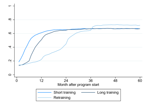
Figure 1: Average Employment Rate for Different Program Types

The key outcomes of my analysis are individual employment and earnings after program start. They are described in Panel C of Table 1. I consider different employment outcomes which inform about how fast a program participant found a job and how stable their employment was in the years following program participation. Concretely, look at job search duration and at total employment up to 60 months after program start, both measured in days. Since I observe the labor market status of program participants with daily precision, I also study the effects of peer quality on employment more dynamically by considering individual employment probabilities in each month after program start. Figure 1 shows the average employment by program type, up to 60 months after program start. Average employment is below 20 percent directly after the program starts and increases to about 65 to 70 percent after around 40 months. The employment rate takes different paths depending on the program type. Retraining programs which have the longest planned duration are characterized by the slowest increase but ultimately reach the highest level of employment. Because jobseekers in these programs are working toward a vocational degree, there is a particularly high incentive to stay in the program until completion. This can be observed by the yearly kinks.

With regard to earnings, I consider daily earnings in the first job and total earnings up to 60 months after program start. Both earnings outcomes are measured in logs. Since the data contains no information about working hours, daily earnings and total earnings can represent earnings from part-time or full-time jobs. Probably partially explained by different lock-in effects of the programs, individuals in retraining programs accumulate less earnings than individuals in short or long training programs. They also have comparatively lower daily earnings in their first job. Finally, in order to shed some light on the mechanisms behind peer effects, I look at further characteristics of the first job. First, I analyze whether the competence level associated with the first job after program participation is equal or higher to the competence level associated with the target occupation. Second, I investigate whether individuals enter the same firm as any of their peers after the program or if they start working at a firm where any of their peers worked at before starting their program.

5 Empirical Strategy

5.1 Measuring Employability

The objective of this study is to quantify the impact of peer quality on individual post-program labor market outcomes. I focus on the average employment prospects of individual $i^{\prime}s$ peers before program start, referred to as (ex-ante) employability in what follows. I first define employability on the individual level and then construct a measure for peer employability as the leave-one-out sample average of individual $i^{\prime}s$ peers employability in group $g$:

$$\bar{X}_{(-i)g}=\frac{1}{n_{g}}\sum^{n_{g}}_{j\neq i}X_{jg}$$ (1)

For further analyzes I also consider fractions of individuals in different quintiles of the employability distribution and the leave-one-out standard deviation in peer employability. Since I do not observe a measure of employability directly in the data, I summarize individual background characteristics which are likely to contain information on a jobseeker’s employability in a single score. I follow an approach similar to Van den Berg et al. (2019) and define employability as the probability of finding a long-term contract within one year of entering unemployment. Long-term contracts are defined as contracts that last for more than 6 months. For the estimation of the model, I rely on a population of comparable jobseekers that do not participate in any program. The reason for doing so is that the employment status without program participation is unobserved for actual participants.

The procedure is the following: First, I draw a random sample of individuals who enter unemployment in the same years as the program participants but do not participate in any program (1.5 million observations). Second, I apply nearest neighbour matching based on the propensity score to adjust for observable differences between the two groups and draw a matched sample of non-participants (the matching procedure is described in detail in Appendix A.1.1). Third, I estimate a logit model based on this sample of non-participants where I regress their employability on a large set of variables including demographic characteristics, information on health, education, skills, past labor market outcomes as well as information on the local labor market situation (measured at the time individuals enter unemployment). The regression output is displayed in Appendix Table LABEL:tab:employability. Fourth, I use the estimated coefficients to predict employability scores for the sample of participants (out-of sample). Finally, I construct the leave-one-out peer measures using the predicted employability.

The distributions of the predicted individual and average employability are shown in Appendix Figures A.2 and A.3 separately by program type. The individual employability ranges from 0.08 to 0.97 while the average employability is naturally more compact, ranging from 0.2 to 0.9. Overall, the distributions are very similar and largely overlapping across program types indicating that participants are quite comparable across program types in terms of their employability. The fact that participants in retraining have lower initial education (see Section 4) does not directly translate into different employment prospects.

The strongest predictors of employability can be identified from the regression output (Appendix Table LABEL:tab:employability) as training, earnings in the past job, occupation, type of employment, recent and long-term labor market attachment as well as old age and disability. Moreover, time of entry into unemployment and region of residence are of importance. Thus, employability depends to a large extent on individual characteristics, which are malleable, as well as on contextual job search factors.

The employability measure entails a number of advantages compared to an analysis which considers several peer characteristics at the same time. First, it achieves a dimension reduction that allows for a more flexible analysis and an easier interpretation of peer effects without having to estimate a high-dimensional model. Second, it is data-driven and does not rely on any prior knowledge of the strongest predictors of employability. The approach requires no further information than what the caseworker can observe in his assessment of the jobseeker. An assessment of the individual employability could thus be rather easily implemented in practice. I conduct a sensitivity analysis which is presented in Appendix A.3.1 where I also consider several readily available peer characteristics separately. The results suggest that individuals benefit from peers with successful labor market histories and that the proposed measure of peer employability is a good proxy for the labor market attachment of peers.

5.2 Identification of Peer Effects

Two main methodological challenges complicate the empirical analysis of peer effects: the reflection and the selection problem (see e.g., Moffitt, 2001). The reflection problem (Manski, 1993) arises because of the simultaneity in peer behavior meaning that an individual affects his peer’s outcomes and the peers affect the individual’s outcome. In the context of labor market training, program participants might for example affect each other through their job search behavior. This complicates the separate identification of exogenous peer effects, i.e., the influence of average peer characteristics, and endogenous peer effects, i.e., the influence of peer behavior. I do not attempt to separate these effects, but estimate a joint effect. This joint effect is captured by the average peer employability which might proxy peer behavior but is determined before program start.

The selection problem arises because of common unobserved shocks at the group level on the one hand and endogenous peer group formation on the other hand. In my setting peer groups might be endogenously formed if individuals select into specific courses based on unobserved preferences or abilities which are correlated among those belonging to the same peer group. In fact, jobseekers do generally not know who they will be grouped with but they might self-select into specific providers or course depending on the characteristics of the course (i.e., timing, content or location).

My identification strategy builds on a strand of literature in the educational context that exploits idiosyncratic variation in the peer group composition controlling for selection into peer groups by including fixed effects at the school or grade level (e.g., Hoxby, 2000; Ammermueller and Pischke, 2009; Bifulco et al., 2011; Lavy et al., 2012; Elsner and Isphording, 2017; Carrell et al., 2018). Similarly, I control for provider choice and exploit the variation in peer employability between comparable courses offered by the same training providers over time. Moreover, I restrict my attention to providers which offer courses exactly once per month and only compare courses that are four months apart. This restriction is based on the idea that jobseekers can select into specific course months only up to three months after they obtain their voucher.

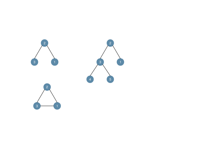
Figure 2: Illustration of the Identification Strategy

Notes: The figure depicts feasible comparison groups ($\lambda_{pc}$) depending on the course start month in rows. These groups are provider-specific and contain courses that are each four months apart. The bottom of the figure illustrates how individuals can select into a specific course month depending on their voucher issuance exemplary for the month April. Columns designate 4-month divisions of the calendar year $\delta_{t}$ which serve as seasonality controls.

The intuition behind the identification strategy is illustrated in Figure 2: A jobseeker obtains a voucher in February and decides to participate in a course starting in April at a particular provider. Her course mates may have obtained their vouchers earlier or later than her, i.e., in the months from January to April. Because of the three month redemption period, the jobseeker cannot be grouped with program participants who obtained their vouchers before January nor with participants who obtain their vouchers starting from May. At the same time, no participant in the April course could select into courses starting before January or later than July. As for the August course, no participant could start a course earlier than May or later than November. In line with this reasoning, I can compare all courses starting in the months of April, August and December at a particular provider without participants being able to self-select into the respective other courses.

Depending on the start dates of the courses, four groups naturally arise which I label month groups: January-May-September, February-June-October, March-July-November and April-August-December. They are listed as rows in Figure 2. Conditional on the choice of provider $p$ and the month group $c$, the entry into a specific course is driven by the voucher issuance date which is unlikely to be manipulated. Participants can sort across provider-specific month groups $\lambda_{pc}$ but not within. I can thus overcome systematic self-selection into groups based on preferences for location and time by comparing only courses at the same provider that are four months apart. Since jobseekers starting courses towards the beginning, middle or end of the year might differ in their characteristics, I further control for aggregate time trends. They are captured by seasonality dummies that correspond to 4-month divisions of the respective calendar year (January to April, May to August and September to October) as shown by the columns $\delta_{t}$ in Figure 2.

Jobseekers have a very limited choice with respect to course content. It needs to match the educational target which is defined during the profiling process with the caseworker and depends on their qualifications but also on the current labor market situation. Nevertheless, it will be important to compare courses of a similar content which I proxy with the competence level and target occupation of a specific course. Note that in my setting conditioning on the provider choice implicitly controls for course content since providers are usually specialized on specific target occupations and thus offer comparable courses over time (see Section 4).

5.3 The Empirical Model

The point of departure of the analysis is the following linear-in-means model which I estimate separately for the three types of training programs:

$$y_{ipct}=\alpha+\gamma X_{ipct}+\theta\bar{X}_{(-i)pct}+\pi W_{pct}+\lambda_{pc}+\delta_{t}+\epsilon_{ipct},$$ (2)

where the outcome of an individual $i$ at a training provider $p$ in month group $c$ and time $t$ (four month interval) is a linear function of the individual’s own observable characteristics $X_{ipct}$, being her own employability and unemployment duration at program start, and the leave-one-out mean employability of individuals in the same course $\bar{X}_{(-i)pct}$. The coefficient of interest is $\theta$, which represents the impact of a marginal increase in the average peer employability on $i$’s outcome. It can be interpreted as a social effect and is a combination of exogenous and endogenous peer effects. Later in the analysis, I introduce more flexibility in how peer effects are modelled and allow for non-linearity.

To implement the identification approach illustrated in Figure 2, I include provider-by-month group, $\lambda_{pc}$ and seasonal fixed effects, $\delta_{t}$ in the model. Provider-month group fixed effects control for all observable and unobservable mean differences across provider-month group combinations that are constant over time. Seasonal fixed effects control for correlated effects which change over time but are the same across providers and month groups. I additionally control for a vector of course-level characteristics, $W_{pct}$ which contains the course size, the average planned duration, weekly hours and total hours spent in practice and class. $W_{pct}$ also includes a set of fixed effects for the target occupation and the competence level of a course. These will take care of differential sorting into courses of specific skills that is constant across providers.

Identification relies on the assumption that the variation in peer employability across courses across courses in a given month group offered by the same provider and after removing seasonality and occupation specific effects is uncorrelated with unobservable determinants of individual post-program outcomes. In other words, I assume that this residual variation results from random fluctuations and is not driven by endogenous sorting into specific courses, i.e., $E[\epsilon_{ipct}\mid X_{ipct},\bar{X}_{(-i)pct},W_{pct},\lambda_{pc},\delta_{t}]=0$. I further assume that there are no spillover effects across courses such that the stable unit treatment value assumption (SUTVA) holds.

5.4 Validity Checks

The empirical strategy will produce unbiased estimates of peer effects if a) the residual variation in peer employability is exogenous and b) peer employability is measured without measurement error.

I investigate the plausibility of an exogenous variation in peer employability with a number of checks. First, I characterize the raw and residual variation in the average peer employability. Figure 3 plots the raw distribution of the variable of interest in the form of a solid line centered at zero. The residual variation after controlling for fixed effects and course controls is depicted in the form of a dashed line. The raw average peer employability ranges has a standard deviation of 0.08. The distributions by program type are summarized in Table 2.They are comparable, with short training courses having a slightly lower raw variation compared to long training and retraining courses. Netting out fixed effects and course controls reduces the variation to about half in all program types with the reduction being strongest for long training. Overall, the remaining variation should be sufficient in order to estimate the effects of interest. Second, I test whether the residual variation in the average peer employability is in line with a variation resulting from random fluctuations. For this I perform a resampling exercise as in Bifulco et al. (2011) and compare the observed residual variation with a simulated variation based on a random group allocation. I find that the variations are closely matching. Third, I check for systematic correlation between own and average peer employability (as in Guryan et al., 2009). I document the absence of such a correlation which provides additional supportive evidence that peer assignment is random. Fourth, I test whether individuals with higher employability sort into certain course months or course types (as measured by the target occupations). Such systematic sorting could cause a selection bias, if not controlled for. I find no evidence for sorting with regard to course timing and some sorting with regard to occupations. This sorting will be taken care of by controlling for provider choice and target occupations as described in Section 5.3. All results, as well as further details on the identifying assumptions as well as the above mentioned tests, are documented in Appendix A.2. Overall, I find strong support for the assumption of the residual variation being idiosyncratic.

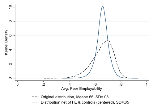
Figure 3: Raw and Net Variation in the Average Peer Employability

Notes: The figure plots the raw distribution of the average peer employability (solid line) and the distribution of the average average peer employability net of provider-month group fixed effects, seasonality fixed effects and course controls. It is centered at the mean of 0.66 (dashed line). SD refers to the standard deviation.

Table 2: Variation in Own and Peer Employability

	Short training				Long training				Retraining
	mean	sd	min	max	mean	sd	min	max	mean	sd	min	max
Panel A - Raw variation
$X_{ipct}$	0.66	0.161	0.08	0.97	0.65	0.163	0.08	0.97	0.66	0.161	0.12	0.97
$\bar{X}_{(-i)pct}$	0.66	0.081	0.20	0.90	0.65	0.081	0.30	0.86	0.66	0.083	0.26	0.88
$\text{SD}(X_{(-i)})_{pct}$	0.15	0.051	0.02	0.36	0.15	0.050	0.02	0.38	0.15	0.051	0.01	0.39
Panel B - Variation net of fixed effects and course characteristics
$X_{ipct}$	0.66	0.161	0.08	0.97	0.65	0.163	0.08	0.97	0.66	0.161	0.12	0.97
$\bar{X}_{(-i)pct}$	0.00	0.049	-0.31	0.25	-0.00	0.046	-0.27	0.28	0.00	0.047	-0.30	0.19
$\text{SD}(X_{(-i)})_{pct}$	0.00	0.036	-0.15	0.21	-0.00	0.035	-0.15	0.18	-0.00	0.037	-0.13	0.20
Observations	28199				9598				8641

Notes: This table shows summary statistics (mean, standard deviation (sd), minimum (min) and maximum (max)) of the employability variables. $X_{ipct}$ designates the own employablity, $\bar{X}_{(-i)pct}$ the leave-one-out mean peer employability, $\text{SD}(X_{(-i)})_{pct}$ the leave-one-out standard deviation of peers’ employability. Panel A displays the figures for the original variables (raw variation). Panel B refers to the residual variation in these variables (net of provider-month group fixed effects, seasonality fixed effects and course controls).

Measurement error in my treatment variable could come from three sources. First, the predicted individual employability could suffer from a prediction error. Such an error could for example occur if not all relevant predictors of employability are included in the model. Due to the richness of the data, this error should be small. Furthermore, it is likely to be orthogonal to the true employability variable and the error term, i.e., classical. Second, an error could come from the fact that employability is measured at entry into unemployment and not directly before program start. For long-term unemployed jobseekers, their employability could deteriorate over time. If jobseekers participate in another labor market program between entering unemployment and the program under consideration, their employability might increase. Both of these changes would not be captured by the proposed employability measure. I run two robustness checks which suggest that a possible error is likely to be small and if anything slightly attenuating the effect. The checks confirm that the proposed measure of peer employability is a good proxy for the labor market attachment of peers. Third, I might not observe all peers in my data which could lead to a mismeasurement of peer variables. I discuss this possibility in detail in Appendix A.2.4. In summary, I argue for the fraction of missing peers to be small and for the missing data to be distributed independently of group assignment and $\epsilon_{ipct}$, conditional on fixed effects and course controls. Under these conditions measurement error would merely cause a small attenuation bias and my results would represent a lower bound of the true peer effects (see Ammermueller and Pischke, 2009, Feld and Zölitz, 2017, Sojourner, 2013).

6 Results

This section presents and discusses the results of the analysis in four parts. First, I examine the effects of an increase in the average predicted peer employability on individual labor market outcomes after program start. Second, I investigate whether there is effect heterogeneity with respect to own employability. Third, I test for non-linearities in the peer effects and estimate a model including the shares of individuals in different quintiles of the employability distribution. Fourth, I assess whether the degree of homogeneity within a group matters by including the group’s standard deviation of employability. All of the analyzes are run separately by program type. Standard errors are clustered at the course level.

6.1 The Effects of Peer Employability on Individual Labor Market Outcomes

6.1.1 Effects on Job Search Duration and Employment

The effects of an increase in the average predicted peer employability on individual employment after program participation are presented in Table 3 separately by program type. Panel A shows the effects on job search duration, Panel B the effects on total employment up to five years after program start. Both outcomes are measured in days. The table presents the effects of a standard deviation increase in the average peer employability ($\bar{X}_{(-i)pct}$) as well as the effect of a standard deviation increase in own employability ($X_{ipct}$).

While an increase in own employability significantly reduces the time individuals look for a job after program start by around three months in all program types, an increase in the average peer employability has no statistically significant effect on job search duration. In contrast, a standard deviation increase in peer employability moderately increases total employment by around 10 to 16 days up until 5 years after program start. The effect is strongest for participants in short programs and smallest for participants in retraining. In comparison, a standard deviation increase in jobseekers’ own employability increases employment by 112 to 126 days.

Table 3: Effects of Peer Employability on Employment

	Short training	Long training	Retraining
	(1)	(2)	(3)
Panel A - Search duration first job (in days)
$\bar{X}_{(-i)pct}$	-7.133	7.970	-1.055
	(5.461)	(8.063)	(7.736)
$X_{ipct}$	-97.471***	-81.633***	-86.889***
	(5.788)	(9.539)	(8.898)
Panel B - Total employment in month 60 (in days)
$\bar{X}_{(-i)pct}$	16.355***	12.884***	10.311**
	(3.303)	(4.835)	(4.812)
$X_{ipct}$	126.024***	120.226***	112.741***
	(3.566)	(5.431)	(5.263)
Provider-Cohort FEs	✓	✓	✓
Seasonal FEs	✓	✓	✓
Additional Controls	✓	✓	✓
Observations	28199	9598	8641

Notes: $X_{ipct}$ designates the own employablity and $\bar{X}_{(-i)pct}$ the leave-one-out mean peer employability. All specifications control for course-level controls and individual unemployment duration at program start. Standard errors (in round brackets) are clustered at the course level. Effects are reported in terms of SD increases (see Table 2). ^∗ $p<0.05$, ^∗∗ $p<0.01$, ^∗∗∗ $p<0.001$

In order to investigate the dynamics behind the effects, I also estimate monthly effects of an increase in the average predicted peer employability on individual employment up to 60 months after program start. Figure 4 shows the results by program type. It depicts the effect estimates (in percentage points) of a one standard deviation increase in the predicted mean peer employability for the months 1-60 after program start. Empty circles indicate that the effect is significant at the 5 percent level. Peer effects materialise for all program types after the average planned program duration, which could be expected given that the program participants reduce their search efforts during the time of the program and that I find no effect on job search duration. At that time, one standard deviation increase in the group’s average employability increases the individual employment probability by around 1 percentage point. The effects are particularly stable for short training, persisting up to 60 months after program start. For long training, the effects are slightly higher in the months 10 to 30, ranging between 1 and 2 percentage points. They fade out around three years after program start. For retraining, I find significant effects only in single months around one, two and four years after program start. It should be kept in mind, that the sample of participants in long training and retraining is much smaller compared to the sample of participants in short training which reduces the power to identify any effect there.

Overall, these findings suggest that exposure to a more employable peer group does not necessarily lead to a faster integration of participants into the labor market but rather increases employment stability. The effect size is moderate and amounts to 9-12 percent of the individual effect, representing a reasonable size. Previous evaluation studies of the same types of programs in Germany, find that program participation increases the employment probability by 10 to 20 percentage points in the long run (see e.g., McCall et al., 2016, Card et al., 2018). In comparison, a peer effect of one percentage point seems like a moderate and realistic increase. However, a direct comparison of the effect sizes is difficult, since the peer effects analyzed here have to be interpreted conditional on participation.

6.1.2 Effects on Earnings

Table 4 presents the effects of a more employable peer group on individual daily earnings in the first job (Panel A) and total earnings in the first five years after program participation (Panel C). Again, the effects correspond to a standard deviation increase in peer and own employability and are displayed separately by program type. Since around 10 percent of program participants are never employed within the relevant observation window, I also estimate the effects on earnings for the sample of participants in employment. Specifically, I consider daily earnings in the first job in the sample of program participants who found a job up to December 2016 (Panel B) and total earnings in the sample of participants that were employed at least once in the first 60 months after program participation (Panel D).

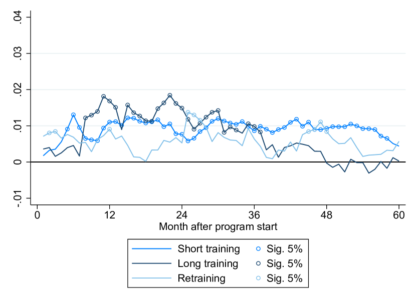
Figure 4: Monthly Effects of Peer Employability on Individual Employment

Notes: The figure depicts the estimated effects (in percentage points) of a one standard deviation increase in the predicted mean peer employability on the individual employment probability in the months 1-60 after program start. Significant effects at the 5 percent level are marked by circles. On top of the mean peer employability, the underlying model includes the individual ex-ante employability, a vector of course-level controls, occupation and provider-by-cohort and seasonal fixed effects. Standard errors are clustered at the course level.

I find that a one standard deviation increase in the average peer employability increases daily earnings in the first job by 3.6 percent for participants in short training. The effect is robust to excluding individuals who did not find a job until the end of the observation window. For participants in long training, the effect of a more employable peer group is zero in the full sample but positive and around 2 percent in the restricted sample. This suggests that participants in long training who are able to find jobs, also experienced an increase in earnings when being exposed to a more employable peer group. For participants in retraining, I find a negative effect on daily earnings of 2.4 to 2.9 percent.

Also in the long run, earnings are affected by an increase in the average employability of peers. I find an effect of 7 percent on total earnings in the first 5 years after program participation for participants in short training which corresponds to about 1100 euro. The effect for participants in long training amounts to 4.5 percent but is not precisely estimated in the full sample. The effects on total earnings are slightly smaller but statistically significant when conditioning on employment. I do not find any effect for individuals in retraining.

Notice that the effect of own employability on earnings in the short and long-run is much larger in the full sample compared to the sample conditioning on employment. This can be explained by own employability picking up the effect of finding a job. Generally own employability does not have a positive effect on earnings in the first job after conditioning on employment. It is only significant for participants in retraining and negative. This suggests that some of the determinants of employability are negatively associated with daily earnings.

In sum, the results point out clear differences between program types. I find large earnings effects in classic vocational training programs suggesting that participants in these programs are able to find better-paid jobs after interacting with more employable peers. Also in the long run, positive earnings effects materialize which cannot be explained by more days in employment. In retraining, an exposure to a better peer group negatively affects participants’ daily earnings in the first job but has no effect on total earnings in the long run. The negative effect on earnings directly after program start is thus not persistent and jobseekers’ earnings recover. Overall, peer effects are not very sensitive to restricting the sample to employed individuals.

Table 4: Effects of Peer Employability on Earnings

	Short training	Long training	Retraining
	(1)	(2)	(3)
Panel A - Log earnings first job
$\bar{X}_{(-i)pct}$	0.031***	-0.008	-0.028**
	(0.008)	(0.015)	(0.014)
$X_{ipct}$	0.087***	0.037**	0.043***
	(0.009)	(0.016)	(0.016)
N	28199	9598	8641
Panel B - Log earnings first job (if $>$ 0)
$\bar{X}_{(-i)pct}$	0.036***	0.021*	-0.024**
	(0.007)	(0.012)	(0.011)
$X_{ipct}$	0.008	-0.016	-0.038***
	(0.007)	(0.013)	(0.013)
N	24391	8228	7527
Panel C - Log total earnings in month 60
$\bar{X}_{(-i)pct}$	0.067***	0.045	-0.005
	(0.017)	(0.029)	(0.026)
$X_{ipct}$	0.460***	0.426***	0.407***
	(0.021)	(0.033)	(0.035)
N	28199	9598	8641
Panel D - Log total earnings in month 60 (if $>$ 0)
$\bar{X}_{(-i)pct}$	0.050***	0.031**	0.010
	(0.008)	(0.013)	(0.013)
$X_{ipct}$	0.191***	0.211***	0.179***
	(0.009)	(0.016)	(0.016)
N	25862	8796	8063
Provider-Cohort FEs	✓	✓	✓
Seasonal FEs	✓	✓	✓
Additional Controls	✓	✓	✓

Notes: $X_{ipct}$ designates the own employablity and $\bar{X}_{(-i)pct}$ the leave-one-out mean peer employability. All specifications control for course-level controls and individual unemployment duration at program start. Standard errors (in round brackets) are clustered at the course level. Effects are reported in terms of SD increases (see Table 2). Earnings are in prices of 2010 and measured in log(euro). ^∗ $p<0.05$, ^∗∗ $p<0.01$, ^∗∗∗ $p<0.001$

6.1.3 Interpretation and Mechanisms

Since participants do not fundamentally differ in their employability across program types, differences in effects are likely to originate from the features of the programs and the mechanisms at work. In the following, I will interpret the results and discuss how the mechanisms presented in Section 3 could apply to the different types of programs.

I find comparable effects for short and long vocational training programs, with the effects for short training being slightly larger. As indicated by the name, these programs differ primarily in their duration but attract comparable types of jobseekers. One difference is that participants in short training have a stronger labor market attachment and complete the program earlier in their unemployment spell. In both programs exposure to a more employable peer group increases individual employment stability and earnings but has no effect on job search duration. Several of the proposed mechanisms are inconsistent with the documented results. First, competition and shifts in self-perception can be ruled out as dominant channels since they would predict negative peer effects on employment stability and earnings. Second, social conformity is unlikely to be a major driver since program participants do not reduce their job search duration when exposed to a more employable peer group. Third, if course instructors were responding endogenously to the peer group composition, I would expect such behavior to occur equally across training programs.

Two remaining plausible channels behind peer effects in classic vocational training programs are thus peer-to-peer learning and peer networks. These programs partly build on already existing occupational competences, which are expanded in the course of the training. Highly employable participants might thus hold a relevant set of skills and networks that spill over to other course participants. As pointed out in Section 3, such spillovers might help program participants to find well-paid first jobs and allow for more successful careers also in the longer run. Formally testing whether peer-to-peer learning or networks are driving the effects is difficult with the administrative data at hand. I provide indirect evidence for these two mechanisms in Table 5. First, I test for skill spillovers, by analysing whether a better peer group affects the competence level program participants acquire during the training (Panel A). For short training, I find that the probability of jobseekers finding a first job with a competence level higher than or equal to the competence level of the program’s target occupation is increasing when they are exposed to more employable peers. The effect is not significant for long training and retraining. This might be explained by the fact that participants in short training have a more relevant set of pre-existing skills to share with their peers compared to participants in longer programs which involve training in newer content. Second, I test for the relevance of peer networks by evaluating whether referrals to the latest employer are more likely in highly employable peer groups. Specifically, I estimate whether the individual probability of taking up a job at the firm where any of the peers worked in their last job depends on the average peer employability. As shown in Panel B of Table 5, I do not find any evidence for effects on referrals to a past employer for any of the program types. This suggests that an exchange of information about previous employers is not the main driver behind the documented peer effects. Nonetheless, jobseekers could still benefit from more general information about job search and the network of peers that goes beyond the latest employer.

Table 5: Mechanisms relating to the first job

	Short training	Long training	Retraining
	(1)	(2)	(3)
Panel A - Prob. of the competence level in first job being
the same or higher than in target occupation
$\bar{X}_{(-i)pct}$	0.008***	-0.001	-0.003
	(0.003)	(0.004)	(0.004)
$X_{ipct}$	-0.001	0.006	-0.006
	(0.003)	(0.005)	(0.005)
N	19308	6996	6794
Panel B - Prob. to work in a firm any peer worked at (in last job)
$\bar{X}_{(-i)pct}$	0.000	0.000	0.000
	(0.001)	(0.001)	(0.001)
$X_{ipct}$	0.000	0.000	0.001
	(0.001)	(0.001)	(0.001)
N	28199	9598	8641
Panel C - Prob. to work in the same firm as any peer (in first job)
$\bar{X}_{(-i)pct}$	0.001	-0.001	0.003***
	(0.001)	(0.001)	(0.001)
$X_{ipct}$	-0.000	-0.000	0.000
	(0.001)	(0.001)	(0.001)
N	28199	9598	8641
Provider-Cohort FEs	✓	✓	✓
Seasonal FEs	✓	✓	✓
Additional Controls	✓	✓	✓

Notes: $X_{ipct}$ designates the own employablity and $\bar{X}_{(-i)pct}$ the leave-one-out mean peer employability. All specifications control for course-level controls, individual employability and unemployment duration at program start. Standard errors (in round brackets) are clustered at the course level. Effects are reported in terms of standard deviation increases (see Table 2). ^∗ $p<0.05$, ^∗∗ $p<0.01$, ^∗∗∗ $p<0.001$

Peer effects in retraining differ from classic vocational training programs particularly with respect to earnings. Being exposed to a more employable peer group in retraining has no effect on job search duration, a more moderate effect on employment stability, a negative effect on earnings in the short run and no effect on earnings in the longer run. As in the case of classic vocational training, also in retraining peer-to-peer learning and the networks of peers might positively affect the skill set of workers and their access to good jobs, but they are expected to do so to a lesser extent. In retraining, every participant is trained in a completely new occupation and the likelihood that existing skills or networks of peers play a role is small compared to classic vocational training programs. Moreover, retraining programs are comparatively long, and the ex-ante employability of participants may no longer matter much at the end of the program. By then, participants in these programs might have a completely new set of skills. This might explain why I find lower peer effects on employment and no long-term earnings effects for these types of programs. Three mechanisms could explain the negative effects on earnings in the first job: social conformity, shifts in self-perception and competition. All of them are expected to affect labor market outcomes rather in the short run and predict negative effects on entry wages. Yet, they differ in their predictions of the impact of more employable peers on job search duration. While shifts in self-confidence and higher competition would be expected to increase job search duration, social conformity would predict the opposite. I find no effect on job search duration but a negative effect on earnings in the first job which suggests that more than one of these mechanisms might apply. There are several reasons, why negative effects on earnings are more likely to occur in retraining compared to classic vocational training programs. First, the programs are longer which gives participants more time to get acquainted and increases the probability that they care about the characteristics and behavior of their peers. Second, participants in retraining are more likely to enter in a direct competition once they exit the program compared to participants in classic vocational training programs. One the one hand, they are more likely to exit the program at the same time after obtaining their vocational degree (see e.g., the jumps in the employment rate in Figure 1). On the other hand, everyone enters the labor market with the same skills for the newly learned profession and might apply for a similar range of jobs. In fact, I show in Panel C of Table 5 that jobseekers in retraining are more likely to start working at the same employer as their peers when they are exposed to a more employable peer group. This further suggests that participants in retraining courses might coordinate in their job search process.

6.2 Robustness Checks

To estimate peer effects, I use a measure of average peer employability that is recorded at the start of unemployment. As explained in Section 5.1, this could cause a bias in the estimated peer effects if the “true” peer employability to which jobseekers are exposed differs from the one I observe. I perform two robustness checks.

First, I test the sensitivity of results to participants attending another program within the same unemployment spell. Specifically, I exclude those individuals who attend any other labor market program between entering unemployment and the program of interest from the sample. This concerns 20 to 30 percent of jobseekers. Possible programs are other training programs, short activation measures and wage subsidies. Appendix Table A.5 presents the results of this exercise for the two main outcomes total employment and total earnings by month 60. The resulting peer effects are qualitatively similar to the main effects reported in Tables 3 and 4 with effect sizes being slightly larger. This suggests that not considering the participation of jobseekers in other programs may lead to a small attenuation bias.

Second, I take into account the average time that peers spend in unemployment. Our main treatment variable measures employability by the probability that jobseekers find a job within one year of becoming unemployed. However, this variable does not account for the duration of unemployment beyond one year in the peer group. I thus estimate an augmented model which includes both peer measures. The results are presented in Appendix Table A.6. They show that increasing the average duration of unemployment in the peer group negatively affects individual employment and earnings after the program. In other words, a reduction in the duration of peer unemployment has a positive effect on individual labor market outcomes. Furthermore, including the average duration of peer unemployment reduces the effect of the mean peer employability by around 50 percent. Jointly, an increase in the average peer employability by one standard deviation and a decrease in the average duration of peer unemployment by one month results in a similar effect size as in the main specification presented in Tables 3 and 4. This suggests that the average peer employability is successfully proxying for the effect of the average unemployment duration in the group. This is not surprising given that individual employability and the unemployment duration at program start are negatively correlated (See Appendix Figure A.11).

In a third robustness check, I aim to rule out that the effects I estimate are endogenously driven by program participants that know each other from their previous job. This could bias the peer effects if these jobseekers select into the same courses based on similar preferences or characteristics. I thus exclude all courses from the sample where more than 20 percent worked at the same firm before entering the program. The results are reported in Appendix Table A.7. They are very similar to the results of the main analysis with the effects on employment being slightly attenuated. In contrast to the main analysis, I now find a significant reduction of the search duration for the first job for participants in short training.

6.3 Does the effect depend on one’s own employability?

Both empirical and theoretical findings in the education literature suggest that students of different ability levels benefit differently from peer ability (e.g., Burke and Sass, 2013, Carrell et al., 2013, Feld and Zölitz, 2017). Further, the program evaluation literature has shown vocational training programs to be more effective for jobseekers with relatively bad employment prospects (Card et al., 2018). Therefore, I test whether individuals heterogeneously respond to the average employability in their group depending on their own employability.

Table 6: Heterogeneity in Effects of Peer Employability Depending on Own Employability

	Short training	Long training	Retraining
	(1)	(2)	(3)
Panel A - Total employment in month 24
PE low employability	6.517***	8.028***	2.198
	(1.610)	(2.499)	(2.692)
PE high employability	2.810	1.792	3.118
	(1.746)	(2.792)	(3.172)
P-value difference	0.045	0.032	0.769
Panel B - Total employment in month 60
PE low employability	16.436***	14.920**	9.851*
	(3.827)	(5.933)	(5.946)
PE high employability	9.366**	-3.034	3.592
	(4.101)	(6.472)	(5.945)
P-value difference	0.107	0.014	0.356
Panel C - Log total earnings in month 60
PE low employability	0.071***	0.072**	0.007
	(0.020)	(0.034)	(0.035)
PE high employability	0.036*	-0.040	-0.052*
	(0.020)	(0.035)	(0.031)
P-value difference	0.121	0.005	0.142
Provider-Cohort FEs	✓	✓	✓
Seasonal FEs	✓	✓	✓
Additional Controls	✓	✓	✓
Observations	28199	9598	8641

Notes: All specifications control for course-level controls, individual employability and unemployment duration at program start. Standard errors (in round brackets) are clustered at the course level. Peer effects (PE) are reported in terms of SD increases (see Table 2). Earnings are in prices of 2010 and measured in log(euro). ^∗ $p<0.05$, ^∗∗ $p<0.01$, ^∗∗∗ $p<0.001$

I estimate the effects of peer employability on post-program employment and earnings based on the main specification, separately by type of participant. To categorize individuals’ own employability, I define program participants with a predicted employability below the sample median as participants with a low employability and participants with an employability greater or equal to the median as participants with a high employability. The results are displayed in Table 6. Participants with a low employability benefit clearly more from being exposed to a better peer group compared to participants with a high employability in short and long vocational training. The effects on total employment up two years after program start (Panel A) and up to five years after program start (Panel B) are both significant for low types but not significant or significantly lower for high types. The same pattern arises for the effect on earnings up to five years after program start (Panel C). For retraining, participants of low employability benefit more in terms of employment and loose out less in terms of earnings. Nevertheless, the differences in effects are estimated too imprecisely in order to draw strong conclusions.

In sum, these results suggest that participants who are less employable ex-ante draw the highest benefits from being surrounded by more employable peers. They might be able to particularly benefit from the knowledge, skills or networks of better peers and thereby increase their own chances on the labor market.

6.4 Looking Beyond the Average

So far the analysis has focused on how the average outcome of a randomly chosen program participant would change in expectation if the average peer employability was marginally increased. This could for example be achieved by admitting a higher share of employable individuals to programs. However, in order to understand how we could optimally assign jobseekers to programs, we need to understand whether peer effects are truly linear-in-means.

6.4.1 A model of fractions

I first estimate a more flexible version of model (2) that includes the fractions of peers in the top and bottom quintiles of the employability distribution instead of the average peer employability. The fraction of peers in the middle quintiles serves as the reference category. Everything else remains the same. Table 7 displays the results for the two long-term employment and earnings outcomes in separate panels. The first and second row of each panel report the effects of a 10 percentage point increase in the fraction of peers in the top and bottom quintile respectively accompanied by a reduction in the fraction of peers in the middle quinitiles. The third row reports the effect of the same increase in the fraction of peers in the top quintile accompanied by a reduction in the fraction of peers in the bottom quintile (difference in coefficients).

I find clear evidence for non-linearities in the effects for participants in short training. Increasing the fraction of peers in the middle or top quintiles (and reducing the fraction of peers in the bottom quintile respectively) results in an effect of a similar size. Cumulative employment increases by 16 and 22 days respectively, the effects not being significantly different from each other. Replacing peers in the middle of the distribution by peers in the top increases the effect on cumulative employment only by 6 days (see Panel A). The effect pattern is similar for cumulative earnings (Panel B). An increase of the fraction of peers in the middle or top quintiles increases earnings by a similar amount.

I cannot reject linearity in peer effects for long training and retraining. Here, the average participant benefits similarly from an increase in the fraction of peers in the top quintile, independently of whether the fraction of peers in the middle or bottom quintiles are reduced in turn. Highly employable peers are thus the driver behind the positive effect. The effects on cumulative earnings are not statistically different from zero for these two types of programs but point to a similar relationship.

Overall, these findings inform about which participants drive the peer effects. While it is mostly highly-employable peers at the top of the distribution in long training and retraining, it is peers from the top and the middle of the employability distribution in short training. There only a slight increase in the average peer employability can be very effective in increasing individual labor market prospects.

Table 7: Non-linearity in Effects - Top versus Bottom Quintile

	Short training	Long training	Retraining
	(1)	(2)	(3)
Panel A - Total employment in month 60
Fraction of peers in top quintile	5.906*	16.541***	13.443***
	(3.139)	(5.008)	(4.936)
Fraction of peers in bottom quintile	-16.524***	-0.310	1.378
	(3.124)	(5.124)	(5.020)
Difference top - bottom quintile	22.431***	16.851***	12.064*
	(3.965)	(5.864)	(6.209)
Panel B - Log total earnings in month 60
Fraction of peers in top quintile	0.006	0.041	-0.022
	(0.016)	(0.028)	(0.024)
Fraction of peers in bottom quintile	-0.078***	-0.010	0.000
	(0.016)	(0.029)	(0.028)
Difference top - bottom quintile	0.084***	0.051	-0.022
	(0.021)	(0.035)	(0.033)
Provider-Cohort FEs	✓	✓	✓
Seasonal FEs	✓	✓	✓
Additional Controls	✓	✓	✓
Observations	28199	9598	8641

Notes: All specifications control for course-level controls, individual employability and unemployment duration at program start. Standard errors (in round brackets) are clustered at the course level. Effects are reported in terms of 10 percentage point increases. Earnings are in prices of 2010 and measured in log(euro). ^∗ $p<0.05$, ^∗∗ $p<0.01$, ^∗∗∗ $p<0.001$

6.4.2 A model accounting for peer group heterogeneity

I apply another popular modelling approach proposed by Booij et al. (2017) that allows for non-linear peer effects and tests whether the heterogeneity in the group plays a role. Individuals might not only be affected by the average quality of the group but benefit from similar coursemates as for example implied by the cognitive learning theory (Bandura, 1986; Schunk, 2012). For this, I augment equation (2) with $\text{SD}(X_{(-i)pct})$, the standard deviation of employability of the other jobseekers in individual $i$’s group. Then, I gradually introduce more flexibility in the model by interacting the peer variables $\bar{X}_{(-i)pct}$ and $\text{SD}(X_{(-i)pct})$ and including interactions with jobseekers own employability ($X_{ipct}$). The fully interacted model allows for both the mean and the dispersion of peer employability to affect outcomes and accounts for effect heterogeneity with respect to own employability. For this approach, all employability variables are centered at mean zero and multiplied with the respective residual standard deviation. This allows us to interpret the effects at the sample average in terms of a standard deviation increase.

The results are presented in Table 8 for total employment in month 60. Columns (1), (4) and (7) add the SD of peer employability to the linear-in-means specification for different program types. Compared to the linear-in-means model in Table 3, the coefficients for mean employability decrease across all program types. The decrease is strongest for participants in short training and minimal for participants in long training. The coefficient of the SD of peer employability is negative across all program types, suggesting that a larger dispersion of peer employability in the group is detrimental to post-program employment. The effect is only significant for short training. Columns (2), (5) and (8) additionally include the interaction term between the two peer variables and thus allow for some complementarity in effects. The coefficients on the interaction term are negative for short training and retraining but only marginally significant. This suggests that increasing peer group heterogeneity is more detrimental in groups with a higher average peer employability. Columns (3), (6) and (9) add interaction terms own employability. In contrast to the findings presented in Table 6, this fully flexible model does not suggest that the effects from increasing the average peer employability significantly vary with own employability. However, there is some heterogeneity in effects from increasing the dispersion in the group. More employable jobseekers seem to suffer more from an increased group heterogeneity.

Table 9 shows the results of the same models for the outcome total earnings in month 60. They are qualitatively comparable. Being exposed to more employable peers increases earnings but a higher peer group heterogeneity has a negative impact. This impact is larger for more employable groups and jobseekers. Nevertheless, effects are less precisely estimated. Peer variables are only jointly significant for participants in short training, which represent the largest sample.

In summary, this analysis confirms the analysis based on fractions of high and low-employability jobseekers (Table 7). Particularly, in short training peer effects do not seem to be linear-in-means but vary with the distribution of peer employability. In these types of programs, peers at the middle of the employability distribution are important in driving peer effects and putting more weight to the extremes of the distribution is detrimental. Positive effects generated by highly-employable peers do not outweigh negative effects generated by a larger fraction of low-employability peers. For long training and retraining the hypothesis of linear-in-means effects cannot be clearly rejected.

Differences in effects between programs may be linked to the mechanisms discussed in Section 6.1.3. If skill spillovers are the dominant driver behind peer effects in short training, these might not only come from peers at the top but also in the middle of the employability distribution. Overall, we should interpret these differences with caution. The lack in power of estimates in the samples of participants in long training and retraining prevents us from making strong statements.

Table 8: Group Heterogeneity - Effects on total employment in month 60

	Short training			Long training			Retraining
	(1)	(2)	(3)	(4)	(5)	(6)	(7)	(8)	(9)
$\bar{X}_{(-i)pct}$	11.995∗∗	12.267∗∗∗	11.843∗∗	12.557∗	12.558∗	10.776∗	7.604	8.005	6.918
	(3.680)	(3.677)	(3.736)	(5.144)	(5.149)	(5.251)	(5.297)	(5.317)	(5.359)
$\text{SD}(X_{(-i)})_{pct}$	-9.842∗∗	-10.322∗∗	-11.511∗∗	-0.804	-0.396	-1.039	-5.713	-6.941	-7.095
	(3.444)	(3.458)	(3.504)	(5.153)	(5.255)	(5.320)	(5.219)	(5.361)	(5.403)
$\bar{X}_{(-i)pct}$*$\text{SD}(X_{(-i)})_{pct}$		-2.828	-1.740		1.154	1.357		-3.010	-2.576
		(1.618)	(1.646)		(2.274)	(2.304)		(2.359)	(2.452)
$X_{ipct}$	125.950∗∗∗	125.751∗∗∗	130.896∗∗∗	120.221∗∗∗	120.311∗∗∗	121.086∗∗∗	112.433∗∗∗	112.324∗∗∗	113.427∗∗∗
	(3.566)	(3.566)	(3.816)	(5.432)	(5.435)	(5.802)	(5.254)	(5.252)	(5.703)
$X_{ipct}$*$\bar{X}_{(-i)pct}$			0.878			-3.122			1.375
			(2.102)			(3.216)			(3.423)
$X_{ipct}$*$\text{SD}(X_{(-i)})_{pct}$			-6.579∗			-7.119			-8.925∗
			(2.732)			(3.799)			(4.198)
$X_{ipct}$*$\bar{X}_{(-i)pct}$*$\text{SD}(X_{(-i)})_{pct}$			2.013			-0.356			-1.385
			(1.366)			(1.986)			(1.901)
Provider-month group FEs	✓	✓	✓	✓	✓	✓	✓	✓	✓
Seasonal FEs	✓	✓	✓	✓	✓	✓	✓	✓	✓
Additional controls	✓	✓	✓	✓	✓	✓	✓	✓	✓
F-test (p-values)	0.000	0.000	0.000	0.029	0.055	0.078	0.061	0.078	0.034
Observations	28199	28199	28199	9598	9598	9598	8641	8641	8641

Notes: Effects are estimated separately in the samples short training, long training and retraining. $X_{ipct}$ designates the own employablity, $\bar{X}_{(-i)pct}$ the leave-one-out mean peer employability, $\text{SD}(X_{(-i)})_{pct}$ the leave-one-out standard deviation of peers’ employability. All specifications control for course-level controls and unemployment duration at program start. Standard errors (in round brackets) are clustered at the course level. Effects are reported in terms of standard deviation increases (see Table 2). P-values correspond to a F-test (Peer variables = 0). ^∗ $p<0.05$, ^∗∗ $p<0.01$, ^∗∗∗ $p<0.001$

Table 9: Group Heterogeneity - Effects on total earnings in month 60

	Short training			Long training			Retraining
	(1)	(2)	(3)	(4)	(5)	(6)	(7)	(8)	(9)
$\bar{X}_{(-i)pct}$	0.056∗∗	0.058∗∗	0.055∗∗	0.048	0.048	0.037	-0.013	-0.012	-0.012
	(0.019)	(0.019)	(0.019)	(0.030)	(0.030)	(0.031)	(0.029)	(0.029)	(0.029)
$\text{SD}(X_{(-i)})_{pct}$	-0.024	-0.027	-0.034	0.009	0.016	0.012	-0.016	-0.021	-0.019
	(0.019)	(0.019)	(0.019)	(0.029)	(0.029)	(0.029)	(0.029)	(0.029)	(0.030)
$\bar{X}_{(-i)pct}$*$\text{SD}(X_{(-i)})_{pct}$		-0.015	-0.012		0.021	0.022		-0.012	-0.015
		(0.009)	(0.009)		(0.014)	(0.014)		(0.013)	(0.012)
$X_{ipct}$	0.460∗∗∗	0.459∗∗∗	0.475∗∗∗	0.426∗∗∗	0.428∗∗∗	0.429∗∗∗	0.406∗∗∗	0.406∗∗∗	0.394∗∗∗
	(0.021)	(0.021)	(0.022)	(0.033)	(0.033)	(0.035)	(0.035)	(0.035)	(0.037)
$X_{ipct}$*$\text{SD}(X_{(-i)})_{pct}$			-0.012			-0.038			-0.013
			(0.013)			(0.020)			(0.023)
$\bar{X}_{(-i)pct}$*$\text{SD}(X_{(-i)})_{pct}$			-0.013			-0.022			0.011
			(0.016)			(0.023)			(0.027)
$X_{ipct}$*$\bar{X}_{(-i)pct}$*$\text{SD}(X_{(-i)})_{pct}$			0.013			0.004			-0.004
			(0.008)			(0.013)			(0.011)
Provider-month group FEs	✓	✓	✓	✓	✓	✓	✓	✓	✓
Seasonal FEs	✓	✓	✓	✓	✓	✓	✓	✓	✓
Additional controls	✓	✓	✓	✓	✓	✓	✓	✓	✓
F-test (p-values)	0.000	0.000	0.000	0.029	0.055	0.078	0.061	0.078	0.034
Observations	28199	28199	28199	9598	9598	9598	8641	8641	8641

Notes: Effects are estimated separately in the samples short training, long training and retraining. $X_{ipct}$ designates the own employablity, $\bar{X}_{(-i)pct}$ the leave-one-out mean peer employability, $\text{SD}(X_{(-i)})_{pct}$ the leave-one-out standard deviation of peers’ employability. All specifications control for course-level controls and unemployment duration at program start. Standard errors (in round brackets) are clustered at the course level. Effects are reported in terms of standard deviation increases (see Table 2). P-values correspond to a F-test (Peer variables = 0). ^∗ $p<0.05$, ^∗∗ $p<0.01$, ^∗∗∗ $p<0.001$

7 Conclusion

This paper investigates how labor market outcomes of participants in public sponsored training depend on the peer group composition as measured by the average employability of the peers. Using a number of predetermined characteristics, I construct a summary measure to proxy for employability. It is defined as the predicted probability to find a stable occupation within one year after entering unemployment. To identify a causal effect, I exploit the quasi-random variation in peer employability across courses offered by the same training providers over time.

My results show that the composition of peers has a significant impact on post program labor market outcomes, and that peer effects vary between classic vocational training and retraining. For participants in classic vocational training, a greater average exposure to a more employable peer group leads to a moderate increase in employment and a substantial increase in earnings of 4 to 7 percent. This suggests that individuals with better peers access higher-paying jobs and experience greater employment stability. For participants in retraining, peer effects on employment are slightly smaller and less robust. Additionally, a more employable peer group negatively affects earnings in the first job but this effect does not persist for long. I find effect heterogeneity with respect to participants’ own employability, with low-employability participants benefiting significantly more from a more employable peer group than highly employable participants. Finally, my findings indicate that there are non-linearities in peer effects. In addition to the average peer employability, the distribution of peer employability also matters. An increase in heterogeneity in the peer group while holding the average employability constant negatively affects individual employment and earnings, particularly in short vocational training.

My findings suggest that peer effects in labor market training and the mechanisms behind it depend on the content, organization and objective of programs. Individuals in classic vocational training have a relatively high labor market attachment and are likely to hold valuable skills which they can share with other participants during a course. I find suggestive evidence for such skill spillovers in short vocational training courses. Additionally, individuals in these courses may have active professional networks that could be helpful for their peers. In contrast, more employable participants in retraining are less likely to have a comparative advantage in skills and networks relative to their less employable peers. In these programs, everyone learns a new occupation and faces a new job search environment. Therefore, participants in retraining are more likely to enter in a direct competition once they exit the program compared to participants in classic vocational training programs.

My results bear important insights for policy makers. They suggest that peer effects could be used to increase the effectiveness of training programs through optimal allocation policies. Since training programs are usually not universal but target a specific subset of jobseekers, I focus on policies that assign a limited number of seats to the optimal group of individuals. Furthermore, I only present recommendations for classic vocational training programs for which I find economically meaningful and robust effects. Optimal allocation policies hinge on a number of factors. First, they depend on the direction of peer effects, i.e., whether they are positive or negative. Second, they depend on whether peer effects are linear-in-means or non-linear. Third, they depend on the welfare function of the social planner who might care about the average outcome of individuals or about those most in need. Recent findings by Baird et al. (2023) suggest, that in settings where peer effects are linear-in-means and positive and where one of the mentioned social welfare functions is maximized, assigning a higher fraction of highly employable jobseekers to programs is likely to increase program effectiveness. Similar effects could be expected for long vocational training programs, for which I cannot reject that peer effects are linear-in-means. Deriving optimal allocation rules for short vocational training programs is less straightforward. It would require a modelling approach that takes into account that peer effects vary with the distribution of peer employability and is beyond the scope of this paper. Generally, policy recommendations regarding regrouping policies should be treated with caution since interventions that manipulate the peer composition have been shown to be confounded by endogenous sorting of individuals (Carrell et al., 2013). Finally, in the case of Germany, an assessment would be necessary to determine whether the net effects of a targeted allocation are greater than those of a voucher system, given that jobseekers are currently not assigned to courses but are free in their course choice.

Appendix A Appendix

A.1 Construction of the Employability Score

A.1.1 Matching Based on the Propensity Score

For our employability model to result in unbiased predictions, we need to assume that the relation between the observed predictors in the sample of non-participants and the employability outcome would be the same in the sample of program participants. This is more likely to hold the more comparable jobseekers in both samples are in terms of their characteristics.

I select the most comparable sample of jobseekers who do not enter any program during their unemployment spell applying nearest neighbour matching based on the propensity score (See e.g., Huber et al., 2013, Abadie and Imbens, 2016). For every program participant, I choose 3 most comparable neighbours. The choice is based on the following reasoning: First, allowing for more than one nearest neighbour but limiting the total number of neighbours to a small number addresses the bias-variance trade-off in matching. It keeps the bias small while increasing the efficiency. Second, a higher number of matched individuals quickly increases the amount of computing time involved. Third, the higher the number of neighbours, the more often it happens that a single observation is used many times as a match (since we draw with replacement). I tested the sensitivity of my results to this matching step using only one nearest neighbour or five and do not find any large differences.

The propensity score is estimated as the conditional probability of being in the sample of program participants based on a set of variables that have been identified as sufficient to eliminate any selection bias in the context of program participation (See Lechner and Wunsch, 2013, Huber et al., 2013, Caliendo et al., 2017). I include demographic characteristics, information on education, training, characteristics of the last job, the recent labor market history, as well as variables characterizing the local labor market situation in the model. It is the same set of variables that is later used for the estimation of the employability score.

Table LABEL:tab:balancedness gives an overview of the variables included in the propensity score estimation. It presents averages for the sample of participants (column 1) and non-participants (column 3) as well as the difference in means (column 5) and the standardized bias (column 7). Even though there remain small differences in means for single variables, the standardized bias lies mostly below 25%, which is the reference value given by Rubin (2001).

Appendix Figure A.1 shows the distribution of the predicted propensity scores for program participants and matched non-participants. The curves largely overlap for both groups which indicates that the matching worked well. Common support for individuals with very high propensity scores is violated. Nevertheless, this concerns only a small percentage of program participants. Overall, I am thus sufficiently able to balance the sample of program participants and non-participants based on their observable characteristics and therefore assume that they are also balanced in unobservable characteristics.

For my main analysis, I perform the matching exercise jointly for all program types. To test whether the employability estimation sensitive to heterogeneity in predictors across program types, I run a version of the matching step separately by program types.

Table A.1: Average Characteristics of Participants and Non-participants

	(1)	(2)	(3)	(4)	(5)
	PP	NP	Diff	pval	SB
Month of entry into unemployment
January	0.13	0.13	0	0.46	0.61
Feburary	0.08	0.08	0	0.02	1.7
March	0.09	0.08	0.01	0.12	2
April	0.08	0.08	0	0.87	0.13
May	0.07	0.07	0	0.28	0.87
June	0.07	0.07	0	0.72	0.28
July	0.08	0.08	0	0.83	0.16
August	0.08	0.08	0	0.49	0.69
September	0.09	0.09	0	0.54	0.95
October	0.09	0.09	0	0.38	1.37
November	0.07	0.07	0	0.55	0.59
December	0.07	0.07	0	0.55	0.41
Year of entry into unemployment
2000	0.01	0.01	0	0.14	1.24
2001	0.01	0.01	0	0.2	0.79
2002	0.01	0.01	0	0.31	0.59
2003	0.01	0.01	0	0.8	0.14
2004	0.02	0.02	0	0.89	0.08
2005	0.03	0.03	0	0.39	0.51
2006	0.06	0.06	0	0.45	0.55
2007	0.15	0.14	0.01	0.01	1.96
2008	0.22	0.22	-0.01	0.31	1.34
2009	0.26	0.27	-0.01	0.11	1.86
2010	0.15	0.14	0.01	0	2.18
2011	0.07	0.07	0	0.09	1.11
Federal state
Schleswig-Holstein	0.04	0.04	0	0.89	0.25
Freie und Hansestadt Hamburg	0.04	0.04	0	0.53	1.39
Niedersachsen	0.09	0.1	0	0.66	0.38
Freie Hansestadt Bremen	0.02	0.02	0	0.74	0.46
Nordrhein-Westfalen	0.23	0.23	0.01	0.12	1.38
Hessen	0.05	0.05	0	0.34	0.86
Rheinland-Pfalz	0.04	0.04	0	0.99	0.01
Baden-Wuerttemberg	0.11	0.11	0	0.71	0.27
Bayern	0.16	0.16	0	0.54	0.47
Saarland	0.02	0.02	0	0.77	0.26
Berlin	0.02	0.02	0	0.5	0.85
Brandenburg	0.03	0.03	0	0.12	0.95
Mecklenburg-Vorpommern	0.04	0.05	0	0.59	1.16
Freistaat Sachsen	0.06	0.06	0	0.19	1
Sachsen-Anhalt	0.02	0.02	0	0.06	1.16
Freistaat Thüringen	0.04	0.04	0	0.2	0.9
Demographic characteristics
Younger than 25 years	0.15	0.17	-0.02	0	4.74
25-29 years	0.17	0.17	0	0.46	0.88
30-34 years	0.15	0.14	0.01	0.05	1.81
35-39 years	0.14	0.13	0	0.41	1.08
40-44 years	0.15	0.14	0.01	0.06	1.54
45-49 years	0.13	0.12	0	0.42	0.67
50-54 years	0.09	0.09	0	0.19	1.29
Older than 54 years	0.03	0.03	0	0.99	0.01
Female	0.44	0.44	0	0.7	0.41
German	0.9	0.9	0	0.53	0.48
Single	0.47	0.48	-0.01	0.14	1.54
Married	0.37	0.36	0.01	0.07	1.65
Marital status missing	0.16	0.16	0	0.96	0.07
Children < 15	0.22	0.22	0	0.44	0.9
Children < 3	0.15	0.15	0	0.72	0.49
Single parent	0.07	0.06	0.01	0.1	2.97
Restrictions or disability	0.11	0.11	0	0.71	0.32
No schooling degree	0.07	0.07	0	0.66	0.64
Schooling degree without Abitur	0.73	0.73	0	0.41	0.86
Schooling degree with Abitur	0.17	0.17	0	0.75	0.27
Schooling missing	0.04	0.04	0	0.08	1.69
Without Vocational Training	0.27	0.27	0	0.73	0.43
Vocational Training	0.61	0.61	0	0.88	0.17
Academic Degree	0.07	0.07	0	0.65	0.42
Missing	0.05	0.04	0	0.02	1.83
Job searched: part time	0.06	0.05	0	0.08	1.36
Job searched: full time	0.74	0.72	0.02	0.01	3.51
Job returner	0.03	0.03	0	0.3	1.13
Characteristics of the last job
No last job	0.01	0.03	-0.01	0	8.5
Unskilled/semiskilled tasks	0.09	0.09	0	0.73	0.32
Skilled tasks	0.66	0.65	0.01	0.04	2.15
Complex tasks	0.04	0.04	0	0.18	1.02
Highly complex tasks	0.07	0.07	0	0.93	0.08
Skills missing	0.14	0.15	-0.01	0.04	2.55
Full-time	0.67	0.69	-0.02	0	4.3
Part-time	0.31	0.28	0.03	0	7.25
Working time missing	0.02	0.03	-0.01	0	8.62
LM history relative to unemployment start
Regular EMP 3 months before	0.61	0.63	-0.02	0	4.51
Marginal EMP 3 months before	0.14	0.11	0.03	0	7.68
Part-time EMP 3 months before	0.1	0.1	0	0.87	0.13
In ALMP 3 months befor	0.09	0.1	-0.02	0.01	5.23
OLF 3 months before	0.02	0.02	0	0.28	0.64
Regular EMP 6 months before	0.6	0.62	-0.03	0	5.14
Marginal EMP 6 months before	0.13	0.11	0.02	0	6.81
Part-time EMP 6 months before	0.1	0.1	0	0.23	1
In ALMP 6 months befor	0.09	0.11	-0.02	0.02	5.39
OLF 6 months before	0.03	0.03	0	0.14	1.03
Regular EMP 9 months before	0.59	0.61	-0.02	0	3.47
Marginal EMP 9 months before	0.13	0.1	0.03	0	7.98
Part-time EMP 9 months before	0.1	0.1	0	0.05	1.65
In ALMP 9 months befor	0.09	0.1	-0.01	0.08	3.47
OLF 9 months before	0.04	0.04	0	0.26	0.73
Regular EMP 12 months before	0.59	0.61	-0.02	0	3.96
Marginal EMP 12 months before	0.12	0.1	0.02	0	6.14
Part-time EMP 12 months before	0.1	0.11	-0.01	0.02	1.93
In ALMP 12 months before	0.09	0.1	-0.01	0.19	2.59
OLF 12 months before	0.04	0.05	0	0.03	1.71
Regular EMP 18 months before	0.56	0.57	-0.01	0.01	2.74
Marginal EMP 18 months before	0.12	0.11	0.01	0	4.3
Part-time EMP 18 months before	0.09	0.1	0	0.08	1.44
In ALMP 18 months before	0.09	0.1	-0.01	0.1	3.42
OLF 18 months before	0.05	0.06	0	0.06	1.41
Regular EMP 24 months before	0.52	0.54	-0.02	0	3.17
Marginal EMP 24 months before	0.12	0.11	0.02	0	4.91
Part-time EMP 24 months before	0.08	0.09	0	0.35	0.74
In ALMP 24 months before	0.09	0.1	-0.01	0.19	2.6
OLF 24 months before	0.06	0.07	-0.01	0.01	2.47
Regular EMP 36 months before	0.47	0.48	-0.01	0.04	2.14
Marginal EMP 36 months before	0.12	0.11	0.01	0.02	3.29
Part-time EMP 36 months before	0.07	0.08	0	0.23	0.95
In ALMP 36 months before	0.09	0.09	0	0.68	0.45
OLF 36 months before	0.07	0.08	0	0.06	1.67
Total EMP 6 months before	132.24	132.12	0.11	0.88	0.17
Total ALO 6 months before	38.91	34.81	4.1	0	6.84
Total ALMP 6 months before	15.46	18.28	-2.82	0	6.29
Total EMP 12 months before	261.51	261.72	-0.21	0.88	0.17
Total ALO 12 months before	77.86	68.49	9.37	0	8.78
Total ALMP 12 months before	31.12	35.98	-4.87	0.01	5.96
Total EMP 24 months before	508.95	509.53	-0.58	0.84	0.26
Total ALO 24 months before	156.71	137.98	18.73	0	10.22
Total ALMP 24 months before	62.58	70.4	-7.81	0.02	5.55
Total EMP 60 months before	1168.88	1166.9	1.98	0.79	0.37
Total ALO 60 months before	417.37	379.1	38.27	0	9.26
Total ALMP 60 months before	158.16	168.84	-10.68	0.03	3.97
Total EMP 120	2107.71	2099.79	7.92	0.49	0.78
Total ALO 120 months before	738.81	669.49	69.32	0	9.6
Total ALMP 120 months before	272.27	281.37	-9.1	0.14	2.26
Number of ALMP 24 months before	0.62	0.64	-0.03	0.21	2.88
Number of ALMP 60 months before	1.26	1.27	-0.01	0.74	0.55
Log. total earnings 12 months before	8.46	8.42	0.05	0.22	1.76
Log. total benefits 12 months before	1.86	1.79	0.07	0.02	2.08
Log. total earnings 24 months before	9.32	9.24	0.08	0.04	3.4
Log. total benefits 24 months before	2.67	2.58	0.08	0.02	2.21
Log. total earnings 48 months before	10.08	9.97	0.11	0.02	4.55
Log. total benefits 48 months before	3.92	3.8	0.12	0	3.04
Log. total earnings 60 months before	10.31	10.19	0.12	0.01	5.16
Log. total benefits 60 months before	4.43	4.35	0.08	0.06	1.94
Log. total earnings 120 months before	10.99	10.84	0.15	0	6.79
Log. total benefits 120 months before	5.91	5.68	0.22	0	5.42
Regional characteristics (at district level)
Local unemployment rate	8.57	8.47	0.09	0	2.64
Population density	776.83	765.49	11.34	0.27	1.29
Employment share primary sector	1.86	1.91	-0.05	0.02	2.58
Employment share secondary sector	26.17	26.31	-0.14	0.12	1.61
Employment share third sector	71.97	71.78	0.19	0.05	1.97
GDP per capita	30.68	30.64	0.04	0.76	0.34
No regional information	0.08	0.09	0	0.34	1.53
Observations	47279	96809

Notes: This table displays the average characteristics of the sample of program participants (PP) and the weighted average characteristics of the sample of matched non-participants (NP) in columns (1) and (2), respectively. Column (3) displays the difference in means and column (4) the standardized bias (SB) calculated for each characteristic $X_{k}$ as $SB_{k}=\frac{|E_{cs}(X_{k})-E_{p}(X_{k})|}{\sqrt{(V_{cs}(X_{k})+V_{p}(X_{k}))/2}}\times 100$.

A.1.2 The Employability Score and Group Size

Table A.2: Predictors of the Probability to be Employed 12 Months after UE Entry

	Coefficient	SE
	(1)	(2)
Demographics
Younger 25 years	-0.055	(0.067)
30-34 years	-0.031	(0.062)
35-39 years	-0.014	(0.060)
40-44 years	-0.040	(0.059)
45-49 years	-0.082	(0.061)
50-54 years	-0.139	(0.073)
Older 54 years	-0.691∗∗∗	(0.091)
Female	0.505	(0.336)
Non-German	0.035	(0.053)
Married	0.078∗	(0.034)
Missing	0.087∗	(0.043)
Children < 15	0.176∗∗∗	(0.052)
Children < 3	-0.099	(0.062)
Restrictions or disability	-0.388∗∗∗	(0.041)
No educational degree	-0.156∗	(0.069)
High school degree (Abitur)	-0.080	(0.056)
Educational degree missing	-0.281∗∗	(0.107)
Without Vocational Training	-0.170∗∗∗	(0.043)
Academic Degree	0.101	(0.091)
Vocational degree missing	-0.135	(0.083)
Job searched: Part-time	-0.046	(0.058)
Job searched: Missing	-0.072	(0.039)
Job returner	0.222	(0.117)
Welfare benefits	-0.028	(0.130)
Month and year of entry into unemployment
Feb	-0.098	(0.070)
Mar	-0.336∗∗∗	(0.085)
Apr	-0.355∗∗∗	(0.073)
May	-0.328∗∗∗	(0.083)
Jun	-0.174∗	(0.082)
Jul	-0.380∗∗∗	(0.070)
Aug	-0.376∗∗∗	(0.086)
Sep	-0.391∗∗∗	(0.085)
Oct	-0.244∗∗	(0.084)
Nov	-0.203∗	(0.082)
Dec	0.057	(0.068)
2000	-0.016	(0.095)
2001	-0.208	(0.110)
2002	-0.349∗∗∗	(0.092)
2003	-0.345∗∗∗	(0.087)
2004	-0.353∗∗∗	(0.101)
2005	-0.141	(0.087)
2006	-0.022	(0.072)
2007	0.141∗	(0.060)
2008	-0.196∗∗∗	(0.053)
2010	0.227∗∗∗	(0.053)
2011	0.148∗∗	(0.055)
Residence - Federal state
Schleswig-Holstein	-0.059	(0.118)
Freie und Hansestadt Hamburg	0.088	(0.087)
Niedersachsen	0.115	(0.066)
Freie Hansestadt Bremen	0.023	(0.264)
Hessen	0.230∗∗	(0.085)
Rheinland-Pfalz	0.106	(0.071)
Baden-Wuerttemberg	0.228∗∗∗	(0.062)
Freistaat Bayern	0.177∗∗	(0.059)
Saarland	0.197	(0.126)
Berlin	0.088	(0.093)
Brandenburg	0.146	(0.097)
Mecklenburg-Vorpommern	0.073	(0.126)
Freistaat Sachsen	0.196∗	(0.096)
Sachsen-Anhalt	0.045	(0.096)
Freistaat Thüringen	0.248∗∗	(0.083)
Missing	-0.276	(0.772)
Characteristics of the last job
No last job	-0.022	(0.404)
Unskilled/semiskilled tasks	-0.026	(0.073)
Complex tasks	-0.034	(0.082)
Highly complex tasks	-0.045	(0.094)
Skill level missing	0.055	(0.060)
Part-time	0.025	(0.067)
Time missing	-0.070	(0.347)
Log earnings in last job	0.082∗∗∗	(0.016)
Agriculture, forestry, farming, and gardening	0.254∗∗	(0.090)
Production of raw materials and goods,	-0.044	(0.046)
Construction, architecture and building services	0.084	(0.048)
Natural sciences, geography and informatics	-0.142	(0.117)
Commercial services, trading, sales, tourism	0.036	(0.062)
Business organisation, accounting, law and admin.	-0.044	(0.082)
Health care, the social sector, teaching and education	0.043	(0.105)
Philology, literature, humanities, social sciences, media, art	-0.503∗∗∗	(0.093)
LM history
Regular EMP 3 months before UE entry	0.063	(0.055)
Marginal EMP 3 months before UE entry	0.307∗∗∗	(0.074)
Part-time EMP 3 months before UE entry	-0.033	(0.076)
In ALMP 3 months before UE entry	-0.042	(0.160)
OLF 3 months before UE entry	-0.172∗∗	(0.063)
Regular EMP 6 months before UE entry	0.056	(0.051)
Marginal EMP 6 months before UE entry	0.081	(0.084)
Part-time EMP 6 months before UE entry	-0.263∗∗	(0.084)
In ALMP 6 months before UE entry	0.046	(0.120)
OLF 6 months before UE entry	-0.215∗∗∗	(0.060)
Regular EMP 9 months before UE entry	-0.070	(0.058)
Marginal EMP 9 months before UE entry	0.142	(0.090)
Part-time EMP 9 months before UE entry	0.134	(0.081)
In ALMP 9 months before UE entry	-0.050	(0.164)
OLF 9 months before UE entry	-0.096	(0.062)
Regular EMP 12 months before UE entry	-0.095∗	(0.043)
Marginal EMP 12 months before UE entry	0.134	(0.074)
Part-time EMP 12 months before UE entry	0.020	(0.074)
In ALMP 12 months before UE entry	0.218	(0.122)
OLF 12 months before UE entry	-0.205∗∗	(0.066)
Regular EMP 18 months before UE entry	0.219∗∗∗	(0.044)
Marginal EMP 18 months before UE entry	0.299∗∗∗	(0.067)
Part-time EMP 18 months before UE entry	-0.079	(0.065)
In ALMP 18 months before UE entry	0.323∗∗	(0.109)
OLF 18 months before UE entry	-0.064	(0.054)
Regular EMP 24 months before UE entry	-0.018	(0.038)
Marginal EMP 24 months before UE entry	0.133∗	(0.056)
Part-time EMP 24 months before UE entry	-0.135∗	(0.063)
In ALMP 24 months before UE entry	-0.146	(0.086)
OLF 24 months before UE entry	0.022	(0.055)
Regular EMP 36 months before UE entry	-0.040	(0.036)
Marginal EMP 36 months before UE entry	0.099∗	(0.049)
Part-time EMP 36 months before UE entry	0.026	(0.054)
In ALMP 36 months before UE entry	-0.018	(0.074)
OLF 36 months before UE entry	-0.093	(0.050)
Total EMPL 6 months before UE entry (days)	0.004∗∗∗	(0.001)
Total UE 6 months before UE entry (days)	0.001	(0.001)
Total ALMP 6 months before UE entry (days)	0.001	(0.002)
Total EMPL 12 months before UE entry (days)	-0.000	(0.001)
Total UE 12 months before UE entry (days)	0.000	(0.001)
Total ALMP 12 months before UE entry (days)	0.000	(0.001)
Total EMPL 24 months before UE entry (days)	-0.000	(0.000)
Total UE 24 months before UE entry (days)	0.000	(0.000)
Total ALMP 24 months before UE entry (days)	-0.001	(0.001)
Total EMPL 60 months before UE entry (days)	0.000∗∗∗	(0.000)
Total UE 60 months before UE entry (days)	0.000	(0.000)
Total ALMP 60 months before UE entry (days)	0.000	(0.000)
Total EMPL 120 months before UE entry (days)	0.000∗∗∗	(0.000)
Total UE 120 months before UE entry (days)	-0.000∗∗∗	(0.000)
Total ALMP 120 months before UE entry (days)	-0.000	(0.000)
No of ALMP 24 months before UE entry	0.030	(0.036)
No of ALMP 60 months before UE entry	-0.017	(0.020)
Log total earnings 12 months before UE entry	0.037∗∗	(0.012)
Log total benefits 12 months before UE entry	-0.010	(0.007)
Log total earnings 24 months before UE entry	-0.028∗	(0.013)
Log total benefits 24 months before UE entry	-0.004	(0.007)
Log total earnings 48 months before UE entry	0.041	(0.023)
Log total benefits 48 months before UE entry	-0.020	(0.011)
Log total earnings 60 months before UE entry	0.032	(0.036)
Log total benefits 60 months before UE entry	0.036∗∗	(0.011)
Log total earnings 120 months before UE entry	-0.066	(0.034)
Log total benefits 120 months before UE entry	0.011	(0.006)
Interactions with gender	Yes
Regional LM characteristics	Yes
Observations	96809

Notes: This table displays the coefficients and corresponding standard errors (SE) of a logit regression of the employability measure on individual characteristics measured at the beginning of the unemployment spell in the sample of non-participants. Coefficients based on interaction terms and for regional labor market (LM) characteristics are omitted in the table.
^∗ $p<0.05$, ^∗∗ $p<0.01$, ^∗∗∗ $p<0.001$

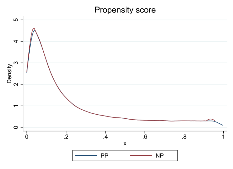
Figure A.1: Predicted P-score (Program Participants and Non-participants)

Notes: This figure displays the distribution of the predicted p-score for program participants (PP) and matched non-participants (NP). P-scores for matches are weighted with the inverse of the matching frequency.

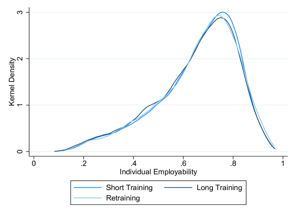
Figure A.2: Distribution of the Individual Predicted Employability by Program Type

Notes: This figure plots the distribution of the predicted individual employbility for the sample of program participants in short training, long training and retraining. It is based on a logit model that is jointly estimated for all prorgam types.

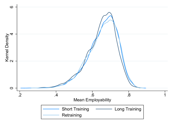
Figure A.3: Distribution of the Average Predicted Employability by Program Type

Notes: This figure plots the distribution of the predicted average employbility for the sample of program participants in short training, long training and retraining. It is based on a logit model that is jointly estimated for all prorgam types.

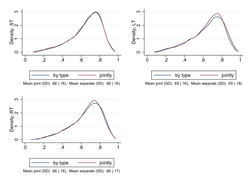
Figure A.4: Distribution of the Predicted Individual Employability (Joint vs. Separate Estimation)

Notes: These figures plot the distribution of the predicted individual employbility for the sample of program participants based on a model that is estimated jointly (red) or separately (blue) by program type. The upper left graph shows the distributions for participants in short training (ST), the upper right graph shows the distributions for participants in long training (LT) and the lower left graph shows the distributions for participants in retraining (RT).

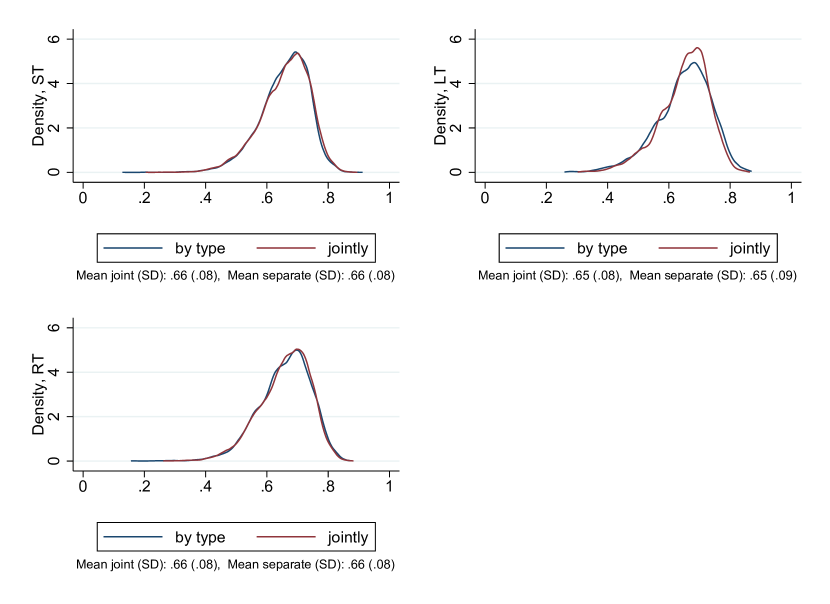
Figure A.5: Distribution of the Predicted Average Employability (Joint vs. Separate Estimation)

Notes: These figures plot the distribution of the predicted average employbility for the sample of program participants based on a model that is estimated jointly (red) or separately (blue) by program type. The upper left graph shows the distributions for participants in short training (ST), the upper right graph shows the distributions for participants in long training (LT) and the lower left graph shows the distributions for participants in retraining (RT).

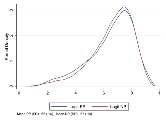
Figure A.6: Individual Predicted Employability (Program Participants and Non-particpants)

Notes: This figure plots the distribution of the predicted individual employbility for the sample of program participants (PP, blue) and the sample of non-participants (NP, red). The distribution is based on a logit model and estimated jointly for all program types. The means and standard deviations (SD) are displayed below the graph.

Figure A.7: Quintiles of the Individual Employability Distribution

Notes: This figure plots the distribution of the predicted individual employbility for the sample of program participants estimated jointly by a logit model. The red lines and corresponding labels mark the thresholds of the second to fifth quintiles.

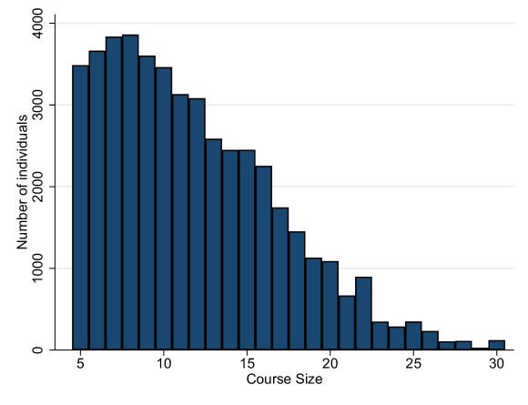
Figure A.8: Distribution of Individuals over Different Course Sizes

Notes: This figure plots the distribution program participants in the estimation sample over different course sizes. It displays the total number of participants on the y-axis.

A.2 Discussion of the Identifying Assumption and Validity Checks

For identification, I need sufficient residual variation in the main peer variables and this variation needs to be exogenous.

For an illustration, consider the error term $\epsilon_{ipct}=\rho_{pct}+\eta_{ipct}$ in equation (2) where $\rho_{pct}$ is a course-specific and $\eta_{ipct}$ a zero-mean random component. For the identifying assumption to hold $\rho_{pct}$ needs to be uncorrelated with all other regressors. That is, there can be no correlated unobservables that vary within month groups and providers. Furthermore, there should be no endogenous sorting into peer groups such that jobseekers strategically manipulate the moment of voucher issuance. I argue that this is highly unlikely given the institutional framework considered. The voucher issuance time highly depends on the availability of caseworkers and the speed of bureaucratic procedures, which are very difficult to predict for jobseekers.

A.2.1 Sorting Over Time and Across Occupations

I thus test for sorting i) over time and ii) across occupations by comparing the distribution of individual employability across different course months and target occupations. Figure A.9 plots the employability distribution across different months of unemployment entry (a) and across months of course start (b). With regard to unemployment entry, there is some sorting of individuals with higher employability into months at the end and at the beginning of the calendar year. Nevertheless, there is no such sorting visible when comparing months of course start. This provides some evidence that the timing of the course start is not directly linked to the timing of unemployment entry. Comparing courses that start in different calender months will thus not exploit variations in course the composition resulting from higher employable jobseekers sorting into specific course months.

I repeat the same exercise in Figure A.9 (c) and compare the distribution of individual employability across different areas of target occupations (so called occupational areas according to the German classification of occupations, KldB 2010). Note that jobseekers are not as evenly distributed across these occupations as compared to course months. While courses with target occupations in health care, the social sector or teaching comprise 23 percent of individuals, courses targeting agriculture comprise only 0.17 percent. Moreover, we do not have information for the target occupation for around 10 percent of individuals. Overall, the employability distributions overlap to a great extent. Nevertheless, there are some notable differences. In particular, jobseekers for whom the target occupation is missing are on average less employable compared to jobseekers in known occupations. In Section 5.2, I argue that controlling for provider choice will mostly take care of a possible selection into courses targeting certain occupations. Additionally controlling for the target occupation will take care of a possible selection bias with regard to occupations that is constant over time and across providers.

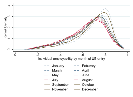
Figure A.9: Sorting in Individual Employability Across Time and Occupation

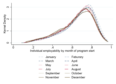
(a) Month of entry into unemployment

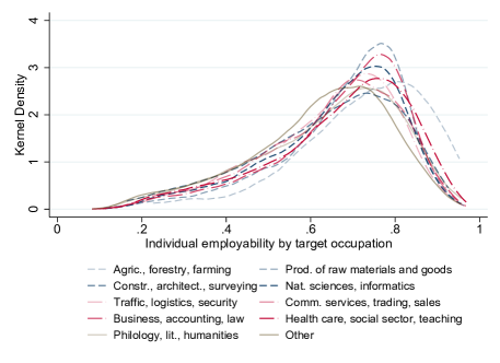
(b) Month of course start

(c) Target occupation

Notes: This figure plots the distribution of the predicted individual employability (kernel density) based on a logit model by month of entry into unemployment (a), month of entry into the program (b) and target occupation (c).

A.2.2 Resampling Test

To provide evidence that the residual variation in my imputed employability variables results from random fluctuation, I ran a series of simulations (similar to Bifulco et al., 2011). In each simulation I randomly reallocate program participants to groups of the same size within the same provider-month group and use this simulated distribution to compute the variation of the predicted peer employability measures. Across 500 simulations and after removing fixed effects and course controls the average residual standard deviation in the simulated peer employability measures ranges from 0.042 to 0.046 (Table A.3). Whereas the simulated residual variation is very close to to observed one for retraining program it is slightly smaller for long training programs. Thus, there might be some excess variation in these types of programs.

Table A.3: Observed and Resampled Standard Deviation

	(1)		(2)		(3)
	ST		LT		RT
Observed SD (raw)	0.081		0.081		0.086
Observed SD (net)	0.049		0.046		0.047
Simulated SD raw	0.075		0.077		0.079
Simulated SD net	0.042		0.044		0.046
Simulations	500		500		500

Notes: This table plots the standard deviation (SD) of the observed peer employability and the average standard deviation of the simulated peer employability measure (over 500 simulations), raw and net of fixed effects and course controls. The figures are displayed seperately by program type: short training (ST), long training (LT), retraining (RT).

A.2.3 Systematic Correlation of Own and Peer Employability

I test whether the residual variation in peer employability is random by regressing the individual employability on the average leave-one-out peer employability and control for the variables on which randomization was conditioned (course level characteristics including occupation and competence level fixed effects, provider-course month effects, time fixed effects). The argument in this classical test for random peer assignment is that if selection into peer groups is ignorable and assignment of peers is quasi-random, then this regression should yield a coefficient of zero. There is a mechanical relationship between the individual and the mean peer employability which stems from the fact that each individual’s peers are drawn from a population with a different mean employability. Following Guryan et al. (2009) I control for that mean, by including the average peer employability at the provider level. Table A.4 shows that there is no significant correlation of the average peer employability and the individual’s own employability.

Table A.4: Exogeneity Test Controlling for the Average Employability at Provider Level

	(1)	(2)	(3)
	Short Training	Long Training	Retraining
Mean peer employability	0.001	-0.002	0.001
	(0.001)	(0.001)	(0.001)
Mean peer employability (provider)	-1.128***	-0.903***	-0.863***
	(0.023)	(0.023)	(0.019)
Provider-Cohort FEs	✓	✓	✓
Seasonal FEs	✓	✓	✓
Additional Controls	✓	✓	✓
Observations	28199	9598	8641

Notes: This table displays the coefficients of a regression of the individual employability on the average employability in the course and at the provider. Standard errors are clustered at the course level. ^∗ $p<0.05$, ^∗∗ $p<0.01$, ^∗∗∗ $p<0.001$

A.2.4 Measurement Error through Unobserved Peers

There is a possibility that I do not observe all individuals in a training program. The data covers all jobseekers who are participating in publicly sponsored training measures and register at the local employment agencies. I do not observe individuals participating in a training program on their own or on their employer’s initiative and do so without registering the employment agencies. There are different groups that could self-select into vocational training programs without being registered. First, there could be individuals who are integrated in the labor market and are either employed or self-employed. At the same time, the likelihood that those individuals would participate in long, full-time courses is very low. If employed, employers would need to grant them leave of absence or in case of self-employment, they would incur major costs of leaving their business. Moreover courses directed at the integration of unemployed individuals into the labor market will not be of great interest for those who already have a job. As for the non-employed individuals, I might not observe women returning to the labor market, non-employed individuals who are not eligible for unemployment assistance and non-registered recipients of social assistance. Nevertheless, all three groups face substantial incentives to register as unemployed if willing to participate in training measures. By registering they could still get access to funding for the course-related costs, for example. By restricting the analysis to full-time courses and excluding courses that are specifically directed at employed individuals the existence of unobserved participants is highly unlikely. A small fraction of unobserved peers would lead to a attenuation bias that is negligible, assuming that there is no selection into courses that specifically relates to quality. Missing and observed data can come from arbitrarily different distributions (e.g., participants missing in the data may be more skilled than the ones observed) but the distribution needs to be independent of group assignment and $\epsilon_{ipct}$ after controlling for fixed effects and course controls (Ammermueller and Pischke, 2009; Sojourner, 2013).

A.3 Further Results

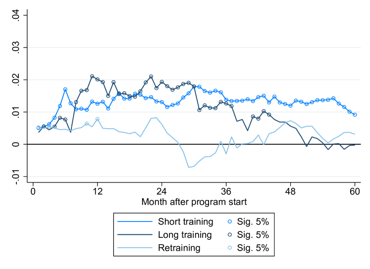
Figure A.10: Monthly Effects of Peer Employability on Regular Employment

Notes: The figure depicts the estimated effects (in percentage points/100) of a one standard deviation increase in the predicted mean peer employability on the individual probability to be employed in a regular job in the months 1-60 after program start. Significant effects at the 5 percent level are marked by circles. On top of the mean peer employability, the underlying model includes the individual ex-ante employability, a vector of course-level controls, occupation and provider-by-month group and seasonal fixed effects. Standard errors are clustered at the course level.

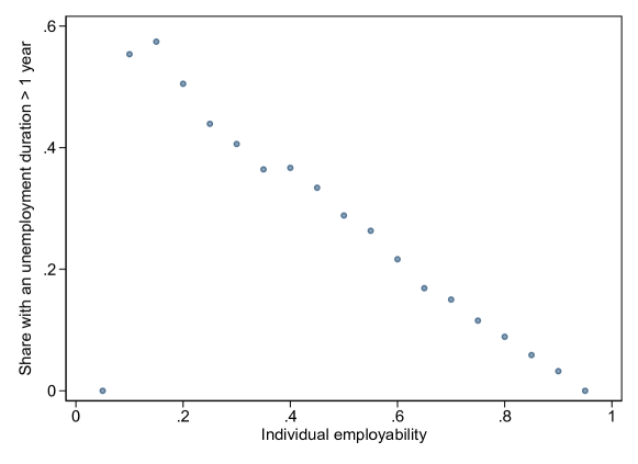
Figure A.11: Own employability and unemployment duration at program start

Notes: This figure plots the average share of jobseekers with an unemployment duration at program start that is larger than one year over bins of 5 percentage points for individual employability. With the exception of the first bin (which is based on few observations) there exists a clear negative relationship between the two variables.

Table A.5: Effects of Peer Employability (Excluding Jobseekers who have Participated in Another ALMP since Becoming Unemployed)

	Short training	Long training	Retraining
	(1)	(2)	(3)
Panel A - Total employment in month 60
$\bar{X}_{(-i)pct}$	20.072***	14.923**	14.269**
	(3.876)	(5.815)	(5.648)
$X_{ipct}$	133.463***	133.630***	126.337***
	(4.162)	(6.652)	(6.672)
Panel B - Log total earnings 60 months after prg. start
$\bar{X}_{(-i)pct}$	0.098***	0.038	0.038
	(0.018)	(0.032)	(0.027)
$X_{ipct}$	0.462***	0.461***	0.417***
	(0.022)	(0.039)	(0.041)
Provider-Cohort FEs	✓	✓	✓
Seasonal FEs	✓	✓	✓
Additional Controls	✓	✓	✓
Observations	21801	7061	6054

Notes: $X_{ipct}$ designates the own employablity and $\bar{X}_{(-i)pct}$ the leave-one-out mean peer employability. All specifications control for course-level controls, individual employability and unemployment duration at program start. Standard errors (in round brackets) are clustered at the course level. Effects are reported in terms of standard deviation increases (see Table 2). ^∗ $p<0.05$, ^∗∗ $p<0.01$, ^∗∗∗ $p<0.001$

Table A.6: Effects of Peer Employability and Unemployment

	Short training	Long training	Retraining
	(1)	(2)	(3)
Panel A - Total employment in month 60
$\bar{X}_{(-i)pct}$	7.209**	8.766*	7.057
	(3.407)	(4.917)	(4.844)
$\bar{UED}_{(-i)pct}$	-5.733***	-3.233***	-2.357**
	(0.708)	(1.054)	(1.050)
$X_{ipct}$	124.353***	119.552***	112.385***
	(3.555)	(5.417)	(5.259)
Panel B - Log total earnings 60 months after prg. start
$\bar{X}_{(-i)pct}$	0.027	0.027	-0.020
	(0.018)	(0.030)	(0.027)
$\bar{UED}_{(-i)pct}$	-0.025***	-0.014**	-0.011*
	(0.004)	(0.006)	(0.006)
$X_{ipct}$	0.453***	0.423***	0.406***
	(0.020)	(0.033)	(0.035)
Provider-Cohort FEs	✓	✓	✓
Seasonal FEs	✓	✓	✓
Additional Controls	✓	✓	✓
Observations	28199	9598	8641

Notes: $X_{ipct}$ designates the own employablity, $\bar{X}_{(-i)pct}$ the leave-one-out mean peer employability, $\bar{UED}_{(-i)pct}$ the leave-one-out unemployment duration of peers. All specifications control for course-level controls and individual unemployment duration at program start. Standard errors (in round brackets) are clustered at the course level. Effects are reported in terms of standard deviation increases (see Table 2). ^∗ $p<0.05$, ^∗∗ $p<0.01$, ^∗∗∗ $p<0.001$

Table A.7: Effects of Peer Employability (Excluding Courses where Participants Worked at the Same Firm)

	Short training	Long training	Retraining
	(1)	(2)	(3)
Panel A - Search duration first job (in days)
$\bar{X}_{(-i)pct}$	-11.887**	-1.462	-3.745
	(5.337)	(7.544)	(7.747)
$X_{ipct}$	-99.164***	-85.589***	-90.683***
	(5.916)	(9.675)	(9.111)
Panel B - Total employment in month 60
$\bar{X}_{(-i)pct}$	14.973***	12.402**	7.266
	(3.347)	(4.884)	(4.674)
$X_{ipct}$	125.608***	120.340***	110.477***
	(3.659)	(5.532)	(5.381)
Panel C - Log earnings first job
$\bar{X}_{(-i)pct}$	0.036***	0.010	-0.029**
	(0.008)	(0.014)	(0.014)
$X_{ipct}$	0.088***	0.047***	0.043**
	(0.009)	(0.016)	(0.017)
Panel D - Log total earnings 60 months after prg. start
$\bar{X}_{(-i)pct}$	0.067***	0.052*	-0.006
	(0.018)	(0.029)	(0.028)
$X_{ipct}$	0.461***	0.430***	0.404***
	(0.021)	(0.034)	(0.036)
Provider-Cohort FEs	✓	✓	✓
Seasonal FEs	✓	✓	✓
Additional Controls	✓	✓	✓
Observations	26810	9215	8178

Notes: $X_{ipct}$ designates the own employablity and $\bar{X}_{(-i)pct}$ the leave-one-out mean peer employability. All specifications control for course-level controls and individual unemployment duration at program start. Standard errors (in round brackets) are clustered at the course level. Effects are reported in terms of standard deviation increases (see Table 2). ^∗ $p<0.05$, ^∗∗ $p<0.01$, ^∗∗∗ $p<0.001$

Table A.8: Heterogeneity in Effects of Peer Employability Depending on Gender

	Short training	Long training	Retraining
	(1)	(2)	(3)
Panel A - Total employment in month 24
PE males	5.603***	7.528***	4.090
	(1.631)	(2.470)	(2.783)
PE females	6.461***	7.614***	3.392
	(1.728)	(2.821)	(3.075)
P-value difference	0.654	0.978	0.825
Panel B - Total employment in month 60
PE males	15.510***	11.737**	12.727**
	(3.896)	(5.678)	(5.678)
PE females	16.526***	13.050**	7.350
	(4.135)	(6.547)	(5.921)
P-value difference	0.826	0.861	0.418
Panel C - Log total earnings in month 60
PE males	0.061***	0.013	0.016
	(0.021)	(0.034)	(0.034)
PE females	0.075***	0.097**	-0.029
	(0.022)	(0.042)	(0.032)
P-value difference	0.592	0.082	0.273
Provider-Cohort FEs	✓	✓	✓
Seasonal FEs	✓	✓	✓
Additional Controls	✓	✓	✓
Observation	28199	9598	8641

Notes: All specifications control for course-level controls, individual employability and unemployment duration at program start. Standard errors (in round brackets) are clustered at the course level. Effects are reported in terms of standard deviation increases (see Table 2). ^∗ $p<0.05$, ^∗∗ $p<0.01$, ^∗∗∗ $p<0.001$

Table A.9: Non-Linearity in Effects - Upper versus Lower Third

	Short training	Long training	Retraining
	(1)	(2)	(3)
Panel A - Total employment in month 60
Fraction highly-employable peers	6.051*	6.262	10.622**
	(3.173)	(4.585)	(4.562)
Fraction low employable peers	-9.807***	-6.308	-3.246
	(2.946)	(5.082)	(4.491)
Difference high-low	15.857***	12.570***	13.867***
	(3.005)	(4.846)	(4.757)
Panel B - Log total earnings in month 60
Fraction highly-employable peers	0.020	0.015	0.015
	(0.017)	(0.026)	(0.024)
Fraction low employable peers	-0.044***	-0.029	0.003
	(0.016)	(0.026)	(0.025)
Difference high-low	0.064***	0.043	0.011
	(0.016)	(0.029)	(0.024)
Provider-Cohort FEs	✓	✓	✓
Seasonal FEs	✓	✓	✓
Additional Controls	✓	✓	✓
Observations	28199	9598	8641

Notes: All specifications control for course-level controls, individual employability and unemployment duration at program start. Standard errors (in round brackets) are clustered at the course level. Effects are reported in terms of 10 percentage point increases. ^∗ $p<0.05$, ^∗∗ $p<0.01$, ^∗∗∗ $p<0.001$

A.3.1 Potential Drivers of Peer Effects in Employability

I investigate potential drivers of the effects in peer employability by including readily available peer characteristics in model (2) which do not rely on a first-step prediction. I test three different models. The first includes the average number of months peers have been employed in the past two years before program start. The second the average number of months peers have been employed in the past 10 years before program start. The third includes the average peer earnings in the two years before program start. All models control for a set of individual level characteristics such as well as the set of fixed effects and course controls used in the main model. The effects of the three peer variables on cumulative employment and earnings are displayed in A.10 as separate rows for the three program types short training (ST), long training (LT) and retraining (RT).

I find that the recent labor market attachment of the peer group is positively associated with individual post-program employment in all three program types. The effect sizes are moderate. Increasing the average number of months in peer employment in the two years before program start by one, increases employment up to five years after program start by up to 9 days. The effect is strongest for individuals in short training and retraining. A one month increase in the average months in peer employment 10 years prior to program start also results in a positive effect on individual employment by one to two days. For the interpretation of the effect sizes, it is important to keep in mind that a one month increase in employment over 10 years represents a smaller increase compared to a one month increase over two years. An increase in the average peer earnings (in the past two years) by 1000 euro results in a longer employment duration of two to three days. We also find some positive effects on cumulative earnings, in particular for individuals in short training.

Overall, the results suggest that individuals seem to benefit from peers with successful labor market histories. This is in line with our findings from the main analysis and suggests that our measure of peer employability is a proxy for the labor market attachment of peers.

Table A.10: The Effects of Other Average Peer Characteristics

	Total employment in month 60				Log total earnings month 60
	(ST)		(LT)	(RT)	(ST)	(LT)	(RT)
Peer earnings in last 2 years (1000 euro)	2.12∗∗∗		1.70∗	3.74∗∗∗	0.01∗∗∗	0.00	0.01∗∗
	(0.46)		(0.77)	(1.03)	(0.00)	(0.00)	(0.00)
Peer months of employment in last 2 years	9.22∗∗∗		5.20∗∗	8.14∗∗∗	0.04∗∗∗	0.01	0.01
	(1.12)		(1.90)	(2.14)	(0.01)	(0.01)	(0.01)
Peer months of employment in last 10 years	0.85∗∗		1.44∗∗∗	1.39∗∗	0.00∗	0.00	0.00
	(0.28)		(0.43)	(0.47)	(0.00)	(0.00)	(0.00)
Individual-level controls	Yes		Yes	Yes	Yes	Yes	Yes
Provider-Cohort FEs	Yes		Yes	Yes	Yes	Yes	Yes
Seasonal FEs	Yes		Yes	Yes	Yes	Yes	Yes
Additional Controls	Yes		Yes	Yes	Yes	Yes	Yes
Observations	28199		9598	8641	28199	9598	8641

Notes: All specifications control for course-level controls, individual age, gender, nationality, education, vocational degree, unemployment duration at program start as well as the individual labor market attachment. Standard errors are clustered at the course level. ^∗ $p<0.05$, ^∗∗ $p<0.01$, ^∗∗∗ $p<0.001$

References

- (1)
- Abadie and Imbens (2016) Abadie, Alberto and Guido W. Imbens (2016). “Matching on the Estimated Propensity Score”, Econometrica, 84(2): 781–807.
- Akerlof and Kranton (2000) Akerlof, G.A. and R.E. Kranton (2000). “Economics and Identity”, The Quarterly Journal of Economics, 115(3): 715–753.
- Ammermueller and Pischke (2009) Ammermueller, Andreas and Jörn-Steffen Pischke (2009). “Peer Effects in European Primary Schools: Evidence from the Progress in International Reading Literacy Study”, Journal of Labor Economics, 27(3): 315–348.
- Antecol et al. (2016) Antecol, Heather, Ozkan Eren, and Serkan Ozbeklik (2016). “Peer effects in disadvantaged primary schools: Evidence from a randomized experiment”, Journal of Human Resources, 51(1): 95–132.
- Arcidiacono et al. (2012) Arcidiacono, Peter, Gigi Foster, Natalie Goodpaster, and Josh Kinsler (2012). “Estimating spillovers using panel data, with an application to the classroom”, Quantitative Economics, 3(3): 421–470.
- Baird et al. (2023) Baird, Matthew D., John Engberg, and Isaac M. Opper (2023). “Optimal Allocation of Seats in the Presence of Peer Effects: Evidence from a Job Training Program”, Journal of Labor Economics, 41(2): 291–509.
- Bandura (1986) Bandura, Albert (1986). Social foundations of thought and action : a social cognitive theory, Englewood Cliffs, NJ:Prentice Hall.
- Behncke et al. (2009) Behncke, Stefanie, Markus Frölich, and Michael Lechner (2009). “Targeting labour market programmes — results from a randomized experiment”, Swiss Journal of Economics and Statistics, 145(3): 221–268.
- Bernheim (1994) Bernheim, B. Douglas (1994). “A Theory of Conformity”, Journal of Political Economy, 102(5): 841–877.
- Bertoni and Nisticò (2023) Bertoni, Marco and Roberto Nisticò (2023). “Ordinal rank and the structure of ability peer effects”, Journal of Public Economics, 217 104797.
- Biewen et al. (2014) Biewen, M., B. Fitzenberger, A. Osikominu, and M. Paul (2014). “The Effectiveness of Public-Sponsored Training Revisited: The Importance of Data and Methodological Choices”, Journal of Labor Economics, 32(4): 837–896.
- Bifulco et al. (2011) Bifulco, Robert, Jason M. Fletcher, and Stephen L. Ross (2011). “The Effect of Classmate Characteristics on Post-Secondary Outcomes: Evidence from the Add Health”, American Economic Journal: Economic Policy, 3(1): 25–53.
- Black et al. (2013) Black, Sandra E., Paul J. Devereux, and Kjell G. Salvanes (2013). “Under Pressure? The Effect of Peers on Outcomes of Young Adults”, Journal of Labor Economics, 31(1): 119–153.
- Booij et al. (2017) Booij, Adam S., Edwin Leuven, and Hessel Oosterbeek (2017). “Ability Peer Effects in University: Evidence from a Randomized Experiment”, The Review of Economic Studies, 84(2): 547–578.
- Boucher et al. (2014) Boucher, Vincent, Yann Bramoulle, Habiba Djebbari, and Bernard Fortin (2014). “Do peers affect student achievement? Evidence from Canada using group size variation”, Journal of Applied Econometrics, 29(1): 91–109.
- Bramoullé et al. (2009) Bramoullé, Yann, Habiba Djebbari, and Bernard Fortin (2009). “Identification of Peer Effects through Social Networks”, Journal of Econometrics, 150: 41–55.
- Bramoullé et al. (2014) Bramoullé, Yann, Rachel Kranton, and Martin D’Amours (2014). “Strategic interaction and networks”, American Economic Review, 104(3): 898–930.
- Brodaty and Gurgand (2016) Brodaty, Thibault and Marc Gurgand (2016). “Good peers or good teachers? Evidence from a French University”, Economics of Education Review, 54: 62–78.
- Brown et al. (2016) Brown, Meta, Elizabeth Setren, and Giorgio Topa (2016). “Do informal referrals lead to better matches? Evidence from a firm’s employee referral system”, Journal of Labor Economics, 34(1): 161–209.
- Burke and Sass (2013) Burke, Mary A. and Tim R. Sass (2013). “Classroom Peer Effects and Student Achievement”, Journal of Labor Economics, 31(1): 51–82.
- Caliendo et al. (2017) Caliendo, Marco, Robert Mahlstedt, and Oscar A. Mitnik (2017). “Unobservable, but unimportant? The relevance of usually unobserved variables for the evaluation of labor market policies”, Labour Economics, 46: 14–25.
- Calvo-Armengol et al. (2009) Calvo-Armengol, Antoni, Eleonora Patacchini, and Yves Zenou (2009). “Peer Effects and Social Networks in Education”, Review of Economic Studies, 76: 1239–1267.
- Card et al. (2010) Card, David, Jochen Kluve, and Andrea Weber (2010). “Active labour market policy evaluations: A meta-analysis”, The Economic Journal, 120: F452–F477.
- Card et al. (2018) (2018). “What works? A meta analysis of recent active labor market program evaluations”, Journal of the European Economic Association, 16(3): 894–931.
- Carrell et al. (2018) Carrell, Scott E, Mark Hoekstra, and Elira Kuka (2018). “The Long-Run Effects of Disruptive Peers”, American Economic Review, 108(11): 3377–3415.
- Carrell et al. (2013) Carrell, Scott, Bruce I. Sacerdote, and James E. West (2013). “From Natural Variation to optimal Policy? The Importance of Endogeneous Peer Group Formation”, Econometrica, 81(3): 855–882.
- Cingano and Rosolia (2012) Cingano, Federico and Alfonso Rosolia (2012). “People I Know: Job Search and Social Networks”, Journal of Labor Economics, 30(2): 291–332.
- Clark (2003) Clark, Andrew E. (2003). “Unemployment as a Social Norm: Psychological Evidence from Panel Data”, Journal of Labor Economics, 21(2): 323–351.
- Cockx et al. (2023) Cockx, Bart, Michael Lechner, and Joost Bollens (2023). “Priority to unemployed immigrants? A causal machine learning evaluation of training in Belgium”, Labour Economics, 80(102306).
- Colpitts and Smith (2002) Colpitts, Terry and Jeffrey A. Smith (2002). “Targeting Reemployment Services in Canada: The Service and Outcome Measurement System (SOMS) Experience”, in Randall W. Eberts, Christopher J. O’Leary, and Stephen A. Wandner eds. Targeting Employment Services, Kalamazoo, MI: W.E. Upjohn Institute for Employment Research, Chap. 10: 283–308.
- Cooley Fruehwirth (2013) Cooley Fruehwirth, Jane (2013). “Identifying peer achievement spillovers: Implications for desegregation and the achievement gap”, Quantitative Economics, 4: 5–124.
- Cristian Pop-Eleches et al. (2013) Cristian Pop-Eleches, By, Miguel Urquiola, Josh Angrist, Ken Chay, Damon Clark, Rajeev Dehejia, Caroline Hoxby, Chang-Tai Hsieh, Lawrence Katz, Bentley MacLeod, Ofer Malamud, Richard Murnane, Jonah Rockoff, Amy Schwartz, and Douglas Staiger (2013). “Going to a Better School: Effects and Behavioral Responses”, American Economic Review, 103(4): 1289–1324.
- De Giorgi et al. (2010) De Giorgi, G., M. Pellizzari, and S. Redaelli (2010). “Identification of social interactions through partially overlapping peer groups”, American Economic Journal: Applied Economics, 2: 241–275.
- De Giorgi et al. (2012) De Giorgi, Giacomo, Michele Pellizzari, and Gui Woolston Woolston (2012). “Class Size and Class Heterogeneity”, Journal of the European Economic Association, 10(4): 795–830.
- De Grip and Sauermann (2012) De Grip, Andries and Jan Sauermann (2012). “The Effects of Training on Own and Co-worker Productivity: Evidence from a Field Experiment”, The Economic Journal, 122(560): 376–399.
- Doerr et al. (2017) Doerr, Annabelle, Bernd Fitzenberger, Thomas Kruppe, Marie Paul, and Anthony Strittmatter (2017). “Employment and earnings effects of awarding training vouchers in Germany”, Industrial and Labor Relations Review, 70(3): 767–812.
- Duflo et al. (2011) Duflo, Esther, Pascaline Dupas, and Michael Kremer (2011). “Peer Effects, Teacher Incentives, and the Impact of Tracking: Evidence from a Randomized Evaluation in Kenya”, American Economic Review, 101(5): 1739–1774.
- Dustmann et al. (2016) Dustmann, Christian, Albrecht Glitz, Uta Schönberg, and Herbert Brücker (2016). “Referral-based job search networks”, Review of Economic Studies, 83(2): 514–546.
- Eberts et al. (2002) Eberts, Randall W., Christopher O’Leary, and Stephen Wandner (2002). Targeting Employment Services, W.E. Upjohn Institute.
- Elsner and Isphording (2017) Elsner, Benjamin and Ingo E. Isphording (2017). “A Big Fish in a Small Pond: Ability Rank and Human Capital Investment”, Journal of Labor Economics, 35(3): 787–828.
- Epple and Romano (2011) Epple, Dennis and Richard E. Romano (2011). “Peer effects in education: A survey of the theory and evidence”, Handbook of Social Economics, 1(1 B): 1053–1163.
- Falk and Ichino (2006) Falk, Armin and Andrea Ichino (2006). “Clean Evidence on Peer Effects”, Journal of Labor Economics, 24(1): 39–57.
- Feld and Zölitz (2017) Feld, Jan and Ulf Zölitz (2017). “Understanding Peer Effects: On the Nature, Estimation, and Channels of Peer Effects”, Journal of Labor Economics, 35(2): 387–428.
- Frakes and Wasserman (2021) Frakes, Michael D. and Melissa F. Wasserman (2021). “Knowledge spillovers, peer effects, and telecommuting: Evidence from the U.S. Patent Office”, Journal of Public Economics, 198 104425.
- Frölich (2008) Frölich, Markus (2008). “Statistical Treatment Choice”, Journal of the American Statistical Association, 103: 547–558.
- Fu et al. (2019) Fu, Jingcheng, Martin Sefton, and Richard Upward (2019). “Social comparisons in job search”, Journal of Economic Behavior and Organization, 168: 338–361.
- Gaviria and Raphael (2001) Gaviria, Alejandro and Steven Raphael (2001). “School-Based Peer Effects and Juvenile Behavior”, Review of Economics and Statistics, 83(2): 257–268.
- Graham (2011) Graham, Bryan S. (2011). “Econometric methods for the analysis of assignment problems in the presence of complementarity and social spillovers”, in Handbook of Social Economics, volume 1b edition, Chap. 19: 965–1051.
- Guryan et al. (2009) Guryan, Jonathan, Kory Kroft, and Matthew J. Notowidigdo (2009). “Peer Effects in the Workplace: Evidence from Random Groupings in Professional Golf Tournaments”, American Economic Journal: Applied Economics, 1(4): 34–68.
- Heckman et al. (1997) Heckman, James J., Jeffrey Smith, and Nancy Clements (1997). “Making The Most Out Of Programme Evaluations and Social Experiments: Accounting For Heterogeneity in Programme Impacts”, The Review of Economic Studies, 64(4): 487–535.
- Hetschko et al. (2014) Hetschko, Clemens, Andreas Knabe, and Ronnie Schöb (2014). “Changing Identity: Retiring from Unemployment”, The Economic Journal, 124(575): 149–166.
- Hoekstra et al. (2018) Hoekstra, Mark, Pierre Mouganie, and Yaojing Wang (2018). “Peer quality and the academic benefits to attending better schools”, Journal of Labor Economics, 36(4): 841–884.
- Hoxby (2000) Hoxby, Caroline (2000). “Peer effects in the classroom”, NBER Working Paper Series, 7867.
- Hoxby and Weingarth (2005) Hoxby, Caroline M. and Gretchen Weingarth (2005). “Taking the Race out of the Equation: School Reassignment and the Structure of Peer Effects”.
- Huber et al. (2018) Huber, Martin, Michael Lechner, and Anthony Strittmatter (2018). “Direct and indirect effects of training vouchers for the unemployed”, Journal of the Royal Statistical Society: Series A (Statistics in Society), 181(2): 441–463.
- Huber et al. (2013) Huber, Martin, Michael Lechner, and Conny Wunsch (2013). “The performance of estimators based on the propensity score”, Journal of Econometrics, 175(1): 1–21.
- Ioannides and Loury (2004) Ioannides, Yannis M. and Linda Datcher Loury (2004). “Job Information Networks, Neighborhood Effects, and Inequality”, Journal of Economic Literature, 42(4): 1056–1093.
- Kimbrough et al. (2022) Kimbrough, Erik O., Andrew D. McGee, and Hitoshi Shigeoka (2022). “How Do Peers Impact Learning? An Experimental Investigation of Peer-to-Peer Teaching and Ability Tracking”, Journal of Human Resources, 57(1): 304–339.
- Knaus et al. (2022) Knaus, Michael C, Michael Lechner, and Anthony Strittmatter (2022). “Heterogeneous Employment Effects of Job Search Programmes: A Machine Learning Approach”, Journal of Human Resources, 57(2): 597–636.
- Kondo and Shoji (2019) Kondo, Ayako and Masahiro Shoji (2019). “Peer effects in employment status: Evidence from housing lotteries”, Journal of Urban Economics, 113 103195.
- Körtner et al. (2199) Körtner, John, Giuliano Bonoli, and LastName, “Predictive Algorithms in the Delivery of Public Employment Services”, in D. Clegg and N. N. Durazzi eds. Research Handbook of Labour Market Policy in Rich Democracies, Edward Elgar Publishing, forthcomig.
- Kruppe (2009) Kruppe, Thomas (2009). “Bildungsgutscheine in der aktiven Arbeitsmarktpolitik”, Sozialer Fortschritt, 1: 9–19.
- Kruppe and Lang (2018) Kruppe, Thomas and Julia Lang (2018). “Labour market effects of retraining for the unemployed: the role of occupations”, Applied Economics, 50(14): 1578–1600.
- Lafortune et al. (2018) Lafortune, Jeanne, Marcela Perticará, and José Tessada (2018). “The benefits of diversity: Peer effects in an adult training program in Chile”.
- Lavy et al. (2012) Lavy, Victor, M. Daniele Paserman, and Analia Schlosser (2012). “Inside the Black Box of Ability Peer Effects: Evidence from Variation in the Proportion of Low Achievers in the Classroom”, The Economic Journal, 122(559): 208–237.
- Lechner et al. (2011) Lechner, Michael, Ruth Miquel, and Conny Wunsch (2011). “Long-Run Effects of Public Sponsored Training in West Germany”, Journal of the European Economic Association, 9(4): 742–784.
- Lechner and Smith (2007) Lechner, Michael and Jeffrey Smith (2007). “What is the value added by caseworkers?”, Labour Economics, 14(2): 135–151.
- Lechner and Wunsch (2013) Lechner, Michael and Conny Wunsch (2013). “Sensitivity of matching-based program evaluations to the availability of control variables”, Labour Economics, 21: 111–121.
- Lee (2007) Lee, Lung-fei (2007). “Identification and estimation of econometric models with group interactions, contextual factors and fixed effects”, Journal of Econometrics, 140: 333–374.
- Lyle (2009) Lyle, David S. (2009). “The effects of peer group heterogeneity on the production of human capital at west point”, American Economic Journal: Applied Economics, 1(4).
- Manski (1993) Manski, Charles F. (1993). “Identification of Endogenous Social Effects: The Reflection Problem”, The Review of Economic Studies, 60(3): 531–542.
- Mas and Moretti (2009) Mas, Alexandre and Enrico Moretti (2009). “Peers at Work”, American Economic Review, 99(1): 112–145.
- McCall et al. (2016) McCall, B., J. Smith, and C. Wunsch (2016). “Government-Sponsored Vocational Education for Adults”, Handbook of the Economics of Education, 5: 479–652.
- Mendolia et al. (2018) Mendolia, Silvia, Alfredo R. Paloyo, and Ian Walker (2018). “Heterogeneous effects of high school peers on educational outcomes”, Oxford Economic Papers, 70(3): 613–634.
- Moffitt (2001) Moffitt, Robert A. (2001). “Policy Interventions, Low-Level Equilibria, and Social Interactions”, in S.N. Durlauf and P. H. Young eds. Social Dynamics, Cambridge, MIT Press, Chap. 3: 45–82.
- OECD.Stat (2023) OECD.Stat (2023). “Public expenditure as a percentage of GDP”, accessed on 28/04/2023, available at https://stats.oecd.org/index.aspx?DataSetCode=LMPEXP{\#}.
- Paloyo (2020) Paloyo, Alfredo R. (2020). “Peer effects in education: recent empirical evidence”, in Steve Bradley and Colin Green eds. The Economics of Education, Elsevier, 2nd edition, Chap. 21: 291–305.
- Pellizzari (2010) Pellizzari, Michele (2010). “Do Friends and Relatives Really Help in Getting a Good Job?”, ILR Review, 63(3): 494–510.
- Rubin (2001) Rubin, Donald B. (2001). “Using Propensity Scores to Help Design Observational Studies: Application to the Tobacco Litigation”, Health Services and Outcomes Research Methodology 2001 2:3, 2(3): 169–188.
- Sacerdote (2001) Sacerdote, Bruce (2001). “Peer Effects with Random Assignment: Results for Dartmouth Roommates”, Quarterly Journal of Economics, 116: 681–704.
- Sacerdote (2011) (2011). “Peer Effects in Education: How Might They Work, How Big Are They and How Much Do We Know Thus Far?”, in Handbook of the Economics of Education, 3, Chap. 4: 249–277.
- Sacerdote (2014) (2014). “Experimental and Quasi-Experimental Analysis of Peer Effects: Two Steps Forward?”, Annual Review of Economics, 6(1): 253–272.
- Schunk (2012) Schunk, Dale H (2012). Learning theories: An educational perspective, Pearson, 6th edition.
- Sojourner (2013) Sojourner, Aaron (2013). “Identification of peer effects with missing peer data: Evidence from project STAR”, Economic Journal, 123: 574–605.
- Staghøj et al. (2010) Staghøj, Jonas, Michael Svarer, and Michael Rosholm (2010). “Choosing the best training programme: Is there a case for statistical treatment rules?”, Oxford Bulletin of Economics and Statistics, 72(2): 172–201.
- Stinebrickner and Stinebrickner (2006) Stinebrickner, Ralph and Todd R. Stinebrickner (2006). “What can be learned about peer effects using college roommates? Evidence from new survey data and students from disadvantaged backgrounds”, Journal of Public Economics, 90(8-9): 1435–1454.
- Stutzer and Lalive (2004) Stutzer, Alois and Rafael Lalive (2004). “The Role of Social Work Norms in Job Searching and Subjective Well-Being”, Journal of the European Economic Association, 2(4): 696–719.
- Thiemann (2022) Thiemann, Petra (2022). “The Persistent Effects of Short-Term Peer Groups on Performance: Evidence from a Natural Experiment in Higher Education”, Management Science, 68(2): 1131–1148.
- Van den Berg et al. (2019) Van den Berg, Gerard J., Sylvie Blasco, Bruno Crépon, Daphné Skandalis, and Arne Uhlendorff (2019). “Peer Effects of Job Search Assistance Group Treatments: Evidence of a Randomized Field Experiment among Disadvantaged Youths”.
- Wunsch and Lechner (2008) Wunsch, Conny and Michael Lechner (2008). “What did all the money do? On the general ineffectiveness of recent west German labour market programmes”, Kyklos, 61(1): 134–174.
- Zárate (2023) Zárate, Román Andrés (2023). “Uncovering Peer Effects in Social and Academic Skills”, American Economic Journal: Applied Economics(forthcoming).