Scalar Field cosmology from a Modified Poisson Algebra

Abstract

We investigate the phase space of a scalar field theory obtained by minisuperspace deformation. We consider quintessence or phantom scalar fields in the action which arise from minisuperspace deformation on the Einstein-Hilbert action. We use a modified Poisson Algebra where Poisson brackets are the $\alpha$-deformed ones and are related to the Moyal-Weyl star product. We discuss early and late-time attractors, and we reconstruct the cosmological evolution. We show that the model can have $\Lambda$CDM model as a future attractor if we initially consider a massless scalar field without a cosmological constant term.

I Introduction

Cosmological observations indicate that the universe has gone through two acceleration phases Teg ; Kowal ; Komatsu ; planck , an early acceleration phase known as inflation and the present acceleration phase. The source of the cosmic acceleration is unknown. In the context of General Relativity, cosmic acceleration occurs when the cosmic fluid is dominated by a matter source known as dark energy (DE) with the property to have a negative value of the equation of state (EoS) parameter.

The cosmological constant $\Lambda,$ leads to the $\Lambda$-cosmology is indeed the simplest candidate for DE; however, it suffers from two problems, the fine-tuning and the coincidence problems Padmanabhan1 ; Weinberg1 . Furthermore, the detailed analysis of the recent cosmological observations shows that $\Lambda$-cosmology cannot solve tensions arise from the statistical analysis of the data, such as the $H_{0}$-tension h0ten . There are various DE alternatives to the cosmological constant, which has been proposed to overpass the mentioned above problems; see, for instance Ratra88 ; Lambdat ; Bas09c ; Wetterich:1994bg ; Caldwell98 ; Brax:1999gp ; Caldwell ; LSS08 ; Brookfield:2005td ; Ame10 , and references therein.

Scalar fields play a significant role in the description of cosmic acceleration. Indeed, introducing a scalar field in the field equations provides new degrees of freedom in the gravitational dynamics that to provide acceleration effects. The most straightforward mechanism for describing the early acceleration phase of the universe, that is, of the inflationary epoch, is that of the inflaton field ref1 ; ref2 ; ref3 ; ref4 ; ref5 ; ref6 ; ref7 ; ref8 . During inflation, Aref1 ; guth the scalar field dominates the cosmological dynamics and provides the antigravity effects. Similarly, for the description of the late-time acceleration Dolgov82 , a tracker scalar field can be introduced Caldwell98 , which roles down the potential energy $V(\phi)$ such that to have DE effects Jassal ; SR ; SVJ . Another novelty of the scalar fields is that they can reproduce various DE alternatives such as the Chaplygin gas and others alt1 ; alt2 .

In quintessence scalar field cosmology Ratra88 , the EoS parameter of the scalar field is constrained to the range $\left|w_{\phi}\right|\leq 1$, where $w_{\phi}=1$ correspond to a stiff fluid where only the kinetic part of the scalar field dominates, while the limit $w_{\phi}=-1$ correspond to the case where only the scalar field potential dominates, leading to $\Lambda$-cosmology. Recall that acceleration is occurred when $-1\leq w_{eff}<-1/3.~{}$There is a family of scalar field models, known as phantom scalar fields where $w_{\phi}\,$ can cross the limit $-1$ and take smaller values, which is possible, for example, when there exists a negative kinetic energy ph1 ; ph2 ; ph3 ; ph4 .

During the very early stages of the universe, we expect that quantum effects play an important role in cosmic evolution. Until now, there is not a unique theory of quantum gravity; that is why various approaches have been considered in the literature by various groups MB01 ; Niem01 ; Kempf01 ; KN01 ; Amjad1 ; Amjad2 ; an1 ; an2 ; mant . String theory, double special relativity and generalised uncertainty principle require the existence of a minimum length scale of the order of the Planck length $l_{\mathrm{pl}}$ Mukhi:2011zz ; KowalskiGlikman:2004qa ; AmelinoCamelia:2010pd ; Bekenstein1 ; Bekenstein2 ; Maggiore ; Giacomini:2020zmv ; Paliathanasis:2021egx . As a result of the modification of the Heisenberg uncertainty in the latter approaches a deformation parameter is introduced, which leads to the deformation of the coordinate representation of the operators of the momentum position, that is, to a deformation of the Poisson algebra ss1 .

In Perez-Payan:2011cvf , the phase space for the cosmological dynamics in quintessence cosmology was modified by a deformed Poisson algebra among the coordinates and the canonical momenta. The main result was that the deformation parameter is related to the accelerating scale factor provided by the deformed Poisson algebra in the absence of a cosmological constant. A similar result was determined recently in bat1 and in the case of a phantom scalar field.

The Moyal-Weyl star product provides a simple prescription for constructing Non-commutative field theories on the noncommutative manifold Perez-Payan:2011cvf with $[\hat{x}^{\mu},\hat{x}^{\nu}]=i\theta^{\mu\nu}$. One simply replaces all the point-wise products in ordinary field theory with one of the star products. For example, the Non-commutative action for a real massless scalar field $\Phi$ in four dimensions is

$$S_{\phi}=\frac{1}{2}\int d{}^{4}xD^{\mu}\Phi\star_{\alpha}D_{\mu}\Phi,$$ (1)

where the ordinary derivative $\partial_{\mu}$ appearing in the commutative scalar field action is replaced by the non-commutative covariant derivative $D_{\mu}$, so the action is invariant under the non-commutative gauge transformation.

In this paper, we are interested in studying the effects of the deformed Poisson algebra in the cosmological evolution. Specifically, we perform a detailed analysis of the phase-space to investigate the existence of equilibrium points and reconstruct the cosmological parameters’ evolution. Such analysis provides important information about the theory’s viability and can give us important results for the nature of the deformation parameter. For this analysis, one can introduce auxiliary variables which transform the cosmological equations into an autonomous dynamical system din1 ; din2 ; din3 ; din4 ; din5 ; din6 ; din7 ; din8 ; din9 ; din10 ; din11 ; din12 ; din13 ; din14 ; din15 . Hence, we obtain a system of the form $\textbf{X}^{\prime}=\textbf{f(X)}$, where X is the column vector of the auxiliary variables, f(X) is an autonomous vector field, and the derivative is with respect to a logarithmic time-scale. The stability analysis comprises several steps. First, the critical points $\bf{X_{c}}$ are extracted under the requirement of $\bf{X}^{\prime}=0$. Then, one consider linear perturbations around $\bf{X_{c}}$ as $\bf{X}=\bf{X_{c}}+\bf{U}$, with U the column vector of the auxiliary variable’s perturbations. Therefore, up to first order we obtain $\textbf{U}^{\prime}={\bf{\Xi}}\cdot\textbf{U}$, where the matrix ${\bf{\Xi}}$ contains coefficients of the perturbed equations. Finally, the type stability of each hyperbolic critical point is determined by the eigenvalues of ${\bf{\Xi}}$. That is, the point is stable (unstable) if the reals parts of the eigenvalues are negative (positive) or a saddle point if the eigenvalues have real parts with different signs.

The structure of the paper is as follows. In Section II, we introduce the modified Poisson algebra. In Section III, we derive the modified field equations in the case of scalar field cosmology in an isotropic and homogeneous spatially flat universe. Sections IV and V include the main results of this study, where we present the detailed analysis of the phase space for the modified field equations. Finally, in Section VI, we summarise our results and draw conclusions.

II Modified Poisson Algebra

We consider the modified Poisson Algebra Perez-Payan:2011cvf

$$\{x_{1},x_{j}\}_{\alpha}=\theta_{ij},$$ (2)

$$\{p_{i},p_{j}\}_{\alpha}=\beta_{ij},$$ (3)

$$\{x_{i},p_{j}\}_{\alpha}=\delta_{ij}+\sigma_{ij},$$ (4)

where the Moyal-Weyl brackets are defined through the relation

$$\{f,g\}_{\alpha}=f\star_{\alpha}g-g\star_{\alpha}f$$ (5)

in which the product between $f$ and $g$ is substituted by the Moyal-Weyl star product

$$(f\star_{\alpha}g)=\exp\left[\frac{1}{2}\alpha^{ab}\partial_{a}^{(1)}\partial_{b}^{(2)}\right]f(x_{1})g(x_{2})\Big{|}_{x_{1}=x_{2}=x},$$ (6)

such that

$$\alpha=\begin{pmatrix}\theta_{ij}&\delta_{ij}+\sigma_{ij}\\ -\delta_{ij}-\sigma_{ij}&\beta_{ij}\end{pmatrix},$$ (7)

where $\theta_{ij}$ and $\beta_{ij}$ are $2\times 2$ antisymmetric matrices indicating the non-commutativity in the coordinates and momenta, respectively. Particular deformations

$$\theta_{ij}=-\theta\epsilon_{ij},\;\beta_{ij}=\beta\epsilon_{ij},$$ (8)

where $\epsilon_{ij}$ is the two-indices Levi-Civita symbol, are considered.

By removing the sub-index in $\star_{\alpha}$, the $\star$-Friedman equations can be derived for $\star$-FLRW metric as follows deVegvar:2020now .

$$R_{\mu\nu}-{\frac{1}{2}}R\star g_{\mu\nu}+\Lambda g_{\mu\nu}=\kappa T_{\mu\nu}$$ (9)

with energy-momentum tensor

$$T_{\mu\nu}=p\star g_{\mu\nu}+(\rho+p)\star U_{\mu}\star U_{\nu}$$ (10)

where $U_{\mu}=\delta_{\mu}^{0}$ is the co-moving observer, $p$ and $\rho$ are the total pressure and fluid energy 3-density respectively.

To avoid complexities of $\star$-algebras, one may consider the field equations arising from the point-like action for a scalar field with action Basilakos:2011rx

$$S=\int dtN\left(-3\frac{a{\dot{a}}^{2}}{N^{2}}\right)+\frac{1}{2}\int dtNa^{3}\left(\epsilon\frac{{\dot{\phi}}^{2}}{N^{2}}-2V(\phi)\right).$$ (11)

We define the point-like Lagrangian Basilakos:2011rx

$$\mathcal{L}(N,a,\phi,\dot{a},\dot{\phi}):=\frac{1}{N}\left(-3a\dot{a}^{2}+\frac{1}{2}a^{3}\epsilon{\dot{\phi}}^{2}\right)-a^{3}NV(\phi),$$ (12)

while for simplicity we consider a constant potential $V(\phi)=\tilde{\Lambda}$. Sign $\epsilon=1$ corresponds to quintessence, and sign $\epsilon=-1$ corresponds to the phantom field.

Variation with respect to $\{N,a,\phi\}$ and the replacement $N=1$ after variation, we obtain the Euler-Lagrange equations

$$\frac{1}{2}\left(6a{\dot{a}}^{2}-a^{3}\left(2\tilde{\Lambda}+\epsilon{\dot{\phi}}^{2}\right)\right)=0,$$ (13)

$$\frac{3}{2}\left(4a\ddot{a}+2{\dot{a}}^{2}+a^{2}\left(\epsilon{\dot{\phi}}^{2}-2\tilde{\Lambda}\right)\right)=0,$$ (14)

$$-\epsilon a^{2}\left(3{\dot{a}}{\dot{\phi}}+a{\ddot{\phi}}\right)=0.$$ (15)

Introducing the Hubble parameter $H=\dot{a}/a$ the previous equations can be written as Basilakos:2011rx

$$3H^{2}=\tilde{\Lambda}+\frac{1}{2}\epsilon{\dot{\phi}}^{2},$$ (16)

$$2\dot{H}=-3H^{2}+\tilde{\Lambda}-\frac{1}{2}\epsilon{\dot{\phi}}^{2},$$ (17)

$${\ddot{\phi}}+3H{\dot{\phi}}=0.$$ (18)

For the Lagrangian function (12) we define the generalised momenta by $p_{i}=\frac{\partial{\mathcal{L}}}{\partial{\dot{q}}^{i}}$, where $q^{i}\in\{a,\phi\}$, $p_{i}\in\{p_{a},p_{\phi}\}$, namely

$$p_{a} \equiv-\frac{6a\dot{a}}{N},\;p_{\phi}\equiv\frac{\epsilon a^{3}\dot{\phi}}{N}.$$ (19)

Hence, we can introduce the Hamiltonian function $\mathcal{H}=p_{a}\dot{a}+p_{\phi}\dot{\phi}-\mathcal{L}$, which is written as

$$\mathcal{H}=N\left(-\frac{{p_{a}}^{2}}{12a}+\frac{\epsilon{p_{\phi}}^{2}}{2a^{3}}+\tilde{\Lambda}a^{3}\right)$$ (20)

We define the canonical coordinates Basilakos:2011rx

$$x=\lambda^{-1}(\epsilon a)^{3/2}\sinh(\sqrt{\epsilon}\lambda\phi),\;y=\lambda^{-1}a^{3/2}\cosh(\sqrt{\epsilon}\lambda\phi),$$ (21)

with inverse

$$a=\left(\lambda y\sqrt{1-\frac{\epsilon x^{2}}{y^{2}}}\right)^{2/3},\;\phi=\frac{\tanh^{-1}\left(\sqrt{\epsilon}x/y\right)}{\lambda\sqrt{\epsilon}},$$ (22)

where $\lambda^{-1}=\sqrt{8/3}$, and we consider the simpler case where the matter content is an ordinary ($\epsilon=+1$) or a phantom ($\epsilon=-1$) scalar field in action. Then, (12) becomes

$$\mathcal{L}(N,a,\phi,\dot{a},\dot{\phi}):=\frac{1}{N}\left(-3a\dot{a}^{2}+\frac{1}{2}a^{3}\epsilon{\dot{\phi}}^{2}\right)-a^{3}NV(\phi).$$ (23)

Generalised momenta are given by

$$P_{x}=\frac{\epsilon\dot{x}}{N},\;P_{y}=-\frac{\dot{y}}{N}.$$ (24)

Hence, the problem can be formulated from the canonical Hamiltonian

$$\mathcal{H}_{c}=\epsilon N\left(\frac{1}{2}P_{x}^{2}+\frac{\omega^{2}}{2}x^{2}\right)-N\left(\frac{1}{2}P_{y}^{2}+\frac{\omega^{2}}{2}y^{2}\right),$$ (25)

where $\omega^{2}=-3\tilde{\Lambda}/4$, and we use the comoving frame $N=1$. For the choice $\epsilon=+1$, see related work Perez-Payan:2011cvf .

We have the evolution Eqs. for $(\dot{x},\dot{y})$ as given by (24):

$$\dot{x}=\epsilon P_{x},\;\dot{y}=-P_{y}$$ (26)

Hamilton’s equations ${\dot{p}}_{i}=-{\frac{\partial{\mathcal{H}}}{\partial q^{i}}}$, where $\mathcal{H}=\mathcal{H}_{c}$ and $q^{i}\in\{x,y\}$, $p_{i}\in\{P_{x},P_{y}\}$, lead to

$$\dot{P_{x}}=-\epsilon\omega^{2}x,\;\dot{P_{y}}=\omega^{2}y.$$ (27)

which lead to the following equations for $\epsilon=\pm 1$,

$$\ddot{x}+\omega^{2}x=0,\;\ddot{y}+\omega^{2}y=0,$$ (28)

with conserved quantity

$$\tilde{y}^{2}-\epsilon\tilde{x}^{2}=1,\;(\tilde{x},\tilde{y})=\lambda a^{-3/2}\cdot(x,y).$$ (29)

By definition $\omega^{2}=-3/4\tilde{\Lambda}$, so the solutions are

$$x(t)=c_{1}e^{\frac{1}{2}\sqrt{3}\sqrt{\tilde{\Lambda}}t}+c_{2}e^{-\frac{1}{2}\sqrt{3}\sqrt{\tilde{\Lambda}}t},$$ (30)

$$y(t)=c_{3}e^{\frac{1}{2}\sqrt{3}\sqrt{\tilde{\Lambda}}t}+c_{4}e^{-\frac{1}{2}\sqrt{3}\sqrt{\tilde{\Lambda}}t}.$$ (31)

Then,

$$\phi(t) =\frac{\coth^{-1}\left(\frac{\epsilon^{3/2}\left(c_{3}e^{\sqrt{3}\sqrt{\tilde{\Lambda}}t}+c_{4}\right)}{c_{1}e^{\sqrt{3}\sqrt{\tilde{\Lambda}}t}+c_{2}}\right)}{\lambda\sqrt{\epsilon}},$$ (32)

$$a(t) =e^{-\sqrt{\frac{\tilde{\Lambda}}{3}}t}\left(\lambda\left(c_{3}e^{\sqrt{3}\sqrt{\tilde{\Lambda}}t}+c_{4}\right)\right)^{2/3}$$

$$\times\left({1-\frac{\epsilon\left(c_{1}e^{\sqrt{3}\sqrt{\tilde{\Lambda}}t}+c_{2}\right){}^{2}}{\left(c_{3}e^{\sqrt{3}\sqrt{\tilde{\Lambda}}t}+c_{4}\right){}^{2}}}\right)^{1/3},$$ (33)

such that

$$\phi\sim\frac{\ln\left(1-\frac{2c_{1}}{c_{1}-c_{3}\epsilon^{3/2}}\right)}{2\lambda\sqrt{\epsilon}},\;a\sim c_{3}{}^{2/3}\lambda^{2/3}\sqrt[3]{1-\frac{c_{1}{}^{2}\epsilon}{c_{3}{}^{2}}}e^{\frac{\sqrt{\tilde{\Lambda}}t}{\sqrt{3}}}$$ (34)

as $t\rightarrow\infty$. That is, a de Sitter solution is obtained.

The elements of the new configuration space, $(x,y)$, and their conjugate momenta fulfil the following commutation relations based on the Poisson bracket:

$$\{x_{k},x_{j}\}=0,\{P_{x_{k}},P_{x_{j}}\}=0,\{x_{k},P_{x_{j}}\}=\delta_{kj}$$ (35)

where $k$ and $j$ can take $1$ and $2$, that is $(x_{1},x_{2})=(x,y)$ and $\delta_{kj}$ is the usual Kronecker delta.

To obtain a modified scenario, we take classical phase space variables $(x,y,P_{x},P_{y})$ and perform the transformation (see related work Perez-Payan:2011cvf ):

$$\begin{pmatrix}\hat{x}\\ \hat{y}\end{pmatrix}=\begin{pmatrix}x\\ y\end{pmatrix}+\frac{\theta}{2}\begin{pmatrix}P_{y}\\ -P_{x}\end{pmatrix}$$ (36)

and

$$\begin{pmatrix}\hat{P}_{x}\\ \hat{P}_{y}\end{pmatrix}=\frac{\beta}{2}\begin{pmatrix}-y\\ x\end{pmatrix}+\begin{pmatrix}P_{x}\\ P_{y}\end{pmatrix}$$ (37)

the modified Poisson Algebra is given by

$$\{\hat{y},\hat{x}\}=\theta,\;\{\hat{P}_{y},\hat{P}_{x}\}=\beta$$ (38)

and

$$\{\hat{x},\hat{P}_{x}\}=1+\sigma,\;\{\hat{y},\hat{P}_{y}\}=1+\sigma,$$ (39)

where $\sigma=\theta\beta/4$. Now, we change notation $\{\hat{x},\hat{y},\hat{P}_{x},\hat{P}_{y}\}$ to $\{x,y,p_{x},p_{y}\}$.

The modified Hamiltonian will be

$$\mathcal{H}_{mod.}=\frac{1}{2}\epsilon p_{x}^{2}-\frac{1}{2}p_{y}^{2}-\frac{\omega_{1}^{2}}{2}\left(xp_{y}+\epsilon yp_{x}\right)+\frac{\omega_{2}^{2}}{2}(\epsilon x^{2}-y^{2}),$$ (40)

where

$$p_{x}=\dot{x}+\frac{1}{2}\omega_{1}y,\,p_{y}=\frac{-x\omega_{1}^{2}\epsilon-2\dot{y}}{2\epsilon},$$ (41)

and we define the parameters

$$\omega_{1}^{2}=\frac{4\beta-4\epsilon\omega^{2}\theta}{4-\epsilon\omega^{2}\theta^{2}},\;\omega_{2}^{2}=\frac{4\omega^{2}-\epsilon\beta^{2}}{4-\epsilon\omega^{2}\theta^{2}},$$ (42)

$$\Lambda=-\frac{4\left((\beta-1)\beta\epsilon+(\theta-4)\omega^{2}\right)}{3\left(\theta^{2}\omega^{2}\epsilon-4\right)}.$$ (43)

If $\omega=0$, the latter definitions are

$$\omega_{1}^{2}=\beta,\;\omega_{2}^{2}=-\frac{\epsilon\beta^{2}}{4},\;\Lambda=\frac{(\beta-1)\beta\epsilon}{3}.$$ (44)

We can infer from these that the cosmological constant term is introduced from the modification of the Poisson algebra if our initial model does not include a cosmological constant term. The equations of motion derived from $\mathcal{H}_{mod.}$ are

$$\ddot{x}+\omega_{1}^{2}\dot{y}-\frac{3}{4}\Lambda x=0,$$ (45)

and

$$\ddot{y}+\epsilon\omega_{1}^{2}\dot{x}-\frac{3}{4}\Lambda y=0,$$ (46)

These equations have solutions

$$x(t) =c_{1}\cosh\left(\frac{t{\omega_{1}}^{2}}{2}\right)\cosh\left(\frac{1}{2}t\sqrt{3\Lambda+{\omega_{1}}^{4}}\right)-c_{3}\sinh\left(\frac{t{\omega_{1}}^{2}}{2}\right)\cosh\left(\frac{1}{2}t\sqrt{3\Lambda+{\omega_{1}}^{4}}\right)$$

$$+\frac{\sinh\left(\frac{1}{2}t\sqrt{3\Lambda+{\omega_{1}}^{4}}\right)\left(\left(c_{3}{\omega_{1}}^{2}+2c_{2}\right)\cosh\left(\frac{t{\omega_{1}}^{2}}{2}\right)-\left(c_{1}{\omega_{1}}^{2}+2c_{4}\right)\sinh\left(\frac{t{\omega_{1}}^{2}}{2}\right)\right)}{\sqrt{3\Lambda+{\omega_{1}}^{4}}},$$ (47)

$$y(t) =c_{3}\cosh\left(\frac{t{\omega_{1}}^{2}}{2}\right)\cosh\left(\frac{1}{2}t\sqrt{3\Lambda+{\omega_{1}}^{4}}\right)-c_{1}\sinh\left(\frac{t{\omega_{1}}^{2}}{2}\right)\cosh\left(\frac{1}{2}t\sqrt{3\Lambda+{\omega_{1}}^{4}}\right)$$

$$+\frac{\sinh\left(\frac{1}{2}t\sqrt{3\Lambda+{\omega_{1}}^{4}}\right)\left(\left(c_{1}{\omega_{1}}^{2}+2c_{4}\right)\cosh\left(\frac{t{\omega_{1}}^{2}}{2}\right)-\left(c_{3}{\omega_{1}}^{2}+2c_{2}\right)\sinh\left(\frac{t{\omega_{1}}^{2}}{2}\right)\right)}{\sqrt{3\Lambda+{\omega_{1}}^{4}}}.$$ (48)

Some solutions of this form have been found before in the literature, e.g., Paliathanasis:2014yfa ; Paliathanasis:2018vru .

III Modified Friedmann equations

Equations (45) and (46) are equivalent to

$${\ddot{a}}=-\frac{{\dot{a}}^{2}}{2a}-\frac{1}{6}a\left(4\lambda\epsilon{\dot{\phi}}\left(\lambda{\dot{\phi}}+{\omega_{1}}^{2}\right)+4{\omega_{2}}^{2}+\omega_{1}^{2}\epsilon\right),$$ (49)

$${\ddot{\phi}}=-\frac{3{\dot{a}}\left(2\lambda{\dot{\phi}}+{\omega_{1}}^{2}\right)}{2\lambda a}$$ (50)

with first integral

$$-3H^{2}+\frac{1}{2}\epsilon{\dot{\phi}}^{2}-\frac{4{\omega_{2}}^{2}}{3}-\frac{{\omega_{1}}^{2}\epsilon}{3}=0.$$ (51)

where $H=\dot{a}/a$ is the Hubble parameter.

III.1 Vacuum case

Using the reparameterization (43), the modified Friedman equation reads

$$3H^{2}=\frac{1}{2}\epsilon{\dot{\phi}}^{2}+\Lambda.$$ (52)

The modified Klein-Gordon equation is

$$\ddot{\phi}=-H\left(\sqrt{6}\omega_{1}^{2}+3\dot{\phi}\right)$$ (53)

Raychaudhuri equation is

$$\dot{H}=-\frac{3H^{2}}{2}-\frac{\epsilon\omega_{1}^{2}\dot{\phi}}{\sqrt{6}}-\frac{1}{4}\epsilon{\dot{\phi}}^{2}+\frac{\Lambda}{2},$$ (54)

Alternatively, by removing $H^{2}$ using (52), we obtain,

$$\dot{H}=-\frac{\epsilon\omega_{1}^{2}\dot{\phi}}{\sqrt{6}}-\frac{1}{2}\epsilon{\dot{\phi}}^{2}.$$ (55)

With the definitions

$$\rho_{\phi}=\frac{1}{2}\epsilon{\dot{\phi}}^{2}+\Lambda,\;P_{\phi}=\frac{1}{2}\epsilon{\dot{\phi}}^{2}+\sqrt{\frac{2}{3}}\omega_{1}^{2}\epsilon\dot{\phi}-\Lambda,$$ (56)

the Klein-Gordon equation can be written as the conservation equation

$$\dot{\rho}_{\phi}+3H(\rho_{\phi}+P_{\phi})=0.$$ (57)

Moreover, we define the effective EoS parameter of $\phi$ as

$$w_{\phi}:=\frac{P_{\phi}}{\rho_{\phi}}=\frac{\epsilon{\dot{\phi}}^{2}+2\sqrt{\frac{2}{3}}\omega_{1}^{2}\epsilon\dot{\phi}-2\Lambda}{\epsilon{\dot{\phi}}^{2}+2\Lambda}.$$ (58)

III.2 Including matter

The Friedman equation reads

$$3H^{2}=\frac{1}{2}\epsilon{\dot{\phi}}^{2}+\rho_{m}+\Lambda.$$ (59)

The modified Klein-Gordon equation is

$$\ddot{\phi}=-H\left(\sqrt{6}\omega_{1}^{2}+3\dot{\phi}\right)$$ (60)

that can be written using (56) as

$$\dot{\rho}_{\phi}+3H(\rho_{\phi}+P_{\phi})=0.$$ (61)

We have the matter conservation equation

$$\dot{\rho}_{m}+3H(1+w_{m})\rho_{m}=0.$$ (62)

Raychaudhuri equation is

$$\dot{H}=-\frac{\omega_{1}^{2}\epsilon\dot{\phi}}{\sqrt{6}}-\frac{1}{2}\epsilon{\dot{\phi}}^{2}-\frac{1}{2}\left(w_{m}+1\right)\rho_{m}.$$ (63)

IV Dynamical systems analysis in vacuum case

In this Section, we proceed with the analysis of the phase space for the modified cosmological field equations. In order to perform such an analysis we define dimensionless variables in the Hubble-normalization approach, that is,

$$\Sigma_{\phi}=\frac{\dot{\phi}}{\sqrt{6}H},\;{\Sigma}=\frac{\omega_{1}^{2}}{H},$$ (64)

which satisfies the constraint equation

$$\Sigma_{\phi}^{2}\epsilon+\mu{\Sigma}^{2}=1,$$ (65)

where we have introduced the constant $\mu=\Lambda/(3\omega_{1}^{4})$, or, alternatively

$$\Sigma_{\phi}^{2}\epsilon+\Omega_{\Lambda}=1.$$ (66)

whereby convenience, we define the fractional energy density of $\Lambda$ as

$$\Omega_{\Lambda}:=\frac{\Lambda}{3H^{2}}=\mu{\Sigma}^{2},\;\mu>0.$$ (67)

Thus, the dynamical system (52), (53) and(55) can be written as a dynamical system as

$$\Sigma_{\phi}^{\prime}=(3\Sigma_{\phi}+{\Sigma})\left(\Sigma_{\phi}^{2}\epsilon-1\right),$$ (68)

$${\Sigma}^{\prime}=\epsilon\Sigma_{\phi}{\Sigma}(3\Sigma_{\phi}+{\Sigma}),$$ (69)

where we have introduced the new time derivative $f^{\prime}=H^{-1}\dot{f}$.

Label	Existence	Coordinates  $(\Sigma_{\phi},\Sigma)$	Eigenvalues	Stability
$P_{1,2}$	$\epsilon=+1$	$(\pm 1,0)$	$\{3,6\}$	Unstable
$L_{1}$	always	$(\Sigma_{\phi},-3\Sigma_{\phi})$	$\{-3,0\}$	Stable
$P_{3,6}$	$\epsilon=\pm 1$	$\left(\frac{\epsilon}{\sqrt{9\mu+\epsilon}},-\frac{3\epsilon}{\sqrt{9\mu+\epsilon}}\right)$	$\{-3,0\}$	Stable
$P_{4,7}$	$\epsilon=\pm 1$	$\left(-\frac{\epsilon}{\sqrt{9\mu+\epsilon}},\frac{3\epsilon}{\sqrt{9\mu+\epsilon}}\right)$	$\{-3,0\}$	Stable
$P_{5}$	$\nexists$	$(0,0)$	$\{-3,0\}$	Stable

Table 1: Equilibrium points of system (68) - (69) for $\epsilon=+1$ with their eigenvalues and stability. $P_{5}$ which is a sink, but does not satisfy the condition (65)

IV.1 Analysis of the 2D flow

In this section, we analyse the 2D flow associated with the dynamical system (68) and (69). We obtain the (lines of) equilibrium points of the system (68) and (69) are summarised in Tab. 1 for $\epsilon=\pm 1$ along with with their coordinates, eigenvalues and stability.

IV.1.1 Case $\epsilon=+1$

In the case $\epsilon=+1$, there exists kinetic-dominated solutions, given by the points $P_{1}$ and $P_{2}$. They represent stiff solutions ($w_{\phi}=1$).

There is a line of equilibrium points $L_{1}$ which corresponds to

$$\dot{\phi}+\frac{\sqrt{6}}{3}\omega_{1}^{2}=0\implies\phi=-\frac{\sqrt{6}}{3}\omega_{1}^{2}t+c_{1}.$$ (70)

Then, from (55), we have at the lines of equilibrium points

$$\dot{H}=0\implies H=H_{0},\implies a=e^{H_{0}(t-t_{U})}.$$ (71)

where $H_{0}$ satisfies $3H_{0}^{2}=\Lambda+\frac{\omega_{1}^{4}\epsilon}{3}$. That is a de Sitter solution.

Moreover, imposing the condition (65), the lines are reduced to the points $P_{3}$ and $P_{4}$ that belongs to the lines of equilibrium points $3{\Sigma_{\phi}}+{\Sigma}=0$.

For these equilibrium points, we have $\dot{\phi}=\sqrt{6}{\Sigma_{\phi}}_{1,2}H$ where ${\Sigma_{\phi}}_{1,2}=\pm{1}/{\sqrt{9\mu+1}}$. Hence,

$$\dot{H}+{\Sigma_{\phi}}_{1,2}H\left(3{\Sigma_{\phi}}_{1,2}H+\sqrt{{\Lambda}/{(3\mu)}}\right)=0.$$ (72)

That is,

$$H=\frac{\sqrt{3}H_{0}\sqrt{\frac{\Lambda}{\mu}}}{\left(9H_{0}{\Sigma_{\phi}}_{1,2}+\sqrt{3}\sqrt{\frac{\Lambda}{\mu}}\right)e^{(t-t_{U}){\Sigma_{\phi}}_{1,2}\sqrt{\frac{\Lambda}{3\mu}}}-9H_{0}{\Sigma_{\phi}}_{1,2}}.$$ (73)

The line $L_{1}$ also contains the point $P_{5}$, which is a sink but does not satisfy the condition (65).

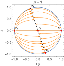
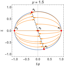
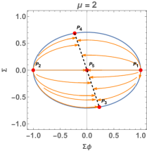
Figure 1: Phase Plot for system (68)-(69) for $\epsilon=+1$ and different values of $\mu$. The dashed black line corresponds to $L_{1}$.

In Fig. 1 is presented a phase plot for system (68)-(69) for $\epsilon=+1$ and different values of $\mu$. The dashed black line corresponds to $L_{1}$.

IV.1.2 Case $\epsilon=-1$

For the case $\epsilon=-1$, the equilibrium points of the system (68) and (69) are as before the line $L_{1}$ which contains $P_{5}$ (which does not satisfies (65). Moreover, imposing the condition (65), the lines are reduced to the points $P_{6}$ and $P_{7}$ that belongs to the lines of equilibrium points $3{\Sigma_{\phi}}+{\Sigma}=0$, where ${\Sigma_{\phi}}_{1,2}=\mp{1}/{\sqrt{9\mu-1}}$.

For these equilibrium points, we have $\dot{\phi}=\sqrt{6}{\Sigma_{\phi}}_{1,2}H$. Hence,

$$\dot{H}-{\Sigma_{\phi}}_{1,2}H\left(3{\Sigma_{\phi}}_{1,2}H+\sqrt{{\Lambda}/{(3\mu)}}\right)=0.$$ (74)

That is,

$$H=\frac{\sqrt{3}H_{0}\sqrt{\frac{\Lambda}{\mu}}}{\left(9H_{0}{\Sigma_{\phi}}_{1,2}+\sqrt{3}\sqrt{\frac{\Lambda}{\mu}}\right)e^{-(t-t_{U}){\Sigma_{\phi}}_{1,2}\sqrt{\frac{\Lambda}{3\mu}}}-9H_{0}{\Sigma_{\phi}}_{1,2}}.$$ (75)

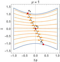
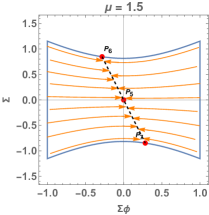
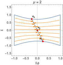
Figure 2: Phase plot for system (68) - (69) for $\epsilon=-1$ and different values of $\mu$. The dashed black line corresponds to $L_{1}$.

In Fig. 2 is presented a phase plot for system (68)-(69) for $\epsilon=-1$ and different values of $\mu$. The dashed black line corresponds to $L_{1}$.

IV.2 1D reduced system

Using (65) to reduce the dimensionality and for ${\Sigma}\geq 0$ we have

$${\Sigma}=\sqrt{(1-\Sigma_{\phi}^{2}\epsilon)/\mu}.$$ (76)

Then, we have the reduced dynamical system

$$\Sigma_{\phi}^{\prime}=-\left(3\Sigma_{\phi}+\sqrt{(1-\Sigma_{\phi}^{2}\epsilon)/\mu}\right)\left(1-\Sigma_{\phi}^{2}\epsilon\right),\$$ (77)

This patch cover only the equilibrium points (68)- (69) with $\Sigma>0$ and $\Sigma_{\phi}=0$, say, $P_{1}:\Sigma_{\phi}=1$, $P_{2}:\Sigma_{\phi}=-1$ and $P_{4}:\Sigma_{\phi}=-1/{\sqrt{9\mu+1}}$. Moreover, the equilibrium point of the 1D system (77) is $P_{6}:{\Sigma_{\phi}}=-{1}/{\sqrt{9\mu-1}}$.

Label	Existence	Coordinates  $\Sigma_{\phi}$	Eigenvalue	Stability
$P_{1,2}$	$\epsilon=+1$	$\pm 1$	6	Unstable
$P_{3}$	$\epsilon=+1,\mu>-\frac{1}{9}$	$\frac{1}{\sqrt{9\mu+1}}$	$-3$	Stable
$P_{6}$	$\epsilon=-1,\mu>\frac{1}{9}$	$-\frac{1}{\sqrt{9\mu-1}}$	$-3$	Stable

Table 2: Equilibrium points of system (77) for $\epsilon=\pm 1$ with their eigenvalues and stability

Tab. 2 presents the equilibrium points of system (77) for $\epsilon=\pm 1$ with their eigenvalues and stability.

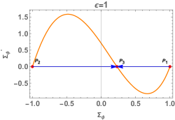
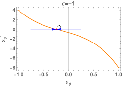
Figure 3: Phase plot for the reduced 1D equation (77) for $\epsilon=\pm 1$ and $\mu=2$.

In Fig. 3 is presented a phase plot for the reduced 1D equation (77) for $\epsilon=\pm 1$ and $\mu=2$.

On the other hand, using

$${\Sigma}=-\sqrt{(1-\Sigma_{\phi}^{2}\epsilon)/\mu},$$ (78)

we have the reduced dynamical system

$$\Sigma_{\phi}^{\prime}=-\left(3\Sigma_{\phi}-{\sqrt{(1-\Sigma_{\phi}^{2}\epsilon)/\mu}}\right)\left(1-\Sigma_{\phi}^{2}\epsilon\right),\$$ (79)

This patch cover only the equilibrium points (68)- (69) with $\Sigma<0$ and $\Sigma_{\phi}=0$, say, $P_{1}:\Sigma_{\phi}=1$ , $P_{2}:\Sigma_{\phi}=-1$ and $P_{3}:{\Sigma_{\phi}}:={1}/{\sqrt{9\mu+1}}$. Moreover, the equilibrium point of the 1D system (79) is $P_{7}:{\Sigma_{\phi}}={1}/{\sqrt{9\mu-1}}$, that belongs to the lines of equilibrium points $3{\Sigma_{\phi}}+{\Sigma}=0$.

Label	Existence	Coordinates  $\Sigma_{\phi}$	Eigenvalue	Stability
$P_{1,2}$	$\pm 1$	$\epsilon=+1$	6	Unstable
$P_{4}$	$\epsilon=+1,\mu>-\frac{1}{9}$	$-\frac{1}{\sqrt{9\mu+1}}$	$-3$	Stable
$P_{7}$	$\epsilon=-1,\mu>\frac{1}{9}$	$\frac{1}{\sqrt{9\mu-1}}$	$-3$	Stable

Table 3: Equilibrium points of system (79) for $\epsilon=\pm 1$ with their eigenvalues and stability

In Tab. 3 are presented the equilibrium points of system (79) for $\epsilon=\pm 1$ with their eigenvalues and stability.

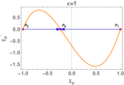
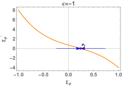
Figure 4: Phase plot for the reduced 1D equation (79) for $\epsilon=\pm 1$ and $\mu=2$.

Fig. 4 presents a phase plot for the reduced 1D equation (79) for $\epsilon=\pm 1$ and $\mu=2$.

V Dynamical systems analysis by including matter

We define

$${\Sigma_{\phi}}=\frac{\dot{\phi}}{\sqrt{6}H},\;{\Sigma}=\frac{\omega_{1}^{2}}{H},\;\Omega_{m}=\frac{\rho_{m}}{3H^{2}},$$ (80)

which satisfy

$${\Sigma_{\phi}}^{2}\epsilon+\mu{\Sigma}^{2}+\Omega_{m}=1.$$ (81)

V.1 3D system

The system (52), (53) and(52) can be written as the dynamical system given by

$${\Sigma_{\phi}}^{\prime}=\frac{3}{2}(w_{m}+1){\Sigma_{\phi}}\Omega_{m}+(3{\Sigma_{\phi}}+{\Sigma})\left({\Sigma_{\phi}}^{2}\epsilon-1\right),$$ (82)

$${\Sigma}^{\prime}=\frac{3}{2}(w_{m}+1){\Sigma}\Omega_{m}+{\Sigma_{\phi}}{\Sigma}\epsilon(3{\Sigma_{\phi}}+{\Sigma}),$$ (83)

$$\Omega_{m}^{\prime}=\Omega_{m}(3w_{m}(\Omega_{m}-1)+2{\Sigma_{\phi}}\epsilon(3{\Sigma_{\phi}}+{\Sigma})+3(\Omega_{m}-1)).$$ (84)

Label	Existence	Coordinates  $(\Sigma_{\phi},\Sigma,\Omega_{m})$	Eigenvalues	Stability
$P_{1,2}$	$\epsilon=+1$	$(\pm 1,0,0)$	$\{3,6,3(1-\omega_{m})\}$	Unstable
$L_{1}$	always	$(\Sigma_{\phi},-3\Sigma_{\phi},0)$	$\{-3,0,-3(\omega_{m}+1)\}$	Stable
$P_{3,6}$	$\epsilon=\pm 1$	$\left(\frac{\epsilon}{\sqrt{9\mu+\epsilon}},-\frac{3\epsilon}{\sqrt{9\mu+\epsilon}},0\right)$	$\{-3,0,-3(\omega_{m}+1)\}$	Stable
$P_{4,7}$	$\epsilon=\pm 1$	$\left(-\frac{\epsilon}{\sqrt{9\mu+\epsilon}},\frac{3\epsilon}{\sqrt{9\mu+\epsilon}},0\right)$	$\{-3,0,-3(\omega_{m}+1)\}$	Stable
$P_{5}$	$\nexists$	$(0,0,0)$	$\{-3,0,-3(\omega_{m}+1)\}$	Stable
$M$	$\epsilon=\pm 1$	$(0,0,1)$	$\left\{\frac{3(\omega_{m}-1)}{2},\frac{3(\omega_{m}+1)}{2},3(\omega_{m}+1)\right\}$	Stable for $\omega_{m}=-1$
				Unstable for $\omega_{m}=1$
				Saddle otherwise

Table 4: Equilibrium points of system (82), (83) and (84) for $\epsilon=\pm 1$ with their eigenvalues and stability

In Tab. 4 are presented the equilibrium points of system (82), (83) and (84) for $\epsilon=\pm 1$ with their eigenvalues and stability.

V.1.1 Case $\epsilon=+1$

For the case $\epsilon=+1$, the equilibrium points of the system (82), (83), and (84) are $P_{1}$, $P_{2}$ which are kinetic dominated solutions. The line of equilibrium points $L_{1}$ which represents de Sitter solutions. This line contains the points $P_{3}$, $P_{4}$ and $P_{5}$. Additionally, we have the matter-dominated solution $M:\left({\Sigma_{\phi}},{\Sigma},\Omega_{m}\right)=(0,0,1)$.

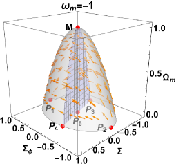
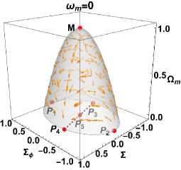
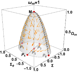
Figure 5: 3D phase plot for system (82), (83) and (84) for $\epsilon=+1$, $\mu=2$ and different values of $\omega_{m}$.

In Fig. 5 is presented a 3D phase plot for system (82), (83) and (84) for $\epsilon=1$, $\mu=2$ and different values of $\omega_{m}$.

V.1.2 Case $\epsilon=-1$

For the case $\epsilon=-1$, the equilibrium points of the system (82), (83), and (84) are the line of equilibrium points $L_{1}$ which represents de Sitter solutions. This line contains the points $P_{5}$, $P_{6}$ and $P_{7}$. Additionally, we have the matter-dominated solution $M:\left({\Sigma_{\phi}},{\Sigma},\Omega_{m}\right)=(0,0,1)$.

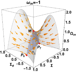
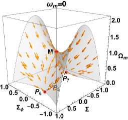
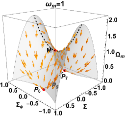
Figure 6: 3D phase plot for system (82), (83) and (84) for $\epsilon=-1$, $\mu=2$ and different values of $\omega_{m}$.

In Fig. 6 is presented a 3D phase plot for system (82), (83) and (84) for $\epsilon=-1$, $\mu=2$ and different values of $\omega_{m}$.

V.2 Reduced 2D system

Eliminating $\Omega_{m}$ from (81) to obtain the reduced system 

$${\Sigma_{\phi}}^{\prime}=-\frac{1}{2}\left({\Sigma_{\phi}}^{2}\epsilon-1\right)(3(w_{m}-1){\Sigma_{\phi}}-2{\Sigma})-\frac{3}{2}\mu(w_{m}+1){\Sigma_{\phi}}{\Sigma}^{2},$$ (85)

$${\Sigma}^{\prime}=\frac{3}{2}(w_{m}+1){\Sigma}\left(1-{\Sigma_{\phi}}^{2}\epsilon-\mu{\Sigma}^{2}\right)+{\Sigma_{\phi}}{\Sigma}\epsilon(3{\Sigma_{\phi}}+{\Sigma}).$$ (86)

V.2.1 Case $\epsilon=+1$

The equilibrium points of the system (85) and (86) are $P_{1,2}$ $L_{1}$, $P_{3}$, $P_{4}$ and $M$, summarised in Tab. 5.

Label	Coordinates  $(\Sigma_{\phi},\Sigma)$	Eigenvalues	Stability
$P_{1,2}$	$(\pm 1,0)$	$\{3,6\}$	Unstable
$L_{1}$	$(\Sigma_{\phi},-3\Sigma_{\phi})$	$\{-3,-3(\omega+1)\}$	Stable
$P_{3}$	$\left(\frac{1}{\sqrt{9\mu+1}},-\frac{3}{\sqrt{9\mu+1}}\right)$	$\{-3,-3(\omega+1)\}$	Stable
$P_{4}$	$\left(-\frac{1}{\sqrt{9\mu+1}},\frac{3}{\sqrt{9\mu+1}}\right)$	$\{-3,-3(\omega+1)\}$	Stable
$M$	$(0,0)$	$\left\{\frac{3(\omega_{m}-1)}{2},3(\omega_{m}+1)\right\}$	Stable for $\omega=-1$
			Unstable for $\omega=1$
			Saddle otherwise

Table 5: Equilibrium points of system (85) and (86) for $\epsilon=+1$ with their eigenvalues and stability

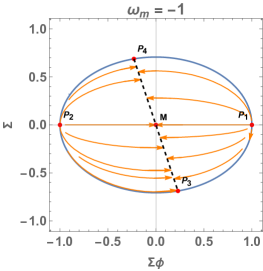
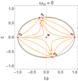
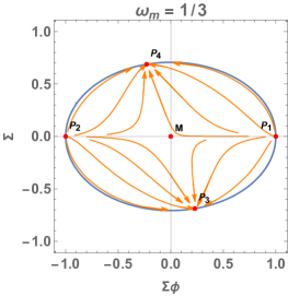
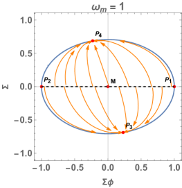
Figure 7: 2D projections of the system (85)-(86) for $\epsilon=+1$, $\mu=2$ and different values of $\omega_{m}$.

In Fig. 7 are presented 2D projections of the system (85)-(86) for $\epsilon=+1$, $\mu=2$ and different values of $\omega_{m}$.

V.2.2 Case $\epsilon=-1$

The equilibrium points of the system (85) and (86) for $\epsilon=-1$ are summarised in Tab. 6.

Label	Coordinates  $(\Sigma_{\phi},\Sigma)$	Eigenvalues	Stability
$L_{1}$	$(\Sigma_{\phi},-3\Sigma_{\phi})$	$\{-3,-3(\omega_{m}+1)\}$	Stable
$P_{6}$	$\left(\frac{1}{\sqrt{9\mu-1}},-\frac{3}{\sqrt{9\mu-1}}\right)$	$\{-3,-3(\omega+1)\}$	Stable
$P_{7}$	$\left(-\frac{1}{\sqrt{9\mu-1}},\frac{3}{\sqrt{9\mu-1}}\right)$	$\{-3,-3(\omega+1)\}$	Stable
$M$	$(0,0)$	$\left\{\frac{3(\omega_{m}-1)}{2},3(\omega_{m}+1)\right\}$	Stable for $\omega=-1$
			Unstable for $\omega=1$
			Saddle otherwise

Table 6: Equilibrium points of system (85) and (86) for $\epsilon=-1$ with their eigenvalues and stability.

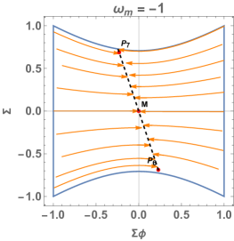
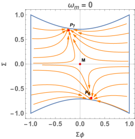
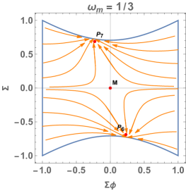
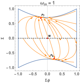
Figure 8: 2D projection (85)-(86) for $\epsilon=-1$, $\mu=2$ and different values of $\omega_{m}$.

In Fig. 8 is presented a 2D projection (85)-(86) for $\epsilon=-1$, $\mu=2$ and different values of $\omega_{m}$.

VI Conclusions

In this study, we investigated the effects of the modification of the Poisson algebra on the dynamics of scalar field cosmology. Specifically, we performed a detailed analysis of the phase-space by studying the equilibrium points and their stability, such that, reconstructing the cosmological history.

The modified Poisson algebra modifies the field equations such that a cosmological constant term is introduced and the pressure component of the scalar field’s energy-momentum tensor is different from that of the canonical scalar field. Moreover, a mass term for the scalar field is introduced, which is described by the cosmological constant.

As a result, the equilibrium points provided by the modified field equations are different from that of the usual scalar field model. From the analysis, we can conclude that the modified equations can provide more than one accelerated universe, described by the de Sitter solution. Hence, cosmic inflation and late-time acceleration are provided by the specific theory.

In the matter-less case, we divided the study into two subcases, one for $\epsilon=1$ and one for $\epsilon=-1$. In total, we have six families of physically accepted equilibrium points which can describe stiff fluid solutions and de Sitter spacetime in the asymptotic regime.

In the case with the matter, we also consider the subcases $\epsilon=\pm 1,$ and in total, we obtained eight families of equilibrium points, the same ones as in the case without matter and just one additional equilibrium point which describes matter.

In future work, we plan to investigate further the modified field equations with the introduction of a nonzero scalar field potential, while an interacting term between the scalar field and the matter source will be considered.

References

- (1) M. Tegmark et al., Astrophys. J. 606 (2004) 702
- (2) M. Kowalski et al., Astrophys. J. 686 (2008) 749
- (3) E. Komatsu et al., Astrophys. J. Suppl. Ser. 180, 330 (2009)
- (4) P.A.R. Ade, Astron. Astroph. 571 (2014) A15
- (5) T. Padmanabhan, Phys. Rept. 380 (2003) 235
- (6) S. Weinberg, Rev. Mod. Phys. 61 (1989) 1
- (7) E. Di Valentino, O. Mena, S. Pan, L. Visinelli, W. Yang, A. Melchiorri, D.F. Mota, A.G. Reiss and J. Silk, In the Realm of the Hubble tension - a Review of Solutions, Class. Quantum Grav. 38, 153001 (2021)
- (8) B. Ratra and P. J. E. Peebles, Phys. Rev D., 37, 3406 (1988).
- (9) W. Chen and Y-S. Wu, Phys. Rev. D 41, 695 (1990);
- (10) S. Basilakos, M. Plionis and S. Solà, Phys. Rev. D. 80, 3511 (2009).
- (11) C. Wetterich, Astron. Astrophys. 301, 321 (1995)
- (12) R. R. Caldwell, R. Dave, and P.J. Steinhardt, Phys. Rev. Lett., 80, 1582 (1998).
- (13) P. Brax, and J. Martin, Phys. Lett. B468, 40 (1999).
- (14) R. R. Caldwell, Phys. Rev. Lett. B., 545, 23 (2002).
- (15) J. A. S. Lima, F. E. Silva and R. C. Santos, Class. Quant. Grav. 25, 205006 (2008), arXiv:0807.3379 [astro-ph].
- (16) A. W. Brookfield, C. van de Bruck, D.F. Mota, and D. Tocchini-Valentini, Phys. Rev. Lett. 96, 061301 (2006).
- (17) L. Amendola and S. Tsujikawa, Dark Energy Theory and Observations, Cambridge University Press, Cambridge, England, (2010)
- (18) A.A. Starobinsky, Phys. Lett. B 91, 99 (1980)
- (19) A. Guth, Phys. Rev. D 23, 347 (1981)
- (20) A.D. Linde, Phys. Lett. B 129, 177 (1983)
- (21) A.R. Liddle, Phys. Lett. B 220, 502 (1989)
- (22) T. Charters, J.P. Mimoso and A. Nunes, Phys. Lett. B 472, 21 (2000)
- (23) J.D. Barrow and P. Saich, Class. Quantum Grav. 10, 279 (1993)
- (24) S.V. Chervon, V.M. Zhuravlev and V.K. Shchigolev, Phys. Lett. B 398, 269 (1997)
- (25) R. Kallosh and A. Linde, JCAP 13, 027 (2013)
- (26) A. Paliathanasis, Mod. Phys. Lett. A 37, 2250119 (2022)
- (27) J. de Haro, J. Amorós and S. Pan, Phys. Rev. D 93, 084018 (2016)
- (28) A.D. Dolgov, in: The very Early Universe, Ed. G. Gibbons, S.W. Hawking, S.T. Tiklos (Cambridge U., 1982)
- (29) H. K. Jassal, J.S. Bagla, T. Padmanabhan, Phys. Rev. D72 103503, (2005); H.K. Jassal, J.S. Bagla, T. Padmanabhan, Mon. Not. Roy. Astron. Soc. Letters 356, L11-L16, (2005)
- (30) L. Samushia, B. Ratra, Astrophys. J. 650, L5, (2006); Astrophys. J. 680, L1, (2008)
- (31) J. Simon, L. Verde, R. Jiménez, Phys. Rev. D71, 123001, (2005)
- (32) J.D. Barrow and A. Paliathanasis, Phys. Rev. D 94, 083518 (2016)
- (33) S. Pan, W. Yang and A. Paliathanasis, EPJC 80, 274 (2020)
- (34) V. Faraoni, Int. J. Mod. Phys. D 11, 471 (2002)
- (35) J. A. S. Lima and J. S. Alcaniz, Phys. Lett. B 600, 191 (2004)
- (36) S. H. Pereira and J. A. S. Lima, Phys. Lett. B 669, 266 (2008)
- (37) A. Paliathanasis, M. Tsamparlis and S. Basilakos, Phys. Rev. D 90, 103524 (2014)
- (38) J. Martin and R. H. Brandenberger, Phys. Rev. D 63, 123501 (2001)
- (39) J. C. Niemeyer, Phys. Rev. D 63, 123502 (2001).
- (40) A. Kempf, Phys. Rev. D 63, 083514 (2001), astro-ph/0009209.
- (41) A. Kempf and J. Niemeyer, Phys. Rev. D 64, 103501 (2001).
- (42) A. Ashoorioon, A. Kempf and R.B. Mann, Phys. Rev. D 71, 023503 (2005).
- (43) A. Ashoorioon, J. L. Hovdebo and R. B. Mann, Nucl. Phys. B 727, 63-76 (2005)
- (44) A. Zampeli and A. Paliathanasis, Class. Quantum Grav. 38, 165012 (2021)
- (45) A. Paliathanasis, Universe 7, 52 (2021)
- (46) A. Zampeli, T. Pailas, P.A. Terzis and T. Christodoulakis, JCAP 05, 066 (2016)
- (47) S. Mukhi, Class. Quant. Grav. 28, 153001 (2011).
- (48) J. Kowalski-Glikman, Lect. Notes Phys. 669, 131-159 (2005).
- (49) G. Amelino-Camelia, Symmetry 2, 230-271 (2010).
- (50) J. D. Bekenstein, Phys. Rev. D 7, 2333 (1973).
- (51) J. D. Bekenstein, Letter Nuovo Cimento 4, 737 (1972).
- (52) M. Maggiore, Phys. Lett. B 304, 65 (1993).
- (53) A. Giacomini, G. Leon, A. Paliathanasis and S. Pan, Eur. Phys. J. C 80 (2020) no.10, 931
- (54) A. Paliathanasis, G. Leon, W. Khyllep, J. Dutta and S. Pan, Eur. Phys. J. C 81 (2021) no.7, 607
- (55) S. Masood, M. Faizal, Z. Zal, A.F. Ali, J. Raza and M.B. Shah, Phys. Lett. B 763, 218 (2016)
- (56) S. Pérez-Payán, M. Sabido and C. Yee-Romero, Phys. Rev. D 88 (2013) no.2, 027503
- (57) B. Tajahmad, EPJC 82, 965 (2022)
- (58) P. G. N. de Vegvar, Eur. Phys. J. C 81 (2021) no.9, 786
- (59) S. Basilakos, M. Tsamparlis and A. Paliathanasis, Phys. Rev. D 83 (2011), 103512
- (60) A. Paliathanasis and M. Tsamparlis, Phys. Rev. D 90 (2014) no.4, 043529
- (61) A. Paliathanasis, G. Leon and S. Pan, Gen. Rel. Grav. 51 (2019) no.9, 106
- (62) A. B. Burd and John D. Barrow. Nucl. Phys. B, 308:929–945, 1988. [Erratum: Nucl.Phys.B 324, 276–276 (1989)].
- (63) R. Tavakol. Introduction to dynamical systems, page 84–104. Cambridge University Press, 1997.
- (64) Edmund J. Copeland, Andrew R Liddle, and David Wands. Phys. Rev. D, 57:4686–4690, 1998.
- (65) A. A. Coley. Dynamical systems and cosmology. Kluwer, Dordrecht, Netherlands, 2003.
- (66) Genly Leon and Carlos R. Fadragas. Cosmological dynamical systems. Saarbrücken, Germany, 2012. LAP LAMBERT Academic Publishing. ISBN 978-3-8473-0233-9.
- (67) Yungui Gong, Anzhong Wang, and Yuan-Zhong Zhang. Phys. Lett. B, 636:286–292, 2006.
- (68) M. R. Setare and E. N. Saridakis. Phys. Rev. D, 79:043005, 2009.
- (69) Xi-ming Chen, Yun-gui Gong, and Emmanuel N. Saridakis. JCAP, 04:001, 2009.
- (70) Gaveshna Gupta, Emmanuel N. Saridakis, and Anjan A. Sen. Phys. Rev. D, 79:123013, 2009.
- (71) H. Farajollahi, A. Salehi, F. Tayebi, and A. Ravanpak. JCAP, 05:017, 2011.
- (72) L. Arturo Urena-Lopez. JCAP, 03:035, 2012.
- (73) Dagoberto Escobar, Carlos R. Fadragas, Genly Leon, and Yoelsy Leyva. Class. Quant. Grav., 29:175005, 2012.
- (74) Dagoberto Escobar, Carlos R. Fadragas, Genly Leon, and Yoelsy Leyva. Class. Quant. Grav., 29: 175006, 2012.
- (75) Chen Xu, Emmanuel N. Saridakis, and Genly Leon. JCAP, 07:005, 2012.
- (76) Genly Leon, Joel Saavedra, and Emmanuel N. Saridakis. Class. Quant. Grav., 30:135001, 2013.