U-Flow: A U-shaped Normalizing Flow for Anomaly Detection with Unsupervised Threshold^*

Abstract

In this work we propose a non-contrastive method for anomaly detection and segmentation in images, that benefits both from a modern machine learning approach and a more classic statistical detection theory. The method consists of three phases. First, features are extracted using a multi-scale image Transformer architecture. Then, these features are fed into a U-shaped Normalizing Flow that lays the theoretical foundations for the last phase, which computes a pixel-level anomaly map, and performs a segmentation based on the a contrario framework. This multiple-hypothesis testing strategy permits to derive robust automatic detection thresholds, which are crucial in many real-world applications, where an operational point is needed. The segmentation results are evaluated using the Intersection over Union (IoU) metric; and for assessing the generated anomaly maps we report the area under the Receiver Operating Characteristic curve (AUROC), and the area under the per-region-overlap curve (AUPRO). Extensive experimentation in various datasets shows that the proposed approach produces state-of-the-art results for all metrics and all datasets, ranking first in most MvTec-AD categories, with a mean pixel-level AUROC of 98.74%.

Code and trained models are available at https://github.com/mtailanian/uflow.

1 Introduction

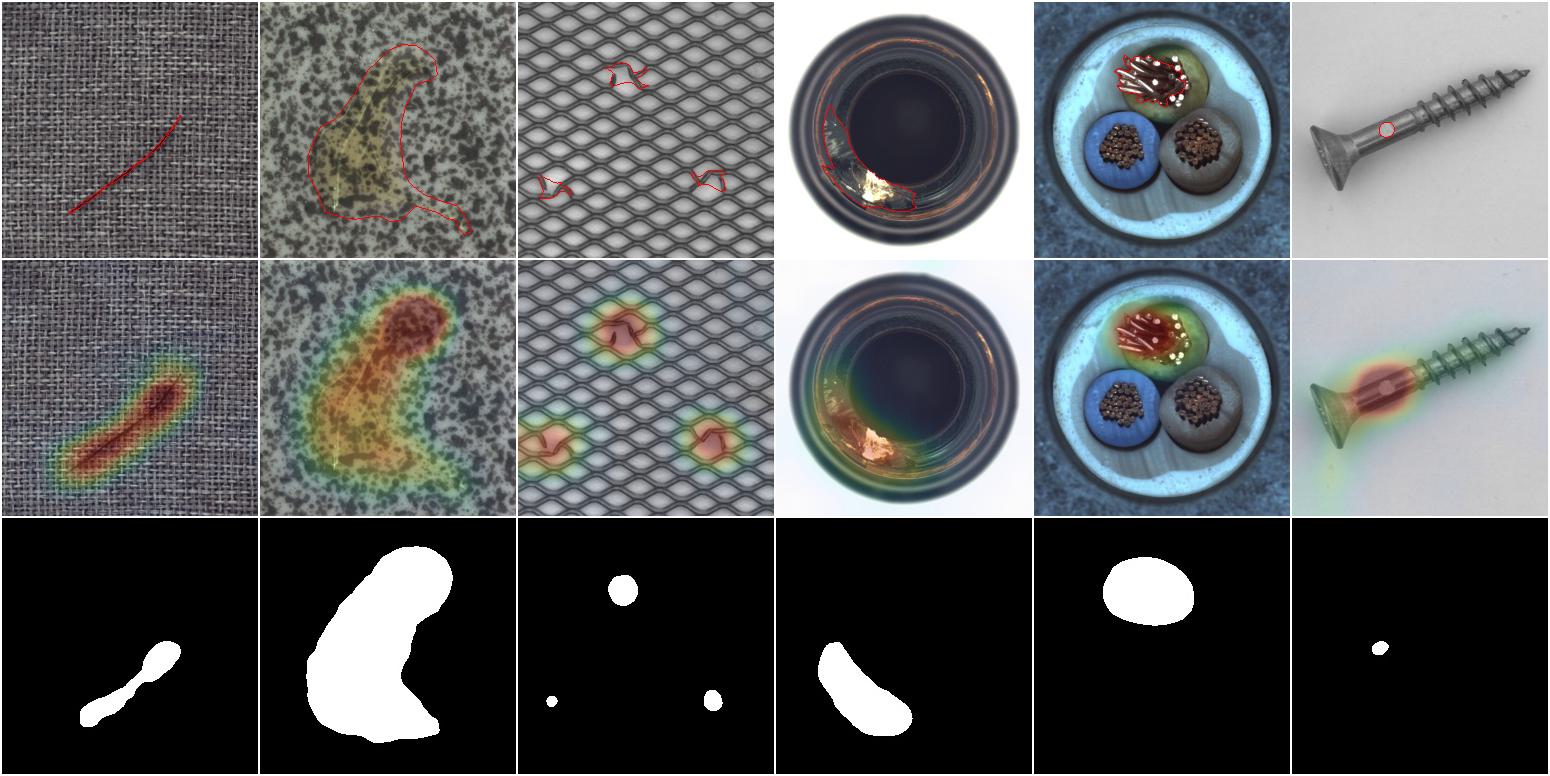
Figure 1: Anomalies detected with the proposed approach, on MvTec-AD examples from different categories. Top row: original images with ground truth segmentation. Middle and bottom rows: corresponding anomaly maps and automatic segmentations.

The detection of anomalies in images is a long-standing problem that has been studied for decades. In recent years this problem has received a growing interest from the computer vision community, motivated by applications in a wide range of fields, ranging from surveillance and security to even health care. But one of the most common applications, and the one that we are especially interested in, is automatizing product quality control in an industrial environment. In this case, it is often very hard (or sometimes even infeasible) to collect and label a good amount of data with a representation of all kinds of anomalies, since by definition these are rare structures. For this reason, the major effort on anomaly detection methods has been focused on unsupervised and self-supervised non-contrastive learning, where only normal samples (i.e. anomaly-free images) are required for training.

Currently, the most common approach for anomaly detection consists in embedding the training images in some latent space, and then evaluating how far a test image is from the manifold of normal images [4, 5, 34, 41, 27, 19].

Other approaches focus on learning the probability density function of the training set. Among these, three types of generative models became popular in anomaly detection in the last five years. On one hand, Generative Adversarial Networks [13, 30] learn this probability in an implicit way, being able only to sample from it. On the other hand, Variational Auto-Encoders [18, 40] are capable of explicitly estimating this probability density, but they can only learn an approximation, as they maximize the evidence lower bound. And finally, Normalizing Flows [7, 8, 17] are able to explicitly learn the exact probability density function. Being able to do so has several advantages, as it permits to estimate the likelihood and score how probable it is that the tested data belongs to the same training distribution. A major advantage, that we exploit in this work, is the possibility to develop formal statistical tests to derive unsupervised detection thresholds. This is a crucial feature for most real-world problems, where a segmentation of the anomaly is needed. To this end, we propose a multiple-hypothesis testing strategy based on the a contrario framework [6].

In this work we propose U-Flow, a new self-supervised non-contrastive method that ensembles the features extracted by multi-scale image transformers into a U-shaped Normalizing Flow’s architecture, and applies the a contrario methodology for finding an automatic segmentation of anomalies in images. Our work achieves state-of-the-art results, widely outperforming previous works in terms of IoU for the segmentation, and exhibiting top performance in localization metrics in terms of AUROC and AUPRO. The main contributions of this paper are:

• For the feature extraction, we propose a multi-scale vision Transformer architecture based on the CaiT Transformer [33], which we refer to as MS-CaiT. Although the different scales are combined following a simple strategy based on a U-Net, results clearly show that it better captures the multi-scale information, and increases performance.

• We leverage the well-known advantages of U-like architectures in the setting of Normalizing Flows (NF), proposing a novel architecture and solving non-trivial technical details for merging the scales in an invertible way, that better aggregates the multi-scale information while imposing statistical mutual independence within and across scales.

• The resulting multi-scale characterization of the anomaly-free images as a white Gaussian process in the latent space, allows us to propose a multiple-hypothesis testing strategy that leads to an automatic detection threshold to segment anomalies, outperforming state-of-the-art methods.

In short, we propose an easy-to-train method, that does not require any parameter tuning or modification to the architecture (as opposed to other state-of-the-art methods), that is fast, accurate, and provides an unsupervised anomaly segmentation. Example results are shown in Figure 1.

The remainder of this paper is organized as follows. In Section 2 we discuss previous work related to the proposed approach. Details of the method are presented in Section 3. In Section 4 we compare the performance of our anomaly detection approach with a large number of state-of-the-art methods, on several benchmark datasets of different nature: MVTec-AD [2], BeanTech [24], LGG MRI [3], and ShanghaiTech Campus [22]. An ablation study, that analyzes the role of each component of the proposed architecture, is presented in Section 5. We conclude in Section 6.

2 Related work

The literature on anomaly detection is very extensive, and many approaches have been proposed. In this work, we focus on non-contrastive self-supervised learning, where the key element is to learn only from anomaly-free images. Within this group, methods can be further divided into several categories.

Representation-based methods proceed by embedding samples into a latent space and measuring some distance between them. For example in CFA [19], the authors propose a method to build features using a patch descriptor, and building a scalable memory bank. A special loss function is designed to map features to a hyper-sphere and densely clusterize the representation of normal images. Also, the method has the possibility of adding a few abnormal samples during training, that are used to enlarge the distance to the normal samples in the latent space. Similarly, in [41], the authors also construct a hierarchical encoding of image patches and encourage the network to map them to the center of a hyper-sphere in the feature space. This work later inspired [34], where the authors aim to learn more representative features from normal images, using three encoders with three classifiers. In SPADE [4] the anomaly score is obtained by measuring the distance of a test sample to the nearest neighbors that were computed at the training stage over the anomaly-free images. Additionally, PaDiM [5] proposes to model normality by fitting a multivariate Gaussian distribution after embedding image patches with a pre-trained CNN, and base the detection on the Mahalanobis distance to the normality. Then, PatchCore [27] further improves SPADE and PaDiM, by estimating anomalies with a larger nominal context and making it less reliant on image alignment.

Reconstruction-based methods ground anomaly detection in the analysis of the reconstruction error. By using an encoder-decoder architecture such as [40], or a teacher-student scheme like [39], and training the network with only anomaly-free images, the network is supposed to accurately reconstruct normal images, but fail to reconstruct anomalies, as it has never seen them. Learning from one-class data leaves some uncertainty on how the network will behave for anomalous data. To overcome this potential issue, some works manage to convert the problem into a self-supervised one, by creating some proxy task. For example in [20], authors obtain a representation of the images by randomly cutting and pasting regions over anomaly-free images to synthetically generate anomalies.

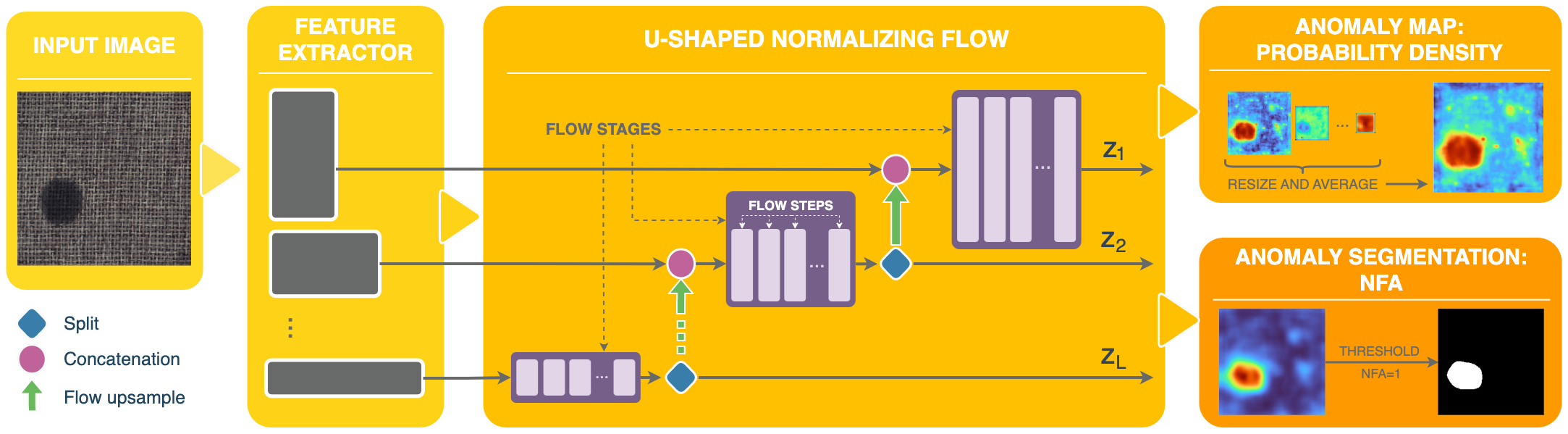
Figure 2: The method consists of three phases. (1) Multi-scale feature extraction: a rich multi-scale representation is obtained with MS-CaiT, by combining pre-trained image Transformers acting at different image scales. (2) U-shaped Normalizing Flow: by adapting the widely used U-like architecture to NFs, a fully invertible architecture is designed. This architecture is capable of merging the information from different scales while ensuring independence both intra- and inter-scales. To make it fully invertible, split and invertible up-sampling operations are used. (3) Anomaly score and segmentation computation: besides generating the anomaly map based on the likelihood of test data, we also propose to adapt the a contrario framework to obtain an automatic threshold by controlling the allowed number of false alarms.

Regarding the use of Normalizing Flows in anomaly detection, a few methods have been recently proposed [28, 42, 14], among which CFlow [14] and FastFlow [42] stand out for their impressive results. The former uses a one-dimensional NF and include the spatial information using a positional encoding as a conditional vector, while the latter directly uses a two-dimensional NF. In both cases, an anomaly score is then computed based on the likelihood estimation of test data. In this work, we further improve the performance of these methods, by proposing a multi-scale Transformer-based feature extractor, and by equipping the NFs with a fully invertible U-shaped architecture. These two ingredients allow us to embed these multi-scale features in a latent space where intra and inter-scale features are guaranteed to be independent and identically distributed Gaussian random variables. From these statistical properties, we can easily design a detection methodology that leads to statistically meaningful anomaly scores and unsupervised detection thresholds.

3 Method

The proposed method is depicted in Figure 2, and consists of three main phases: 1) Feature extraction, 2) U-shaped Normalizing Flow, and 3) Anomaly score and segmentation. The three phases are presented in the following.

3.1 Phase 1: Feature extraction

Due to the fact that anomalies can emerge in a variety of sizes and forms, it is essential to collect image information at multiple scales. To do so, the standard deep learning strategy is to use pre-trained CNNs, often a VGG [31] or any variant of the ResNet [15] architectures, to extract a rich multi-scale image feature representation, by keeping the intermediate activation maps at different depths of the network. More recently, with the development of image vision Transformers, some architectures such as ViT [9] and CaIT [33] are also being used, but in these cases, a single feature map is retrieved. The features generated by vision Transformers are proven to better compress all multi-scale information into a single feature map volume, compared to the standard CNNs. However, this notion of a unique multi-scale feature map was challenged by MViT [11], which proved that combining the standard CNNs’ idea of having multi-scale feature hierarchies with the Transformer models, the Transformers’ features could be further enhanced. This work was followed by MViT2 [21], which later showed to outperform its predecessor and all other vision Transformers in various tasks. In our work, we also propose to construct a multi-scale Transformer architecture but following a different strategy. More specifically, we propose MS-CaiT; an architecture that employs two CaIT Transformers at different scales, independently pre-trained on ImageNet [29], and combines them as the encoder of a U-Net [26] architecture. Despite its simplicity, an ablation study presented in Section 5.2 shows that this combination strategy leads to better results than using each one of the Transformers alone, far better than other ResNet variants, and even better than MViT2. We conjecture that the fact that both CaIT networks were trained independently could be somehow beneficial, in the sense that it might give the network more flexibility to concentrate on different structures in each Transformer.

As a final comment regarding the feature extraction stage, it is important to mention that, although the proposed architecture is presented as agnostic to the feature extractor, all the results reported in Section 4 were obtained using the exact same architecture configuration.

3.2 Phase 2: Normalizing Flow

The rationale for using NFs in an anomaly detection setting is straightforward. The network is trained using only anomaly-free images, and in this way it learns to transform the distribution of normal images into a white Gaussian noise process. At test time, when the network is fed with an anomalous image, it is expected that it will not generate a sample with a high likelihood according to the white Gaussian noise model. Hence, a low likelihood indicates the presence of an anomaly.

This second phase is the only one that is trained. It takes as input the multi-scale representation generated by the feature extractor, and performs a sequence of invertible transformations on the data, using the NF framework.

State-of-the-art methods following this approach are centered on designing or trying out different existent multi-scale feature extractors. In this work, we further improve the approach by not only proposing a new feature extractor, but also a multi-level deep feature integration method, that aggregates the information from different scales using the well-known and widely used UNet-like [26] architecture. The U-shape is composed of the feature extractor as the encoder and the NF as the decoder. We show in the ablation study of Section 5.1 that the U-shape is a beneficial aggregation strategy and further improves the results.

The NF in this phase uses only invertible operations, and it is implemented as one unique graph, therefore obtaining a fully invertible network. Optimizing the whole flow all at once has a crucial implication: the Normalizing Flow generates an embedding that is mutually independent not only inside each scale but also inter-scales, unlike CFlow [14] and FastFlow [42]. Although this independence is theoretically guaranteed by NFs, due to the training process involved, it might be the case where the independence does not actually stand. To test it, we experimented with adding a term to the loss function in the training process, based on the Gram matrices of all scales. In practice, we obtained the same results and checked that the matrices were actually diagonal during the whole training, even when not using the mentioned loss term. It is worth mentioning that in all works reported so far in the literature, the anomaly score is computed first at each scale independently, using a likelihood-based estimation, and finally merged by averaging or summing the result for each scale. Because of the lack of independence between scales, these final operations, although achieving very good performance, lack of a formal probabilistic interpretation. The NF architecture proposed in this work overcomes this limitation; indeed, it produces statistically independent multi-scale features, for which the joint likelihood estimation becomes trivial.

Architecture. The U-shaped NF is compounded by a number of flow stages, each one corresponding to a different scale, whose size matches the extracted feature maps (see Figure 2). For each scale starting from the bottom, i.e. the coarsest scale, the input is fed into its corresponding flow stage, which is essentially a sequential concatenation of flow steps. The output of this flow stage is then split in such a way that half of the channels are sent directly to the output of the whole graph, and the other half is up-sampled, to be concatenated with the input of the next scale, and proceed in the same fashion. The up-sampling is also performed in an invertible way, as proposed in [16], where pixels in groups of four channels are reordered in such a way that the output volume has 4 times fewer channels, and double width and height.

Each flow step has a size according to its scale, and is compounded by Glow blocks [17]. Each step combines an Affine Coupling layer [7], a permutation using $1\times 1$ convolutions, and a global affine transformation (ActNorm) [8]. The Affine Coupling layer uses a small network with the following layers: a convolution, a ReLU activation, and one more convolution. Convolutions have the same amount of filters as the input channels, and kernels alternate between $1\times 1$ and $3\times 3$.

To sum up, the U-shaped NF produces $L$ white Gaussian embeddings $z_{1},\dots,z_{L}$, one for each scale $l$, $z^{l}\in\mathbb{R}^{C_{l}\times H_{l}\times W_{l}}$. Here we denote by $(i,j)$ a pixel location in the input image, and by $k$ the channel index in the latent tensor. Its elements $z_{ijk}^{l}~{}\sim~{}\mathcal{N}(0,1)$, $1\leq i\leq H_{l}$, $1\leq j\leq W_{l}$, $1\leq k\leq C_{l}$, are mutually independent for any position, channel and scale $i,j,k,l$.

3.3 Phase 3: Anomaly score and segmentation

The last phase of the method is to be used at test time when computing the anomaly map and its corresponding segmentation. Thanks to the statistical independence of the features produced by the U-shaped NF, the joint likelihood of a test image under the anomaly-free image model is the product of the standard normal marginals.

More precisely, this third and last phase of our method produces two outputs (see Figure 2), described below.

3.3.1 Likelihood-based Anomaly Score

The first output is an anomaly map that associates to each pixel $(i,j)$ in the test image, the same likelihood-based Anomaly Score proposed in FastFlow and CFlow,

$$AS_{ij}=-\frac{1}{L}\sum_{l=1}^{L}\exp\left(-\frac{1}{2}\frac{1}{C_{l}}\sum_{k=1}^{C_{l}}\frac{1}{2}(z_{ijk}^{l})^{2}\right).$$ (1)

Note that this score does not correspond exactly to the anomaly-free likelihood, mainly since it averages the (unnormalized) likelihood of each scale, instead of computing their product. This of course lacks of a clear probabilistic interpretation, but produces high quality anomaly maps and allows us to compare our approach to other state-of-the-art methods.

In order to obtain a more formal and statistically meaningful result, the output of this third phase produces also a second anomaly score called Number of False Alarms (NFA), computed following the a contrario framework. Moreover, this framework permits to derive an unsupervised detection threshold on the NFA, that produces an anomaly segmentation mask.

3.3.2 NFA: Number of False Alarms

The a contrario framework [6] is a multiple-hypothesis testing methodology that has been successfully applied to a wide variety of detection problems, such as alignments for line segment detection [36], image forgery detection [12], and even anomaly detection [32], to name a few. It is based on the non-accidentalness principle [23]. Given the fact that we do not usually know what the anomalies look like, it focuses on modeling normality, by defining a null hypothesis ($\mathcal{H}_{0}$), also called background model. Relevant structures are detected as large deviations from this model, by evaluating how likely it is that an observed structure or event $E$ would happen under $\mathcal{H}_{0}$. One of its most useful characteristics is that it provides an easily interpretable detection threshold based on controlling the NFA, defined as

$$\text{NFA}(E)=N_{T}\mathrm{P_{\mathcal{H}_{0}}}(E).$$ (2)

Here $N_{T}$ denotes the number of events that are tested, and $\mathrm{P_{\mathcal{H}_{0}}}(E)$ (also noted just as $P$ in the following), is the probability of the event $E$ to happen as a realization of the background model. Besides providing a robust detection threshold, as it will be shown, the NFA value itself has a clear statistical meaning: it is an estimate of the number of times, among the tests that are performed, that such tested event could be generated by the background model. In other words, $NFA(E)\leq\epsilon$ means that at most $\epsilon$ events like $E$ could happen by chance under the normality assumption. Hence, a low NFA value means that the observed pattern is too unlikely to be generated by the background model, and therefore indicates a meaningful anomaly.

In our anomaly detection setting, as the embedding produced by the U-Flow is $z_{ijk}^{l}~{}\sim~{}\mathcal{N}(0,1),\text{i.i.d.}$, we characterize normality by defining a background model on $(z_{ijk}^{l})^{2}$ to follow a Chi-Squared distribution of order 1,

$$(z_{ijk}^{l})^{2}\sim\mathcal{X}^{2}(1)\;\;\text{i.i.d.}$$ (3)

Then, instead of basing the criterion only on the observed pixel, we consider a block $B_{ij}^{l}$ of size $w_{l}\times w_{l}\times C_{l}$ centered on pixel $(i,j)$ and spreading through all channels, as shown in Figure 3, and define a set of candidates $\mathcal{S}^{B_{ij}^{l}}$ as the voxels inside the block with suspiciously high values, according to our normality assumption given by (3):

$$\mathcal{S}^{B_{ij}^{l}}=\{(i^{\prime},j^{\prime},k)\;/\;(z^{l}_{i^{\prime}j^{\prime}k})^{2}>\tau\},$$ (4)

with $i^{\prime}\in[i-w_{l}/2,i+w_{l}/2]$, $j^{\prime}\in[j-w_{l}/2,j+w_{l}/2]$, $k\in[1,C_{l}]$, and $\tau$ fixed to represent a $p$-value of $p=0.9$ in the $\mathcal{X}^{2}(1)$ distribution.

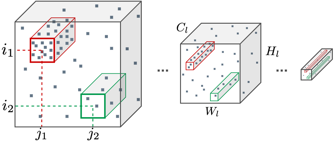
Figure 3: Tested regions for the NFA computation. Detection is based on the concentration of candidates, marked as gray solid points inside the volumes (the outputs of the NF phase). Blocks in red ($B_{i_{1}j_{1}}^{l}$) represent an anomalous region, while blocks in green ($B_{i_{2}j_{2}}^{l}$) represent a normal concentration of candidates.

Under the normality assumption, all such candidates are uniformly distributed. As anomalies usually appear in the image as connected components, we base our approach on detecting conspicuous concentrations of these candidate voxels. Given an observed number $|\mathcal{S}^{B_{ij}^{l}}|$ of such points within $B_{ij}^{l}$, the probability that the background model produces at least this number of such points within $B_{ij}^{l}$, which we denote by $P_{ij}^{l}$, is given by the tail of the Binomial distribution, i.e. $P_{ij}^{l}=\mathcal{B}\left(|\mathcal{S}^{B_{ij}^{l}}|,w_{l}^{2}C_{l},1-p\right)$. However, as the number of voxels in the block $B_{ij}^{l}$ is usually too high ($w_{l}^{2}C_{l}$), the Binomial distribution values become too small and usually conduct to numerical instabilities. To remediate this fact and to obtain a more robust estimation, we reduce this number of voxels by instead considering average numbers per channel. More precisely, for each tested block, we evaluate the probability, under the background model, of the average number per channel of candidate voxels being larger than the observed one:

$$P_{ij}^{l}=\mathcal{B}\left(|\mathcal{S}^{B_{ij}^{l}}|/C_{l},w_{l}^{2},1-p\right).$$ (5)

Finally, thanks to the independence between scales resulting from the NF, the probability estimates for joint scales can be computed as

$$P_{ij}=\prod_{l=1}^{L}P_{ij}^{l}.$$ (6)

The number of tested regions is $N_{T}=\sum_{l}H_{l}W_{l}$. As a result, following (2), (5) and (6), the logarithm of the NFA value for the pixel $(i,j)$ is given by:

$$\log(\text{NFA}_{ij}) =\log\left(\sum_{l}H_{l}W_{l}\right)+$$ (7)

$$+\sum_{l}\log\left(\mathcal{B}\left(|\mathcal{S}^{B_{ij}^{l}}|/C_{l},w_{l}^{2},1-p\right)\right).$$

4 Experimental Results

Category	Patch SVDD	SPADE	PaDiM	Cut Paste	Patch Core	PEFM	Fast Flow	CFlow	U-Flow (ours)
Carpet	92.60	97.50	99.10	98.30	98.90	99.00	99.40	99.25	99.42
Grid	96.20	93.70	97.30	97.50	98.70	98.48	98.30	98.99	98.49
Leather	97.40	97.60	98.90	99.50	99.30	99.24	99.50	99.66	99.59
Tile	91.40	87.40	94.10	90.50	95.60	95.19	96.30	98.01	97.54
Wood	90.80	88.50	94.90	95.50	95.00	95.27	97.00	96.65	97.49
Av. texture	93.68	92.94	96.86	96.26	97.50	97.44	98.10	98.51	98.51
Bottle	98.10	98.40	98.30	97.60	98.60	98.11	97.70	98.98	98.65
Cable	96.80	97.20	96.70	90.00	98.40	96.58	98.40	97.64	98.61
Capsule	95.80	99.00	98.50	97.40	98.80	97.94	99.10	98.98	99.02
Hazelnut	97.50	99.10	98.20	97.30	98.70	98.78	99.10	98.89	99.30
Metal nut	98.00	98.10	97.20	93.10	98.40	96.89	98.50	98.56	98.82
Pill	95.10	96.50	95.70	95.70	97.10	96.67	99.20	98.95	99.35
Screw	95.70	98.90	98.50	96.70	99.40	98.93	99.40	98.86	99.49
Toothbrush	98.10	97.90	98.80	98.10	98.70	98.28	98.90	98.93	98.79
Transistor	97.00	94.10	97.50	93.00	96.30	96.58	97.30	97.99	97.87
Zipper	95.10	96.50	98.50	99.30	98.80	98.29	98.70	99.08	98.60
Av. objects	96.72	97.57	97.79	95.82	98.32	97.71	98.63	98.69	98.85
Av. total	95.71	96.03	97.48	95.97	98.05	97.62	98.45	98.63	98.74

Table 1: Results: pixel-level AUROC. Comparison with the best performing methods: Patch SVDD [41], SPADE [4], PaDiM [5], Cut Paste [20], Patch Core  [27], PEFM [37], Fast Flow [42], CFlow [14]. Our method outperforms all previous methods, with an average value of 98.74%.

Category	SPADE	PaDiM	PEFM	CFlow	U-Flow
Carpet	94.70	96.20	96.75	97.70	98.49
Grid	86.70	94.60	97.21	96.08	95.46
Leather	97.20	97.80	98.91	99.35	98.40
Tile	75.90	86.00	91.10	94.34	93.01
Wood	87.40	91.10	95.77	95.79	95.80
Av. Texture	88.38	93.14	95.95	96.65	96.23
Bottle	95.50	94.80	95.92	96.80	95.64
Cable	90.90	88.80	97.73	93.53	93.73
Capsule	93.70	93.50	92.11	93.40	95.02
Hazle Nut	95.40	92.60	97.99	96.68	97.35
Metal Nut	94.40	85.60	93.88	91.65	94.32
Pill	94.60	92.70	96.18	95.39	97.18
Screw	96.00	94.40	95.73	95.30	97.33
Toothbrush	93.50	93.10	96.21	95.06	88.80
Transistor	87.40	84.50	90.84	81.40	91.88
Zipper	92.60	95.90	96.45	96.60	95.47
Av. Objects	93.40	91.59	95.30	93.58	94.67
Av. Total	91.73	92.11	95.52	94.60	95.19

Table 2: Results: pixel-level AUPRO. Comparison with the best available performing methods: SPADE [4], PaDiM [5], PEFM [37], and CFlow [14]. Patch Core [27] only reports a total average of 93.50%. Our method also achieves state-of-the-art performance for this metric, even obtaining the best result for some categories.

Category	P.SVDD [41]	SPADE [4]	CutPaste [20]	PatchCore [27]	PEFM [37]	FastFlow [42]	CFlow [14]	U-Flow (ours)
Carpet	92.90	98.60	100.0	98.70	100.0	100.0	100.0	100.0
Grid	94.60	99.00	96.20	98.20	96.57	99.70	97.60	99.75
Leather	90.90	99.50	95.40	100.0	100.0	100.0	97.70	100.0
Tile	97.80	89.80	100.0	98.70	99.49	100.0	98.70	100.0
Wood	96.50	95.80	99.10	99.20	99.19	100.0	99.60	99.91
Av. texture	94.54	96.54	98.14	98.96	99.05	99.94	98.72	99.93
Bottle	98.60	98.10	99.90	100.0	100.0	100.0	100.0	100.0
Cable	90.30	93.20	100.0	99.50	98.95	100.0	100.0	98.97
Capsule	76.70	98.60	98.60	98.10	91.90	100.0	99.30	99.56
Hazelnut	92.00	98.90	93.30	100.0	99.89	100.0	96.80	99.71
Metal nut	94.00	96.90	86.60	100.0	99.85	100.0	91.90	100.0
Pill	86.10	96.50	99.80	96.60	97.51	99.40	99.90	98.80
Screw	81.30	99.50	90.70	98.10	96.43	97.80	99.70	96.31
Toothbrush	100.0	98.90	97.50	100.0	96.38	94.40	95.20	91.39
Transistor	91.50	81.00	99.80	100.0	97.83	99.80	99.10	99.92
Zipper	97.90	98.80	99.90	98.80	98.03	99.50	98.50	98.74
Av. objects	90.84	96.04	96.61	99.11	97.68	99.09	98.04	98.34
Av. total	92.07	96.21	97.12	99.06	98.13	99.37	98.27	98.87

Table 3: Results: image-level AUROC. Our method achieves state-of-the-art results for the image-level metric.

	Oracle threshold			Fair threshold
Cate- gory	Fast Flow	C- Flow	Ours NFA	Fast Flow	C- Flow	Ours AS	Ours NFA
Carpet	0.474	0.380	0.571	0.315	0.333	0.234	0.566
Grid	0.300	0.263	0.249	0.274	0.125	0.358	0.226
Leather	0.388	0.391	0.415	0.349	0.344	0.042	0.391
Tile	0.553	0.392	0.611	0.418	0.286	0.617	0.600
Wood	0.412	0.432	0.478	0.279	0.250	0.193	0.467
Av. Texture	0.425	0.379	0.465	0.327	0.268	0.289	0.450
Bottle	0.667	0.735	0.623	0.494	0.737	0.233	0.623
Cable	0.375	0.230	0.553	0.375	0.185	0.285	0.553
Capsule	0.276	0.235	0.228	0.242	0.219	0.108	0.228
HazleNut	0.559	0.539	0.541	0.558	0.244	0.279	0.539
MetalNut	0.457	0.390	0.584	0.428	0.325	0.417	0.584
Pill	0.501	0.370	0.433	0.471	0.338	0.245	0.428
Screw	0.347	0.229	0.363	0.315	0.201	0.134	0.344
Toothbrush	0.438	0.387	0.637	0.326	0.381	0.411	0.633
Transistor	0.470	0.429	0.721	0.071	0.147	0.074	0.721
Zipper	0.488	0.376	0.498	0.315	0.150	0.285	0.481
Av. Object	0.459	0.392	0.518	0.360	0.293	0.247	0.514
Total	0.448	0.388	0.501	0.349	0.284	0.261	0.492

Table 4: Segmentation IoU comparison with the best performing methods in the literature: FastFlow [42] and CFlow [14], for the oracle-like and fair thresholds defined in Section 4.1.1. Our method largely outperforms all others, even comparing the proposed automatic threshold with their oracle-like threshold.

The proposed approach was tested and compared with state-of-the-art methods, by conducting extensive experimentation on several anomaly detection benchmark datasets: MvTec-AD [2], BeanTech (BT) [24], LGG-MRI (MRI) [3], and ShanghaiTech Campus (STC) [22].

MvTec-AD is the most widely used benchmark for anomaly detection, as most state-of-the-art anomaly detection methods report their performances on this dataset. It consists of 15 categories from textures and objects, simulating real-world industrial quality inspection scenarios, with a total of 5000 images. Each category has normal (i.e. anomaly-free) images for training; the testing set consists of images with different kinds of anomalies and some more normal images. BeanTech is also a real-world industrial anomaly dataset. It contains a total of 2830 images of three different categories with normal and defective images.

Besides testing the proposed method on the industrial inspection task (which is actually the motivation and focus of this work), we also include experimentation with data from other fields in order to demonstrate the generalization capability of our method. To do so, we test and compare our method on datasets from the medical and surveillance fields. LGG-MRI contains images of lower-grade gliomas (brain tumors), with images of the tumors’ evolution over time, from 110 patients of 5 institutions, taken from The Cancer Genome Atlas. And lastly, the ShanghaiTech Campus dataset contains frames extracted from videos of 13 different scenes of surveillance cameras of the mentioned campus.

For assessing the anomaly maps we adopt the AUROC metric (the area under the Receiver Operating Characteristic curve), both at the pixel and the image level, as it is the most widely used metric in the literature. We also consider AUPRO (the area under the per-region-overlap curve), as it ensures that both large and small anomalies are equally important in the localization task (pixel-level). For assessing the detection masks we use the IoU metric (Intersection over Union).

4.1 Results on the MVTec dataset

The pixel-level results (anomaly localization) are shown for AUROC in Table 1, and for AUPRO in Table 2. The image-level AUROC results are presented in Table 3. For the pixel-level metrics, U-Flow achieves state-of-the-art results, outperforming all previous methods on average for AUROC. Regarding the image-level results, we simply used as image score the maximum value of the anomaly map at the pixel level, also achieving state-of-the-art results.

In addition, besides obtaining excellent results for both pixel (AUROC and AUPRO) and image-level (AUROC), our method presents another significant advantage with respect to all others: it produces a fully unsupervised segmentation of the anomalies, and significantly outperforms its competitors in terms of IoU, as shown in the next section.

4.1.1 Segmentation results

Giving an operation point is crucial in almost any industrial application. Most methods in the literature focus on generating anomaly maps, and evaluating them using the AUROC metric; they do not provide detection thresholds or anomaly segmentation masks. Actually, some methods do provide segmentation results, but these are not consistent with a realistic scenario: they are obtained using an oracle-like threshold that is computed by maximizing some metric over the test images [27, 34, 14].

In this section, we report results on anomaly segmentation based on an unsupervised threshold obtained by setting $NFA=1$ ($\log(NFA)=0$). As explained in Section 3.3.2, this threshold means that in theory, we authorize at most, on average, one pixel as false anomaly detection per image. Results for the IoU metric are shown in Table 4. We limit this comparison to the two top-performing methods. As the state-of-the-art methods to which we compare do not provide detection thresholds, we adopt two strategies: (i) we compute an oracle-like threshold which maximizes the IoU for the testing set, and (ii) we use a fair strategy that only uses training data to find the threshold. In the latter, the threshold is set to allow at most one false positive in each training image, as it would be analogous of setting $NFA=1\text{ false alarm}$. For completeness, we also included in the table (“Ours AS.” column) the results using this fair strategy over our anomaly score computed following (1). As can be seen, our automatic thresholding strategy significantly outperforms all others, even when comparing with their oracle-like threshold.

It is worth mentioning that, since the trained models for FastFlow and CFlow are not available, it was needed to re-train for all categories. To ensure a fair comparison, we performed numerous trainings until we obtained comparable AUROC to the ones reported in the original papers. Note that for these methods, a different set of hyper-parameters is chosen for each category, varying sometimes even the number of flow steps and the image resolution, while for our method the architecture is always kept the same.

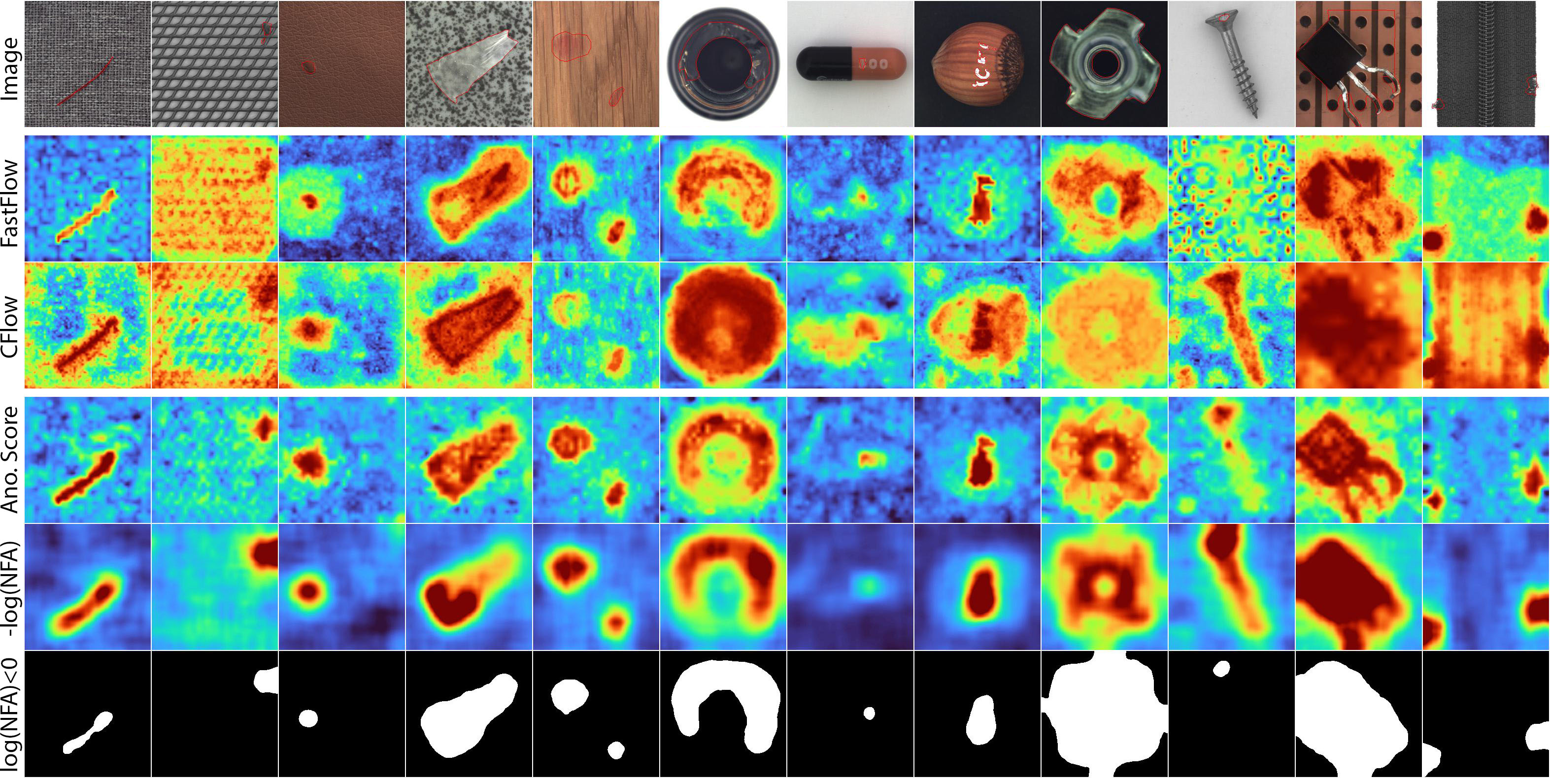
Figure 5: Example results for several categories, compared with FastFlow and CFlow in the second and third rows. The Last three rows correspond to our method: the anomaly score defined in (1), the NFA-based anomaly score ($-\log\textit{NFA}$), and the segmentation obtained with the automatic threshold $\log\textit{NFA}<0$. While other methods achieve a very good performance, in some cases they present artifacts and over-estimated anomaly scores. Our anomaly score achieves very good visual and numerical results, spotting anomalies with high confidence, and the NFA-based anomaly score is softer and cleaner. Finally, the segmentation with the automatic threshold on the NFA is also able to spot and segment the anomaly accurately.

Finally, Figure 5 presents typical example results of anomalous images from various categories, and their comparison with other methods, for visual evaluation, and in Figure 6 some example of normal images, in order to check that the anomaly maps present low values, and no detection is made.

4.2 Results on other datasets

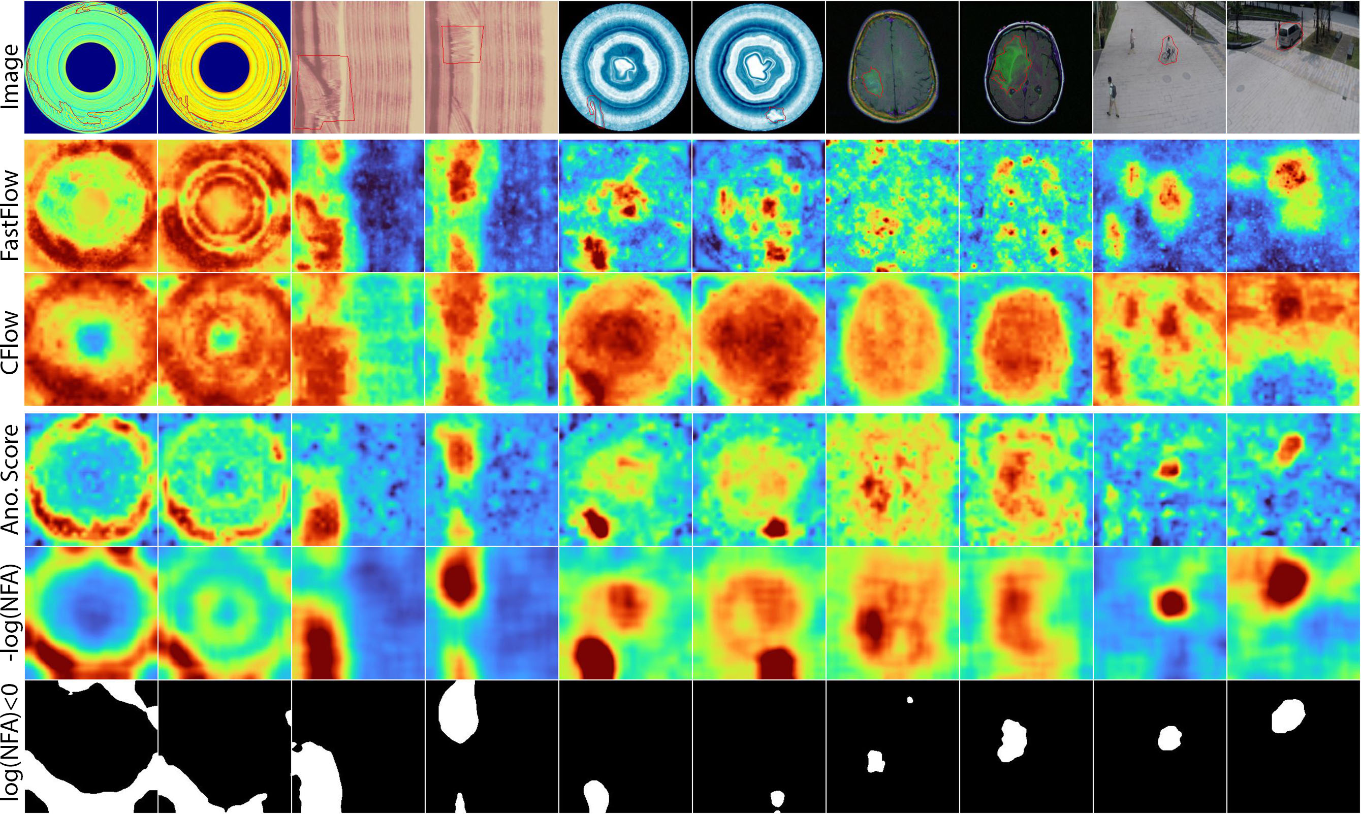
Figure 7: Examples of typical results on BeanTech, LGG MRI, and STC datasets. The first row shows the original images with super-imposed ground truth. The second and third rows show the results of FastFlow and CFlow for comparison. The Last three rows are different outputs of our method: the anomaly score defined in (1), the NFA-based anomaly score ($-\log\textit{NFA}$), and the anomaly segmentation with $\log\textit{NFA}<0$. Again, our anomaly score achieves very good visual and numerical results, and is able to detect the anomalies with great confidence.

In this section, we present the results obtained on the other datasets: BeanTeach (BT), LGG MRI (MRI) and ShanghaiTech Campus (STC). Although our work is motivated by the industrial inspection task, we also evaluate the performance on other datasets that are very different from that scenario. The results reported here demonstrate the robustness and generalization capability of the proposed approach (c.f. Table 5). For all datasets we obtained excellent results, reaching top performance for almost all metrics and datasets. The comparison considers the best-performing methods on MVTec, and also the ones that also use NFs. For a fair comparison, all results were obtained by training the other methods with different hyperparameters to achieve the best possible results. In the case some combination of metric-dataset were reported in the original papers, we corroborated that we were obtaining the same results. Typical qualitative results are shown in Figure 7.

	Method\DS	BT01	BT02	BT03	BT AV.	MRI	STC
AUROC	FastFlow	95.98	96.69	99.32	97.33	82.51	95.51
	CFlow	94.29	96.13	99.58	96.67	86.41	96.90
	U-Flow	97.70	96.93	99.76	98.13	93.55	87.19
AUPRO	FastFlow	76.23	62.39	96.60	78.41	47.48	73.67
	CFlow	60.19	54.72	98.32	71.08	59.47	82.05
	U-Flow	80.06	66.49	98.83	81.79	71.74	47.54
IoU	FFlow (O)	0.446	0.481	0.751	0.559	0.217	0.737
	FFlow (F)	0.366	0.479	0.583	0.476	0.010	0.235
	CFlow (O)	0.464	0.448	0.924	0.612	0.218	0.462
	CFlow (F)	0.458	0.414	0.774	0.549	0.209	0.462
	U-Flow	0.488	0.288	0.936	0.571	0.219	0.462
IMAGE	FastFlow	100.0	89.13	96.65	95.26	61.49	74.04
	CFlow	94.95	79.68	99.96	91.53	42.56	66.39
	U-Flow	99.42	88.72	99.72	95.95	72.60	64.59

Table 5: Results on BeanTeach (BT) [24], LGG MRI (MRI) [3] and ShanghaiTech Campus (STC) [22] datasets. Comparison with FastFlow [42] and CFlow [14]. For almost all metrics and datasets, our method obtains the best results, outperforming the other methods. “Image” metric refers to image-level AUROC.

4.3 Implementation and complexity details

The method was implemented in PyTorch [25], using PyTorch Lightning [10]. The NFs were implemented using the FrEIA Framework [1], and for all tested feature extractors we used PyTorch Image Models [38]. In all cases, training was performed in a GeForce RTX 2080 Ti.

For the MS-CaIT, the input sizes are 448 and 224 pixels in width and height. The Normalizing Flow has 2 flow stages with 4 flow steps each. For computing the NFA, we used $p=0.9$, $w_{1}=5$, and $w_{2}=3$. Note that $p$, $w_{1}$, and $w_{2}$ are not decision thresholds, but design parameters that were chosen taking into account the size of the anomalies, and were always kept the same for all experiments.

Our method only uses four flow steps in each scale. As a result, it has fewer trainable parameters than FastFlow and CFlow, as shown in Table 6.

5 Ablation Study

In this section, we study and provide unbiased assessments regarding some of the contributions of this work: the significance of the U-shaped architecture and the benefits of the multi-scale Transformer feature extractor MS-CaiT. Both results are shown all together in Table 7, and explained in the following sections.

Also, to get some insights and visualize the distinction between normal and abnormal samples, we include Figure 4, which displays the distribution of the NFA-based anomaly score ($-\log\textit{NFA}$) for both normal and anomalous pixels. The solid vertical line represents the automatic threshold ($\log\text{NFA}=0$), and a dashed line the oracle-like threshold, i.e. the best possible threshold for IoU on the test set. The distributions are clearly separated, and the automatic threshold is located very close to the optimal point, supporting the a contrario thresholding strategy.

5.1 Ablation: U-shape

One of the contributions of the presented work is to propose a multi-level integration mechanism, by introducing the well-known U-shape architecture design to the Normalizing Flow’s framework. In order to demonstrate that this architecture better integrates the information of the different scales, we compare the results obtained in terms of AUROC against a modification of the architecture, in which each flow stage runs in parallel, and the per-scale anomaly maps are merged at the end by just averaging them, as done by other methods such as FastFlow [42]. Additionally, we compare the results obtained using each scale separately. The results, presented in the top half of Table 7, show that the U-merging strategy improves the performance in almost all cases. Furthermore, this strategy where the output of one scale inputs the next one, allows to use less flow steps for each scale, resulting in a network with fewer parameters, as shown in Section 4.3.

5.2 Ablation: feature extraction with MS-CaiT

Feature Extractor	FastFlow	CFlow	Ours
ResNet18	4.9 M	5.5 M	4.3 M
WideResnet50-2	41.3 M	81.6 M	34.8 M
CaIT M48	14.8 M	10.5 M	8.9 M
MS-CaiT	-	-	12.2 M

Table 6: Complexity analysis: comparison of number of trainable parameters for different feature extractors.

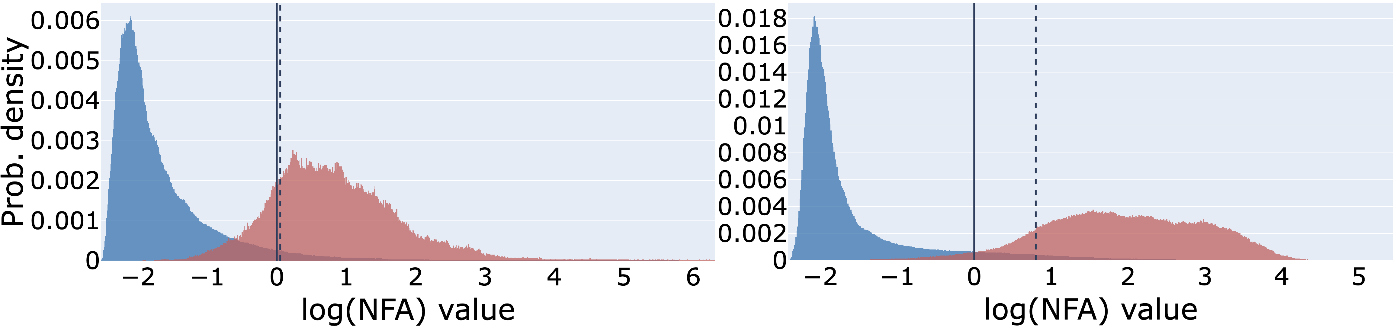
Figure 4: NFA-based anomaly score ($-\log\text{NFA}$) distribution for the bottle (left) and metal nut (right) classes. Blue corresponds to normal pixels, and red to anomalous. The vertical line stands for $\log\text{NFA}=0$, which corresponds nearly to the optimal point. Plots for other classes are included in the Appendix.

	Carp.	Grid	Leat.	Tile	Wood	Bott.	Cable	Caps.	HNut	MNut	Pill	Screw	Toot.	Tran.	Zipp.	Total
Scale 1	99.08	97.40	99.32	94.97	93.45	98.33	98.11	98.87	99.09	97.89	98.67	99.44	98.74	96.46	98.55	97.89
Scale 2	99.12	97.09	99.42	96.47	96.26	97.23	97.60	98.07	98.63	97.86	98.62	99.18	97.86	97.21	97.29	97.86
Average	99.44	98.25	99.52	97.27	96.40	98.61	98.50	98.85	99.16	98.29	99.12	99.50	98.78	97.66	98.69	98.54
Ours	99.42	98.49	99.59	97.54	97.49	98.65	98.61	99.02	99.30	98.82	99.35	99.49	98.79	97.87	98.60	98.74
ResNet	98.80	98.26	99.37	94.53	94.50	98.00	96.96	98.46	98.63	96.70	97.45	98.01	98.20	98.38	97.43	97.58
Arch.	wide	r18	r18	wide	r18	r18	wide	wide	wide	wide	wide	wide	r18	wide	wide	-
F. steps	6	6	4	8	6	4	4	4	4	4	4	6	6	4	4	-
MViT2	98.74	97.73	99.20	93.83	94.75	92.79	96.98	98.83	97.50	96.39	97.36	97.69	87.14	97.00	96.39	96.15

Table 7: Ablation results. The middle row (in-between horizontal lines), which shows the pixel-level ROC-AUC results of our proposed method (U-Flow), serves for comparison for the top and bottom halves of the table. Top half: ablation study for the scale-merging strategy. Results using the anomaly scores generated by each scale independently, and a naive way of merging them (average). Bottom half: ablation study for the feature extractor. The proposed method (that uses MS-CaIT) is compared with ResNet and MViT2 feature extractors. Each category shows the AUROC of the best variant we could obtain, varying several hyper-parameters, such as the architecture (wide-resnet-50 or resnet-18) and the number of flow steps.

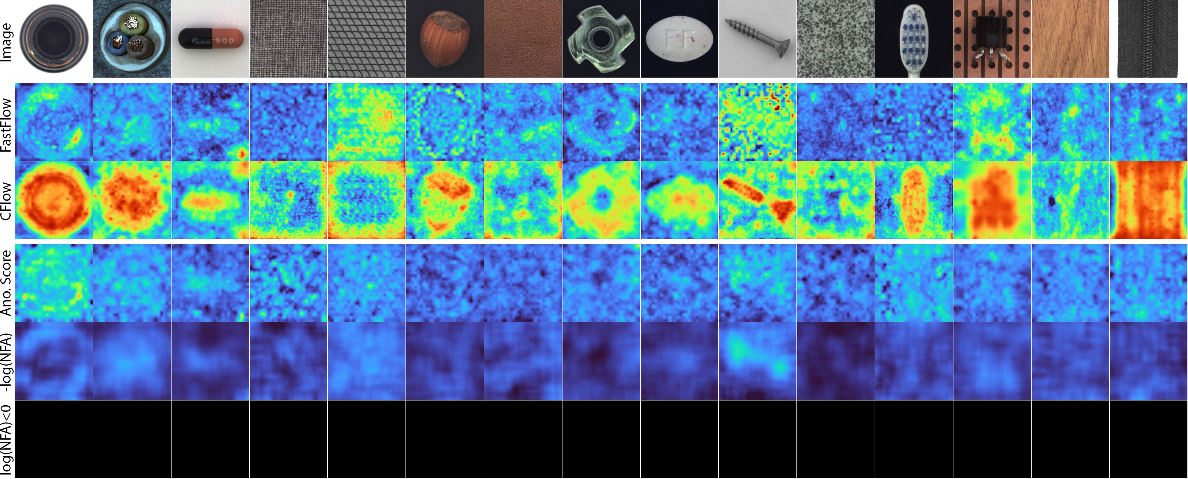
Figure 6: Normal images examples.

From the upper half of Table 7, it is also clear that utilizing image Transformers at various scales in MS-CaiT significantly improves the results, even if each of them provides already a multi-scale representation. Note that both scale-merging strategies outperform the results obtained by each individual Transformer.

In addition, in this section, we compare the results obtained by the proposed MS-CaIT feature extractor, with the most common ResNet variants used in the literature: ResNet-18 and Wide-ResNet-50, and the multi-scale Transformer MViT2. Table 7’s bottom half makes it clear that the MS-CaiT feature extractor performs far better than ResNet variants and MViT2. Note that, in favor of the ResNet extractors, for each category, we picked the best result obtained by both variants, and also varied several hyper-parameters, for example, the amount of flow steps in each scale, while for MS-CaIT we use always the same exact architecture.

6 Conclusion

In this work, we introduced a novel anomaly detection method that achieves state-of-the-art results on various datasets and even outperforms them in most cases. By making use of modern techniques with outstanding performance, such as Transformers and Normalizing Flows, we developed a method that exploits their characteristics to integrate them with classic statistical modeling. Our approach consists of three phases that follow one another, and we presented a clear and compelling contribution for each one: (i) We propose a new feature extractor using pre-trained Transformers, to build a multi-scale representation. (ii) We integrate the U-shape architecture into the Normalizing Flow framework, creating a complete invertible architecture that settles the theoretical foundations for the NFA computation, by ensuring independence in the embedding not only intra-scale but also inter-scales. And (iii) we derive an unsupervised threshold based on the a contrario framework, that exploits the U-Flow embeddings to produce excellent anomaly segmentation results.

Appendix

We present here a further analysis of the proposed method and more experimental results including failure cases and limitations.

Appendix A Analysis of the Normalizing Flow embedding

To complement the results included in the main submission, in this section we propose to analyze visually the embeddings produced by the NF, by mapping them to a three-dimensional space using the T-distributed Stochastic Neighbor Embedding (T-SNE) algorithm. Results for various categories are shown in Figure 8. Each dot in this 3D space represents a different test image, and they are colored according to the type of defect. Green dots are always normal samples (i.e. anomaly-free images).

For generating this mapping, we could apply T-SNE directly to the entire volume $z$. But instead, aiming to reduce the input dimensionality, we apply an intermediate step. Recalling that for each scale $l$ we have an embedding $z_{l}$ of size $[C_{l},H_{l},W_{l}]$, we keep for each $k=\{1,\dots,C_{l}\}$ the mean and standard deviation of the squared values of the volume, constructing a feature vector of dimension $2*C_{l}$ for each image. The final feature vector, concatenating vectors from all scales, has size $2\sum_{l}C_{l}$. These feature vectors are used as input for the T-SNE algorithm.

It is easy to observe that, both normal samples and defects types, reveal a clustering structure. Even though the method was aimed at separating abnormal samples from normal samples (green dots), it is interesting to note that this representation evidences that there is also a good separation between different types of defects, giving a hint that this technique could be also potentially applied for defects classification.

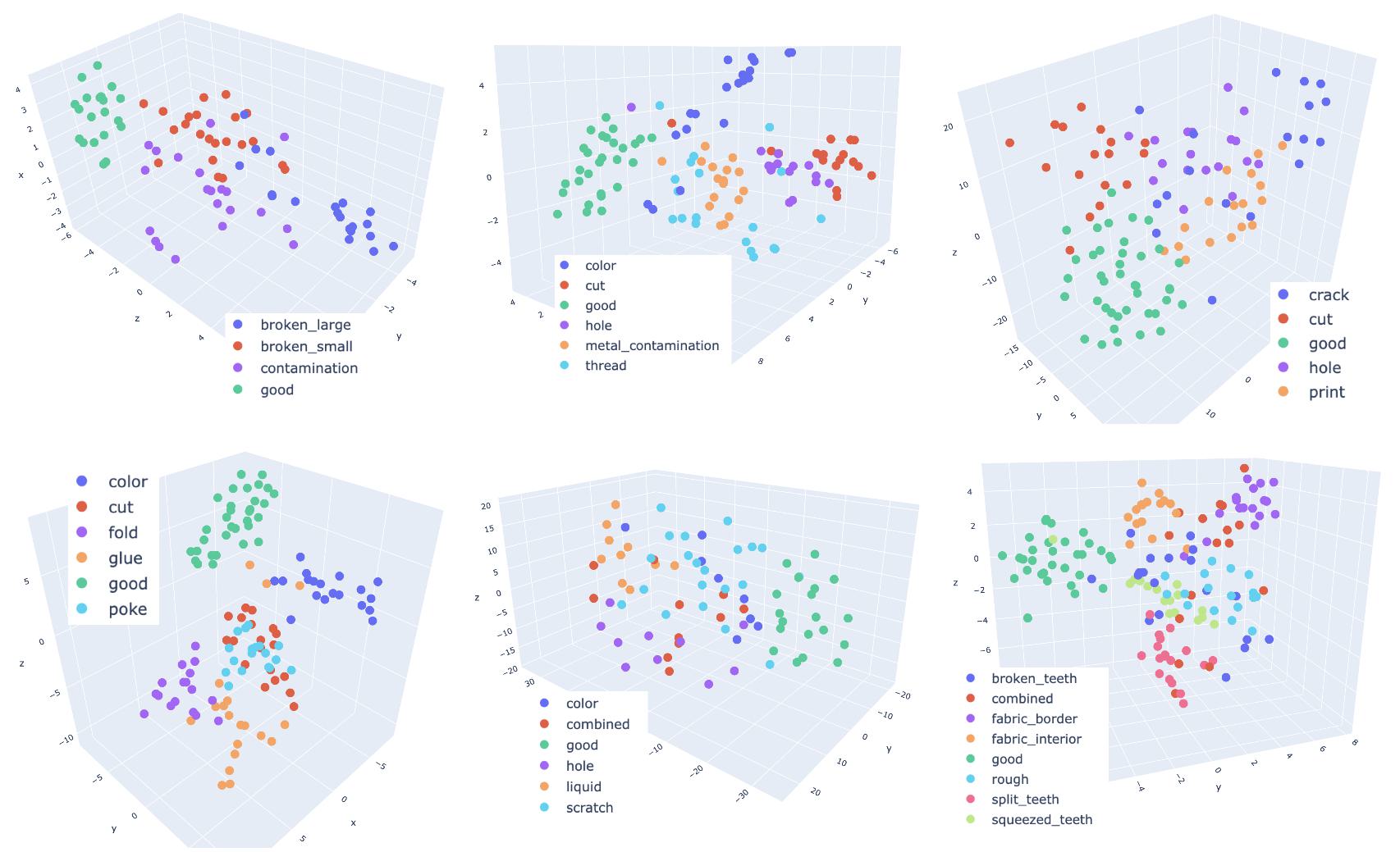
Figure 8: T-SNE embeddings. Top row: bottle, carpet and hazelnut. Bottom row: leather, wood and zipper. Normal samples are always in green, and other colors correspond to different defect types. It can be seen a very good separation not only for the normal samples, but also for each different type of defect.

Appendix B Analysis of the proposed multiple hypothesis testing procedure

To extend the analysis shown in Figure 4, we present Figure 9 with the distributions of normal and anomalous pixels for all categories. Both distributions are the normalized histograms (such that the integral equals one), of the $-\log(\text{NFA})$ values for all pixels. For all categories we obtain a good separation between normal and anomalous pixels. Also, the natural threshold $\log(\text{NFA})=0$, indicated with a solid vertical line, usually lays near the optimal point, and also close to the vertical dashed line, which indicates the best possible threshold in terms of segmentation IoU (the oracle-like threshold). Actually this is not surprising, as the NF is supposed to produce a closed form representation (a white Gaussian process) of the transformed density, which enables to derive automatic thresholds without requiring to “manually” learn them. The fact that these thresholds are close is a confirmation that the theoretical densities are close to the sample densities.

The NFA computation explained in Section 3.3.2 is based on the detection of concentrations of pixels with suspiciously high values. It follows a very simple aggregation technique, where the NFA value for each pixel $(i,j)$ depends on its neighborhood, that is defined as a square window centered on itself. Although very simple, this technique helps to obtain an anomaly measure that is robust to outliers and achieves excellent results. However, it also suffers from some drawbacks which are exclusively related to the definition of the tested regions (and could be further improved and mitigated), as explained in the following subsection.

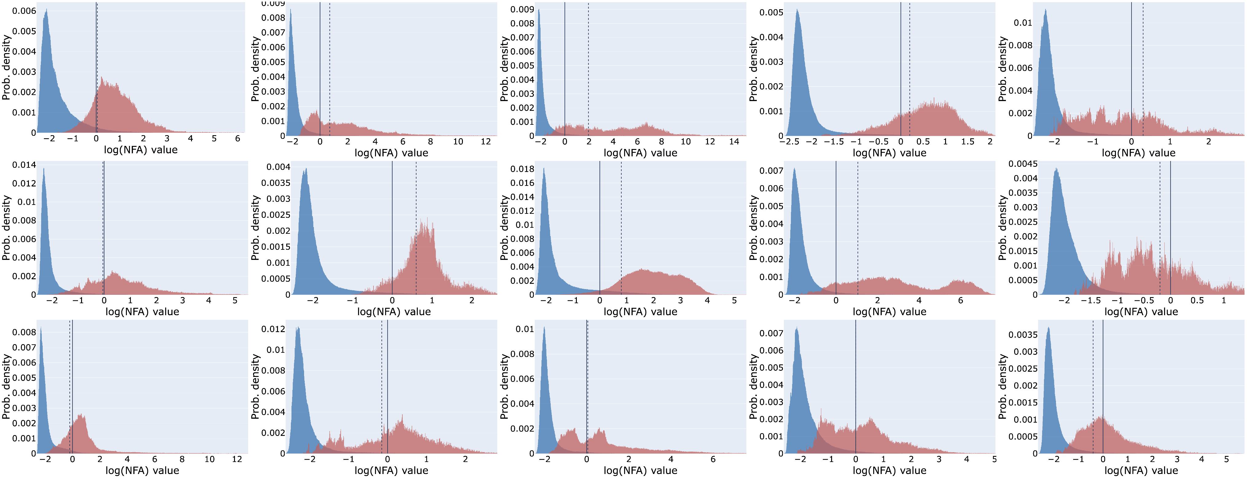
Figure 9: NFA-based anomaly score ($-\log\text{NFA}$) distribution of normal pixels (blue) and anomalous pixels (red) for all categories in alphabetical order. Top row: bottle, cable, capsule, carpet and grid. Middle row: hazelnut, leather, metal nut, pill, and screw. Bottom row: tile, toothbrush, transistor, wood, and zipper. The vertical solid line represents the automatic threshold $\log\text{NFA}=0$ and the dashed line the oracle-like threshold. This figure corresponds to Figure 4.

B.1 Failure cases

This aggregation technique based on the neighborhood of each pixel, makes the NFA-based anomaly maps smoother, and leads to two undesired collateral effects in the segmentation maps:

• For small defects: in some cases where the anomaly is subtle and small, the square window considered around each pixel could have a smoothing effect, that also lowers the anomaly score, even to the point that it is not detected with the automatic threshold. This cases are shown in the two leftmost columns in Figure 10 (cable and capsule).

• For defects that are very thin, but show a high anomaly score: the effect is sometimes to obtain a too coarse segmentation, as shown in the two rightmost columns of Figure 10 (grid and tile).

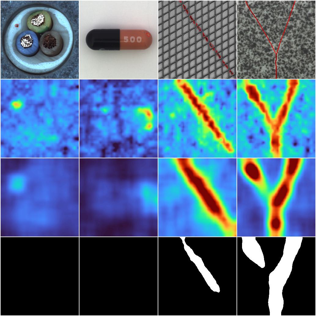
Figure 10: Example of failure cases in anomaly segmentation maps. First row: original images with superimposed ground truths. Second row: likelihood-based anomaly score. Third and fourth rows: NFA-based anomaly score, and segmentation mask obtained with the natural threshold $\log\text{NFA}=0$. The first two examples (cable and capsule) show some defects that are clearly detected with the likelihood-based anomaly score, but the NFA aggregation strategy makes the NFA-based anomaly score to be too smoothed and the defects are not being caught using the natural threshold. The last two examples (grid and tile) show defects that although being detected, present a coarse segmentation.

Note that this drawbacks apply exclusively to the NFA-based anomaly score. The likelihood-based anomaly score always exhibits accurate results. It is possible to improve anomaly segmentation, and to certainly obtain higher IoU, if instead of considering rectangular regions in the embedding volumes, we consider a larger set of tests enabling a richer variety of shapes and sizes that better adjust the support of the anomalies. Such sets of tests have already been proposed and explored in [35, 32].

Appendix C More example results

C.1 Anomalous images

In this section we present a larger set of experimental results. We display two images for each category, with different types of defects. Texture examples are shown in Figure 11, and object examples are shown in Figures 12 and 13.

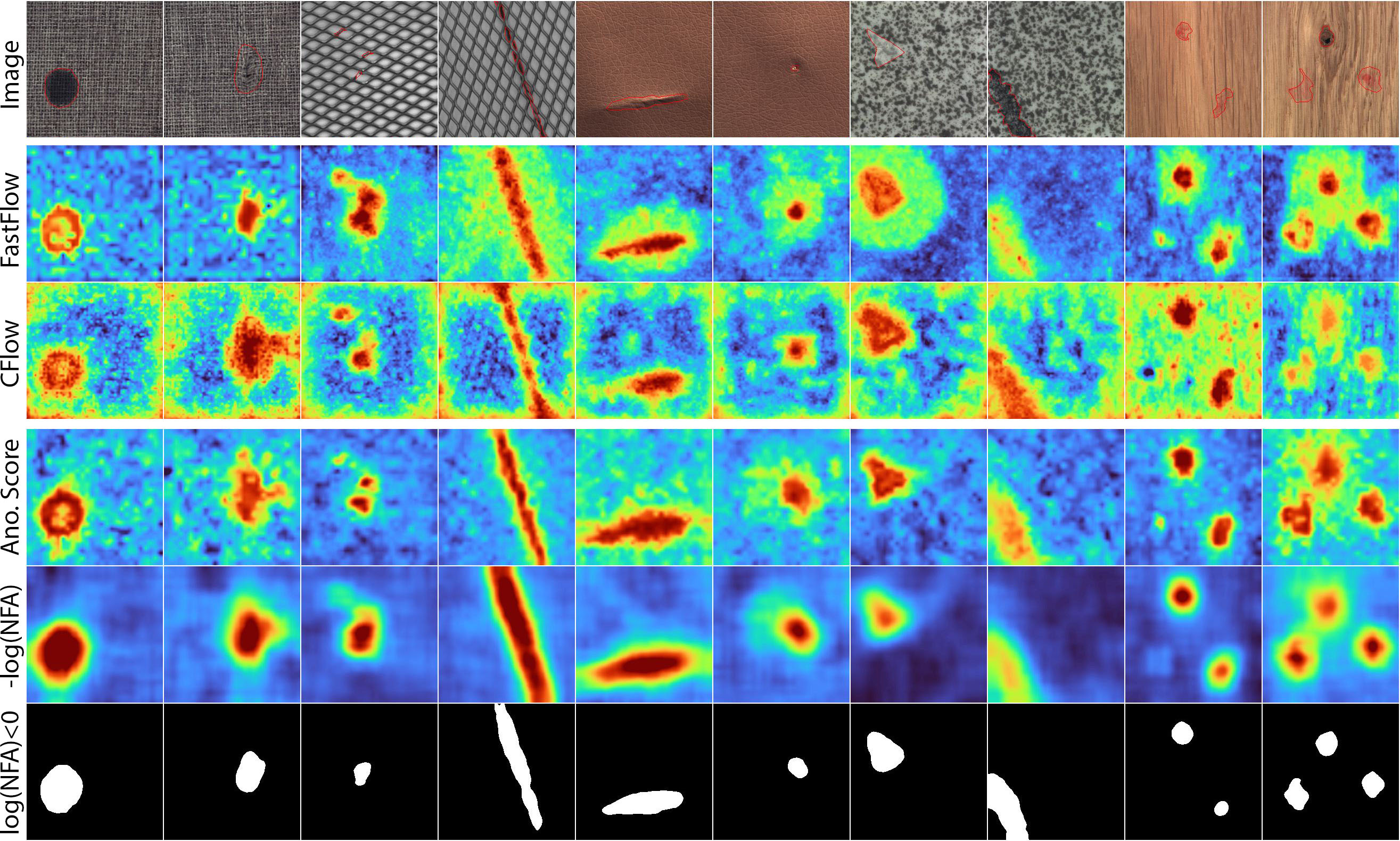
Figure 11: Textures: carpet, grid, leather, tile and wood.

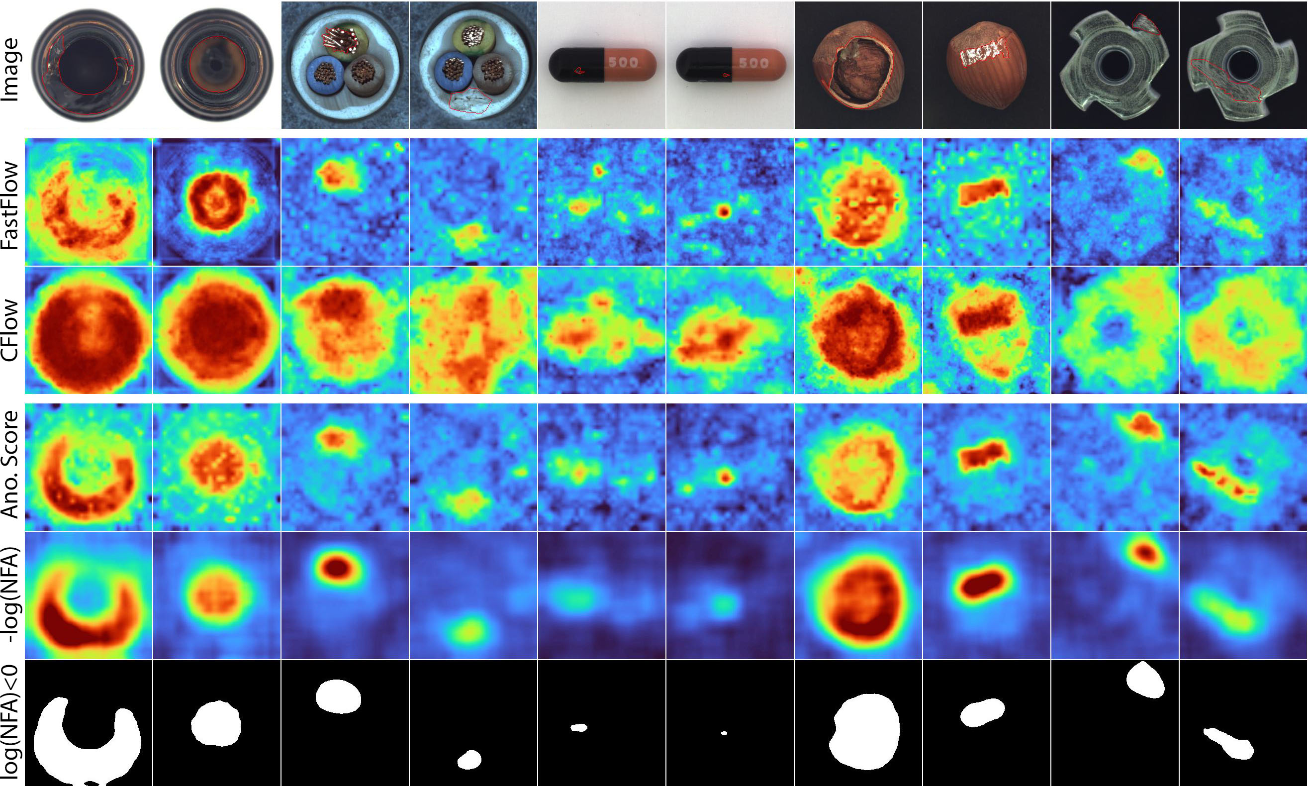
Figure 12: Objects 1: bottle, cable, capsule, hazelnut and metal nut.

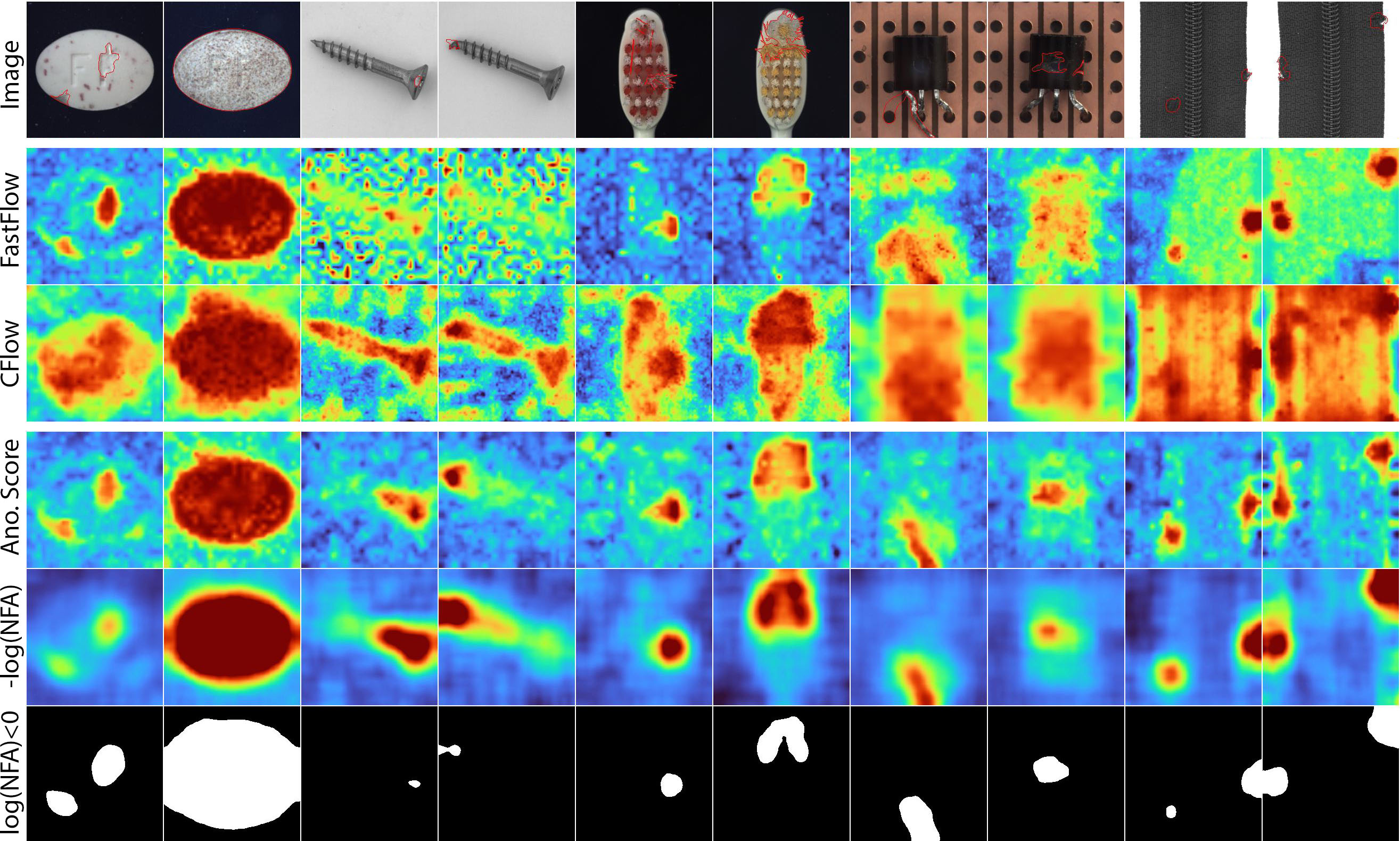
Figure 13: Objects 2: pill, screw, toothbrush, transistor and zipper.

C.2 Normal images

Also, it is interesting to check how the anomaly scores behave with anomaly-free images. As shown in Figure 6, in this section we add more normal examples, corresponding to the other datasets: BeanTech, LGG MRI, and STC, in Figure 14. As can be seen, the anomaly scores are always low, and we do not detect any anomalous pixel in the segmentations.

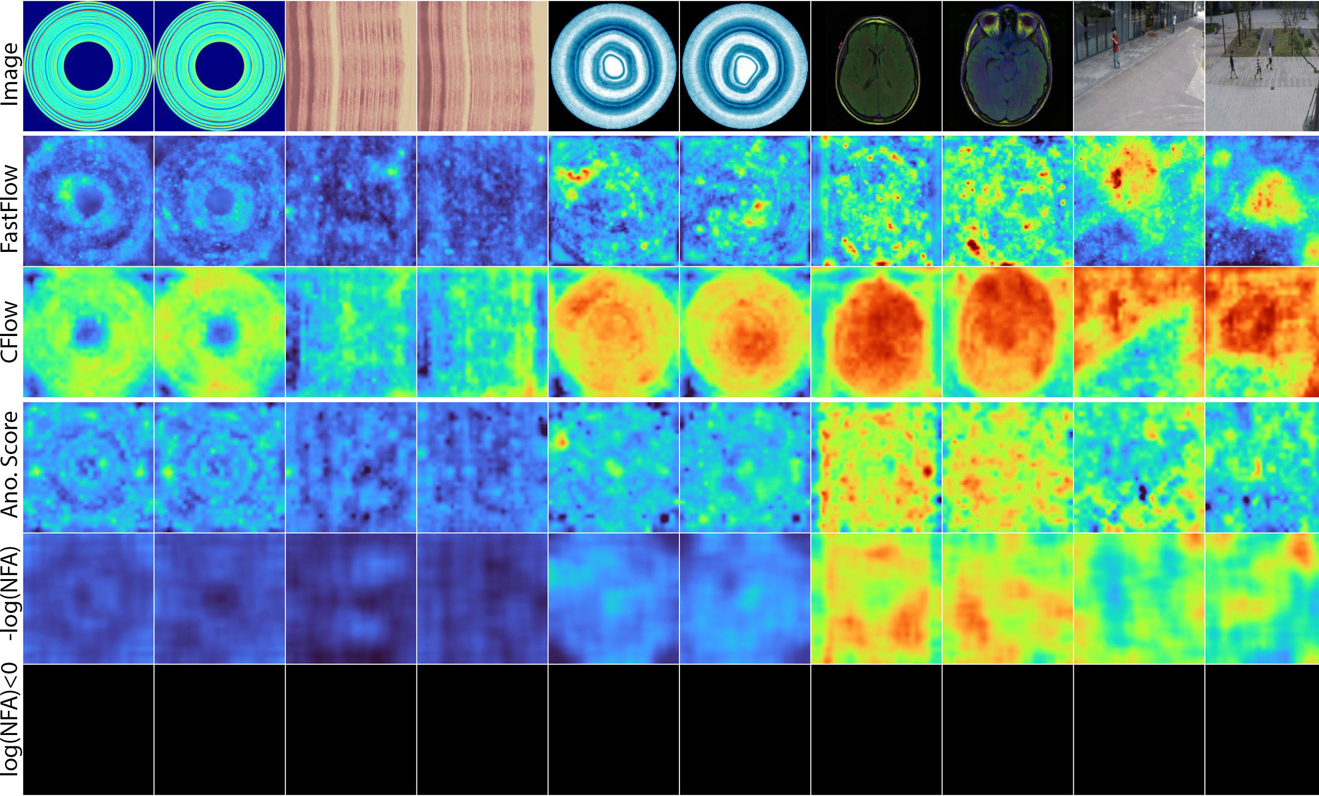
Figure 14: Normal images examples of BeanTech, LGG MRI, and STC.

C.3 Unexpected surprises: detection of actual unlabeled anomalies in images

While visually inspecting the results, we found some cases where unlabeled anomalies were detected. A careful look reveals that these structures are actually different kinds of anomalies, and therefore it is actually correct to detect them. This kind of “false true detections” unfairly penalize the method’s performance.

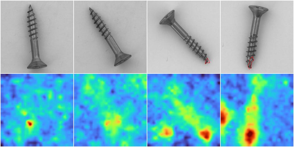
(a) Example of a subtle fluff in the background for the screw category.

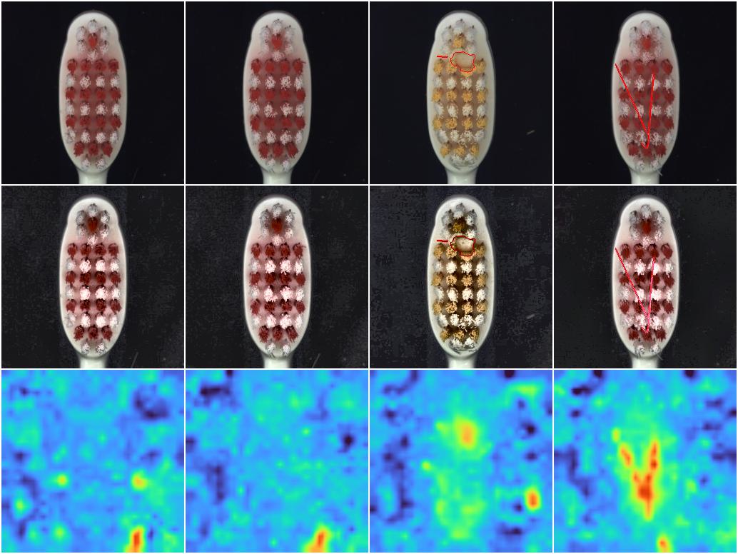
(b) Examples for toothbrush. Some defect in the background is being detected.

Figure 15: Examples of “false true” anomalies. Our method detects some anomalies that are not supposed to be there, and that are not labelled. For better visualization we recommend to zoom-in.

Two such examples are shown in Figure 15. Figure 15(a) displays four images of the screw category, in which we can observe a subtle fluff in the background, almost unnoticeable to the naked eye, that correctly stands out in the anomaly score map. The two leftmost images correspond to images labeled as anomaly-free samples, while the two rightmost ones present labeled defects somewhere else, that are also correctly detected. Similarly, Figure 15(b) shows four images of the toothbrush category, that also present some defects in the background. As they are very difficult to see with the naked eye, we included a contrast-enhanced version of the image in the middle row for visualization purposes. Again, these defects are correctly detected but they were not supposed to be there, and since they are not labeled they penalize the results when computing the evaluation metrics.

Appendix D Implementation details

• Image upsampling. To compute the anomaly scores, we use the embeddings $z_{ijk}^{l}$ for each scale $l$ and then merge them. As for each scale $l$ the spatial size of the embedding $(H_{l},W_{l})$ is different, the low resolution embeddings have to be upsampled to match the size of the (original) finer resolution one. This operation was not specified in Section 3.3, only for the sake of simplicity, as it does not affect or adds any other consideration, as the only operation that is performed following this upsampling is merging the scales, that are ensured to be independent thanks to the Normalizing Flow architecture.

• Training. The training is executed using always the same architecture parameters. The only hyperparameters that are different between categories are related only to the optimization itself: the learning rate varies between $3\times 10^{-3}$ and $3\times 10^{-5}$, and the batch size, that varies between 10 and 30, depending on the category.

• NFA precision. The computation of the NFA-based anomaly score relies on the Binomial tail, which integrates extremely small values. To do so, it could be very important to work with high precision. The results reported are obtained with high precision computation. However, the difference in the metric with standard precision is really low, and the computation is much faster. Therefore, although getting slightly lower results, it is recommended to use standard precision. In any case, the code allows the user to easily choose between the two options, using a command line argument.

References

- [1] Lynton Ardizzone, Till Bungert, Felix Draxler, Ullrich Köthe, Jakob Kruse, Robert Schmier, and Peter Sorrenson. Framework for Easily Invertible Architectures (FrEIA), 2018-2022.
- [2] Paul Bergmann, Michael Fauser, David Sattlegger, and Carsten Steger. Mvtec ad–a comprehensive real-world dataset for unsupervised anomaly detection. In Proceedings of the IEEE/CVF conference on computer vision and pattern recognition, pages 9592–9600, 2019.
- [3] Mateusz Buda, Ashirbani Saha, and Maciej A Mazurowski. Association of genomic subtypes of lower-grade gliomas with shape features automatically extracted by a deep learning algorithm. Computers in biology and medicine, 109:218–225, 2019.
- [4] Niv Cohen and Yedid Hoshen. Sub-image anomaly detection with deep pyramid correspondences. arXiv preprint arXiv:2005.02357, 2020.
- [5] Thomas Defard, Aleksandr Setkov, Angelique Loesch, and Romaric Audigier. Padim: a patch distribution modeling framework for anomaly detection and localization. In International Conference on Pattern Recognition, pages 475–489. Springer, 2021.
- [6] Agnes Desolneux, Lionel Moisan, and Jean-Michel Morel. From gestalt theory to image analysis: a probabilistic approach, volume 34. Springer Science & Business Media, 2007.
- [7] Laurent Dinh, David Krueger, and Yoshua Bengio. Nice: Non-linear independent components estimation. arXiv preprint arXiv:1410.8516, 2014.
- [8] Laurent Dinh, Jascha Sohl-Dickstein, and Samy Bengio. Density estimation using real nvp. arXiv preprint arXiv:1605.08803, 2016.
- [9] Alexey Dosovitskiy, Lucas Beyer, Alexander Kolesnikov, Dirk Weissenborn, Xiaohua Zhai, Thomas Unterthiner, Mostafa Dehghani, Matthias Minderer, Georg Heigold, Sylvain Gelly, et al. An image is worth 16x16 words: Transformers for image recognition at scale. arXiv preprint arXiv:2010.11929, 2020.
- [10] William Falcon and The PyTorch Lightning team. PyTorch Lightning, 3 2019.
- [11] Haoqi Fan, Bo Xiong, Karttikeya Mangalam, Yanghao Li, Zhicheng Yan, Jitendra Malik, and Christoph Feichtenhofer. Multiscale vision transformers. In Proceedings of the IEEE/CVF International Conference on Computer Vision, pages 6824–6835, 2021.
- [12] Marina Gardella, Pablo Musé, Jean-Michel Morel, and Miguel Colom. Noisesniffer: a fully automatic image forgery detector based on noise analysis. In 2021 IEEE International Workshop on Biometrics and Forensics (IWBF), pages 1–6. IEEE, 2021.
- [13] Ian Goodfellow, Jean Pouget-Abadie, Mehdi Mirza, Bing Xu, David Warde-Farley, Sherjil Ozair, Aaron Courville, and Yoshua Bengio. Generative adversarial nets. In Advances in Neural Information Processing Systems, pages 2672–2680, 2014.
- [14] Denis Gudovskiy, Shun Ishizaka, and Kazuki Kozuka. Cflow-ad: Real-time unsupervised anomaly detection with localization via conditional normalizing flows. In Proceedings of the IEEE/CVF Winter Conference on Applications of Computer Vision, pages 98–107, 2022.
- [15] Kaiming He, Xiangyu Zhang, Shaoqing Ren, and Jian Sun. Deep residual learning for image recognition. In Proceedings of the IEEE conference on computer vision and pattern recognition, pages 770–778, 2016.
- [16] Jörn-Henrik Jacobsen, Arnold Smeulders, and Edouard Oyallon. i-revnet: Deep invertible networks. arXiv preprint arXiv:1802.07088, 2018.
- [17] Durk P Kingma and Prafulla Dhariwal. Glow: Generative flow with invertible 1x1 convolutions. Advances in neural information processing systems, 31, 2018.
- [18] Diederik P. Kingma and Max Welling. Auto-encoding variational bayes. In 2nd International Conference on Learning Representations, 2014.
- [19] Sungwook Lee, Seunghyun Lee, and Byung Cheol Song. Cfa: Coupled-hypersphere-based feature adaptation for target-oriented anomaly localization. arXiv preprint arXiv:2206.04325, 2022.
- [20] Chun-Liang Li, Kihyuk Sohn, Jinsung Yoon, and Tomas Pfister. Cutpaste: Self-supervised learning for anomaly detection and localization. In Proceedings of the IEEE/CVF Conference on Computer Vision and Pattern Recognition, pages 9664–9674, 2021.
- [21] Yanghao Li, Chao-Yuan Wu, Haoqi Fan, Karttikeya Mangalam, Bo Xiong, Jitendra Malik, and Christoph Feichtenhofer. Improved multiscale vision transformers for classification and detection. arXiv preprint arXiv:2112.01526, 2021.
- [22] W. Liu, D. Lian W. Luo, and S. Gao. Future frame prediction for anomaly detection – a new baseline. In 2018 IEEE Conference on Computer Vision and Pattern Recognition (CVPR), 2018.
- [23] David G. Lowe. Perceptual Organization and Visual Recognition. Kluwer Academic Publishers, USA, 1985.
- [24] Pankaj Mishra, Riccardo Verk, Daniele Fornasier, Claudio Piciarelli, and Gian Luca Foresti. Vt-adl: A vision transformer network for image anomaly detection and localization. In 2021 IEEE 30th International Symposium on Industrial Electronics (ISIE), pages 01–06. IEEE, 2021.
- [25] Adam Paszke, Sam Gross, Francisco Massa, Adam Lerer, James Bradbury, Gregory Chanan, Trevor Killeen, Zeming Lin, Natalia Gimelshein, Luca Antiga, Alban Desmaison, Andreas Kopf, Edward Yang, Zachary DeVito, Martin Raison, Alykhan Tejani, Sasank Chilamkurthy, Benoit Steiner, Lu Fang, Junjie Bai, and Soumith Chintala. Pytorch: An imperative style, high-performance deep learning library. In Advances in Neural Information Processing Systems 32, pages 8024–8035. Curran Associates, Inc., 2019.
- [26] Olaf Ronneberger, Philipp Fischer, and Thomas Brox. U-net: Convolutional networks for biomedical image segmentation. In International Conference on Medical image computing and computer-assisted intervention, pages 234–241. Springer, 2015.
- [27] Karsten Roth, Latha Pemula, Joaquin Zepeda, Bernhard Schölkopf, Thomas Brox, and Peter Gehler. Towards total recall in industrial anomaly detection. In Proceedings of the IEEE/CVF Conference on Computer Vision and Pattern Recognition, pages 14318–14328, 2022.
- [28] Marco Rudolph, Bastian Wandt, and Bodo Rosenhahn. Same same but differnet: Semi-supervised defect detection with normalizing flows. In Proceedings of the IEEE/CVF winter conference on applications of computer vision, pages 1907–1916, 2021.
- [29] Olga Russakovsky, Jia Deng, Hao Su, Jonathan Krause, Sanjeev Satheesh, Sean Ma, Zhiheng Huang, Andrej Karpathy, Aditya Khosla, Michael Bernstein, Alexander C. Berg, and Li Fei-Fei. ImageNet Large Scale Visual Recognition Challenge. International Journal of Computer Vision (IJCV), 115(3):211–252, 2015.
- [30] Thomas Schlegl, Philipp Seeböck, Sebastian M Waldstein, Ursula Schmidt-Erfurth, and Georg Langs. Unsupervised anomaly detection with generative adversarial networks to guide marker discovery. In Intl. Conf. on Information Processing in Medical Imaging, pages 146–157. Springer, 2017.
- [31] Karen Simonyan and Andrew Zisserman. Very deep convolutional networks for large-scale image recognition. arXiv preprint arXiv:1409.1556, 2014.
- [32] Matías Tailanian, Pablo Musé, and Álvaro Pardo. A contrario multi-scale anomaly detection method for industrial quality inspection. arXiv preprint arXiv:2205.11611, 2022.
- [33] Hugo Touvron, Matthieu Cord, Alexandre Sablayrolles, Gabriel Synnaeve, and Hervé Jégou. Going deeper with image transformers. In Proceedings of the IEEE/CVF International Conference on Computer Vision, pages 32–42, 2021.
- [34] Chin-Chia Tsai, Tsung-Hsuan Wu, and Shang-Hong Lai. Multi-scale patch-based representation learning for image anomaly detection and segmentation. In Proceedings of the IEEE/CVF Winter Conference on Applications of Computer Vision, pages 3992–4000, 2022.
- [35] Rafael Grompone von Gioi, Charles Hessel, Tristan Dagobert, Jean-Michel Morel, and Carlo de Franchis. Ground visibility in satellite optical time series based on a contrario local image matching. Image Processing On Line, 11:212–233, 2021.
- [36] Rafael Grompone Von Gioi, Jérémie Jakubowicz, Jean-Michel Morel, and Gregory Randall. On straight line segment detection. Journal of Mathematical Imaging and Vision, 32(3):313–347, 2008.
- [37] Qian Wan, Yunkang Cao, Liang Gao, Weiming Shen, and Xinyu Li. Position encoding enhanced feature mapping for image anomaly detection. In 2022 IEEE 18th International Conference on Automation Science and Engineering (CASE), pages 876–881. IEEE, 2022.
- [38] Ross Wightman. Pytorch image models. https://github.com/rwightman/pytorch-image-models, 2019.
- [39] Shinji Yamada, Satoshi Kamiya, and Kazuhiro Hotta. Reconstructed student-teacher and discriminative networks for anomaly detection. arXiv preprint arXiv:2210.07548, 2022.
- [40] Jie Yang, Yong Shi, and Zhiquan Qi. Dfr: Deep feature reconstruction for unsupervised anomaly segmentation. arXiv preprint arXiv:2012.07122, 2020.
- [41] Jihun Yi and Sungroh Yoon. Patch svdd: Patch-level svdd for anomaly detection and segmentation. In Proceedings of the Asian Conference on Computer Vision, 2020.
- [42] Jiawei Yu, Ye Zheng, Xiang Wang, Wei Li, Yushuang Wu, Rui Zhao, and Liwei Wu. Fastflow: Unsupervised anomaly detection and localization via 2d normalizing flows. arXiv preprint arXiv:2111.07677, 2021.