Diffusion Model Based Posterior Sampling for
Noisy Linear Inverse Problems

Abstract

We consider the ubiquitous linear inverse problems with additive Gaussian noise and propose an unsupervised sampling approach called diffusion model based posterior sampling (DMPS) to reconstruct the unknown signal from noisy linear measurements. Specifically, using one diffusion model (DM) as an implicit prior, the fundamental difficulty in performing posterior sampling is that the noise-perturbed likelihood score, i.e., gradient of an annealed likelihood function, is intractable. To circumvent this problem, we introduce a simple yet effective closed-form approximation using an uninformative prior assumption. Extensive experiments are conducted on a variety of noisy linear inverse problems such as noisy super-resolution, denoising, deblurring, and colorization. In all tasks, the proposed DMPS demonstrates highly competitive or even better performances on various tasks while being 3 times faster than the state-of-the-art competitor diffusion posterior sampling (DPS).

I Introduction

Many problems in science and engineering such as computer vision, machine learning, signal processing can be cast as the following linear inverse problems:

$$\bf{y}=\bf{Ax+n},$$ (1)

where ${\bf{A}}\in\mathbb{R}^{M\times N}$ is a known linear mixing matrix, ${\bf{n}}\sim\mathcal{N}({\bf{n}};0,\sigma^{2}{\bf{I}})$ is an i.i.d. additive Gaussian noise, and the goal is to recover the unknown signal ${\bf{x}}\in\mathbb{R}^{N\times 1}$ from the noisy linear measurements ${\bf{y}}\in\mathbb{R}^{M\times 1}$. Notable examples include a wide class of image restoration tasks like super-resolution (SR) [1], colorization [2], denoising [3], deblurring [4], inpainting [5], as well as the well-known compressed sensing (CS) [6, 7] in signal processing. Numerous algorithms have been proposed, either problem-specific or general-purpose. Intuitively speaking, most algorithms try to leverage the intrinsic structure of the target signal $\bf{x}$ to improve the recovery performance, which is useful especially when (1) is ill-posed [8], i.e., the solution to (1) is not unique (even in the noiseless case), such as SR and CS. Various kinds of structure constraints have been proposed for different applications, including sparsity [7], low-rank [9], total variation [6], just to name a few. From a Bayesian perspective, the incorporation of various kinds of structural constraints amounts to imposing a proper prior distribution $p(\bf{x})$ over $\bf{x}$, indicating our prior knowledge of $\bf{x}$ before reconstruction. To recover $\bf{x}$ after access to noisy observations $\bf{y}$, one can then perform posterior sampling from the posterior distribution $p(\bf{x}|\bf{y})$ by combining the prior $p(\bf{x})$ with the likelihood $p(\bf{y}|\bf{x})$ from (1). Evidently, the more one knows a priori, the better one recovers $\bf{x}$, and hence an accurate prior distribution $p(\bf{x})$ is essential for efficiently solving the linear inverse problems (1). Unfortunately, in most real-world applications, an exact knowledge of $p(\bf{x})$ is unavailable. Traditionally, researchers design task-specific priors using their domain knowledge. However, such handcrafted priors might be still too simple to capture the rich structure of natural signals [10] and thus lead to performance degradation in recovering $\bf{x}$ under some challenging settings.

With the advent of deep generative models [11, 12, 13, 14, 15, 16, 17] in density estimation, there has been a surge of interests in developing linear inverse algorithms with data-driven priors [18]. The basic idea is that, instead of relying on handcrafted priors, the prior $p(\bf{x})$ of $\bf{x}$ is learned, either explicitly or implicitly, through a generative model, such as VAE [12] GAN [11], and the most recent popular diffusion models (DMs) [13, 14, 15]. Notably, thanks to the incredible power of DM, various DM based algorithms have achieved impressive state-of-the-art (SOTA) performances for various linear inverse problems like image restoration [19, 20, 21, 22, 23, 24, 25, 26]. To apply DM for (1), the fundamental challenge is to compute the score of noise-perturbed likelihood $p({\bf{y}}|{\bf{x}}_{t})$, i.e., $\nabla_{{\bf{x}}_{t}}\log{p({\bf{y}}|{\bf{x}}_{t})}$, where ${\bf{x}}_{t}$ is a noise-perturbed version of $\bf{x}$ at time instance $t$ defined by the forward process of DM [15, 14]. This is because while $\nabla_{{\bf{x}}_{t}}\log{p({\bf{y}}|{\bf{x}}_{t})}$ is easily obtained for $t=0$ from (1), it is intractable for general $t>0$. Hence, the distinguishing factor among various algorithms [19, 20, 21, 22, 23, 24, 25, 26] lies in how they address the intractability of $\nabla_{{\bf{x}}_{t}}\log{p({\bf{y}}|{\bf{x}}_{t})}$. Notably, two SOTA methods are the renowned diffusion posterior sampling (DPS) [24] employing a Laplace approximation, and denoising diffusion null-space Model (DDNM) [25] with an iterative null-space refinement. Despite their superiority, both DPS and DDNM exhibit certain limitations, i.e., DPS is hindered by very slow inference due to an involved gradient operation and DDNM is quite susceptible to additive noise (1). Although a robust version of DDNM, termed as DDNM+, was proposed [25] to tackle noise, it can still lead to bad results for tasks like deblurring. Thus, one natural question is that how to obtain a fast and robust DM based approach to solve linear inverse problems (1).

To this end, we propose a very simple alternative approximation of $\nabla_{{\bf{x}}_{t}}\log{p({\bf{y}}|{\bf{x}}_{t})}$, and our main contributions are summarized as follows:

• We introduce a simple yet effective closed-form approximation of the intractable $\nabla_{{\bf{x}}_{t}}\log{p({\bf{y}}|{\bf{x}}_{t})}$. The key observation is that, while $p({\bf{y}}|{{\bf{x}}}_{t})=\int p({\bf{y}}|{\bf{x}}_{0})p({\bf{x}}_{0}|{\bf{x}}_{t})d{\bf{x}}_{0}$ is unavailable due to intractability of the reverse transition probability $p({\bf{x}}_{0}|{\bf{x}}_{t})$, one can instead obtain a closed-form approximation of it assuming an uninformative prior $p({\bf{x}}_{0})$. Such assumption is asymptotically accurate when the perturbed noise in ${\bf{x}}_{t}$ approaches zero, which is the case for DM in the early phases of the forward diffusion process. The resultant approximation of $\nabla_{{\bf{x}}_{t}}\log{p({\bf{y}}|{\bf{x}}_{t})}$, denoted as $\nabla_{{\bf{x}}_{t}}\log{{\tilde{p}}({\bf{y}}|{\bf{x}}_{t})}$, is termed as noise-perturbed pseudo-likelihood score and can be efficiently computed by resorting to one single singular value decomposition (SVD) of $\bf{A}$.

• Employing the introduced noise-perturbed pseudo-likelihood score, we propose a DM based Posterior Sampling (DMPS) algorithm for solving noisy linear inverse problems (1). The efficacy of DMPS is demonstrated on a variety of linear inverse problems including image super-resolution, denoising, deblurring (both Gaussian deblur and uniform deblur), colorization. Remarkably, despite its simplicity, DMPS achieves better or highly competitive performances in terms of both the standard distortion metric peak signal noise ratio (PSNR) and two other popular perceptual metrics: Fréchet inception distance (FID) [27, 28] and Learned Perceptual Image Patch Similarity (LPIPS) [29]. In particular, DMPS is $3\times$ faster than DPS and more robust to noise than DDNM/DDNM+.

II Method

In this section, we introduce our method for solving noisy linear inverse problems (1) using diffusion models (DM). Suppose that ${\bf{x}}\sim p(\bf{x})$, from the Bayesian perspective, the problem of reconstructing $\bf{x}$ from noisy measurements $\bf{y}$ in (1) can be cast as performing posterior inference, i.e.,

$$p({\bf{x}}\mid{\bf{y}})=\frac{p({\bf{x}})p(\bf{y}|{\bf{x}})}{p({\bf{y}})},$$ (2)

where $p({\bf{x}}\mid{\bf{y}})$ is the posterior distribution. When the prior $p(\bf{x})$ admits analytical forms, e.g., Gaussian, Laplace, or even hierarchical structure distributions, a variety of algorithms have been proposed [30, 31, 32, 33, 34]. However, such an explicit (often hand-crafted) prior $p(\bf{x})$ might fail to capture the sophisticated structure of natural signals $\bf{x}$, and therefore leads to performance degradation in the recovery of $\bf{x}$. To this end, we resort to DM as an implicit prior and propose a general-purpose DM based posterior sampling method to reconstruct $\bf{x}$ from noisy linear measurements (1).

II-A Preliminary: Diffusion Models

Diffusion models (DM) are a novel class of probabilistic generative models originated from non-equilibrium thermodynamics [13]. The basic idea of DM is to gradually perturb the data ${\bf{x}}_{0}=\bf{x}$ with different noise scales in the forward process and then to learn to reverse the diffusion process to sample ${\bf{x}}_{0}\sim p({\bf{x}}_{0})$ from the noise [13]. Various kinds of DM [14, 15, 16, 35] have been proposed recently and in the following we specialize our focus on the most prominent denoising diffusion probabilistic model (DDPM) [15], in particular the ablated diffusion model (ADM) in [16], though other variants of DM can also be adapted within our method with proper modifications.

Specifically, given data samples ${\bf{x}}_{0}\sim p({\bf{x}}_{0})$, the forward diffusion process ${\bf{x}}_{0}\to{\bf{x}}_{1}\to\cdots\to{\bf{x}}_{T}$ is defined as [15]

$$p({\bf{x}}_{t}|{\bf{x}}_{t-1})=\mathcal{N}({\bf{x}}_{t};\sqrt{1-{{\beta}}_{t}}{\bf{x}}_{0},\beta_{t}{\bf{I}}),t=1\cdots T,$$ (3)

where $0<\beta_{1}<\beta_{1}<\cdots<\beta_{T}<1$ is prescribed perturbed noise variances so that approximately ${\bf{x}}_{T}\sim\mathcal{N}({\bf{0}},{\bf{I}})$. Denote as $\alpha_{t}=1-\beta_{t}$ and ${\bar{\alpha}}_{t}=\prod_{i=1}^{t}\alpha_{i}$, one can easily obtain that [15]

$$p({\bf{x}}_{t}|{\bf{x}}_{0})=\mathcal{N}({\bf{x}}_{t};\sqrt{{\bar{\alpha}}_{t}}{\bf{x}}_{0},(1-\bar{\alpha}_{t}){\bf{I}}).$$ (4)

Regarding the reverse diffusion process ${\bf{x}}_{T}\to{\bf{x}}_{T-1}\to\cdots\to{\bf{x}}_{0}$, DDPM defines a parameterized variational Markov chain $p_{\boldsymbol{\theta}}({\bf{x}}_{t-1}|{\bf{x}}_{t})=\mathcal{N}({\bf{x}}_{t-1};\frac{1}{\sqrt{\alpha_{t}}}({\bf{x}}_{t}-\frac{1-\alpha_{t}}{\sqrt{1-\bar{\alpha}}_{t}}{\rm{s}}_{\boldsymbol{\theta}}({\bf{x}}_{t},t)),\beta_{t}\bf{I})$. After training with a re-weighted variant of the well-known evidence lower bound (ELBO), one solves the optimal parameter $\boldsymbol{\theta}$ and therefore can generate samples following the estimated reverse diffusion process [15] as below: for $t=T,T-1,\cdots,1$,

$${\bf{x}}_{t-1}=\frac{1}{\sqrt{\alpha_{t}}}\big{(}{\bf{x}}_{t}-\frac{1-\alpha_{t}}{\sqrt{1-\bar{\alpha}}_{t}}{\rm{s}}_{\boldsymbol{\theta}}({\bf{x}}_{t},t)\big{)}+{\beta}_{t}{\bf{z}}_{t},$$ (5)

where ${\bf{z}}_{t}\sim\mathcal{N}(\bf{0},\bf{I})$ is an i.i.d. standard Gaussian noise. Notably, for DDPM, the ${\rm{s}}_{\boldsymbol{\theta}}({\bf{x}}_{t},t)$ is related to the estimated score $\nabla_{{\bf{x}}_{t}}\log{{{p}}({\bf{x}}_{t}})$ by

$$\nabla_{{\bf{x}}_{t}}\log{{{p}}({\bf{x}}_{t}})=-\frac{1}{\sqrt{1-\bar{\alpha}}_{t}}{\rm{s}}_{\boldsymbol{\theta}}({\bf{x}}_{t},t).$$ (6)

Moreover, in the variant ADM in [16], the reverse noise variance $\beta_{t}$ is learned as $\{\tilde{\sigma}_{t}\}_{t=1}^{T}$, which further improves the performances of DDPM.

II-B Noise-Perturbed Pseudo-Likelihood Score

Ideally, to perform posterior sampling, one can directly train a conditional DM with samples from $p({\bf{x}}\mid{\bf{y}})$. However, such a supervised approach is neither efficient nor flexible: paired samples ($\bf{x,y}$) are required and one has to re-train a new DM when confronted with different measurement process. Therefore, we adopt an unsupervised approach. The key observation is that, as [19], the score of posterior distribution $p({\bf{x}}\mid{\bf{y}})$ (we call posterior score) can be decomposed into two terms from the Bayes’ rule (2)

$$\nabla_{{\bf{x}}}\log{p({\bf{x}}\mid{\bf{y}})}=\nabla_{{\bf{x}}}\log{p({\bf{x}})}+\nabla_{{\bf{x}}}\log{p({\bf{y}}\mid{\bf{x}}}),$$ (7)

which consist of the unconditional score $\nabla_{{\bf{x}}}\log{p({\bf{x}})}$ (we call it prior score), and the conditional score $\nabla_{{\bf{x}}}\log{p({\bf{y}}\mid{\bf{x}}})$ (we call it likelihood score), respectively.

Recall the definition of a DM, to be consistent with its forward diffusion process, what we really need is actually the noise-perturbed posterior score $\nabla_{{\bf{x}}_{t}}\log{p({\bf{x}}_{t}\mid{\bf{y}})}$ for different scales of noise-perturbed ${\bf{x}}_{t}$. Since the corresponding noise-perturbed prior score $\nabla_{{\bf{x}}_{t}}\log{p({\bf{x}}_{t})}$ can be easily obtained from a trained DM, e.g., (6) for DDPM, the remaining key task is the calculation of the noise-perturbed likelihood score $\nabla_{{\bf{x}}_{t}}\log{p({\bf{y}}\mid{\bf{x}}_{t}})$. While $\nabla_{{\bf{x}}_{t}}\log{p({\bf{y}}\mid{\bf{x}}_{t}})$ can be readily obtained from (1) when $t=0$, i.e., ${\bf{x}}_{0}={\bf{x}}$, it becomes intractable in the case for $t>0$. To see this, recall the definition of DM, one can equivalently write ${p({\bf{y}}\mid{\bf{x}}_{t}})$ as

$$p({\bf{y}}\mid{{\bf{x}}}_{t})=\int p({\bf{y}}\mid{\bf{x}}_{0})p({\bf{x}}_{0}\mid{\bf{x}}_{t})d{\bf{x}}_{0},$$ (8)

where from the Bayes’ rule,

$$p({\bf{x}}_{0}\mid{\bf{x}}_{t})=\frac{p({\bf{x}}_{t}\mid{\bf{x}}_{0})p({\bf{x}}_{0})}{\int p({\bf{x}}_{t}\mid{\bf{x}}_{0})p({\bf{x}}_{0})d{\bf{x}}_{0}}.$$ (9)

For DM, the forward transition probability $p({\bf{x}}_{t}\mid{\bf{x}}_{0})$ is known, as shown in (4) in the case of DDPM. However, the reverse transition probability $p({\bf{x}}_{0}\mid{\bf{x}}_{t})$ is difficult to obtain. To tackle this difficulty, we introduce a simple approximation under the following assumption:

Assumption 1.

(uninformative prior) The prior $p({\bf{x}}_{0})$ (9) is uninformative (flat) w.r.t. ${\bf{x}}_{t}$ so that $p({\bf{x}}_{0}|{\bf{x}}_{t})\propto p({\bf{x}}_{t}|{\bf{x}}_{0})$, where $\propto$ denotes equality up to a constant scaling.

Note that while the uninformative prior assumption appears crude at first sight, it is asymptotically accurate when the perturbed noise in ${\bf{x}}_{t}$ becomes negligible, which is the case in early phases of the forward diffusion process, i.e., $t$ is small. A verification of this on a toy example is shown in Appendix A. Under Assumption 1, we obtain a simple yet effective approximation of $\nabla_{{\bf{x}}_{t}}\log{p({\bf{y}}\mid{\bf{x}}_{t}})$ which we call noise-perturbed pseudo-likelihood score and denote as $\nabla_{{\bf{x}}_{t}}\log{{\tilde{p}}({\bf{y}}\mid{\bf{x}}_{t}})$, as shown in Theorem 1.

Theorem 1.

(noise-perturbed pseudo-likelihood score, DDPM) For DDPM, under Assumption 1, the noise-perturbed likelihood score $\nabla_{{\bf{x}}_{t}}\log{p({\bf{y}}\mid{\bf{x}}_{t}})$ for $\bf{y}=\bf{Ax+n}$ in (1) admits a closed-form

$$\nabla_{{\bf{x}}_{t}}\log{p({\bf{y}}\mid{\bf{x}}_{t}})\simeq\nabla_{{\bf{x}}_{t}}\log{{\tilde{p}}({\bf{y}}\mid{\bf{x}}_{t}})$$

$$= \frac{1}{\sqrt{{\bar{\alpha}}_{t}}}{\bf{A}}^{T}{\Big{(}\sigma^{2}{\bf{I}}+\frac{1-{\bar{\alpha}}_{t}}{{\bar{\alpha}}_{t}}{\bf{A}}{\bf{A}}^{T}\Big{)}^{-1}}\big{(}{\bf{y}}-\frac{1}{\sqrt{{\bar{\alpha}}_{t}}}{{\bf{A{\bf{x}}}}_{t}}\big{)}.$$ (10)

Proof.

Under the assumption stated in 1, we have $p({\bf{x}}_{0}|{\bf{x}}_{t})\propto p({\bf{x}}_{t}|{\bf{x}}_{0})$. By completing the squares w.r.t. ${\bf{x}}_{0}$, an approximation for $p({\bf{x}}_{0}|{\bf{x}}_{t})$ can be derived as follows:

$$p({\bf{x}}_{0}|{\bf{x}}_{t})\simeq\mathcal{N}({\bf{x}}_{0};\frac{{\bf{x}}_{t}}{\sqrt{{\bar{\alpha}}_{t}}},\frac{1-{\bar{\alpha}}_{t}}{{{\bar{\alpha}}_{t}}}\bf{I}),$$ (11)

whereby ${\bf{x}}_{0}$ can be equivalently written as

$${\bf{x}}_{0}=\frac{{\bf{x}}_{t}}{\sqrt{{\bar{\alpha}}_{t}}}+\sqrt{\frac{1-{\bar{\alpha}}_{t}}{{{\bar{\alpha}}_{t}}}}{\bf{w}},$$ (12)

where $\bf{w}\sim\mathcal{N}(\bf{0,I})$. Thus, from (1), we obtain an alternative representation of ${\bf{y}}$

$${\bf{y}}=\frac{{\bf{Ax}}_{t}}{\sqrt{{\bar{\alpha}}_{t}}}+\sqrt{\frac{1-{\bar{\alpha}}_{t}}{{{\bar{\alpha}}_{t}}}}{\bf{Aw}}+\bf{n}.$$ (13)

After some simple algebra, the likelihood ${p}({\bf{y}}|{\bf{x}}_{t})$ can be approximated as $\tilde{p}({\bf{y}}|{\bf{x}}_{t})$

$$\tilde{p}({\bf{y}}|{\bf{x}}_{t})=\mathcal{N}({\bf{y}};\frac{{\bf{Ax}}_{t}}{\sqrt{{\bar{\alpha}}_{t}}},\sigma^{2}{\bf{I}}+\frac{1-{\bar{\alpha}}_{t}}{{{\bar{\alpha}}_{t}}}{{\bf{AA}}^{T}}),$$ (14)

where $\tilde{p}({\bf{y}}|{\bf{x}}_{t})$ is used to denote the pseudo-likelihood as opposed to the exact ${p}({\bf{y}}|{\bf{x}}_{t})$ due to Assumption 1. Using (14), one can readily obtain a closed-form solution for the noise-perturbed pseudo-likelihood score $\nabla_{{{\bf{x}}_{t}}}\log\tilde{p}({\bf{y}}|{\bf{x}}_{t})$ as (10), which completes the proof. ∎

Corollary 1.1.

In the special case when ${\bf{A}}$ itself is row-orthogonal or ${\bf{A}}{\bf{A}}^{T}$ is diagonal, the matrix inversion is trivial and (10) simply reduces to

$$[\nabla_{{\bf{x}}_{t}}\log{\tilde{p}({\bf{y}}\mid{\bf{x}}_{t}})]_{m}=\frac{{\bf{a}}^{T}_{m}\left({\bf{y}}-\frac{1}{\sqrt{{\bar{\alpha}}_{t}}}{\bf{A}}{\bf{x}}_{t}\right)}{\sigma^{2}{\sqrt{{\bar{\alpha}}_{t}}}+\frac{1-{\bar{\alpha}}_{t}}{\sqrt{{\bar{\alpha}}_{t}}}\left\|{\bf{a}}_{m}\right\|_{2}^{2}}.$$ (15)

where $[\cdot]_{m}$ is the $m$-th element and ${\bf{a}}_{m}$ is the $m$-th row of $\bf{A}$.

Interestingly, the result (15) is similar to the heuristic annealed approximation used in [19]. For general matrices $\bf{A}$, such an inversion is essential but it can be efficiently implemented by resorting to singular value decomposition (SVD) of $\bf{A}$, as shown in Theorem 1.2.

Corollary 1.2.

(efficient computation via SVD) For DDPM, the noise-perturbed pseudo-likelihood score $\nabla_{{\bf{x}}_{t}}\log{p({\bf{y}}\mid{\bf{x}}_{t}})$ in (10) of Theorem 1 can be equivalently computed as

$$\nabla_{{\bf{x}}_{t}}\log{p({\bf{y}}\mid{\bf{x}}_{t}})\simeq\nabla_{{\bf{x}}_{t}}\log{{\tilde{p}}({\bf{y}}\mid{\bf{x}}_{t}})$$

$$= \frac{1}{\sqrt{{\bar{\alpha}}_{t}}}{\bf{V\Sigma}}{\Big{(}\sigma^{2}{\bf{I}}+\frac{1-{\bar{\alpha}}_{t}}{{\bar{\alpha}}_{t}}{\bf{\Sigma}}^{2}\Big{)}^{-1}}\big{(}{\bf{U}}^{T}{\bf{y}}-\frac{1}{\sqrt{{\bar{\alpha}}_{t}}}{\bf{\Sigma V}}^{T}{{{\bf{x}}}_{t}}\big{)},$$ (16)

where ${\bf{A}=U\Sigma V}^{T}$ is the SVD of $\bf{A}$ and ${\bf{\Sigma}}^{2}$ denotes element-wise square of $\bf{\Sigma}$.

Proof.

The result is straightforward from Theorem 1. ∎

Remark 1.

Thanks to SVD, there is no need to compute the matrix inversion in (10) for each $t$. Instead, one simply needs to perform SVD of $\bf{A}$ only once and then compute $\nabla_{{\bf{x}}_{t}}\log{{\tilde{p}}({\bf{y}}\mid{\bf{x}}_{t}})$ by (16), which is quite simple since $\bf{\Sigma}$ is a diagonal matrix. Note that the use of SVD of $\bf{A}$ might lead to a memory consumption bottleneck. Nevertheless, for a wide variety of practical problems, one can reduce the complexity using spectral properties of $\bf{A}$ [22].

Input: $\bf{y,A}$, $\sigma^{2}$, $\{\tilde{\sigma}_{t}\}_{t=1}^{T},\lambda$

Initialization: ${\bf{x}}_{T}\sim\mathcal{N}(\bf{0},\bf{I})$

1 for $t=T$ to $1$ do

2       Draw ${\bf{z}}_{t}\sim\mathcal{N}(\bf{0},\bf{I})$ ${\bf{x}}_{t-1}=\frac{1}{\sqrt{\alpha_{t}}}\big{(}{\bf{x}}_{t}-\frac{1-\alpha_{t}}{\sqrt{1-\bar{\alpha}}_{t}}{\rm{s}}_{\boldsymbol{\theta}}({\bf{x}}_{t},t)\big{)}+\tilde{\sigma}_{t}{\bf{z}}_{t}$

3      Compute $\nabla_{{\bf{x}}_{t}}\log{\tilde{p}({\bf{y}}\mid{\bf{x}}_{t}})$ as (16)

4      ${{\bf{x}}_{t-1}={\bf{x}}_{t-1}+\lambda\frac{1-\alpha_{t}}{\sqrt{\alpha_{t}}}\nabla_{{\bf{x}}_{t}}\log{\tilde{p}({\bf{y}}\mid{\bf{x}}_{t}})}$

Output: ${\bf{{x}}}_{0}$

Algorithm 1 DMPS: DM based posterior sampling

II-C DMPS: DM Based Posterior Sampling

By combining the prior score ${\rm{s}}_{\boldsymbol{\theta}}({\bf{x}}_{t},t)$ obtained from a pre-trained DM and the proposed noise-perturbed pseudo-likelihood score in Theorem 1, we can then perform posterior sampling in a similar way as the reverse diffusion process of DM. The resultant algorithm is shown in Algorithm 1 and we call it DM based Posterior Sampling (dubbed DMPS). The reverse diffusion variance $\{\tilde{\sigma}_{t}\}_{t=1}^{T}$ is learned as the ADM in [16]. As shown in Algorithm 1, DMPS can be easily implemented on top of the existing DM code just by adding two additional simple lines of codes.

Remark 2.

A scaling parameter $\lambda>0$ is introduced, similar to classifier guidance diffusion sampling [16]. Empirically it is found that DMPS is robust to different choices of $\lambda$ around 1 though most of the time $\lambda>1$ yields slightly better results, as shown in Appendix D.

SR ($\times 4$) Denoise Colorization Deblur (uniform) Method PSNR $\uparrow$ FID $\downarrow$ LPIPS $\downarrow$ PSNR $\uparrow$ FID $\downarrow$ LPIPS $\downarrow$ PSNR $\uparrow$ FID $\downarrow$ LPIPS $\downarrow$ PSNR $\uparrow$ FID $\downarrow$ LPIPS $\downarrow$ DMPS (ours) 27.63 22.94 0.2071 27.81 28.09 0.2435 21.09 29.84 0.2738 27.26 24.28 0.2222 DPS 26.78 28.27 0.2329 27.22 25.34 24.28 11.53 71.60 0.5755 26.50 26.02 0.2248 DDNM+ 28.00 47.16 0.2587 26.96 52.21 0.2850 23.70 40.22 0.2735 6.323 441.8 0.8574 MCG 18.12 87.64 0.520 23.84 72.77 0.3746 11.5 71.36 0.5753 11.12 121.05 0.7841

TABLE I: Quantitative comparison (PSNR (dB), FID, LPIPS) of different algorithms for different tasks on FFHQ $256\times 256$-1k validation dataset. The DM used in DMPS, DPS, DDNM+, MCG is the same and is trained on FFHQ.

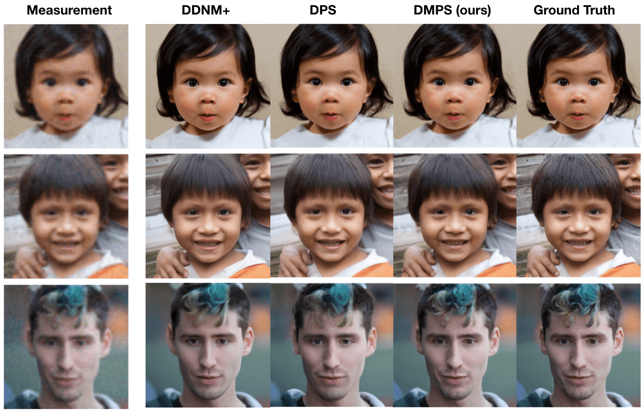
(a) Super-resolution (SR) ($\times 4$)

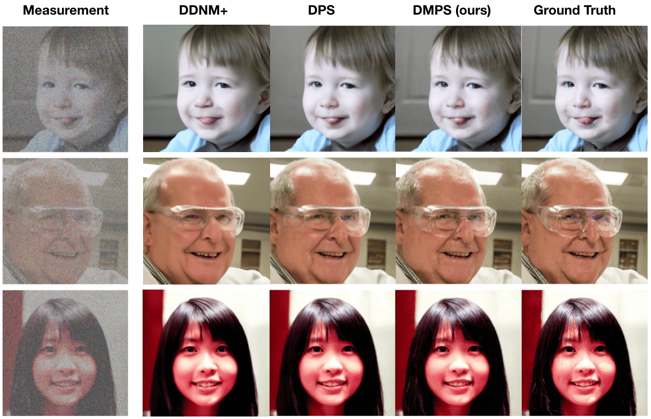
(b) Denoising ($\sigma=0.5$)

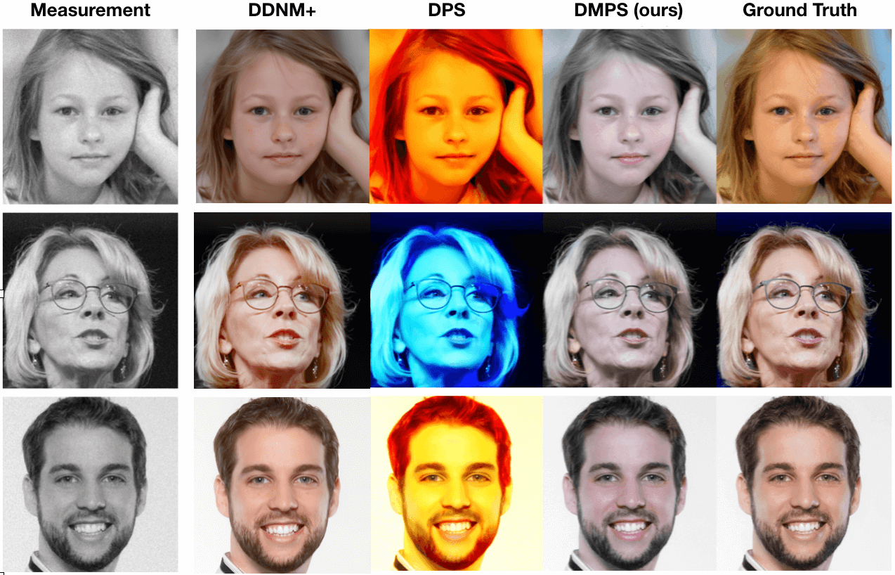
(c) colorization

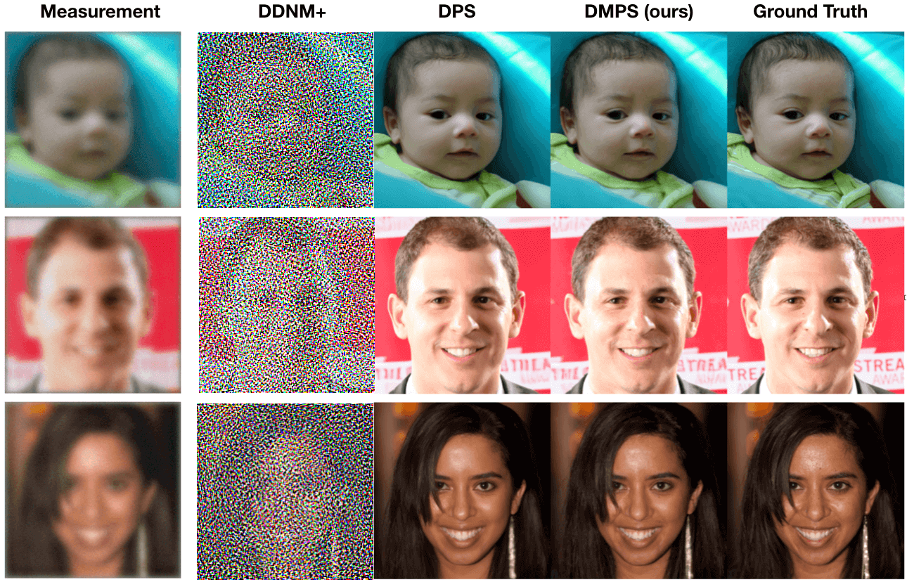
(d) Deblurring (uniform)

Figure 1: Typical results on FFHQ $256\times 256$ 1k validation set for different noisy linear inverse problems. In all cases, the measurements are with Gaussian noise $\sigma=0.05$, except denoising where $\sigma=0.5$. For more results, refer to Appendix F.

II-D Comparisons with DPS and DDNM

Hereby we compare DMPS with both DPS [24] and DDNM [25], unveiling the intrinsic connections. For DMPS and DPS, the only difference lies in the different way of estimating $p({\bf{y}}\mid{{\bf{x}}}_{t})=\int p({\bf{y}}\mid{\bf{x}}_{0})p({\bf{x}}_{0}\mid{\bf{x}}_{t})d{\bf{x}}_{0}$. Specifically, DPS uses a Dirac point estimate $p({\bf{x}}_{0}\mid{\bf{x}}_{t})\approx\delta({\bf{x}}_{0}-\hat{{\bf{x}}}_{0}({\bf{x}}_{t}))$, where $\hat{{\bf{x}}}_{0}({\bf{x}}_{t})=\frac{{\bf{x}}_{t}}{\sqrt{{\bar{\alpha}}_{t}}}-\sqrt{\frac{1-{\bar{\alpha}}_{t}}{{{\bar{\alpha}}_{t}}}}{\rm{s}}_{\boldsymbol{\theta}}({\bf{x}}_{t},t)$ is an estimate of the posterior mean of $p({\bf{x}}_{0}\mid{\bf{x}}_{t})$. By contrast, in DMPS, we use $\hat{{\bf{x}}}_{0}({\bf{x}}_{t})=\frac{{\bf{x}}_{t}}{\sqrt{{\bar{\alpha}}_{t}}}-\sqrt{\frac{1-{\bar{\alpha}}_{t}}{{{\bar{\alpha}}_{t}}}}\bf{w},\bf{w}\sim\mathcal{N}(\bf{0,I})$, so that instead of a Dirac function, $p({\bf{x}}_{0}\mid{\bf{x}}_{t})\approx\mathcal{N}({\bf{x}}_{0};\frac{{\bf{x}}_{t}}{\sqrt{{\bar{\alpha}}_{t}}},\frac{1-{\bar{\alpha}}_{t}}{{{\bar{\alpha}}_{t}}}\bf{I})$. It can be seen that DPS disregards the uncertainty in $p({\bf{x}}_{0}\mid{\bf{x}}_{t})$ while DMPS not. Regarding its connection to DDNM, interestingly, as shown in Appendix B, in the noiseless case where $\sigma=0$, DMPS closely resembles the DDNM [25] so that DMPS can be viewed as an robust version of DDNM in the noisy case when $\sigma>0$.

III Experiments

III-A Experimental Setup

Tasks: The tasks we consider include image super-resolution (SR), denoising, deblurring, as well as image colorization. In particular: (a) for image super-resolution (SR), the bicubic downsampling is performed as [24]; (b) for deblurring, uniform blur of size $9\times 9$ [22] are considered; (c) for colorization, the grayscale image is obtained by averaging the red, green, and blue channels of each pixel [22]. For all tasks, additive Gaussian noise $\bf{n}$ with $\sigma=0.05$ is added except the denoising task where a larger noise $\bf{n}$ with $\sigma=0.5$ is added.

Dataset: Different datasets are considered: FFHQ [36], CelebA-HQ [37], LSUN bedroom [38], and LSUN cat [38].

Pre-trained Diffusion Models: For fair of comparison, we use the same pre-trained (unconditional) ADM model from [39], available in https://drive.google.com/file/d/117Y6Z6-Hg6TMZVIXMmgYbpZy7QvTXign/view, for all the different methods evaluated.

Comparison Methods: We compare DMPS with the following SOTA methods: Diffusion Posterior Sampling (DPS) [24], the enhanced denoising diffusion null-space model (DDNM+) [25], manifold constrained gradients (MCG) [23]. The naive DDNM is not included since it completely fails in the noisy case [25].

Metrics: Three widely used metrics are considered, including the standard distortion metric peak signal noise ratio (PSNR) (dB), as well as two popular perceptual metrics: Fréchet inception distance (FID) [27, 28] and Learned Perceptual Image Patch Similarity (LPIPS) [29].

For more details of the experimental setting, please refer to Appendix C. The code to reproduce our results can be found in https://github.com/mengxiangming/dmps. All results are run on a single NVIDIA Tesla V100.

Results: We conducted experiments on both in-distribution FFHQ 1k validation dataset and out-of-distribution (OOD) samples from the CelebA-HQ 1k validation dataset. For DMPS pre-trained on LSUN bedroom and LSUN cat, we verify the efficacy of DMPS using OOD samples from the internet of the considered LSUN category. Due to the space limitation, only in-distribution results are shown in the main text while those for OOD samples are provided in Appendix E.

First, a quantitative comparison in terms of different metrics is shown in Table I. As shown in Table I, despite its simplicity, the proposed DMPS achieves highly competitive performances in multiple tasks and obtains a better perception-distortion tradeoff [40]. A qualitative comparison is shown in Fig. 1. In all tasks, DMPS produces high-quality realistic images which match details of the ground-truth more closely. For example, please have a look at the ear stud in the first row of Fig. 1 (a), the hand on the shoulder in the second row of Fig. 1 (a), the background in the second row of Fig. 1 (a), the hair style and bear in the third row of Fig. 1 (a); the background door in the first row of Fig. 1 (b), and the collar in the second row of Fig. 1 (b), etc. In addition, DPS tends to produce over-bright images in colorization while DMPS produces colored images in a more natural and realistic manner, i.e., closer to the ground-truth images, as shown in Fig. 1 (c). DDNM+ is also very competitive especially for colorization, but it is still senstive to noise, in particular for deblurring (see Fig. 1 (d)). More results can be found in Appendix F.

Moreover, we compare the running time of different algorithms. For fair of comparison, the average running time for one single function evaluation, i.e., the number of function evaluation (NFE) is one, is computed. As shown in Table II, DMPS is about three times faster than DPS.

Method	Running time for one single function evaluation [ms]
DMPS (ours)	67.02
DPS [24]	194.42
DDNM+ [25]	185.02
MCG [23]	193.71

TABLE II: Average running time per function evaluation (NFE = 1). This result is obtained on the SR task averaged for one single FFHQ $256\times 256$ sample.

IV Discussion and Conclusion

In this paper, to address the ubiquitous noisy linear inverse problem with the powerful diffusion models, a simple yet effective closed-form approximation of the intractable noise-perturbed likelihood score is proposed, leading to the diffusion model based posterior sampling (dubbed DMPS), a general-purpose inference method for a variety of linear inverse problems. With a specific focus on the ablated diffusion model (ADM), we evaluate the effectiveness of the proposed DMPS on multiple linear inverse problems including image super-resolution, denoising, deblurring, colorization. Remarkably, despite its simplicity, DMPS achieves highly competitive or even better performances in multiple tasks than the leading SOTA DPS [24], while the running time of DMPS is about $3\times$ faster than DPS.

Limitations $\&$ Future Work: While DMPS achieves excellent performances compared to SOTA methods, it still suffers several limitations. First, although memory efficient SVD exists for most practical matrices $\bf{A}$ of practical interests [22], the SVD operation in DMPS still has some implementation difficulty for more general matrices $\bf{A}$. Second, it can not be directly applied to the popular latent diffusion models such as stable diffusion [17], which is widely used due to its efficiency. Addressing these limitations are left as future work.

Appendix A Verification of Assumption 1

While the uninformative prior Assumption 1 appears crude at first sight, it is asymptotically accurate when the perturbed noise in ${\bf{x}}_{t}$ becomes negligible, which is the case in early phases of the forward diffusion process, i.e., $t$ is small. Since in general the exact likelihood $p({\bf{x}}_{0}\mid{\bf{x}}_{t})$ in (9) is intractable, it is generally difficult to exactly evaluate the effectiveness of Assumption 1. Instead, in the following we consider a toy example where the exact form of $p({\bf{x}}_{0}\mid{\bf{x}}_{t})$ in (9) can be computed exactly.

A toy example: Consider the case where $\bf{x}$ reduces to a scalar random variable $x$ and the associated prior $p(x)$ follows a Gaussian distribution, i.e., $p(x)=\mathcal{N}(x;0,\sigma^{2}_{0})$, where $\sigma^{2}$ is the prior variance. The likelihood $p({\bf{x}}_{t})|{\bf{x}}_{0})$ (4) in this case is simply $p({{x}}_{t}|{{x}}_{0})=\mathcal{N}({x_{t}};\sqrt{{\bar{\alpha}}_{t}}x_{0},(1-\bar{\alpha}_{t}))$.

Then, from (9), after some algebra, it can be computed that the posterior distribution $p({{x}}_{0}\mid{{x}_{t}})$ is

$$p({{x}_{0}}\mid{{x}_{t}})=\mathcal{N}({x}_{0};m_{\textrm{exact}},v_{\textrm{exact}})$$ (17)

where

$$m_{\textrm{exact}}=\frac{\sqrt{{\bar{\alpha}}_{t}}\sigma_{0}^{2}}{(1-{\bar{\alpha}}_{t})+{\bar{\alpha}}_{t}\sigma^{2}_{0}}{x}_{t},\;v_{\textrm{exact}}=\frac{(1-{\bar{\alpha}}_{t})\sigma^{2}_{0}}{(1-{\bar{\alpha}}_{t})+{\bar{\alpha}}_{t}\sigma^{2}_{0}}.$$ (18)

Under the Assumption 1, i.e., $p({{x}_{0}}|{{x}_{t}})\propto p({{x}_{t}}|{{x}_{0}})$, we obtain an approximation of $p({{x}}|{{x}_{t}})$ as follows

$$p({{x}_{0}}\mid{{x}_{t}})\simeq\tilde{p}({{x}_{0}}\mid{{x}_{t}})=\mathcal{N}({x}_{0};m_{\textrm{pseudo}},v_{\textrm{pseudo}}),$$ (19)

where

$$m_{\textrm{pseudo}}=\frac{1}{\sqrt{{\bar{\alpha}}_{t}}}{x}_{t},\;v_{\textrm{pseudo}}=\frac{1-{{\bar{\alpha}}_{t}}}{\bar{\alpha}}.$$ (20)

By comparing the exact result (18) and approximation result (20), it can be easily seen that for a fixed $\sigma^{2}_{0}>0$, as $\bar{\alpha}_{t}\to 1$, we have $m_{\textrm{pseudo}}\to m_{\textrm{post}}$ and $v_{\textrm{pseudo}}\to v_{\textrm{post}}$, which is exactly the case for DDPM as $t\to 1$. To see this, we anneal $\bar{\alpha}_{t}$ as $\bar{\alpha}_{t}={\bar{\alpha}}_{\rm{max}}(\frac{{\bar{\alpha}}_{\rm{min}}}{{\bar{\alpha}}_{\rm{max}}})^{\frac{t-1}{T-1}}$ geometrically and compare $m_{\textrm{pseudo}},v_{\textrm{pseudo}}$ with $m_{\textrm{exact}},v_{\textrm{exact}}$ as $t$ increase from $1$ to $T$. Assume that ${\bar{\alpha}}_{\rm{min}}=0.01$ and ${\bar{\alpha}}_{\rm{min}}=0.99$, and $\sigma_{0}=25,x_{t}=5,T=500$, we obtain the results in Fig. 2. It can be seen in Fig. 2 that the approximated values $m_{\textrm{pseudo}},v_{\textrm{pseudo}}$, especially the variance $v_{\textrm{pseudo}}$, approach to the exact values $m_{\textrm{exact}},v_{\textrm{exact}}$ very quickly, verifying the effectiveness of the Assumption 1 under this toy example.

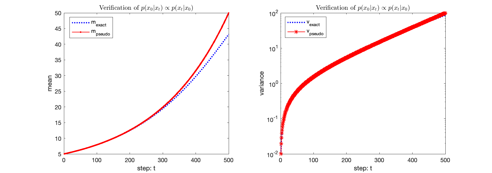
Figure 2: Comparison of the exact mean and variance of $p({{x}}_{0}\mid{{x}_{t}})$ with the pseudo mean and variance under the uninformative assumption, i.e., $p({{x}_{0}}\mid{{x}_{t}})\propto p({{x}}_{t}\mid{{x}_{0}})$ in the toy scalar Gaussian example. In this plot, we set ${\bar{\alpha}}_{\rm{min}}=0.01$ and ${\bar{\alpha}}_{\rm{min}}=0.99$, and $\sigma_{0}=25,x_{t}=5,T=500$. It can be seen that the approximated pseudo values approach the exact values very quickly as $t$ becomes smaller, verifying the effectiveness of the Assumption 1 for this toy example.

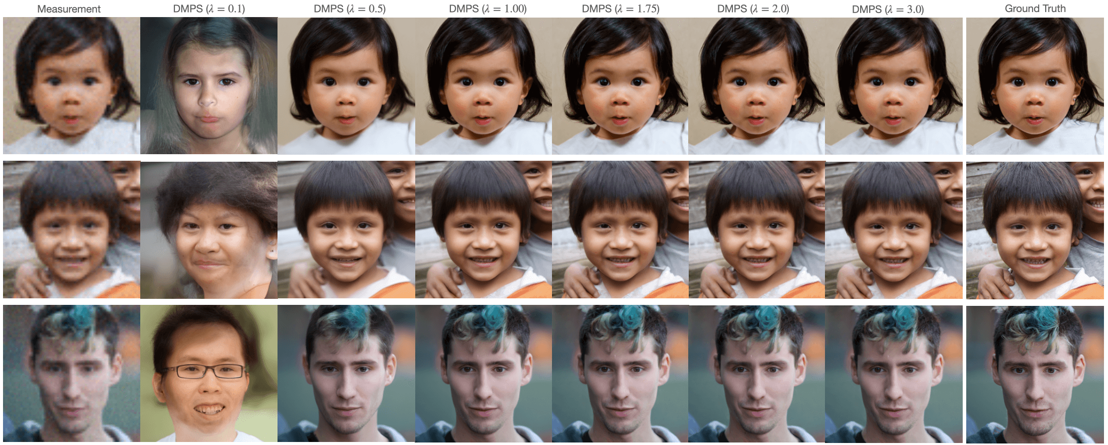
Figure 3: Results of DMPS with different $\lambda$ for the task of noisy SR ($\times 4$) with $\sigma=0.05$. It can be seen that DMPS is very robust to different choices of $\lambda$, i.e., it works very well in a wide range of values.

Appendix B Connection to DDNM

Interestingly, in the special noiseless case, i.e., $\sigma=0$, the proposed DMPS reduces to a form that closely resembles DDNM [25]. Specifically, from (10), when $\sigma=0$, we have

$$\nabla_{{\bf{x}}_{t}}\log{p({\bf{y}}\mid{\bf{x}}_{t}})\simeq\nabla_{{\bf{x}}_{t}}\log{{\tilde{p}}({\bf{y}}\mid{\bf{x}}_{t}})$$

$$= \frac{\sqrt{\bar{\alpha}}_{t}}{{1-{\bar{\alpha}}_{t}}}{\bf{A}}^{+}\big{(}{\bf{y}}-\frac{1}{\sqrt{{\bar{\alpha}}_{t}}}{{\bf{A{\bf{x}}}}_{t}}\big{)},$$ (21)

where ${\bf{A}}^{+}={\bf{A}}^{T}{({\bf{A}}{\bf{A}}^{T})^{-1}}$ is the pseudo-inverse of ${\bf{A}}$ when ${\bf{A}}$ has linearly independent rows. As a result, from Algorithm 1, the resultant iterative step becomes

$${\bf{x}}_{t-1} =\frac{1}{\sqrt{\alpha_{t}}}\big{(}{\bf{x}}_{t}-\frac{1-\alpha_{t}}{\sqrt{1-\bar{\alpha}}_{t}}{\rm{s}}_{\boldsymbol{\theta}}({\bf{x}}_{t},t)\big{)}+\tilde{\sigma}_{t}{\bf{z}}_{t}+{\lambda\frac{1-\alpha_{t}}{\sqrt{\alpha_{t}}}\frac{\sqrt{\bar{\alpha}}_{t}}{{1-{\bar{\alpha}}_{t}}}{\bf{A}}^{+}\big{(}{\bf{y}}-\frac{1}{\sqrt{{\bar{\alpha}}_{t}}}{{\bf{A{\bf{x}}}}_{t}}\big{)}}.$$ (22)

In DDNM, from the Algorithm 1 in [25], the resultant iterative step can be written as follows

$$\mathbf{x}_{t-1} =\frac{\sqrt{\bar{\alpha}_{t-1}}\beta_{t}}{1-\bar{\alpha}_{t}}\hat{\mathbf{x}}_{0|t}+\frac{\sqrt{\alpha_{t}}(1-\bar{\alpha}_{t-1})}{1-\bar{\alpha}_{t}}\mathbf{x}_{t}+\tilde{\sigma}_{t}\mathbf{z}_{t}$$

$$=\frac{\sqrt{{\bar{\alpha}}_{t-1}}\beta_{t}}{1-\bar{\alpha}_{t}}\mathbf{x}_{0|t}+\frac{\sqrt{{{\alpha}}_{t}}(1-\bar{\alpha}_{t-1})}{1-\bar{\alpha}_{t}}\mathbf{x}_{t}+\tilde{\sigma}_{t}\mathbf{z}_{t}+\frac{\sqrt{{\bar{\alpha}}_{t-1}}\beta_{t}}{1-\bar{\alpha}_{t}}{\bf{A}}^{+}\big{(}{\bf{y}}-\mathbf{Ax}_{0|t}\big{)}$$

$$=\frac{1}{\sqrt{\alpha_{t}}}\big{(}{\bf{x}}_{t}-\frac{1-\alpha_{t}}{\sqrt{1-\bar{\alpha}}_{t}}{\rm{s}}_{\boldsymbol{\theta}}({\bf{x}}_{t},t)\big{)}+\tilde{\sigma}_{t}\mathbf{z}_{t}+\frac{\sqrt{{\bar{\alpha}}_{t-1}}\beta_{t}}{1-\bar{\alpha}_{t}}{\bf{A}}^{+}\big{(}{\bf{y}}-\frac{1}{\sqrt{{\bar{\alpha}}_{t}}}{{\bf{A{\bf{x}}}}_{t}}\color[rgb]{0,0,1}{+\sqrt{\frac{1-\bar{\alpha}_{t}}{\bar{\alpha}_{t}}}{\bf{A}}{\rm{s}}_{\boldsymbol{\theta}}({\bf{x}}_{t},t)}\big{)}.$$ (23)

Comparing (22) with (23), it can be seen that DMPS in the special case of $\sigma=0$ has a similar form as that of DDNM, except that the blue part in (22) and (23) are slightly different. In particular, when the scaling factor $\lambda$ is set to be $\lambda=\sqrt{\frac{\alpha_{t}\bar{\alpha}_{t-1}}{\bar{\alpha}_{t}}}$, the update equation of DMPS in (22)becomes

$${\bf{x}}_{t-1} =\frac{1}{\sqrt{\alpha_{t}}}\big{(}{\bf{x}}_{t}-\frac{1-\alpha_{t}}{\sqrt{1-\bar{\alpha}}_{t}}{\rm{s}}_{\boldsymbol{\theta}}({\bf{x}}_{t},t)\big{)}+\tilde{\sigma}_{t}{\bf{z}}_{t}+{\frac{\sqrt{{\bar{\alpha}}_{t-1}}\beta_{t}}{1-\bar{\alpha}_{t}}{\bf{A}}^{+}\big{(}{\bf{y}}-\frac{1}{\sqrt{{\bar{\alpha}}_{t}}}{{\bf{A{\bf{x}}}}_{t}}\big{)}},$$ (24)

which differs with DDNM solely with a lack of the term $\sqrt{\frac{1-\bar{\alpha}_{t}}{\bar{\alpha}_{t}}}{\bf{A}}{\rm{s}}_{\boldsymbol{\theta}}({\bf{x}}_{t},t)$. In fact, as ${\rm{s}}_{\boldsymbol{\theta}}({\bf{x}}_{t},t)$ essentially approximate a Gaussian noise with zero mean. As a result, the mean value of $\sqrt{\frac{1-\bar{\alpha}_{t}}{\bar{\alpha}_{t}}}{\bf{A}}{\rm{s}}_{\boldsymbol{\theta}}({\bf{x}}_{t},t)$ is zero, so that DDNM keeps its original form $\big{(}{\bf{y}}-\mathbf{Ax}_{0|t}\big{)}$ while DMPS uses the mean value of it. For the noisy case where $\sigma>0$, DMPS can be viewed as an improvement of DDNM by explicitly considering the noise.

Appendix C Detailed Experimental Settings

Datasets: For DMPS pre-trained on FFHQ, similar to [24], we conducted experiments on both the in-distribution FFHQ 1k validation dataset and OOD samples from the CelebA-HQ $256\times 256$-1k validation dataset. For DMPS with pre-trained on LSUN bedroom and LSUN cat [38], similar to [22], we verify the efficacy of DMPS using OOD samples from the internet of the considered LSUN category, respectively.

Comparison Methods: We compare DMPS with the following SOTA methods based on DM: Diffusion Posterior Sampling (DPS) [24], the enhanced denoising diffusion null-space model (DDNM+) [25], and manifold constrained gradients (MCG) [23]. The results of other methods such as SNIPS [21], PnP-ADMM[41] and Score-SDE [42] are not shown as they have been demonstrated to be apparently inferior to DPS on similar tasks [24, 22]. For fair of comparison, all the methods use exactly the same pre-trained models. The associated hyper-parameters of DPS, MCG are set as their default values. For our DMPS, we run all the experiments with fixed $\lambda=1.75$ though it is believed a task-specific fine-tuning can further improve the performance. For details, please refer to their open-sourced codes.

Metrics: The PSNR and LPIPS are computed using the open-sourced code in [24], which is available at https://github.com/DPS2022/diffusion-posterior-sampling. The FID are computed between the reconstructed images and the ground-truth images using the Pytorch code provided in [28], which is available at https://github.com/mseitzer/pytorch-fid.

Appendix D Effect of Scaling Parameter $\lambda$

As shown in Algorithm 1, a hyper-parameter $\lambda$ is introduced as a scaling value for the likelihood score. Empirically it is found that DMPS is robust to different choices of $\lambda$ around 1 though most of the time $\lambda>1$ yields slightly better results. As one specific example, we show the results of DMPS for super-resolution (SR $\times 4$) for different values of $\lambda$, as shown in Fig. 3. It can be seen that DMPS is very robust to different choices of $\lambda$, i.e., it works very well in a wide range of values.

Appendix E OOD Results

In practice, the target $\bf{x}$ might be out-of-distribution (OOD) since the available training dataset has bias and thus cannot exactly match the true underlying distribution $p(\bf{x})$. Therefore, it is essential to assess the generalization performance on OOD samples. The results on OOD samples are shown in Table III and Fig. 4.

SR ($\times 4$) Denoise Colorization Deblur (uniform) Method PSNR $\uparrow$ FID $\downarrow$ LPIPS $\downarrow$ PSNR $\uparrow$ FID $\downarrow$ LPIPS $\downarrow$ PSNR $\uparrow$ FID $\downarrow$ LPIPS $\downarrow$ PSNR $\uparrow$ FID $\downarrow$ LPIPS $\downarrow$ DMPS (ours) 28.24 28.13 0.2128 28.40 41.35 0.2663 21.42 43.75 0.2932 27.86 33.38 0.2407 DPS 27.41 36.27 0.2374 27.71 37.09 0.2502 12.23 86.27 0.5439 27.13 35.55 0.2414 DDNM+ 29.23 38.88 0.2443 27.84 41.72 0.2726 25.14 30.10 0.2583 6.275 417.7 0.8616 MCG 18.11 214.3 0.6727 27.86 69.35 0.2471 12.01 126.8 0.5439 10.67 362.2 0.7862

TABLE III: Quantitative comparison (PSNR (dB), FID, LPIPS) of different algorithms for different tasks on the OOD CelebA-HQ $256\times 256$-1k validation dataset. The DM used in DMPS, DPS, DDNM+, MCG is the same and is trained on FFHQ.

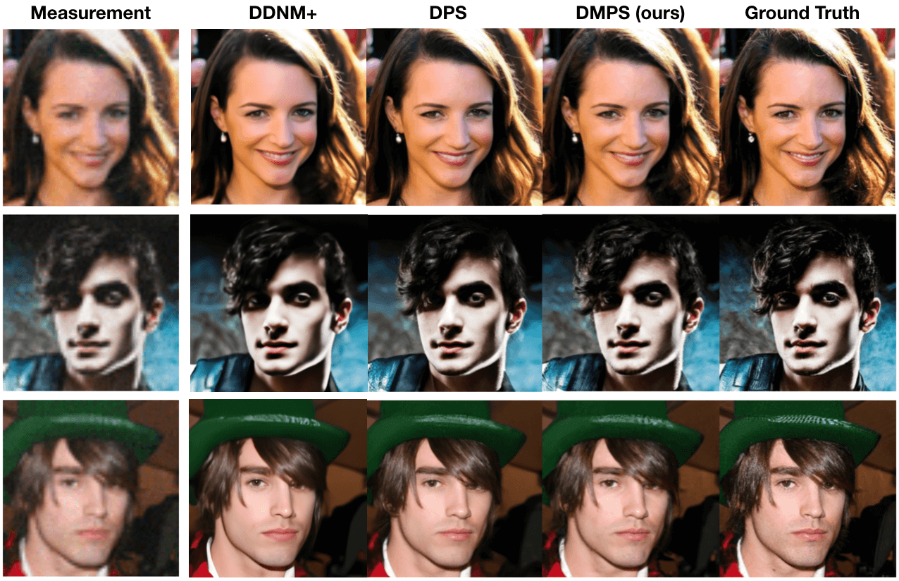
(a) Super-resolution (SR) ($\times 4$), OOD CelebA-HQ

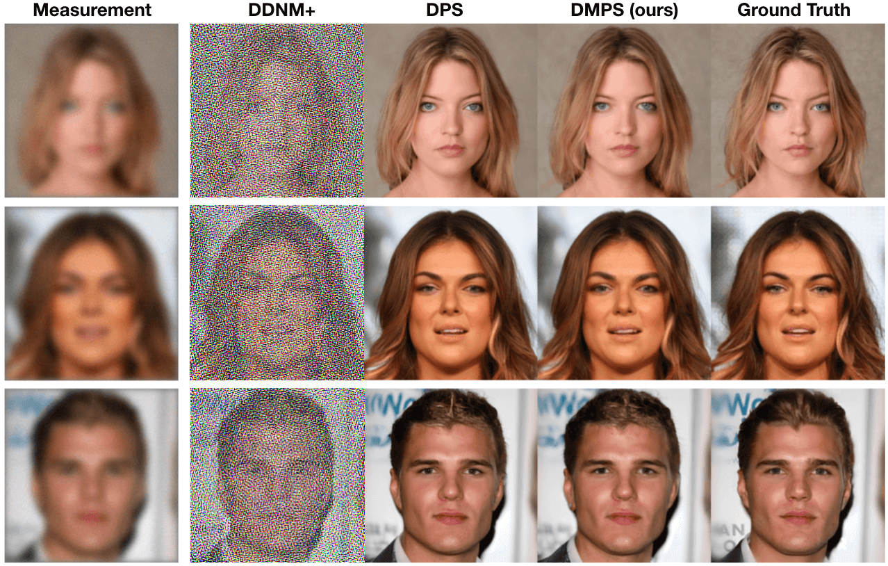
(b) Deblurring (Gaussian), OOD CelebA-HQ

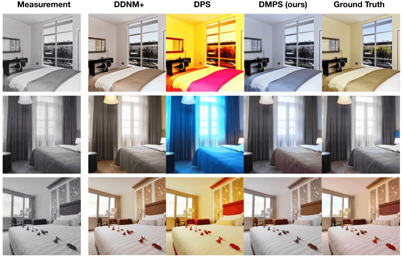
(c) Colorization, OOD bedroom

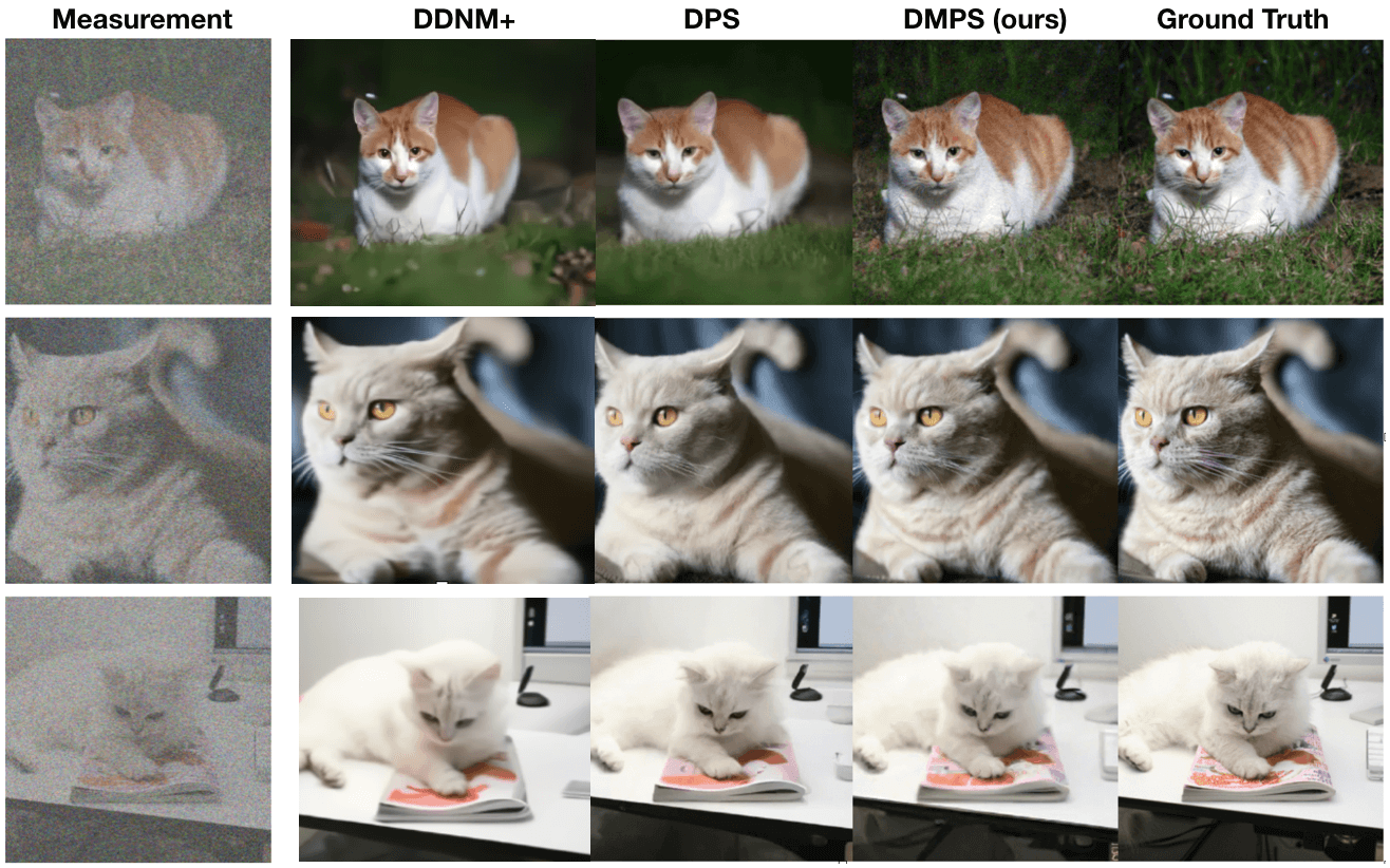
(d) Denoising ($\sigma=0.5$), OOD cat

Figure 4: Typical results on OOD samples, including $256\times 256$ CelebA-HQ, OOD bedroom, OOD cat, for different noisy linear inverse problems. For more results, refer to Appendix F.

Appendix F Additional Results

Finally, we show some additional results of DMPS for differet tasks on FFHQ $256\times 256$ 1k validation set in Fig. 5, Fig. 6, Fig. 7, and Fig. 8.

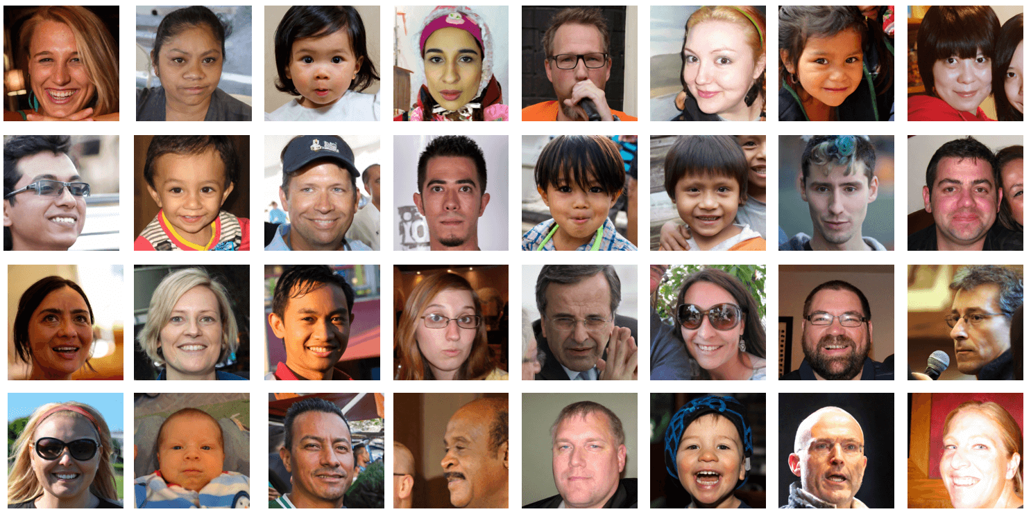
(a) Recovered results of DMPS (ours)

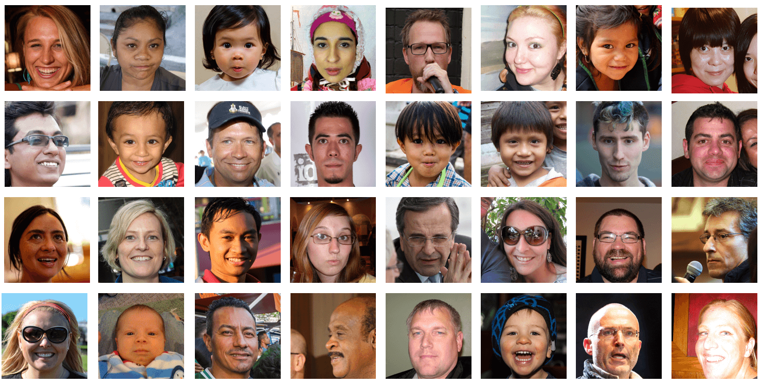
(b) Ground Truth

Figure 5: Additional results of DMPS on FFHQ $256\times 256$ 1k validation set for super-resolution (SR) ($\times 4$), $\sigma=0.05$.

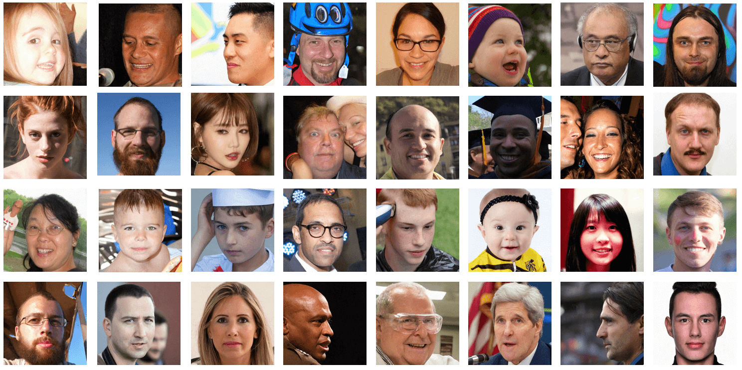
(a) Recovered results of DMPS (ours)

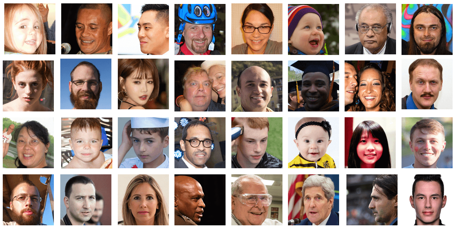
(b) Ground Truth

Figure 6: Additional results of DMPS on FFHQ $256\times 256$ 1k validation set for denoising ($\sigma=0.5$).

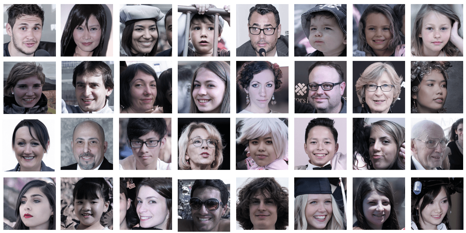
(a) Recovered results of DMPS (ours)

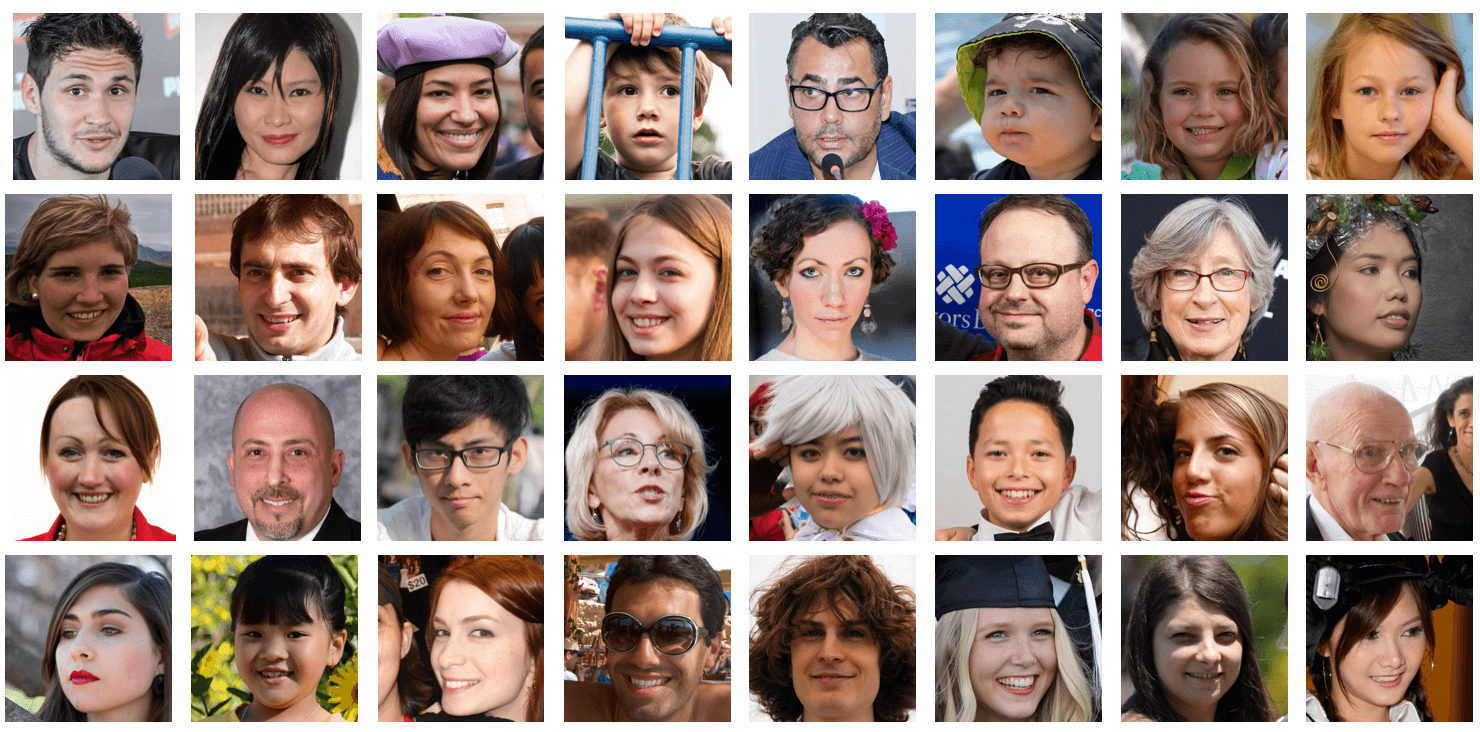
(b) Ground Truth

Figure 7: Additional results of DMPS on FFHQ $256\times 256$ 1k validation set for colorization, $\sigma=0.05$.

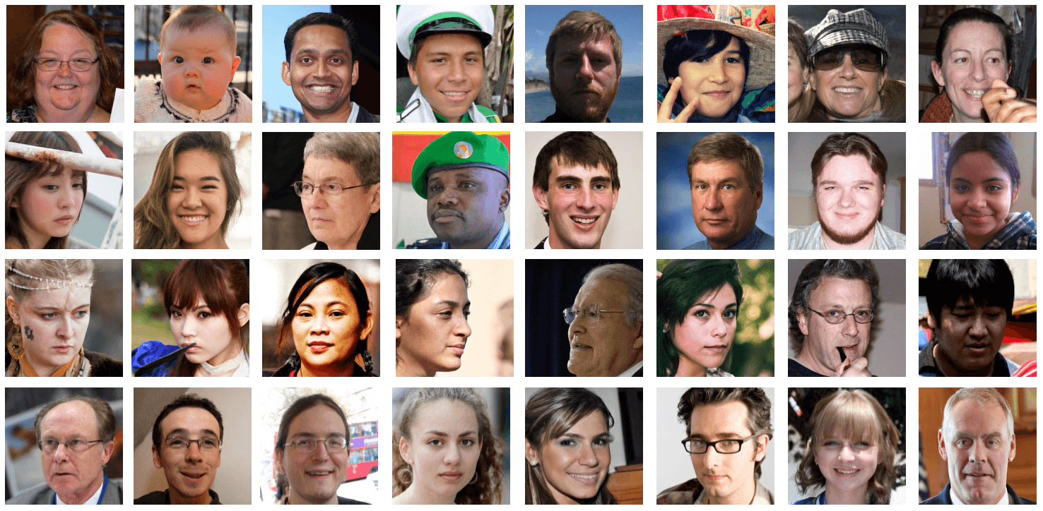
(a) Recovered results of DMPS (ours)

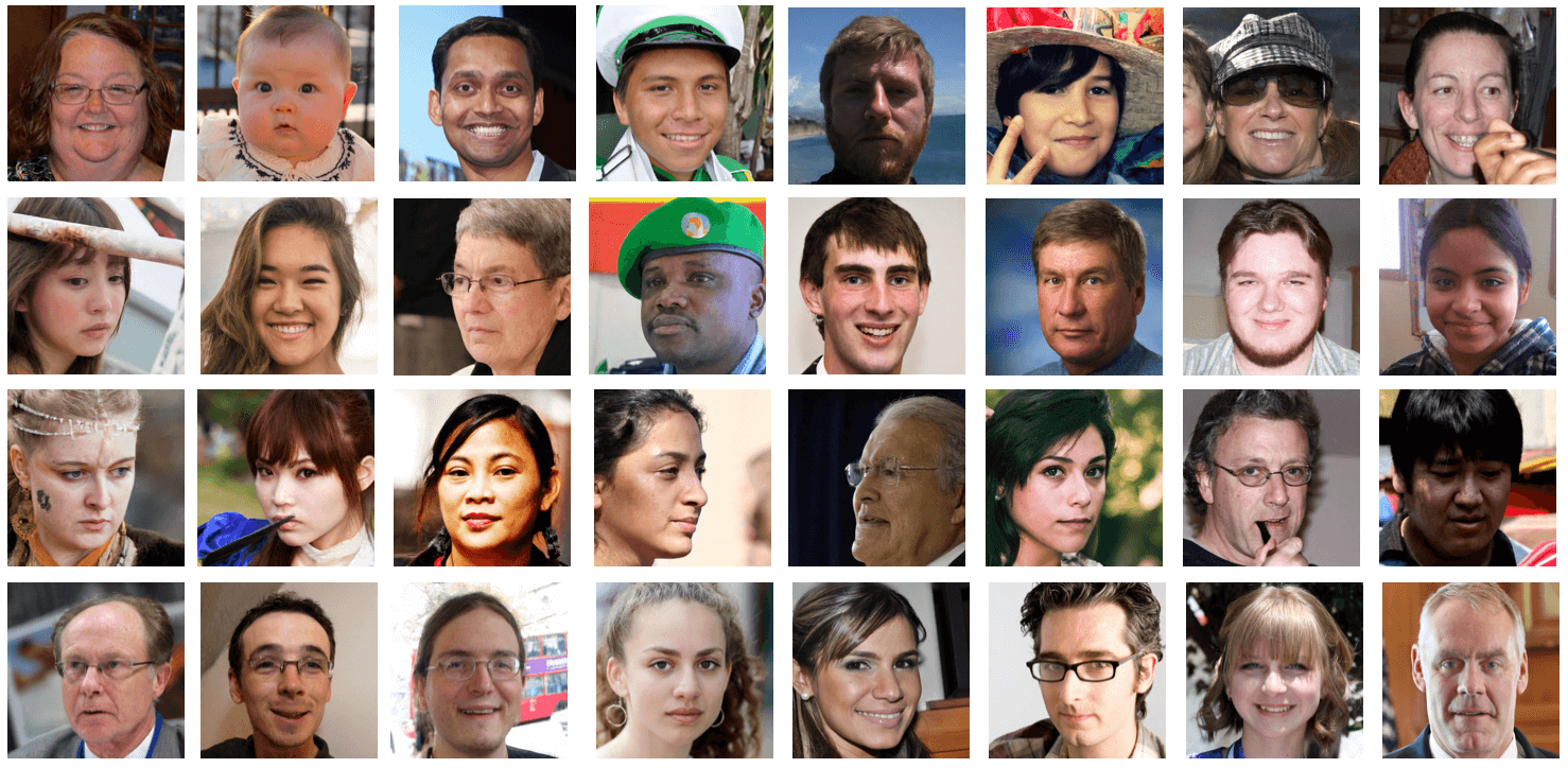
(b) Ground Truth

Figure 8: Additional results of DMPS on FFHQ $256\times 256$ 1k validation set for deblurring (uniform), $\sigma=0.05$.

References

- [1] C. Ledig, L. Theis, F. Huszár, J. Caballero, A. Cunningham, A. Acosta, A. Aitken, A. Tejani, J. Totz, Z. Wang et al., “Photo-realistic single image super-resolution using a generative adversarial network,” in Proceedings of the IEEE conference on computer vision and pattern recognition, 2017, pp. 4681–4690.
- [2] R. Zhang, P. Isola, and A. A. Efros, “Colorful image colorization,” in European conference on computer vision. Springer, 2016, pp. 649–666.
- [3] A. Buades, B. Coll, and J.-M. Morel, “A review of image denoising algorithms, with a new one,” Multiscale modeling & simulation, vol. 4, no. 2, pp. 490–530, 2005.
- [4] L. Yuan, J. Sun, L. Quan, and H. Shum, “Image deblurring with blurred/noisy image pairs,” in Proceedings of the 34th ACM SIGGRAPH Conference on Computer Graphics, 34th Annual Meeting of the Association for Computing Machinery’s Special Interest Group on Graphics; San Diego, CA; United States, 2007.
- [5] M. Bertalmio, G. Sapiro, V. Caselles, and C. Ballester, “Image inpainting,” in Proceedings of the 27th annual conference on Computer graphics and interactive techniques, 2000, pp. 417–424.
- [6] E. J. Candès, J. Romberg, and T. Tao, “Robust uncertainty principles: Exact signal reconstruction from highly incomplete frequency information,” IEEE Transactions on information theory, vol. 52, no. 2, pp. 489–509, 2006.
- [7] E. J. Candès and M. B. Wakin, “An introduction to compressive sampling,” IEEE signal processing magazine, vol. 25, no. 2, pp. 21–30, 2008.
- [8] F. O’Sullivan, “A statistical perspective on ill-posed inverse problems,” Statistical science, pp. 502–518, 1986.
- [9] M. Fazel, E. Candes, B. Recht, and P. Parrilo, “Compressed sensing and robust recovery of low rank matrices,” in 2008 42nd Asilomar Conference on Signals, Systems and Computers. IEEE, 2008, pp. 1043–1047.
- [10] D. Ulyanov, A. Vedaldi, and V. Lempitsky, “Deep image prior,” in Proceedings of the IEEE conference on computer vision and pattern recognition, 2018, pp. 9446–9454.
- [11] I. Goodfellow, J. Pouget-Abadie, M. Mirza, B. Xu, D. Warde-Farley, S. Ozair, A. Courville, and Y. Bengio, “Generative adversarial nets,” in Advances in Neural Information Processing Systems, vol. 27. Curran Associates, Inc., 2014.
- [12] D. P. Kingma and M. Welling, “Auto-encoding variational bayes,” arXiv preprint arXiv:1312.6114, 2013.
- [13] J. Sohl-Dickstein, E. Weiss, N. Maheswaranathan, and S. Ganguli, “Deep unsupervised learning using nonequilibrium thermodynamics,” in International Conference on Machine Learning. PMLR, 2015, pp. 2256–2265.
- [14] Y. Song and S. Ermon, “Generative modeling by estimating gradients of the data distribution,” Advances in Neural Information Processing Systems, vol. 32, 2019.
- [15] J. Ho, A. Jain, and P. Abbeel, “Denoising diffusion probabilistic models,” Advances in Neural Information Processing Systems, vol. 33, pp. 6840–6851, 2020.
- [16] P. Dhariwal and A. Nichol, “Diffusion models beat gans on image synthesis,” Advances in Neural Information Processing Systems, vol. 34, pp. 8780–8794, 2021.
- [17] R. Rombach, A. Blattmann, D. Lorenz, P. Esser, and B. Ommer, “High-resolution image synthesis with latent diffusion models,” in Proceedings of the IEEE/CVF Conference on Computer Vision and Pattern Recognition, 2022, pp. 10 684–10 695.
- [18] A. Bora, A. Jalal, E. Price, and A. G. Dimakis, “Compressed sensing using generative models,” in International Conference on Machine Learning. PMLR, 2017, pp. 537–546.
- [19] A. Jalal, M. Arvinte, G. Daras, E. Price, A. G. Dimakis, and J. Tamir, “Robust compressed sensing mri with deep generative priors,” Advances in Neural Information Processing Systems, vol. 34, pp. 14 938–14 954, 2021.
- [20] A. Jalal, S. Karmalkar, A. Dimakis, and E. Price, “Instance-optimal compressed sensing via posterior sampling,” in International Conference on Machine Learning. PMLR, 2021, pp. 4709–4720.
- [21] B. Kawar, G. Vaksman, and M. Elad, “Snips: Solving noisy inverse problems stochastically,” Advances in Neural Information Processing Systems, vol. 34, pp. 21 757–21 769, 2021.
- [22] B. Kawar, M. Elad, S. Ermon, and J. Song, “Denoising diffusion restoration models,” arXiv preprint arXiv:2201.11793, 2022.
- [23] H. Chung, B. Sim, D. Ryu, and J. C. Ye, “Improving diffusion models for inverse problems using manifold constraints,” arXiv preprint arXiv:2206.00941, 2022.
- [24] H. Chung, J. Kim, M. T. Mccann, M. L. Klasky, and J. C. Ye, “Diffusion posterior sampling for general noisy inverse problems,” arXiv preprint arXiv:2209.14687, 2022.
- [25] Y. Wang, J. Yu, and J. Zhang, “Zero-shot image restoration using denoising diffusion null-space model,” arXiv preprint arXiv:2212.00490, 2022.
- [26] X. Meng and Y. Kabashima, “Quantized compressed sensing with score-based generative models,” in International Conference on Learning Representations, 2023.
- [27] M. Heusel, H. Ramsauer, T. Unterthiner, B. Nessler, and S. Hochreiter, “Gans trained by a two time-scale update rule converge to a local nash equilibrium,” Advances in neural information processing systems, vol. 30, 2017.
- [28] M. Seitzer, “pytorch-fid: FID Score for PyTorch,” https://github.com/mseitzer/pytorch-fid, August 2020, version 0.2.1.
- [29] R. Zhang, P. Isola, A. A. Efros, E. Shechtman, and O. Wang, “The unreasonable effectiveness of deep features as a perceptual metric,” in Proceedings of the IEEE conference on computer vision and pattern recognition, 2018, pp. 586–595.
- [30] R. Tibshirani, “Regression shrinkage and selection via the lasso,” Journal of the Royal Statistical Society: Series B (Methodological), vol. 58, no. 1, pp. 267–288, 1996.
- [31] A. Beck and M. Teboulle, “A fast iterative shrinkage-thresholding algorithm for linear inverse problems,” SIAM journal on imaging sciences, vol. 2, no. 1, pp. 183–202, 2009.
- [32] J. A. Tropp and S. J. Wright, “Computational methods for sparse solution of linear inverse problems,” Proceedings of the IEEE, vol. 98, no. 6, pp. 948–958, 2010.
- [33] Y. Kabashima, “A cdma multiuser detection algorithm on the basis of belief propagation,” Journal of Physics A: Mathematical and General, vol. 36, no. 43, p. 11111, 2003.
- [34] D. L. Donoho, A. Maleki, and A. Montanari, “Message-passing algorithms for compressed sensing,” Proceedings of the National Academy of Sciences, vol. 106, no. 45, pp. 18 914–18 919, 2009.
- [35] Y. Song, P. Dhariwal, M. Chen, and I. Sutskever, “Consistency models,” arXiv preprint arXiv:2303.01469, 2023.
- [36] T. Karras, S. Laine, and T. Aila, “A style-based generator architecture for generative adversarial networks,” in Proceedings of the IEEE/CVF conference on computer vision and pattern recognition, 2019, pp. 4401–4410.
- [37] T. Karras, T. Aila, S. Laine, and J. Lehtinen, “Progressive growing of gans for improved quality, stability, and variation,” in International Conference on Learning Representations, 2018.
- [38] F. Yu, A. Seff, Y. Zhang, S. Song, T. Funkhouser, and J. Xiao, “Lsun: Construction of a large-scale image dataset using deep learning with humans in the loop,” arXiv preprint arXiv:1506.03365, 2015.
- [39] J. Choi, S. Kim, Y. Jeong, Y. Gwon, and S. Yoon, “Ilvr: Conditioning method for denoising diffusion probabilistic models,” in 2021 IEEE/CVF International Conference on Computer Vision (ICCV). IEEE, 2021, pp. 14 347–14 356.
- [40] Y. Blau and T. Michaeli, “The perception-distortion tradeoff,” in Proceedings of the IEEE conference on computer vision and pattern recognition, 2018, pp. 6228–6237.
- [41] S. H. Chan, X. Wang, and O. A. Elgendy, “Plug-and-play admm for image restoration: Fixed-point convergence and applications,” IEEE Transactions on Computational Imaging, vol. 3, no. 1, pp. 84–98, 2016.
- [42] Y. Song, J. Sohl-Dickstein, D. P. Kingma, A. Kumar, S. Ermon, and B. Poole, “Score-based generative modeling through stochastic differential equations,” in International Conference on Learning Representations, 2020.