Hot subdwarf stars identified in LAMOST DR8 with single-lined and composite spectra

Abstract

222 hot subdwarf stars were identified with LAMOST DR8 spectra, among which 131 stars show composite spectra and have been decomposed, while 91 stars present single-lined spectra. Atmospheric parameters of all sample stars were obtained by fitting Hydrogen (H) and Helium (He) line profiles with synthetic spectra. Two long-period composite sdB binaries were newly discovered by combining our sample with the non-single star data from Gaia DR3. One of the new systems presents the highest eccentricity (i.e., $0.5\pm 0.09$) among known wide sdB binaries, which is beyond model predictions. 15 composite sdB stars fall in the high probability binary region of RUWE-AEN plane, and deserve priority follow-up observations to further study their binary nature. A distinct gap is clearly presented among temperatures of cool companions for our composite-spectra sample. But we could not come to a conclusion whether this feature is connected to the formation history of hot subdwarf stars before their binary natures are confirmed.

1 Introduction

Hot subdwarf stars have similar spectra as O/B type main-sequence (MS) stars, but at lower luminosity. They have low masses around at 0.5 M_⊙ but very high effective temperatures and surface gravity (e.g., roughly 20000 K $\leq$ $T_{\mathrm{eff}}$ $\leq$ 70000 K and 5.0 $\leq$ $\mathrm{log}\ g$ $\leq$ 6.5, see Heber 2009, 2016 for excellent review on this type of stars). Hot subdwarf stars are burning helium (He) in their cores or have evolved even off this stage. Many of these stars occupy the bluest positions at the end of the horizontal branch (HB) in the Hertzsprung-Russell (H-R) diagram, hence they are also known as extreme horizontal branch (EHB) stars, which show up most remarkably in globular clusters (GCs). Some other types of stars could also go across the hot subdwarf region in the H-R diagram (Heber, 1986, 2016), such as post-EHB stars, post asymptotic giant branch (post-AGB) stars, low and extremely low mass (pre-)white dwarfs (pre-ELM WDs), etc.

According to the characteristics of spectral lines, hot subdwarf stars can be classified into several sub types, e.g., sdB, sdOB, sdO, He-sdB, He-sdOB and He-sdO (Moehler et al., 1990; Geier et al., 2017). sdB stars have dominant H Balmer lines but weak or absent He lines. sdOB stars have dominant H Balmer lines, together with both weak He I and He II lines, while sdO stars present dominant H Balmer lines and an obvious He II line at 4686 Å, but without obvious He I lines. On the other hand, He-sdB stars show dominant He I lines, but weak or absent H Balmers and He II lines. He-sdOB stars present both strong He I and He II lines, but with weak or absent H Balmer lines, while He-sdO stars present strong He II lines, but weak or absent H Balmer lines and HeI lines.

Since many of hot subdwarfs were found in close binary systems, they are considered to be mainly formed in binary evolution. Han et al. (2002, 2003) conducted detailed binary population synthesis and found that stable Roche lobe overflow (RLOF), common envelope (CE) ejection and a merger of two He white dwarf (WD) stars in binary evolution are three main possible formation channels for sdB stars (also see Chen et al. 2013). Clausen & Wade (2011) proposed that the merger of an He WD with an M dwarf star can produce single sdB stars. This model could account for the narrow mass range of single sdB stars and the existence of long-period sdB+MS binaries. On the other hand, Zhang & Jeffery (2012) studied the merger of two He WDs in short orbital period, and found that both fast and slow accretion processes could reproduce He-rich hot subdwarf stars. Moreover, Zhang et al. (2017) also found that the merger of a He WD and a main-sequence star could contribute to the formation of intermediate He-rich subdwarfs. Lei et al. (2015, 2016) also found that tidally-enhanced stellar wind in binary evolution could contribute on the formation of blue hook (BHk) stars in GCs.

Long period composite sdB binaries are the result of the stable-RLOF formation channel. In fact, F/G/K type companions are only found in long period sdB binaries. Their existence was predicted by Green et al. (2001), but it had taken another decade until the first orbits of long period sdBs were published (Deca et al., 2012; Østensen & Van Winckel, 2012; Vos et al., 2012). Currently 23 composite sdB binaries have solved orbits. These systems are found with orbital periods ranging from 2 to well over 4 years, and their properties have several puzzling features (Vos et al., 2019). Tidal circularisation theory predicts the sdB progenitors to circularize completely before the interaction phase starts, however, most observed wide sdB binaries have eccentric orbits. The interaction with a circumbinary disk during the mass loss phase can explain many, but not all, of these eccentric systems (Vos et al., 2015). More recently a strong correlation between orbital period and mass-ratio was linked to the galactic metallicity evolution (Vos et al., 2020). Several other peculiarities, as for example the bimodal distribution in the period - mass ratio and period - eccentricity parameter space, remain unexplained. These composite sdBs are a valuable population to study binary interaction theories as the orbital properties and the spectral properties of both components can be solved, and because all systems form a single population.

From an observational point of view, with the huge data released from large photometric and spectroscopic surveys, new discoveries of hot subdwarf stars have increased very quickly in recent years. A catalog of known hot subdwarf stars was compiled from literature and reported by Geier et al. (2017), which contains 5613 objects and a lot of useful information, such as: multi-band photometry, ground based proper motions, classifications, published atmospheric parameters, etc. Kepler et al. (2019) confirmed 20 088 WDs, 425 hot subdwarfs, and 311 cataclysmic variables (CVs) based on the spectra released by Sloan Digital Sky Survey Data Release 14 (SDSS DR14, Abolfathi et al. 2018). On the other hand, the second data release of the Gaia mission (Gaia DR2) became available to the public in 2018, which provided precise astrometry and photometry for more than 1.3 billion sources over the full sky (Gaia Collaboration et al., 2018a). With this useful information, hot subdwarf candidates could be selected more efficiently and accurately in H-R diagram (Gaia Collaboration et al., 2018b). Based on Gaia DR2 data, Geier et al. (2019) compiled a candidates catalog by means of colour, absolute magnitude, and reduced proper motion cuts, in which 39 800 hot sub-luminous candidates were selected, and it proved as a good input catalog for large photometric and spectroscopic surveys for further study of hot subdwarfs. The number of candidates increased to 61 585 by Culpan et al. (2022) as new data was updated from Gaia EDR3 (Gaia Collaboration et al., 2021).

With the help of precise photometric magnitudes and parallaxes provided by Gaia DR2, more than 1000 hot subdwarfs were identified in The Large Sky Area Multi-Object Fiber Spectroscopic Telescope (LAMOST) spectral survey (Luo et al., 2019, 2021; Lei et al., 2018, 2019b, 2020), and reliable atmospheric parameters (e.g., effective temperature, gravity and He abundance) were obtained by fitting hydrogen (H) and He line profiles with synthetic spectra. Moreover, Geier (2020) compiled a new catalog with 5874 known hot subdwarf stars recorded, including 528 newly discovered objects and removing 268 previously misclassified objects with respect to the previous catalog of Geier et al. (2017).

On the other hand, artificial intelligence (AI) methods were widely used recently in research fields of astronomy and astrophysics, including searching for hot subdwarfs in large photometric and spectroscopic surveys. Bu et al. (2017) firstly selected about 7000 hot subdwarf candidates from the first data release (DR1) of LAMOST spectral survey, by employing a machine learning algorithm. Based on these candidates, Lei et al. (2019a) identified 56 hot subdwarf stars by detailed spectral analysis, and provided reliable atmospheric parameters. Subsequently, a deep learning method equipped by convolutional neural networks and a support vector machine (CNN+SVM) was used in Bu et al. (2019) to improve the accuracy and efficiency of hot subdwarf candidate selection in LAMOST spectral dataset. Furthermore, Tan et al. (2022) selected 2393 hot subdwarf candidates from LAMOST DR7-V1 dataset by using a robust identification method based on CNN, and confirmed 2067 hot subdwarf stars, including 25 new discoveries.

Though a large number of hot subdwarf stars were discovered profiting from the huge data releases of large photometric and spectroscopic surveys, most of them were identified by single-lined spectra, while hot subdwarf systems showing composite spectra were rarely reported because their analysis requires complicated decomposition processes. Németh et al. (2012) decomposed 29 hot subdwarf composite spectra from Galaxy Evolution Explorer (GALEX) survey, and investigated the incidence of A, F and G type companions. Vos et al. (2018) presented 148 composite sdB systems retrieved from literature, but only 9 of them were decomposed from spectra obtained by Ultraviolet and Visual Echelle Spectrograph (UVES) at VLT. Furthermore, Németh et al. (2021) decomposed a long-period sdOB+G1V type composite binary SB 744. They found that sdOB primary of the binary presented over abundances of lead and fluorine, and confirmed it as an old, Population II and heavy-metal system in the Halo. Dorsch et al. (2021) also decomposed a long-period binary, which contains a lead-rich sdOB star and a metal-poor subdwarf F-type (sdF) companion, and obtained their atmospheric parameters by performing a detailed analysis of high-resolution SALT/HRS and VLT/UVES spectra.

In previous studies (Lei et al., 2018, 2019b, 2020), we identified more than 800 hot subdwarf stars with LAMOST spectra, but composite-spectrum candidates were not analyzed. In this study, we selected 257 hot subdwarf candidates with composite spectra from the LAMOST DR8 dataset, and identified 131 hot subdwarf stars through decomposition processes. Moreover, 91 hot subdwarf stars were confirmed from 203 single-lined spectra. The structure of this study is as follows: In Section 2, we described how hot subdwarf candidates were selected from LAMOST DR8 with the help of Gaia EDR3 H-R diagram; The method for decomposition of composite spectra is illustrated in Section 3; Our results are given in Section 4, while a discussion together with a summary closed this paper.

2 Sample selection

Figure 1: Left panel: Hot subdwarf candidates selection in Gaia EDR3 H-R diagram. Gaia EDR3 sample with LAMOST DR8 low-resolution spectra are represented by filled squares, while 3740 candidates selected through a manually drawn polygon (blue solid line) around the hot subdwarf area are denoted by red pluses. Right panel: Zoom in the hot subdwarf area.

2.1 Gaia EDR3 and LAMOST DR8

The early installment of the third Gaia data release (Gaia EDR3, Gaia Collaboration et al. 2021) was opened to the public on December 2020, which contains the first 34 months of data collection of the Gaia mission (Gaia Collaboration et al., 2016). It consists of 1.8 billion objects brighter than 21 magnitude with precise astrometry, as well as photometry in the $G$, $G_{BP}$, and $G_{RP}$ bands. It also presents an updated list of radial velocity data (RV) from Gaia DR2 (Gaia Collaboration et al., 2018a) after removing some spurious values. Gaia EDR3 made significant improvements in precision and accuracy of photometric magnitudes, parallax, celestial positions and proper motions, with respect to Gaia DR2. With these useful information, H-R diagram became available based on a huge number of stellar objects (e.g., see Gaia Collaboration et al. 2018b), and it significantly improved the efficiency of candidate selection for hot subdwarfs (see Lei et al. 2018 for a detailed discussion).

The Large Sky Area Multi-Object Fiber Spectroscopic Telescope (LAMOST) is a special reflecting Schmidt telescope with 4000 fibers in a field of view of 20 $deg^{2}$ in the sky (Cui et al., 2012; Zhao et al., 2012, 2006), which is operated by the National Astronomical Observatories of the Chinese Academy of Sciences. LAMOST launched its pilot survey in October 2011, and completed the eighth regular survey in May 2020. All the data collected during this period consists of the eighth data release (DR8) of LAMOST. LAMOST DR8 released a total number of 11,214,076 low resolution spectra, including 10,388,423 stellar spectra, 219,776 galaxy spectra, 71,786 quasar spectra, and 534,091 spectra of unknown objects. These spectra cover the wavelength range of 3690 - 9100Å  with a resolution of 1800 at 5500 Å.

Since October 2018, LAMOST also started its stage II survey, which contains both low- (e.g., R=1800 at 5500 Å) and medium-resolution (e.g., R=7500 at 5163 Å and 6593 Å) spectroscopic surveys. For the medium-resolution survey, 1,479,145 coadded spectra and 4,559,091 single exposure spectra were collected by non-time-domain and time-domain surveys, respectively. Both low- and medium-resolution spectra are available on the LAMOST DR8 website .

2.2 Candidates selection

To select hot subdwarf candidates from LAMOST DR8, we cross-matched the LAMOST DR8 low-resolution dataset with the Gaia EDR3 dataset, and obtained 10,915,264 common sources. In the left panel of Fig 1, all common sources are plotted in the Gaia H-R diagram with filled squares, while our candidates were selected from a manually drawn polygon around the hot subdwarf region (blue solid line). Red pluses in the polygon denote 3740 hot subdwarf candidates selected from Gaia EDR3, which also have LAMOST low-resolution spectra. The right panel zooms in the hot subdwarf region for clarity.

In order to include as many candidates as possible, we also cross-matched our LAMOST DR8 dataset with the catalog of Geier et al. (2019), which consists of 39 800 hot subdwarf candidates selected from Gaia DR2 (see Section 1), and obtained 2700 common objects. We combined the two parts of candidates mentioned above together and obtained 6440 candidates in total. After removing duplicate sources, sources with signal to noise ratio in the u band (SNRU) less than 10.0, and common candidates analyzed in our previous studies (Lei et al., 2018, 2019a, 2019b, 2020), 460 hot subdwarf candidates remained for further spectral analysis, among which 257 have composite spectra (e.g., having obvious Mg I triplet lines at 5170 Å and/or Ca II triplet lines at 8650 Å), while 203 have single-lined spectra. Different from our previous work in which only single-lined spectra were analyzed, atmospheric parameters were derived by spectral analysis both for composite and single-lined spectra in this study. Fig 2 presents the 257 candidates with composite spectra by red filled triangles in Gaia EDR3 H-R diagram. Because the candidates in the catalog of Geier et al. (2019) were selected by three different criteria, i.e., color cut, absolute magnitude and reduced proper motion (see Section 3 in their study for details), and because interstellar extinction was not considered for their Gaia EDR3 sample, many of the composite-spectra candidates in Fig 2 are beyond the blue polygon of Fig 1, or even located in the MS area.

Figure 2: Composite-spectra hot subdwarf candidates in Gaia EDR3 H-R diagram. Gaia EDR3 sample with LAMOST DR8 low-resolution spectra are represented by filled squares, while the composite-spectra candidates selected both from Gaia EDR3 and the catalog of Geier et al. (2019) are shown by red filled triangles. The blue solid line presents the candidates-selection polygon in Fig 1.

3 spectral analysis

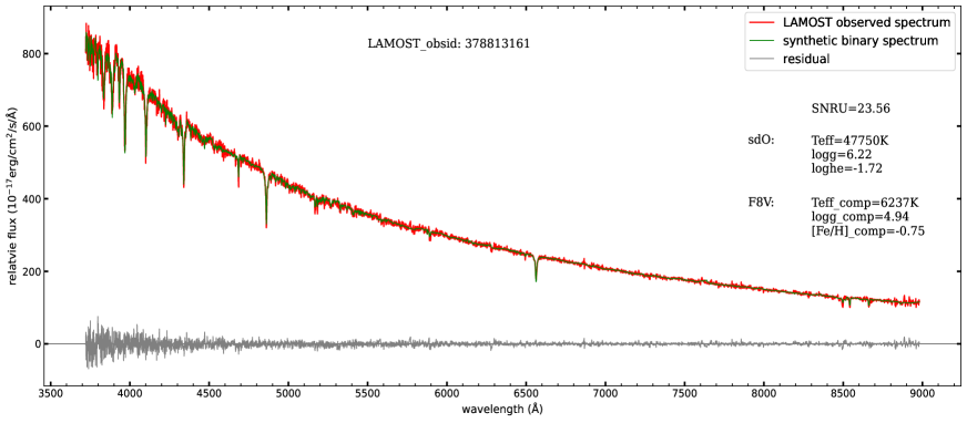
Figure 3: Fitting examples for three composite spectra. Observed spectra are presented by red curves, synthetic binary spectra combined a hot subdwarf spectrum and a cool stellar spectrum are denoted by green curves, while the residuals between observed and synthetic spectra are shown by gray curves. The signal-to-noise ratio in u band (SNRU) of the observed spectra and the atmospheric parameters for the best-fitting synthetic binary spectra are also shown on the right side of each panel.

We used the spectral analysis tool, XTgrid (Németh et al., 2012; Nemeth et al., 2014), to analyze both composite and single-lined spectra. The observed hot subdwarf spectra were reproduced by Synspec synthetic spectra (version 49; Lanz & Hubeny 2007) calculated from non-LTE Tlusty model atmospheres (version 204; Hubeny & Lanz 2017). We used the same steepest-descent $\chi^{2}$ minimization method implemented in XTgrid to fit single-lined spectra in previous work, and recommend the readers to see Lei et al. (2018, 2019b, 2020) for detailed descriptions. The analysis of composite spectra is analogous, but we apply a linear combination of a synthetic hot subdwarf spectrum calculated from Tlusty models and a cool companion spectrum interpolated from ATLAS9 spectra (Mészáros et al., 2012; Bohlin et al., 2017) to render theoretical composite spectra. Then, we iteratively modify the stellar parameters of both components and their flux contribution to the composite spectrum to fit an observation. Once the relative changes of all free parameters and the $\chi^{2}$ are below 0.5%, we consider the fit converged. Next, error calculations are performed in one dimension, changing each parameter until the $\chi^{2}$ reaches the corresponding change for 60% confidence.

The spectral modeling of composite spectra is heavily affected by parameter correlations and large systematics, therefore photometric data were collected from the VizieR Photometry Viewer service within 2 arcseconds around the targets and the spectral energy distribution (SED) was built from these data. The SED was used to optimize the flux contributions of the binary members to the composite continuum.

Fig 3 gives fitting examples for three composite spectra. In the top panel, the observed spectrum (LAMOST_obsid=230104216, red curve) was decomposed to an sdB type spectrum and an F7V type cool spectrum (green curve). The middle panel shows how an sdO type spectrum combined with an F8V type spectrum matched the observed spectrum of LAMOST_obsid=378813161. The spectrum of LAMOST_obsid=360303217 was decomposed to a He-sdOB type spectrum and a K3V type spectrum in the bottom panel. The parameters of the synthetic spectra for the hot and cool components are presented on the right side of each panel.

4 results

By employing the method described in Section 3, 222 hot subdwarf stars were identified, among which 131 stars were identified with composite spectra (see Table 1), and 91 stars with single-lined spectra (see Table 2). We cross-matched our samples with the hot subdwarf catalog of Geier (2020) and found 148 common objects. However, among the 148 common stars, there are 109 objects without atmospheric parameters in the catalog of Geier (2020). It means that our study not only presents 74 new discoveries, but also provides atmospheric parameters for 109 hot subdwarfs that were previously identified but not yet analyzed with atmosphere models.

4.1 Main property table for the samples

Table 1: 131 hot subdwarf stars identified with composite spectra.

	Composite system							Hot primary					Cool secondary
RA	DEC	obs_id	SNRU	source_id	parallax	RUWE	AEN	$G$	$T_{\mathrm{eff}}$	$\mathrm{log}\ g$	$\mathrm{log}(n\mathrm{He}/n\mathrm{H})$	spclass	$T_{\mathrm{eff}}$	$\mathrm{log}\ g$	$\mathrm{[Fe/H]}$	spclass
LAMOST	LAMOST	LAMOST	LAMOST	Gaia	Gaia	Gaia	Gaia(mas)	Gaia(mag)	(K)	(cm  s-2)			(K)	(cm  s-2)
1.025383	23.03016	385811215	25	2848140084112307968	0.4737	1.155	0.145	14.87	36680$\pm$970	6.13$\pm$0.11	-3.75$\pm$0.67	sdB	5997	4.50	-1.00	F5V
4.129504	31.96126	679405182	61	2863196315306344832	0.6322	1.151	0.164	15.37	29930$\pm$860	5.60$\pm$0.06	-1.41$\pm$0.11	sdB	6918	4.89	-0.77	K1V
4.8358078	46.551897	282604062	69	392046852459641472	0.4802	1.487	0.21	14.25	27300$\pm$430	5.35$\pm$0.06	-2.73$\pm$0.53	sdB	6998	5.00	-0.25	F2V
5.7646∗ †	24.3192361	163101192	28	2801217974425183104	0.442	1.249	0.193	15.44	35500$\pm$540	5.98$\pm$0.17	-1.43$\pm$0.07	sdOB	4954	4.91	-0.79	K2V
6.473608∗ †	30.08673	360303217	52	2859002017748155776	0.7413	1.087	0.092	15.06	36860$\pm$160	5.75$\pm$0.06	-0.84$\pm$0.04	He-sdOB	4931	4.85	-1.07	K3V
8.101786	39.183097	697009110	22	380626225180762624	1.2321	9.657	4.814	16.06	30020$\pm$620	5.57$\pm$0.03	-2.21$\pm$0.02	sdB	7244	5.00	-0.65	F0V
10.525503∗ †	5.156504	250216131	62	2554377961881706240	1.091	3.027	0.669	12.78	29720$\pm$180	5.56$\pm$0.20	-3.10$\pm$0.01	sdB	5248	4.98	-0.10	K0V
11.997777∗	3.629061	250209201	21	2550973079312403712	1.7178	1.322	0.206	12.35	44470$\pm$720	6.47$\pm$0.04	-1.97$\pm$0.02	sdO	6471	4.95	-0.51	F7V
12.8622568∗	9.3591384	685611057	30	2581810261598516096	0.797	1.014	0.058	14.18	32860$\pm$160	5.85$\pm$0.22	-2.29$\pm$0.03	sdOB	6251	4.60	-1.00	F5V
13.701168∗ †	6.090181	588011177	30	2553323049193849856	0.4132	1.21	0.255	16.03	27600$\pm$500	5.50$\pm$0.20	-3.04$\pm$0.04	sdB	4753	4.07	-1.87	K3V
16.7959409	51.1731233	248403037	26	404392370879544576	3.2414	4.589	0.759	12.08	35720$\pm$300	5.66$\pm$0.05	-1.32$\pm$0.09	sdOB	5984	4.26	-0.77	F9.5VI
18.3119735∗ †	26.4586702	256010167	70	306837892464925696	1.1299	1.457	0.235	12.84	26910$\pm$50	5.56$\pm$0.13	-2.23$\pm$0.30	sdB	6295	4.96	-0.69	F8V
20.438896	26.94654	281001143	37	296407654581453824	0.5291	1.184	0.113	14.61	26390$\pm$140	5.53$\pm$0.04	-2.01$\pm$0.03	sdB	5997	3.50	-0.75	G0IV
26.809005	2.629267	384203051	26	2512318137425806720	0.521	1.005	0.064	15.62	34700$\pm$330	6.01$\pm$0.14	-1.51$\pm$0.14	sdOB	6397	4.80	-0.67	F7V
41.060213∗ †	30.123075	108311209	11	129720592299213056	0.5517	1.187	0.125	14.55	32750$\pm$1060	5.79$\pm$0.18	-1.67$\pm$0.13	sdB	6982	5.00	-0.95	F2.5V
49.08386∗ †	0.706325	633209035	15	3266182479530739328	0.6927	1.045	0.081	15.10	32260$\pm$170	5.65$\pm$0.06	-4.26$\pm$0.58	sdB	6456	4.92	-0.75	F7V
49.1125671∗ †	14.5351142	593905069	11	30166132300899584	0.5398	0.998	0.0	15.80	46050$\pm$3560	6.68$\pm$0.11	-1.88$\pm$0.17	sdO	5997	4.61	-0.69	G1V
53.069742∗ †	-2.550527	307910106	36	3261350091567233920	1.019	1.291	0.13	12.56	34290$\pm$250	5.52$\pm$0.28	-1.94$\pm$0.01	sdB	6918	4.34	-0.08	F0V
58.278732	16.813495	280504020	35	43520323793261440	-0.503	14.706	4.874	14.71	25520$\pm$110	5.72$\pm$0.07	-3.44$\pm$0.16	sdB	4497	5.00	-0.01	F3IV
58.3071641∗ †	25.7560623	758711067	328	67303928533459968	2.3552	2.715	0.37	10.12	40410$\pm$540	5.31$\pm$0.08	1.06$\pm$0.10	He-sdOB	5495	2.00	-1.00	F6IV/V
60.279188∗ †	15.596102	280506023	45	40154478181532544	0.9774	0.97	0.0	14.26	38170$\pm$520	6.03$\pm$0.02	-1.12$\pm$0.03	sdOB	6714	4.92	-0.48	F5V
60.8944383∗ †	26.0665106	264511018	46	162510331145182976	2.2913	2.039	0.282	12.27	31680$\pm$530	6.11$\pm$0.06	-5.67$\pm$0.28	sdB	6456	4.91	-0.25	F7V
66.6441208∗ †	16.9241472	420209010	20	3313745222245617664	1.1816	1.597	0.145	13.79	33290$\pm$1550	5.87$\pm$0.29	-3.59$\pm$0.71	sdB	6918	5.00	-0.33	K1V
74.997049∗ †	16.406036	402712100	11	3405336220170607360	0.5485	1.034	0.0	15.87	31900$\pm$170	6.70$\pm$0.04	-1.81$\pm$0.07	sdOB	6501	4.85	-0.93	F6V
75.79921	42.25386	363101011	16	201795194412994432	1.1	0.946	0.135	14.31	30700$\pm$890	5.24$\pm$0.08	-2.23$\pm$0.08	sdB	3749	5.00	-2.50	M2V
80.535505	39.628034	252808221	24	187949697318585856	0.9701	0.983	0.131	15.19	39110$\pm$660	5.71$\pm$0.10	-1.02$\pm$0.04	sdOB	7261	4.99	0.52	F0V
103.2504	34.471604	189108156	27	939393979967463424	0.453	1.177	0.198	15.58	34540$\pm$460	5.81$\pm$0.07	-3.31$\pm$0.36	sdB	7227	5.00	-1.46	F0V
103.3741167	25.2871169	686711052	31	3381734176584838528	0.7634	1.039	0.164	12.78	28400$\pm$440	6.66$\pm$0.04	-2.45$\pm$0.01	sdB	7780	4.88	-0.22	A8V
106.11298	36.912729	336403222	35	946065369848575872	0.6036	1.535	0.34	15.37	29640$\pm$450	5.69$\pm$0.03	-2.92$\pm$0.14	sdB	4064	4.63	-1.25	K7V
108.903728	0.351749	778603202	13	3111129624664152064	1.1696	3.57	1.287	16.29	28080$\pm$110	5.21$\pm$0.08	-2.66$\pm$0.19	sdB	4753	5.00	-1.06	K3V
109.54489	9.9644258	446310079	11	3156485441381866368	0.6282	5.439	1.04	14.75	29400$\pm$3840	6.92$\pm$1.44	-0.62$\pm$1.37	He-sdOB	8035	5.00	-0.47	A8V
109.89297	11.856675	386307217	40	3163010252616980608	0.718	1.763	0.29	14.31	61800$\pm$650	5.25$\pm$0.36	-1.41$\pm$0.08	sdO	5942	5.00	-0.59	G1V
112.2235416∗ †	53.7169814	425914149	24	983992164455024512	0.7676	1.045	0.068	13.92	34550$\pm$710	5.88$\pm$0.13	-1.47$\pm$0.07	sdOB	6237	3.94	-1.12	F3V
112.8519	37.216993	184404173	27	898706032489528064	0.2873	1.039	0.031	15.36	32170$\pm$1220	5.48$\pm$0.12	-4.59$\pm$1.26	sdB	6760	5.00	-0.23	F5V
114.30113∗ †	26.706866	3407169	11	872072016870129024	0.6281	1.219	0.168	15.07	30200$\pm$330	5.78$\pm$0.08	-4.38$\pm$0.02	sdB	5997	5.00	-1.25	G0V
114.46526	17.03408	417216043	35	3169072650493941248	0.8258	1.436	0.209	14.17	37980$\pm$700	5.89$\pm$0.05	-1.39$\pm$0.47	sdOB	6471	5.00	-0.21	F7V
115.34127∗ †	26.907168	183710065	36	869167966142655616	0.4764	1.062	0.131	15.57	33750$\pm$420	5.47$\pm$0.05	-3.11$\pm$0.66	sdB	6760	5.00	-0.98	F5V
115.80866∗ †	40.564067	334308156	20	923503803562868608	0.5006	1.079	0.098	15.11	33550$\pm$1010	5.01$\pm$0.10	-2.65$\pm$0.13	sdB	7161	5.00	-0.58	F0V
120.74917∗	41.243885	279212200	24	921531554580422016	0.5674	1.005	0.193	15.25	44880$\pm$540	5.08$\pm$0.13	2.42$\pm$0.47	He-sdOB	6266	4.89	0.75	F8V
123.52831∗ †	20.317123	268114178	13	675664193216392704	0.3463	1.052	0.104	15.74	26480$\pm$180	5.23$\pm$0.21	-1.95$\pm$0.04	sdOB	6516	5.00	-0.73	F6V
125.0139583∗ †	17.6539556	698903042	38	656345533398638464	0.408	0.998	0.0	15.09	39240$\pm$860	5.60$\pm$0.03	-1.59$\pm$0.04	sdOB	7112	4.71	-0.39	F2V
126.14188∗ †	30.481857	287014148	14	708829002962898304	0.2979	1.02	0.067	15.20	49440$\pm$3260	6.09$\pm$0.22	-1.48$\pm$0.02	sdO	6516	3.65	-0.73	F5V
126.279986∗ †	20.110442	602205226	34	663802902294594944	0.5254	1.008	0.06	14.84	34040$\pm$490	6.27$\pm$0.05	-1.47$\pm$0.12	sdOB	6501	4.97	-0.50	F6V
126.324962∗ †	11.518417	19506063	13	601188910547673728	0.6931	1.032	0.077	14.63	32480$\pm$500	5.88$\pm$0.05	-1.27$\pm$0.04	sdB	6223	4.52	-0.79	F8V
127.26092∗ †	22.776878	321902192	24	677934238056557312	0.4904	1.028	0.071	15.80	38730$\pm$460	6.27$\pm$0.06	-1.47$\pm$0.13	sdOB	6081	4.62	-0.74	G0V
130.5431333∗ †	-2.2211	309414071	28	3072364177559581696	0.8832	1.017	0.125	12.98	28860$\pm$940	6.26$\pm$0.03	-3.96$\pm$0.24	sdB	7413	5.00	-0.34	F0V
130.662525	3.019274	313902052	78	3079278864452011904	1.7164	1.155	0.158	12.24	35970$\pm$910	6.58$\pm$0.09	-1.29$\pm$0.20	sdOB	6456	4.95	-0.05	F6V
130.8190788	25.0614547	779313103	19	690626278727938560	1.023	1.013	0.0	13.44	30830$\pm$480	5.70$\pm$0.13	-2.63$\pm$0.17	sdB	6137	4.77	-0.36	G0V
134.858699∗ †	7.987002	503806026	20	585028765383068288	0.3241	0.965	0.0	16.29	35080$\pm$310	5.68$\pm$0.04	-1.58$\pm$0.03	sdOB	6109	5.00	-0.89	G0V
139.12066∗ †	24.653384	187512028	12	687691269876173056	0.4114	1.083	0.106	15.35	27680$\pm$610	5.11$\pm$0.05	-2.53$\pm$0.09	sdB	6531	4.84	-0.48	F7V
150.19358∗ †	2.9024758	316603031	14	3836440886741718784	0.2373	1.058	0.101	16.36	37420$\pm$1700	5.72$\pm$0.04	-1.25$\pm$0.15	sdOB	6501	4.47	-0.50	F7V
150.80983∗ †	21.856699	139801107	16	629594278053946752	0.2882	1.0	0.085	15.95	36920$\pm$3700	6.59$\pm$0.45	-1.43$\pm$0.21	sdOB	6501	5.00	-0.50	F6V
150.83197∗ †	37.276345	400914083	42	802020653597763584	0.7726	1.099	0.131	14.92	28180$\pm$30	5.85$\pm$0.07	-1.53$\pm$0.08	sdOB	4731	3.46	-0.77	K3V
154.48904∗ †	35.921533	400906249	23	753807962069995648	0.323	2.136	0.66	15.99	35170$\pm$450	6.03$\pm$0.03	-1.39$\pm$0.23	sdOB	6251	4.89	-0.70	F8V
155.63489∗ †	34.415639	545115199	27	752309185986742912	0.1894	1.056	0.0	16.08	38080$\pm$400	5.72$\pm$0.20	-1.59$\pm$0.08	sdOB	6251	3.36	-0.75	F6III
164.771809∗ †	32.105757	200313100	38	736957808935190656	0.4385	1.16	0.137	14.63	32370$\pm$510	5.17$\pm$0.03	-2.25$\pm$0.32	sdB	6966	5.00	-0.55	F2.5V
165.54621∗ †	26.279526	389604033	27	3996780498461572480	0.3261	1.04	0.061	15.06	31100$\pm$120	6.78$\pm$0.07	-1.87$\pm$0.08	sdB	6338	4.66	-0.74	A0V
166.859281∗	24.053095	385107015	165	3995351343799453056	3.4105	2.301	0.478	11.20	32310$\pm$180	6.25$\pm$0.02	-1.77$\pm$0.02	sdOB	5997	3.99	-0.75	G0V
168.322177∗ †	4.220697	619310054	76	3812248366755810944	0.9561	1.156	0.168	14.73	33090$\pm$50	5.86$\pm$0.01	-1.73$\pm$0.07	sdOB	4246	5.00	-0.59	K7V
170.55461∗ †	14.439381	120710031	18	3966770015776476928	0.2078	1.047	0.181	16.11	34100$\pm$300	5.67$\pm$0.02	-3.66$\pm$0.03	sdB	6237	4.47	-1.25	F3V
172.809697∗ †	9.5386	103506220	23	3914518169503182848	1.0965	1.681	0.293	14.36	35050$\pm$540	5.96$\pm$0.02	-1.71$\pm$0.05	sdOB	5432	3.75	-1.69	G8V
174.2646708∗ †	14.8445056	291306190	12	3972199752086976000	0.0895	3.442	1.275	16.58	31680$\pm$860	5.81$\pm$0.09	-1.43$\pm$0.16	sdOB	6776	5.00	-1.02	F5V
180.8311583∗ †	9.1643472	815013177	11	3906031520285024512	0.5757	1.213	0.148	14.61	37420$\pm$1070	6.18$\pm$0.16	-1.13$\pm$0.04	sdOB	6165	4.91	-1.04	F8V
183.1606958∗ †	42.6672917	149310130	17	1536809808987373824	0.5874	0.987	0.034	14.89	38060$\pm$190	5.70$\pm$0.06	-1.24$\pm$0.09	sdB	6338	4.67	-0.75	A0V
183.2190457∗ †	33.9006855	433107100	71	4028634144887638016	1.2878	1.129	0.128	12.62	40600$\pm$190	5.76$\pm$0.06	-1.32$\pm$0.01	sdOB	6516	4.95	-0.46	F6V
184.399697∗ †	37.973573	497901202	27	1532409357294653824	0.3042	1.125	0.172	15.52	27800$\pm$610	5.45$\pm$0.09	-2.56$\pm$0.07	sdB	5997	3.03	-0.78	G0III
188.2903208∗ †	8.576175	220701149	26	3902809057861940480	0.463	0.901	0.0	15.49	36730$\pm$1280	6.14$\pm$0.06	-1.01$\pm$0.07	sdOB	5754	3.50	-0.48	F3V
188.712025∗ †	49.789125	448512117	34	1544410045677548288	0.9806	2.009	0.349	13.91	32000$\pm$1160	5.71$\pm$0.11	-2.53$\pm$0.04	sdB	6966	4.54	-0.69	F2V
192.518425∗ †	55.100589	152807229	48	1570548009752602240	4.0109	0.721	0.432	12.67	32160$\pm$230	6.06$\pm$0.07	-0.91$\pm$0.48	sdOB	4753	5.00	-0.18	K3V
192.75618∗ †	37.180479	336710181	22	1517524890432603520	0.3881	1.067	0.1	15.53	50640$\pm$2860	6.04$\pm$0.09	-1.54$\pm$0.03	sdO	6382	4.75	-0.88	F4V
194.0204403	28.1221093	459203172	26	1463780590268542592			4.673	13.24	29450$\pm$1720	5.46$\pm$0.09	-2.88$\pm$0.12	sdB	6067	3.14	-0.46	G0III
195.0576423∗ †	-2.831275	105604229	14	3685172413454924544	0.7025	1.019	0.054	13.96	30130$\pm$1410	5.13$\pm$0.07	-2.38$\pm$0.08	sdB	6237	3.48	-0.74	F8V
198.387516∗ †	36.946957	563102088	10	1474359575755115136	0.9446	1.113	0.292	14.53	26970$\pm$1540	5.51$\pm$0.07	-3.08$\pm$0.88	sdB	5997	5.00	0.50	G0V?
199.1605083∗ †	3.8050667	645310072	15	3715866036458578688	0.8111	3.738	1.628	16.14	33470$\pm$510	5.65$\pm$0.04	-1.58$\pm$0.13	sdOB	4753	5.00	-1.50	K3V
199.9733469	12.0661869	414507200	134	3739487119636315520	1.7705	1.849	0.458	11.26	41890$\pm$520	5.18$\pm$0.02	-2.13$\pm$0.05	sdO	6745	4.98	-0.43	F5V
201.313488∗ †	38.883599	563108029	28	1476298186553761664	0.3035	1.069	0.124	16.22	37260$\pm$430	6.06$\pm$0.14	-1.70$\pm$0.15	sdOB	5701	4.90	-1.00	G3V
207.73692∗ †	8.019409	451307046	13	3721767012285435520	0.3076	1.004	0.0	15.76	33220$\pm$2640	5.30$\pm$0.19	-2.19$\pm$0.15	sdB	6683	4.50	-0.75	F5V
210.0127583∗ †	23.7499944	316208195	21	1256917132588516224	0.2031	2.808	0.656	15.14	44350$\pm$1480	5.75$\pm$0.58	0.27$\pm$0.15	He-sdOB	5199	4.55	-2.25	G8V
210.3218∗ †	27.6451083	332010163	16	1450983271353426048	0.2796	1.003	0.0	15.99	37780$\pm$1160	6.01$\pm$0.09	-1.08$\pm$0.08	sdOB	7063	5.00	-0.94	F2V
210.6369292∗ †	32.2559694	230104216	11	1454622105085650688	0.4233	0.981	0.0	14.97	35150$\pm$210	5.64$\pm$0.03	-4.01$\pm$0.25	sdB	6412	4.82	-0.75	F7V
210.821918∗ †	22.172126	573612151	29	1256509935329189120			16.67	15.91	35340$\pm$870	5.67$\pm$0.14	-1.01$\pm$0.02	sdOB	6011	5.00	-1.23	G0V
212.317154∗ †	38.475605	242115019	27	1485199008058786688	0.4356	1.027	0.069	16.04	43170$\pm$370	6.00$\pm$0.12	-1.48$\pm$0.18	sdO	5997	5.00	-0.75	G0V
215.27003∗ †	17.608	425408223	20	1232778626111037184	0.3108	1.079	0.157	16.27	33870$\pm$120	5.78$\pm$0.02	-1.38$\pm$0.09	sdOB	5997	4.99	-1.04	G0V
215.8780875∗ †	14.8089694	302514109	15	1228629618983512064	0.2106	0.987	0.117	15.26	34520$\pm$100	5.14$\pm$0.08	-1.93$\pm$0.27	sdB	6745	5.00	-1.21	F5V
215.8983417∗ †	34.2387222	438302106	46	1479772643298162176	0.6344	1.017	0.0	14.70	40060$\pm$1800	6.39$\pm$0.29	-1.43$\pm$0.02	sdOB	6251	5.00	-0.25	G0V
222.0906375∗ †	31.5184417	660103039	23	1283389867897035392	0.2348	1.03	0.0	16.24	38820$\pm$40	5.09$\pm$0.91	-1.39$\pm$0.09	sdOB	6501	4.97	-0.49	F6V
227.77946∗ †	17.537572	581401069	17	1211503282272546432	0.4243	0.999	0.0	16.15	32270$\pm$880	5.67$\pm$0.11	-2.60$\pm$0.10	sdB	6441	4.39	-0.67	F6V
229.055053∗	27.648553	558307059	23	1271587607005565440	0.1436	1.037	0.211	16.48	53820$\pm$1770	5.70$\pm$0.18	-1.58$\pm$0.19	sdO	5834	4.68	-1.66	F8V
229.3097958∗ †	3.1742833	723007009	18	4421940758497428096	0.8424	1.343	0.187	13.91	32190$\pm$100	5.85$\pm$0.03	-1.73$\pm$0.02	sdOB	5984	4.63	-0.83	G1V
229.535314∗	4.178841	237508148	14	1155791990165521920	0.5414	1.125	0.18	15.31	37620$\pm$110	6.13$\pm$0.32	-1.79$\pm$0.05	sdOB	5956	3.97	-1.22	G1V
230.611347∗ †	24.726743	581904203	12	1270016817203702400	0.3453	0.981	0.0	15.60	30920$\pm$700	5.45$\pm$0.09	-2.24$\pm$0.12	sdB	6652	4.53	-0.34	F5V
231.01266∗ †	1.572694	431411183	19	4420741294390728448	0.9773	1.564	0.215	13.87	23720$\pm$690	5.28$\pm$0.07	-3.15$\pm$0.14	sdB	5069	5.00	0.32	K1V
231.4727042∗ †	43.6909778	745010247	25	1394116942282089344	0.7262	1.187	0.176	15.05	36850$\pm$100	5.75$\pm$0.16	-0.51$\pm$0.01	He-sdOB	5000	5.00	0.00	K2V
233.013331∗ †	42.962491	573411193	21	1391344214475144832	0.5505	1.142	0.164	15.23	35800$\pm$2590	6.29$\pm$0.33	-1.34$\pm$0.42	sdOB	6683	4.86	-0.71	F5V
234.530673∗ †	27.6954506	221010099	10	1224346643237436288	0.7733	1.019	0.013	13.72	40460$\pm$4510	5.12$\pm$0.54	-1.30$\pm$0.09	sdOB	6561	4.62	-0.44	F6V
238.3402865∗ †	25.4037151	662002168	17	1220195948186053760	1.5392	2.778	0.53	14.19	23550$\pm$450	5.68$\pm$0.03	-4.06$\pm$0.60	sdB	4753	5.00	-0.50	K3V
240.486021	6.314934	568315063	37	4450708930484104960	0.7211	1.404	0.207	14.82	27250$\pm$20	5.45$\pm$0.13	-2.63$\pm$0.06	sdB	5188	5.00	-0.56	K0V
240.537772∗	7.419737	568316229	32	4451111935856224000	0.7051	0.976	0.093	14.46	73400$\pm$19720	5.96$\pm$0.13	-1.74$\pm$0.18	sdO	5847	5.00	-0.41	G2V
241.54936∗ †	3.8714259	744001168	25	4413410266254905344	0.3737	0.986	0.0	15.48	34510$\pm$560	5.96$\pm$0.07	-1.23$\pm$0.12	sdOB	6918	4.84	-0.61	F2V
243.1328155∗ †	57.2476258	812903110	11	1621996774452667648	0.1664	0.976	0.0	17.48	33720$\pm$1890	5.58$\pm$0.12	-6.66$\pm$0.01	sdB	6295	4.60	-0.99	A0V
244.526825∗ †	21.6903639	461106067	25	1202447086032118784	0.6055	1.046	0.073	14.80	31960$\pm$420	6.71$\pm$0.17	-1.55$\pm$0.05	sdOB	6237	5.00	-1.01	F8V
252.59188∗ †	31.463808	347313144	12	1313140659676082560	0.5871	1.144	0.184	15.82	37680$\pm$390	6.10$\pm$0.04	-0.19$\pm$0.03	He-sdOB	4742	4.48	-0.39	K3V
252.791963∗ †	8.059091	331602037	23	4442343330624541568	0.6845	1.262	0.1	13.71	40490$\pm$210	5.80$\pm$0.11	-1.20$\pm$0.19	sdOB	6194	4.87	-0.31	F8V
254.674322∗	41.521005	566911146	25	1354579844177083904	0.4121	0.933	0.0	15.99	33360$\pm$410	5.67$\pm$0.05	-1.92$\pm$0.05	sdOB	5861	4.21	-1.14	G1.5V
258.9182625∗ †	34.3821528	576806137	10	1334991769651067904	0.362	1.081	0.115	15.49	29940$\pm$300	5.45$\pm$0.11	-1.79$\pm$0.08	sdB	6501	5.00	-0.75	F6V
259.938993	51.869609	580916012	22	1415898405068162176			8.596	13.80	32290$\pm$850	5.37$\pm$0.16	-3.66$\pm$0.29	sdB	6095	5.00	-0.66	G0V
261.6163772∗ †	37.155398	141504052	13	1337240374008902784	0.9327	1.19	0.086	13.31	41310$\pm$960	6.26$\pm$0.15	-1.86$\pm$0.17	sdO	6934	4.85	-0.50	F2V
261.9515653∗	16.7492625	342803178	62	4550114402362108416	1.1289	2.847	0.524	13.48	27550$\pm$90	5.43$\pm$0.01	-3.17$\pm$0.20	sdB	4497	5.00	-0.86	K7V
268.5154∗ †	53.6932417	155403168	14	1369049829516110336	0.5823	1.036	0.035	15.26	48160$\pm$8070	5.26$\pm$0.16	-1.62$\pm$0.18	sdO	6237	5.00	0.05	G0V
272.61257	14.261412	746402012	25	4497397527098931712	0.4661	1.05	0.21	16.29	25790$\pm$210	5.80$\pm$0.04	-2.44$\pm$0.01	sdB	4753	4.45	-0.23	K2V
273.35417	6.8877511	742403249	22	4478006677464647040	0.5729	1.379	0.36	15.95	46110$\pm$1850	5.14$\pm$0.20	0.76$\pm$1.05	He-sdOB	4753	5.00	0.50	K3V
278.15735	11.778036	746709096	10	4481070569714541056	0.4538	0.978	0.0	17.19	36290$\pm$720	5.72$\pm$0.09	-1.49$\pm$0.23	sdB	6652	4.81	-0.50	F5V
284.946255∗ †	57.6758294	346813058	19	2153548180479601280	0.3662	1.001	0.064	14.81	40410$\pm$1080	5.88$\pm$0.16	-2.74$\pm$0.13	sdO	6745	4.97	-0.75	F5V
287.5008566∗ †	46.6734565	354401198	35	2130430570550718464	0.498	1.007	0.065	14.47	44360$\pm$5230	5.76$\pm$0.20	-1.84$\pm$0.47	sdO	6251	4.57	-1.01	F5V
289.0894514	48.4702516	353802136	60	2132462777275978624	0.5795	1.002	0.07	14.39	30460$\pm$700	5.56$\pm$0.21	-2.38$\pm$0.05	sdB	6714	4.80	-0.79	F5V
290.0299828	52.0936831	353811024	56	2139296001523913728	0.726	0.986	0.0	14.39	33890$\pm$100	6.22$\pm$0.07	-1.65$\pm$0.03	sdOB	6471	4.82	-0.69	F7V
305.11349∗	7.0704421	587205114	60	4249848840652401792	0.869	1.325	0.164	14.10	74200$\pm$1810	5.44$\pm$0.08	2.34$\pm$0.19	He-sdO	6966	5.00	-0.42	F2.5V
319.4259042∗ †	-0.1055306	677910180	30	2689440797710883584	0.3705	1.087	0.086	15.02	36630$\pm$1640	5.83$\pm$0.13	-1.20$\pm$0.06	sdOB	6382	4.77	-0.75	F7V
320.259476∗ †	12.847195	260814117	18	1746937544892092416	0.7124	1.265	0.121	13.49	48560$\pm$1710	5.60$\pm$0.21	-2.63$\pm$0.12	sdO	6295	4.10	0.03	F8V
320.6041	17.862396	593101087	43	1785228484006179456	0.6792	1.112	0.082	14.33	56750$\pm$3940	6.46$\pm$0.08	-1.31$\pm$0.14	sdO	6501	5.00	-0.54	F6V
321.10134∗	15.105552	685407021	87	1783474797319468032	1.5707	1.502	0.248	12.95	39090$\pm$170	5.69$\pm$0.02	-1.17$\pm$0.20	sdOB	6531	4.95	-0.46	F6V
321.22878∗	15.984361	592411060	54	1783691847786812288	0.8228	1.575	0.244	14.40	29930$\pm$60	6.30$\pm$0.77	-2.04$\pm$0.39	sdB	6165	4.46	-0.98	F5V
321.743738∗ †	7.34571	372505162	32	1739298997095482240	0.9628	1.161	0.097	14.03	36680$\pm$70	6.19$\pm$0.01	-1.64$\pm$0.17	sdOB	6251	4.95	-0.73	F8V
321.870759	31.3114233	368209056	49	1853416896629422464	0.9232	2.126	0.36	14.43	27760$\pm$70	5.26$\pm$0.04	-2.62$\pm$0.04	sdB	4092	4.69	-1.25	K7V
322.275089∗ †	0.75258	677909003	47	2688012605121741312	0.2962	1.027	0.115	15.50	37230$\pm$440	5.76$\pm$0.03	-1.24$\pm$0.18	sdOB	4753	4.50	-0.75	K2V
332.161998	14.819503	378813161	24	1774431039302375552	0.3556	1.041	0.091	15.79	47750$\pm$830	6.22$\pm$0.04	-1.72$\pm$0.03	sdO	6237	4.94	-0.75	F8V
334.627458∗	18.802447	75311209	13	1777173805417611776	1.1962	2.117	0.291	13.84	31910$\pm$370	5.83$\pm$0.05	-1.74$\pm$0.04	sdOB	4508	5.00	-1.49	K4V
343.32667∗ †	21.898433	490613065	26	2835948493025229952	0.8726	0.967	0.008	13.06	34510$\pm$230	5.39$\pm$0.08	-2.56$\pm$0.26	sdB	6698	4.40	-0.30	F5V
350.122232∗ †	28.494027	249901087	52	2845145731696691968	1.3136	0.956	0.101	11.87	26200$\pm$480	6.11$\pm$1.25	-1.93$\pm$0.52	sdOB	6714	4.42	-0.29	F5IV
352.02525∗ †	50.621368	689003056	19	1943261255910215552	0.2068	1.131	0.212	16.70	33640$\pm$640	5.74$\pm$0.07	-6.99$\pm$0.09	sdB	6745	5.00	-0.50	F5V
354.63865∗ †	47.495592	678715215	30	1940032157758205824	-0.0189	1.082	0.148	16.24	26600$\pm$230	6.58$\pm$0.13	-5.14$\pm$0.17	sdB	7533	4.71	-0.32	A8V

Table 1 gives the main properties of 131 hot subdwarf stars identified with composite spectra. From columns (1) to (4), the table presents right ascension (RA), declination (DEC), LAMOST_obsid and signal to noise ratio in LAMOST u band (SNRU), respectively. Columns (5) to (9) give the source_id, parallaxes, RUWE values, astrometric excess noise (AEN) and magnitudes in the G band of Gaia EDR3. Columns (10) to (13) give effective temperatures ($T_{\rm eff}$), gravity ($\log{g}$), helium abundance ($\log(n{\rm He}/n{\rm H})$) and spectral classification for the hot subdwarf primary. While columns (14) to (17) give the effective temperatures, gravity, metallicity ([Fe/H]) and spectral classification for the companion stars based on the fitting results.

In Table 2, the main properties of 91 hot subdwarf stars identified with single-lined spectra were presented. Columns (1) to (4) give the right ascension (RA), declination (DEC), LAMOST_obsid and SNRU, respectively. Columns (5) to (6) give the source_id, and magnitudes in G band of Gaia EDR3, while columns (7) to (10) give the detailed atmospheric parameters (i.e., $T_{\rm eff}$, $\log{g}$, $\log(n{\rm He}/n{\rm H})$ and their uncertainties) and spectral classification. Objects with RA labeled by ^∗ both in Table 1 and 2 are common stars in the catalog of Geier (2020) and also have reported atmospheric parameters, while objects with RA labeled by ^∗ and ^† are common stars in the catalog of Geier (2020) but without atmospheric parameters there.

Table 2: 91 hot subdwarf stars identified by single-lined spectra.

RA	DEC	obs_id	SNRU	source_id	$G$	$T_{\mathrm{eff}}$	$\mathrm{log}\ g$	$\mathrm{log}(n\mathrm{He}/n\mathrm{H})$	spclass
LAMOST	LAMOST	LAMOST	LAMOST	Gaia	Gaia(mag)	(K)	(cm  s-2)
7.4749346	50.541949	594011103	30	391755859836391680	16.18	29210$\pm$560	5.49$\pm$0.13	-2.92$\pm$0.37	sdB
17.2632275∗ †	52.7300771	248315093	20	404959035980962944	15.49	32250$\pm$460	5.41$\pm$0.04	-2.60$\pm$0.10	sdB
29.0050281	40.0561321	264312040	122	344155939885410816	11.43	28380$\pm$330	5.31$\pm$0.03	-2.62$\pm$0.04	sdB
32.881148∗ †	39.287209	613410220	31	332606704106366848	15.54	35370$\pm$990	5.94$\pm$0.10	-1.64$\pm$0.03	sdOB
33.933972∗ †	33.668954	601516009	108	326009496898928896	13.72	27990$\pm$190	5.44$\pm$0.02	-2.81$\pm$0.03	sdB
36.524742	55.982399	678103210	35	457462812156715008	16.06	37640$\pm$460	5.39$\pm$0.07	-3.25$\pm$0.40	sdB
37.082246	36.948326	778503239	15	328366815470365952	16.84	28180$\pm$280	5.26$\pm$0.04	-1.95$\pm$0.02	sdB
37.34398	55.681828	678104014	13	457250400255056768	17.12	28040$\pm$220	5.22$\pm$0.09	-2.91$\pm$0.04	sdB
45.366714	30.260161	198207185	29	123108816565129344	14.97	60550$\pm$4720	6.02$\pm$0.12	-2.25$\pm$0.16	sdO
46.533112∗	38.393252	473710095	11	142548697540212352	16.80	36800$\pm$1990	6.11$\pm$0.20	-1.93$\pm$0.11	sdOB
49.405835∗	37.486865	255501173	37	235323736345986176	15.30	28980$\pm$220	5.48$\pm$0.02	-2.90$\pm$0.02	sdB
54.679217	30.388769	188007106	15	120354952254440960	16.57	32920$\pm$540	5.58$\pm$0.09	-1.48$\pm$0.05	sdB
57.507775∗	32.74251	301301092	11	217062978512976000	17.24	31530$\pm$250	5.97$\pm$0.54	-2.19$\pm$0.04	sdB
61.6862792	22.7204186	796803063	33	53566385439973376	14.37	28980$\pm$170	5.55$\pm$0.02	-2.99$\pm$0.06	sdB
65.145303∗	1.3446668	777816028	84	3255780171819962496	12.30	44790$\pm$320	5.33$\pm$0.07	1.91$\pm$0.35	He-sdOB
73.813501∗	13.091574	402801174	13	3296244226946647168	17.15	29420$\pm$610	5.37$\pm$0.09	-2.68$\pm$0.04	sdB
77.99079	23.93592	757003099	21	3418841422712575616	16.72	41070$\pm$520	5.44$\pm$0.01	1.44$\pm$0.04	He-sdOB
80.752383∗ †	18.457499	616504175	23	3400623129219934336	16.56	40200$\pm$670	5.40$\pm$0.06	2.47$\pm$0.03	He-sdB
82.637651∗	11.345517	606308098	15	3340622921426651648	16.71	28850$\pm$340	5.80$\pm$0.16	-2.88$\pm$0.23	sdB
88.065822	43.88204	714502122	13	193503502346470784	16.24	27510$\pm$390	5.52$\pm$0.03	-2.58$\pm$0.09	sdB
88.9259708∗	64.1363	614505205	22	287018271958898560	13.24	53290$\pm$1940	5.49$\pm$0.07	-2.16$\pm$0.15	sdO
110.41193	5.7395204	769308212	14	3140865744837849216	14.86	42220$\pm$620	5.50$\pm$0.05	-0.21$\pm$0.07	He-sdOB
114.9939542∗ †	17.9763889	725308189	23	671353867118310528	14.92	31330$\pm$180	5.46$\pm$0.03	-3.27$\pm$0.12	sdB
115.35463	12.838747	688807112	11	3163891442466252928	17.25	39300$\pm$560	5.64$\pm$0.12	-0.20$\pm$0.09	He-sdOB
118.700879	1.770195	779707047	78	3087687074686316416	14.24	34720$\pm$250	5.91$\pm$0.05	-0.74$\pm$0.04	He-sdOB
120.18431	18.067203	712912143	14	669097841055847296	16.04	29360$\pm$320	5.31$\pm$0.05	-1.56$\pm$0.12	sdB
127.00848∗ †	40.669153	811303149	12	914500864915422848	17.92	43160$\pm$1370	5.58$\pm$0.07	-1.92$\pm$0.49	sdO
131.48705∗ †	13.8700278	792102231	14	609252591386688256	17.43	24530$\pm$270	5.58$\pm$0.14	-3.94$\pm$0.59	sdB
131.5497792∗ †	24.4201722	779213036	12	690346315579638656	15.58	28930$\pm$390	5.48$\pm$0.05	-3.08$\pm$0.03	sdB
133.0738375∗	21.2768861	700706139	10	685761455170072192	16.30	29580$\pm$360	5.58$\pm$0.06	-6.10$\pm$0.60	sdB
135.7208206∗	7.592742	781214052	15	584194373496664064	17.30	42750$\pm$360	6.29$\pm$0.08	1.26$\pm$0.06	He-sdOB
150.1573529	18.2564037	778710002	14	626203208100096896	16.87	28750$\pm$850	5.38$\pm$0.21	-2.50$\pm$0.15	sdB
150.17257∗	36.752124	803414182	13	795998387893409152	16.97	27280$\pm$300	5.47$\pm$0.10	-2.73$\pm$0.07	sdB
153.175889∗	48.82705	613703104	25	822945768622050048	16.45	29910$\pm$1040	5.50$\pm$0.15	-2.44$\pm$0.12	sdB
156.16429∗ †	38.654983	811404140	11	755712414993199744	16.78	30830$\pm$400	5.67$\pm$0.10	-2.16$\pm$0.07	sdB
166.1875917∗	9.4255167	660505073	31	3867259957150344960	16.27	36720$\pm$280	5.20$\pm$0.06	-2.30$\pm$0.09	sdOB
170.261064∗ †	5.816939	619315126	101	3813980166288451072	14.21	29870$\pm$30	5.58$\pm$0.04	-3.07$\pm$0.40	sdB
171.3625∗	11.4839972	779809104	10	3915826137367906816	17.34	34350$\pm$490	6.01$\pm$0.05	-0.96$\pm$0.06	He-sdOB
178.49506∗	35.658008	633010131	35	4031612751951454080	16.47	30110$\pm$270	5.59$\pm$0.05	-3.25$\pm$0.22	sdB
180.96765∗	23.895365	629804097	30	4002664328779500928	16.99	40020$\pm$720	5.75$\pm$0.10	-0.51$\pm$0.08	He-sdOB
190.5072255∗	43.6731474	803515195	22	1540495440685138432	16.92	35540$\pm$670	5.89$\pm$0.10	-0.34$\pm$0.05	He-sdOB
192.6661291∗ †	75.8833605	644104043	29	1692116238728076544	15.36	72360$\pm$3110	5.47$\pm$0.10	0.64$\pm$0.11	He-sdO
193.8111	37.541553	795403228	31	1517595224818622976	15.74	56060$\pm$1490	7.20$\pm$0.08	-2.10$\pm$0.26	sdO
196.3399572	38.9833266	795409037	24	1523599314219554432	16.79	40770$\pm$540	6.52$\pm$0.15	-2.29$\pm$0.05	sdO
201.9527625∗	9.9139972	783505160	68	3732055520543728256	13.94	34640$\pm$650	5.83$\pm$0.04	-1.82$\pm$0.03	sdOB
202.089054∗ †	5.148918	645309049	40	3717793239823667200	14.35	42240$\pm$1790	5.39$\pm$0.12	1.92$\pm$0.20	He-sdOB
203.92918∗	33.099549	545205055	10	1469167024717489152	18.37	43500$\pm$920	5.44$\pm$0.11	0.93$\pm$0.15	He-sdOB
207.719937∗ †	36.700612	805407025	71	1495299843425776000	13.36	66760$\pm$2380	6.41$\pm$0.07	-1.07$\pm$0.22	sdO
220.058975∗	23.1266528	644814213	57	1242599704488616704	14.91	29930$\pm$220	5.59$\pm$0.02	-4.37$\pm$0.12	sdB
220.6141583∗	-1.545975	441415005	62	3649025693813906304	13.85	40230$\pm$430	5.44$\pm$0.06	-2.96$\pm$0.11	sdO
222.1817542∗ †	8.5894722	803609201	20	1173616997796784384	16.17	51940$\pm$2520	6.46$\pm$0.39	-2.49$\pm$0.26	sdO
222.390187∗	24.726785	644811215	35	1266451513309671296	15.68	35140$\pm$460	5.90$\pm$0.06	-1.79$\pm$0.03	sdOB
228.6353042∗	24.1775917	239010244	46	1264108144792924160	13.18	31100$\pm$130	5.62$\pm$0.04	-1.89$\pm$0.03	sdB
230.5968583∗ †	13.3179361	820615101	50	1170796406874734464	15.36	41690$\pm$620	5.14$\pm$0.09	2.04$\pm$0.07	He-sdOB
231.53285∗	0.2779916	820909174	12	4417304530279961088	16.82	57590$\pm$1470	5.77$\pm$0.07	-0.98$\pm$0.08	He-sdO
234.6305∗ †	29.958647	346201172	10	1273157297289530368	17.28	21650$\pm$540	5.02$\pm$0.11	-1.98$\pm$0.08	sdB
236.537625∗ †	25.1279833	822913146	63	1222767813259931776	14.06	49120$\pm$470	5.52$\pm$0.05	0.79$\pm$0.09	He-sdOB
248.455582∗ †	26.549607	820308185	45	1304445275047376640	15.41	28490$\pm$130	5.55$\pm$0.02	-2.81$\pm$0.02	sdB
248.5808667∗ †	34.7125861	823308245	20	1327508145619011840	17.11	34730$\pm$780	5.96$\pm$0.05	-0.50$\pm$0.04	He-sdOB
259.072204∗	55.5795951	660208123	12	1420619570557801472	17.17	31230$\pm$430	5.59$\pm$0.07	-3.00$\pm$0.15	sdB
259.34208∗	58.099688	660212084	16	1433879818228293632	16.74	35870$\pm$800	5.36$\pm$0.12	-1.92$\pm$0.08	sdOB
260.79634	17.969148	742215078	34	4553448465214622848	14.65	32580$\pm$250	5.74$\pm$0.04	-1.59$\pm$0.03	sdOB
267.866027∗ †	39.386402	821009068	24	4610982060405219712	15.98	36190$\pm$490	5.74$\pm$0.04	-1.54$\pm$0.04	sdOB
268.0235794	40.3014294	821012227	49	1344525738054881152	14.42	21500$\pm$100	5.05$\pm$0.03	-2.10$\pm$0.04	sdB
269.93357	4.2326256	743810217	12	4469765146325951360	16.31	28870$\pm$560	5.38$\pm$0.11	-2.38$\pm$0.07	sdB
272.94594	6.5129634	742410048	16	4471987980878277120	16.75	36030$\pm$720	5.98$\pm$0.11	-3.30$\pm$0.54	sdB
273.88709	6.7067732	742403036	17	4477802580630416384	16.49	26110$\pm$730	5.63$\pm$0.13	-3.98$\pm$0.08	sdB

Table 2: continued

RA	DEC	obs_id	SNRU	source_id	$G$	$T_{\mathrm{eff}}$	$\mathrm{log}\ g$	$\mathrm{log}(n\mathrm{He}/n\mathrm{H})$	spclass
LAMOST	LAMOST	LAMOST	LAMOST	Gaia	Gaia(mag)	(K)	(cm  s-2)
276.01834	5.1066987	742407233	15	4284459778774532224	15.93	60850$\pm$2560	5.35$\pm$0.11	-0.48$\pm$0.11	He-sdO
276.04245	32.374372	743607178	23	4591910996864556032	15.48	27290$\pm$730	5.47$\pm$0.11	-2.07$\pm$0.14	sdB
276.65441∗ †	34.623952	743612201	20	2095370374556456192	15.65	33740$\pm$760	5.95$\pm$0.07	-0.86$\pm$0.05	He-sdOB
277.25692	30.525699	821113141	27	4588505431396750336	15.26	26900$\pm$220	5.45$\pm$0.03	-2.70$\pm$0.01	sdB
277.323911	11.532653	820714096	22	4483962525804601856	15.39	34630$\pm$1520	5.62$\pm$0.13	-3.90$\pm$0.04	sdB
277.42603	11.074758	746715115	17	4480928797123755904	16.66	46990$\pm$1790	5.15$\pm$0.23	2.24$\pm$0.14	He-sdOB
277.8296	9.3204009	746708185	32	4480111417612829952	16.04	27790$\pm$1890	5.39$\pm$0.27	-2.49$\pm$0.09	sdB
277.84971	9.503416	746708180	20	4480150415917049728	16.31	30190$\pm$420	5.52$\pm$0.04	-2.67$\pm$0.03	sdB
280.23555	7.6993656	743114037	20	4286765592098890624	16.27	27760$\pm$400	5.52$\pm$0.04	-2.48$\pm$0.03	sdB
306.59602	9.3368847	587312198	12	1752454585005332992	17.25	43600$\pm$1530	5.34$\pm$0.07	0.67$\pm$0.05	He-sdOB
313.32814∗ †	35.931016	680410248	19	1869904107861540864	15.65	30670$\pm$270	5.74$\pm$0.18	-2.50$\pm$0.13	sdB
316.56508∗ †	34.320724	680407016	12	1867119354139385984	15.89	47210$\pm$1320	6.06$\pm$0.12	-0.19$\pm$0.21	He-sdOB
320.5687	12.515551	592501071	21	1746866317154525696	16.59	30620$\pm$480	5.52$\pm$0.09	-2.43$\pm$0.08	sdB
321.01139	37.647009	593805115	20	1964027697669073408	16.99	48650$\pm$1720	5.51$\pm$0.10	-2.40$\pm$0.21	sdO
326.23313	32.669941	767514200	11	1946116172210792704	17.27	62980$\pm$2060	5.87$\pm$0.09	-2.41$\pm$0.17	sdO
327.05073	32.458548	767503052	13	1946414341722524672	17.55	36220$\pm$600	5.93$\pm$0.06	-1.47$\pm$0.06	sdOB
327.32986	32.942349	767503123	19	1946462930693095680	15.40	28170$\pm$650	5.51$\pm$0.07	-2.48$\pm$0.15	sdB
327.54146	30.236853	767502103	43	1897581731796584960	15.74	31050$\pm$160	5.71$\pm$0.05	-2.56$\pm$0.04	sdB
327.62997	32.364481	767503170	36	1946231483493079936	16.54	46030$\pm$330	5.43$\pm$0.03	3.84$\pm$0.14	He-sdB
327.7554	30.729705	767502069	27	1897622589823405184	14.27	46290$\pm$750	5.43$\pm$0.14	1.76$\pm$0.16	He-sdOB
329.42852	34.160007	767512146	13	1948026230067409152	16.34	28630$\pm$290	5.35$\pm$0.09	-2.22$\pm$0.02	sdB
338.8813792∗	14.5662944	354514045	38	2732982626402453888	13.99	34020$\pm$340	5.13$\pm$0.05	-2.85$\pm$0.09	sdB
340.7985417	-0.0780167	756314177	18	2653544977175287936	15.63	30030$\pm$180	5.78$\pm$0.12	-3.04$\pm$0.06	sdB
344.3473878	-6.0464972	756505144	16	2611711201142881536	17.04	34050$\pm$200	5.83$\pm$0.06	-1.50$\pm$0.05	sdOB

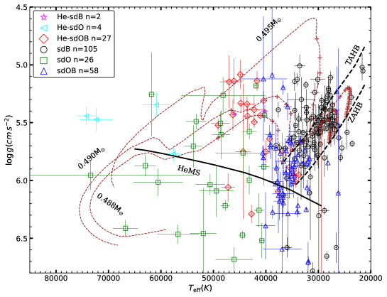
Figure 4: $T_{\rm eff}$-$\log{g}$ diagram for 222 hot subdwarf stars identified in this study. The markers and number counts for different types of hot subdwarfs are shown in the upper-left box. The zero-age horizontal branch (ZAHB) and terminal-age horizontal branch (TAHB) sequences with [Fe/H]= -1.48 from Dorman et al. (1993) are denoted by dashed lines. The He-MS from Paczyński (1971) is marked by black solid line. Three evolution tracks for hot HB stars from Dorman et al. (1993) are presented by brown dotted curves, for which the masses from top to bottom are 0.495, 0.490, and 0.488 $M_{\odot}$, respectively.

Figure 5: $T_{\rm eff}$-$\mathrm{log}(n\mathrm{He}/n\mathrm{H})$ diagram for 222 hot subdwarf identified in this study. The black dotted line and dot-dashed line are the linear regression lines fitted for the two He sequences by Edelmann et al. (2003) and Németh et al. (2012), respectively.

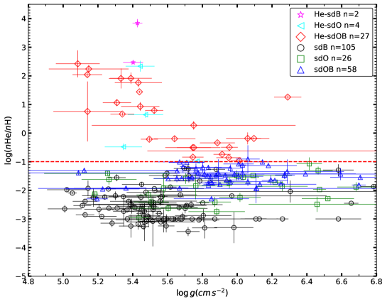
Figure 6: $\log{g}$-$\mathrm{log}(n\mathrm{He}/n\mathrm{H})$ diagram for the 222 hot subdwarfs identified in this study. The red horizontal dashed line denotes the solar value of He abundance (e.g., $\mathrm{log}(n\mathrm{He}/n\mathrm{H})$ = -1).

4.2 Parameter diagrams

The relationships between atmospheric parameters of our 222 samples, e.g., $T_{\mathrm{eff}}$ and $\mathrm{log}\ g$, $T_{\mathrm{eff}}$ and $\mathrm{log}(n\mathrm{He}/n\mathrm{H})$, $\mathrm{log}\ g$ and $\mathrm{log}(n\mathrm{He}/n\mathrm{H})$, are shown in Fig 4 to 6, respectively. Hot subdwarf stars are labeled by different symbols (see legend boxes) in each figure based on their spectral classification. The uncertainties of the parameter values are represented by thin-solid short lines with the same color as symbols.

The relationships between the parameters presented in Fig 4 to 6 are very similar to our previous works (see Lei et al. 2018, 2019b, 2020 for detailed discussion). For example, two He sequences (i.e., a He-rich sequence and a He-poor sequence) are shown very clearly in $T_{\mathrm{eff}}$ - $\mathrm{log}(n\mathrm{He}/n\mathrm{H})$ diagram (see Fig 5), which also have been identified previously by several authors (Edelmann et al., 2003; Németh et al., 2012; Geier et al., 2013; Luo et al., 2016, 2019). Moreover, He-sdOB stars (red open diamonds) are split into two subgroups near at $\mathrm{log}(n\mathrm{He}/n\mathrm{H})$ = 0, which is also presented in our previous work (see Section 5 in Lei et al. 2019b for detailed discussion).

5 discussion and summary

5.1 Two-color diagram

Fig 7 presents the two-color diagram for both composite and single-lined hot subdwarf stars. The u, g and r magnitudes were obtained by crossing-matching our sample with SDSS DR12. The figure clearly shows that composite hot subdwarf stars (red open circles) are well separated from single-lined hot subdwarf stars (blue open squares) in the two-color diagram. These results are consistent with the ones described in Fig 5 of Geier et al. (2017) and Fig 3 of Geier (2020). Note that we selected composite spectra manually based on the presence of obvious Mg I triplet lines at 5170 Å and/or Ca II triplet lines at 8650 Å in the spectra, while Geier (2020) used color criterion in the two-color diagram (e.g., see Table 1 in their study).

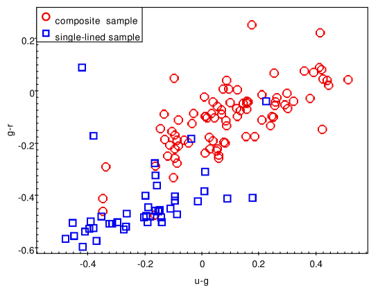
Figure 7: Two-color diagram for hot subdwarfs identified in this study. Only objects having u, g and r photometry from SDSS DR12 are plotted.

Red open circles are hot subdwarf stars identified with composite spectra, while blue open squares are hot subdwarf stars identified with single-lined spectra.

5.2 Two newly discovered wide sdB binaries.

The third data release of the Gaia mission, Gaia DR3, became available to public on 13 June 2022 (Gaia Collaboration et al., 2022). It not only contains astrometric and broad-band photometric information for more than 1.8 billion objects, which have already been published in Gaia EDR3 (Gaia Collaboration et al., 2021), but also presents a large variety of new data products, such as: mean BP, RP and RVS spectra, a much larger radial velocity survey, a large number of variable sources and astrophysical parameters, etc. Especially, Gaia DR3 also contains a non-single star catalog, in which orbital information and trend parameters were solved for more than 800 000 astrometric, spectroscopic, and eclipsing binaries. This catalog provides great convenience to study the binary nature of our composite sample.

We cross-matched our sample of 131 composite spectra with the Gaia DR3 non-single star catalog, and found two common objects (i.e., LAMOST obs_id = 282604062 and 342803178, named as sdB_b1 and sdB_b2 hereafter, respectively). Their information are listed in Table 3. Based on our decomposition results in Table 1, sdB_b1 consists of a sdB primary with $T_{\mathrm{eff}}=27300\pm 430$ K, $\log\mathrm{g}=5.36\pm 0.06$ $\mathrm{cm/s^{-2}}$ and a F2V type cool secondary. While sdB_b2 consists of a sdB primary with $T_{\mathrm{eff}}=27550\pm 90$ K, $\log\mathrm{g}=5.43\pm 0.01$ and a K7V type cool secondary. Based on the data from Gaia DR3, both binary systems have very long orbital periods, i.e., ${\rm P}=884\pm 25$ and ${\rm P}=821\pm 43$ days, respectively (see Table 3). However, the sdB_b1 system has a much higher eccentricity (e.g., ${\rm e}=0.5\pm 0.09$) than sdB_b2 (e.g., ${\rm e}=0.15\pm 0.04$).

Table 3: Two wide sdB binaries identified in this study with solved orbital parameters from Gaia DR3.

Name	RA	DEC	obs_id	source_id	parallax	RUWE	AEN	$G$	Period	Eccentricity
This study	LAMOST	LAMOST	LAMOST	Gaia	Gaia	Gaia	Gaia(mas)	Gaia(mag)	Gaia(days)	Gaia
sdB_b1	4.8358078	46.551897	282604062	392046852459641472	0.4802	1.487	0.21	14.25	884$\pm$25	0.50$\pm$0.09
sdB_b2	261.9515653	16.7492625	342803178	4550114402362108416	1.1289	2.847	0.524	13.48	821$\pm$43	0.15$\pm$0.04

Figure 8: Period-eccentricity plane for wide sdB binaries. Left panel: Known wide sdB binaries are denoted by blue open and black filled circles, while the two newly discovered sdB binaries are shown by red squares. Right panel: same as the left panel, but added prediction area of two physical processes from Vos et al. (2015) and Deca et al. (2018), red for phase-dependent RLOF, while green for CB disk process.

So far, only 23 long-period composite sdB binaries were reported with solved orbital parameters (Vos et al., 2017, 2018, 2019, 2020; Németh et al., 2021; Molina et al., 2022). In Fig 8, we plot known long-orbital period sdB binaries together with the two new discoveries in the period-eccentricity plane. As discussed in other studies (Vos et al., 2017, 2020; Németh et al., 2021), there are two distinct groups among these wide sdB binary systems. This distinction is visible both in the period-eccentricity and the period-mass ratio plane (Vos et al., 2019). The main group (e.g., black filled circles, named Group 1 hereafter) contains most of the binary systems, and all of them present orbital periods longer than 700 days. While the minor group (e.g., blue open circle, named Group 2 hereafter) has only five binary systems, and their orbital periods are shorter than 700 days.

Both two groups show an obvious tendency for higher eccentricities at longer orbital periods, which has not been well explained until now. The left panel of Fig 8 clearly shows, that both of the two new sdB binaries discovered in this study (red filled squares) belong to Group 1 according to their longer orbital periods. However, sdB_b1 presents a very high eccentricity (i.e., e=0.5) that is not only much higher than sdB_b2 (i.e., e=0.15), but also much higher than all other wide sdB binary systems. Therefore, this result places it far away from both Groups 1 and 2. The very high eccentricity demonstrates a different formation or evolution history of this binary, and it needs more detailed and dedicated study in the future. On the other hand, sdB_b2 is consistent with the members of Group 1 in the period-eccentricity plane, which suggests a similar formation history as the main group members.

According to the results from detailed binary population synthesis (Han et al., 2002, 2003; Chen et al., 2013), wide sdB binaries are formed from stable RLOF channel with final orbital periods between 400-1600 days. Nevertheless, these binary systems are predicted with circular orbits before the onset of RLOF, while most of the observed wide sdB binaries present eccentric orbits. There must be some other, yet unclear mechanisms preventing orbital circularization during binary interactions.

Vos et al. (2015) studied the effects of three processes in triggering eccentric orbits during RLOF. They found that phase-dependent mass loss during RLOF and interaction of the binary with a circumbinary (CB) disk could produce eccentric sdB binary systems during RLOF. Deca et al. (2018) extended these models to a wider range of CB-disk properties. In the right panel of Fig 8, the region predicted by phase-dependent RLOF (red area) and CB disk (green area) were added into the period-eccentricity plane. One can see that, most of the binaries from Group 1 (including sdB_b2 discovered in this study) and parts of sdB binaries from Group 2 could be predicted by the models when the two physical processes were considered together. However, there are also several binary systems with shorter orbital periods in Group 2 and higher eccentricities in Group 1 out of the model predictions. Especially, when sdB_b1 is considered, which has the highest eccentricity (i.e., e=0.5) among Groups 1 and 2, the situation becomes even more complicated. Since this binary also presents a much higher eccentricity than the maximum value from the model prediction (e.g., e $\approx$ 0.35 at a period of about 550 days, predicted by the CB disk process). As discussed in Vos et al. (2015) and Németh et al. (2021), sdB binaries present higher eccentricity with longer orbital periods in both two groups, while the two physical processes in Vos et al. (2015) predicted an opposite trend. Furthermore, Oomen et al. (2020) investigated the effect of a CB-disk on the eccentricity of wide post-AGB binaries and found that the Lindbladt resonances between a CB disk and the inner binary are not capable of predicting the observed eccentricities in post-AGB systems.

In the case of the high eccentricity of sdB_b1, it is possible that this system was a triple system where the inner binary merged to produce the current sdB component. The cool companion would then not be involved in the original interaction phase, which could explain the high eccentricity. A detailed study of the abundances of the cool companion as performed by Molina et al. (2022) can provide more insight into this problem. Further observational and theoretical work is needed to uncover the nature of the period-eccentricity distribution for wide sdB binaries.

Figure 9: The period-metallicity plane for wide sdB binaries. Known wide sdB binaries are denoted by blue open circles, while the two newly discovered sdB binaries are shown by red squares. An error of 0.35 in [Fe/H] was assumed for the two new binaries. In green shade, the predicted area of Vos et al. (2020) based on a galactic evolution model coupled with a deterministic binary interaction model.

Vos et al. (2020) investigated the expected wide sdB population using a deterministic binary interaction model including L2 and L3 mass loss coupled with a galactic evolution model. The aim was to explain the period-mass ratio relation found in wide sdB binaries (Vos et al., 2019). This model did not only explain the period-mass ratio relation, but it also predicted a period-metallicity relation originating from the metallicity evolution history in our galaxy. Fig 9 shows the predicted period-metallicity area from the model together with all known observed systems. Both sdB_b1 and sdB_b2 fit well with these predictions, further supporting the validity of the interaction model proposed by Vos et al. (2020). The relevance of this is wider than just sdB binaries, as similar models and approaches are now being used to study the observed populations of other post interaction systems as for example RR Lyr stars (Bobrick et al., 2022) and blue large amplitude pulsators (Xiong et al., 2022).

Figure 10: RUWE-AEN plane for our composite hot subdwarf sample. Objects with AEN $\geq$ 0.4 and RUWE $\geq$ 1.4 are represented by blue open circles, while normal sample are denoted by black pluses. The two nwely discovered sdB binaries are labeled by red filled squares.

5.3 Hints for binarity in composite spectrum hot subdwarf stars.

A high astrometric excess noise (AEN) is a potential signature of physical binary systems. It is defined as the excess uncertainty that must be added in quadrature to obtain a statistically acceptable astrometric solution (Gaia Collaboration et al., 2018a; Lindegren et al., 2012). Higher than expected AEN values might appear in binary systems with unresolved companions. This method was first adopted by Gandhi et al. (2022) to search for X-ray binaries. On the other hand, the Renormalised Unit Weight Error (RUWE) from Gaia data is also considered as a signature for binarity if its value is significantly greater than 1.0 (Lindegren et al., 2018). Uzundag et al. (2022) have combined AEN with RUWE to search for low-mass red giants (RG) binaries, which are also the potential progenitors of sdB stars. They found that more than 90% of the known RG binaries have AEN $\geq$ 0.4, while 93% of known RG binaries have RUWE $\geq$ 1.4. The two values were applied as one of the criteria to search for RG binary candidates in their study.

To provide more hints for the binary nature of our composite hot subdwarf stars, we plotted them in the RUWE-AEN plane. As shown in Fig 10, there are 15 composite sdB stars located in the region with AEN $\geq$ 0.4 and RUWE $\geq$ 1.4, which were labeled as high probability binary candidates (e.g., blue open circles). These systems deserve priority follow-up observations in the future. The two wide sdB binaries identified in this study (e.g., red filled squares) are also presented in the figure. One can see that, sdB_b2 (e.g., AEN=0.524, RUWE=2.847) is well in the high probability binary candidates group. While sdB_b1 is out of this group due to a smaller AEN value of 0.21. But it still presents a large value of RUWE = 1.487, which is also a sign to consider the system as a binary candidate. Based on the results, some hot subdwarf binaries may be hidden in the normal group (e.g., black pluses). In contrast to the RG samples of Uzundag et al. (2022) the RUWE-AEN distribution is less sensitive for binaries in the case of hot subdwarfs as our samples have less luminous stars at larger distances, leading to larger AEN noise and RUWE errors. Yet, according to Fig 10, there are 15 high-probability binary candidates in our sample.

Figure 11: Left panel: $T_{\mathrm{eff}}$-$T_{\mathrm{eff}}$ plane of hot subdwarf primaries vs cool companions for our composite sample. Different labels denote the same groups as in Fig 10. Right panel: Histogram of $T_{\mathrm{eff}}$ distribution for cool companions. Note that both two panels show a distinct gap around at 5500 K among cool companions, see detailed discussions in the context.

Fig 11 presents the relationship of effective temperature ($T_{\mathrm{eff}}$) distribution between hot subdwarf primaries and cool secondaries for our composite sample. The left panel of Fig 11 clearly shows that, both high probability binary candidates (e.g., blue open circles) and normal objects (e.g., black pluses) defined by RUWE-AEN plane in Fig 10 were well separated by a gap among cool secondaries around at 5500 K. To show this feature more clearly, we plotted a histogram of $T_{\mathrm{eff}}$ distribution for all cool secondaries in the right panel. There is indeed a distinct gap around at 5500 K among cool companions. Based on our results of decomposition processes (see Sect 3 and Table 1), most of cool companions in the composite-spectra systems were F, G and K type stars. Therefore, the gap shown in Fig 11 seems to be from the temperatures differences between FG and K type stars.

Interestingly, results from binary population synthesis (BPS) of Han et al. (2003) also predicted a similar gap between the temperature of FG and K type companions for sdB stars produced from the first stable RLOF channel (see panel b and e of Fig 15 in their study). They concluded that the gap was caused by the Hertzsprung gap, since the companions could accrete more masses when the progenitor of sdB stars were in the Hertzsprung gap than the companions with sdB progenitors on the first giant branch (FGB), and tend to be more massive and of earlier spectral type (see detailed discussion in Sect 7.5 of Han et al. 2003). Note that, the hot subdwarf stars with composite spectra presented here were just binary candidates (except for the two newly discovered sdB binary systems). Some of them could be not real binaries, and their companions may be a background or foreground FG or K stars. Hence, we could not obtain a deeper conclusion on this field before the binary nature of the sample are confirmed.

Geier et al. (2022) studied radial velocity (RV) variability for a sample of 646 hot subdwarfs with multi-epoch radial velocities from SDSS and LAMOST. They found that only a small fraction (e.g., $\approx$ 3%, see Section 3 and Fig 2 in their study) of He-rich hot subdwarf stars (i.e., $\mathrm{log}(n\mathrm{He}/n\mathrm{H})\geqslant$ -1) show RV variability, while a much higher fraction of He-poor hot subdwarf stars (i.e., $\mathrm{log}(n\mathrm{He}/n\mathrm{H})<$-1) presents RV variability (e.g., $\approx$ 30%). This striking result led the authors to the conclusion that He-rich and He-poor hot subdwarf stars are evolutionarily not related, and He-rich hot subdwarf stars likely form through the binary merger channel. Considering the results of Pelisoli et al. (2020), single-star evolution has little contribution to the formation of hot subdwarf stars.

Note that, all the stars analyzed by Geier et al. (2022) were single-lined hot subdwarf stars, while composite hot subdwarfs were not included. We cross-matched our 131 composite hot subdwarfs identified with LAMOST DR8 LRS Multiple Epoch Catalog, in which 7,912,959 sources with 2 times or more multiple observations were collected, and found 61 common records. Unfortunately, among these 61 common objects, only two sources have completed RV curves from LAMOST, and the RV variability is low. The lack of RV values for the composite systems prevents us from deriving deeper conclusions in this field. In near future, we plan to use the multi-epoch observed spectra to obtain RV variability of our composite sample, analyze the evolutionary relationships among different hot subdwarf types, and study their binary natures.

5.4 Summary

In this study, we selected 257 composite and 203 single-lined hot subdwarf candidates from LAMOST DR8 dataset with the help of Gaia EDR3 H-R diagram and the catalog of Geier et al. (2019). 222 stars were confirmed as hot subdwarfs, among which 131 objects were identified with composite spectra, and 91 objects with single-lined spectra. We cross-matched our sample with the hot subdwarf star catalog of Geier (2020), and confirmed that 74 hot subdwarf stars in our sample are new discoveries. Though 148 stars have been recorded before, 109 of them were reported without atmospheric parameters. We obtained their atmospheric parameters by fitting the H and He line profiles with synthetic spectra. Composite hot subdwarfs are well separated from single-lined hot subdwarfs in the two-color diagram. Two wide sdB binaries with composite spectra were discovered, sdB_b1 and sdB_b2. Their long orbital periods (i.e., $884\pm 25$ and $821\pm 43$ days, respectively) make them belong to the main group of known wide sdB binaries. However, sdB_b1 shows the highest eccentricity among these binaries, which is far beyond model predictions. Further study is expected before the nature of period-eccentricity for wide sdB binaries is clearly understood. Our sample reported here are valuable resources to carry out spectroscopic follow-up observations, especially for the 15 composite sdB stars falling in the highly reliable binary region of RUWE-AEN plane. A distinct gap is clearly presented among temperatures of cool companions for the composite sample, but it is a little early to come into the conclusion that this feature is related to the formation history of hot subdwarf stars before their binary natures are confirmed.

References

- Abolfathi et al. (2018) Abolfathi, B., Aguado, D. S., Aguilar, G., et al. 2018, ApJS, 235, 42, doi: 10.3847/1538-4365/aa9e8a
- Astropy Collaboration et al. (2013) Astropy Collaboration, Robitaille, T. P., Tollerud, E. J., et al. 2013, A&A, 558, A33, doi: 10.1051/0004-6361/201322068
- Astropy Collaboration et al. (2018) Astropy Collaboration, Price-Whelan, A. M., Sipőcz, B. M., et al. 2018, AJ, 156, 123, doi: 10.3847/1538-3881/aabc4f
- Bobrick et al. (2022) Bobrick, A., Iorio, G., Belokurov, V., et al. 2022, arXiv e-prints, arXiv:2208.04332. https://arxiv.org/abs/2208.04332
- Bohlin et al. (2017) Bohlin, R. C., Mészáros, S., Fleming, S. W., et al. 2017, AJ, 153, 234, doi: 10.3847/1538-3881/aa6ba9
- Bu et al. (2017) Bu, Y., Lei, Z., Zhao, G., Bu, J., & Pan, J. 2017, ApJS, 233, 2, doi: 10.3847/1538-4365/aa91cd
- Bu et al. (2019) Bu, Y., Zeng, J., Lei, Z., & Yi, Z. 2019, ApJ, 886, 128, doi: 10.3847/1538-4357/ab4c47
- Chen et al. (2013) Chen, X., Han, Z., Deca, J., & Podsiadlowski, P. 2013, MNRAS, 434, 186, doi: 10.1093/mnras/stt992
- Clausen & Wade (2011) Clausen, D., & Wade, R. A. 2011, ApJ, 733, L42, doi: 10.1088/2041-8205/733/2/L42
- Cui et al. (2012) Cui, X.-Q., Zhao, Y.-H., Chu, Y.-Q., et al. 2012, Research in Astronomy and Astrophysics, 12, 1197, doi: 10.1088/1674-4527/12/9/003
- Culpan et al. (2022) Culpan, R., Geier, S., Reindl, N., et al. 2022, A&A, 662, A40, doi: 10.1051/0004-6361/202243337
- Deca et al. (2018) Deca, J., Vos, J., Németh, P., et al. 2018, MNRAS, 474, 433, doi: 10.1093/mnras/stx2755
- Deca et al. (2012) Deca, J., Marsh, T. R., Østensen, R. H., et al. 2012, MNRAS, 421, 2798, doi: 10.1111/j.1365-2966.2012.20483.x
- Dorman et al. (1993) Dorman, B., Rood, R. T., & O’Connell, R. W. 1993, ApJ, 419, 596, doi: 10.1086/173511
- Dorsch et al. (2021) Dorsch, M., Jeffery, C. S., Irrgang, A., Woolf, V., & Heber, U. 2021, A&A, 653, A120, doi: 10.1051/0004-6361/202141381
- Edelmann et al. (2003) Edelmann, H., Heber, U., Hagen, H. J., et al. 2003, A&A, 400, 939, doi: 10.1051/0004-6361:20030135
- Gaia Collaboration et al. (2016) Gaia Collaboration, Prusti, T., de Bruijne, J. H. J., et al. 2016, A&A, 595, A1, doi: 10.1051/0004-6361/201629272
- Gaia Collaboration et al. (2018a) Gaia Collaboration, Brown, A. G. A., Vallenari, A., et al. 2018a, A&A, 616, A1, doi: 10.1051/0004-6361/201833051
- Gaia Collaboration et al. (2018b) Gaia Collaboration, Babusiaux, C., van Leeuwen, F., et al. 2018b, A&A, 616, A10, doi: 10.1051/0004-6361/201832843
- Gaia Collaboration et al. (2021) Gaia Collaboration, Brown, A. G. A., Vallenari, A., et al. 2021, A&A, 649, A1, doi: 10.1051/0004-6361/202039657
- Gaia Collaboration et al. (2022) Gaia Collaboration, Vallenari, A., Brown, A. G. A., et al. 2022, arXiv e-prints, arXiv:2208.00211. https://arxiv.org/abs/2208.00211
- Gandhi et al. (2022) Gandhi, P., Buckley, D. A. H., Charles, P. A., et al. 2022, MNRAS, 510, 3885, doi: 10.1093/mnras/stab3771
- Geier (2020) Geier, S. 2020, A&A, 635, A193, doi: 10.1051/0004-6361/202037526
- Geier et al. (2022) Geier, S., Dorsch, M., Pelisoli, I., et al. 2022, arXiv e-prints, arXiv:2202.09608. https://arxiv.org/abs/2202.09608
- Geier et al. (2013) Geier, S., Heber, U., Edelmann, H., et al. 2013, A&A, 557, A122, doi: 10.1051/0004-6361/201322057
- Geier et al. (2017) Geier, S., Østensen, R. H., Nemeth, P., et al. 2017, A&A, 600, A50, doi: 10.1051/0004-6361/201630135
- Geier et al. (2019) Geier, S., Raddi, R., Gentile Fusillo, N. P., & Marsh, T. R. 2019, A&A, 621, A38, doi: 10.1051/0004-6361/201834236
- Green et al. (2001) Green, E. M., Liebert, J., & Saffer, R. A. 2001, in Astronomical Society of the Pacific Conference Series, Vol. 226, 12th European Workshop on White Dwarfs, ed. J. L. Provencal, H. L. Shipman, J. MacDonald, & S. Goodchild, 192. https://arxiv.org/abs/astro-ph/0012246
- Han et al. (2003) Han, Z., Podsiadlowski, P., Maxted, P. F. L., & Marsh, T. R. 2003, MNRAS, 341, 669, doi: 10.1046/j.1365-8711.2003.06451.x
- Han et al. (2002) Han, Z., Podsiadlowski, P., Maxted, P. F. L., Marsh, T. R., & Ivanova, N. 2002, MNRAS, 336, 449, doi: 10.1046/j.1365-8711.2002.05752.x
- Heber (1986) Heber, U. 1986, A&A, 155, 33
- Heber (2009) —. 2009, ARA&A, 47, 211, doi: 10.1146/annurev-astro-082708-101836
- Heber (2016) —. 2016, PASP, 128, 082001, doi: 10.1088/1538-3873/128/966/082001
- Hubeny & Lanz (2017) Hubeny, I., & Lanz, T. 2017, arXiv e-prints, arXiv:1706.01859. https://arxiv.org/abs/1706.01859
- Kepler et al. (2019) Kepler, S. O., Pelisoli, I., Koester, D., et al. 2019, MNRAS, 486, 2169, doi: 10.1093/mnras/stz960
- Lanz & Hubeny (2007) Lanz, T., & Hubeny, I. 2007, ApJS, 169, 83, doi: 10.1086/511270
- Lei et al. (2019a) Lei, Z., Bu, Y., Zhao, J., Németh, P., & Zhao, G. 2019a, PASJ, 71, 41, doi: 10.1093/pasj/psz006
- Lei et al. (2015) Lei, Z., Chen, X., Zhang, F., & Han, Z. 2015, MNRAS, 449, 2741, doi: 10.1093/mnras/stv544
- Lei et al. (2016) Lei, Z., Zhao, G., Zeng, A., et al. 2016, MNRAS, 463, 3449, doi: 10.1093/mnras/stw2242
- Lei et al. (2018) Lei, Z., Zhao, J., Németh, P., & Zhao, G. 2018, ApJ, 868, 70, doi: 10.3847/1538-4357/aae82b
- Lei et al. (2019b) —. 2019b, ApJ, 881, 135, doi: 10.3847/1538-4357/ab2edc
- Lei et al. (2020) —. 2020, ApJ, 889, 117, doi: 10.3847/1538-4357/ab660a
- Lindegren et al. (2012) Lindegren, L., Lammers, U., Hobbs, D., et al. 2012, A&A, 538, A78, doi: 10.1051/0004-6361/201117905
- Lindegren et al. (2018) Lindegren, L., Hernández, J., Bombrun, A., et al. 2018, A&A, 616, A2, doi: 10.1051/0004-6361/201832727
- Luo et al. (2019) Luo, Y., Németh, P., Deng, L., & Han, Z. 2019, ApJ, 881, 7, doi: 10.3847/1538-4357/ab298d
- Luo et al. (2021) Luo, Y., Németh, P., Wang, K., Wang, X., & Han, Z. 2021, ApJS, 256, 28, doi: 10.3847/1538-4365/ac11f6
- Luo et al. (2016) Luo, Y.-P., Németh, P., Liu, C., Deng, L.-C., & Han, Z.-W. 2016, ApJ, 818, 202, doi: 10.3847/0004-637X/818/2/202
- Mészáros et al. (2012) Mészáros, S., Allende Prieto, C., Edvardsson, B., et al. 2012, AJ, 144, 120, doi: 10.1088/0004-6256/144/4/120
- Moehler et al. (1990) Moehler, S., Richtler, T., de Boer, K. S., Dettmar, R. J., & Heber, U. 1990, A&AS, 86, 53
- Molina et al. (2022) Molina, F., Vos, J., Németh, P., et al. 2022, A&A, 658, A122, doi: 10.1051/0004-6361/202141220
- Németh et al. (2012) Németh, P., Kawka, A., & Vennes, S. 2012, MNRAS, 427, 2180, doi: 10.1111/j.1365-2966.2012.22009.x
- Nemeth et al. (2014) Nemeth, P., Östensen, R., Tremblay, P., & Hubeny, I. 2014, in Astronomical Society of the Pacific Conference Series, Vol. 481, 6th Meeting on Hot Subdwarf Stars and Related Objects, ed. V. van Grootel, E. Green, G. Fontaine, & S. Charpinet, 95. https://arxiv.org/abs/1308.0252
- Németh et al. (2021) Németh, P., Vos, J., Molina, F., & Bastian, A. 2021, A&A, 653, A3, doi: 10.1051/0004-6361/202141442
- Oomen et al. (2020) Oomen, G.-M., Pols, O., Van Winckel, H., & Nelemans, G. 2020, A&A, 642, A234, doi: 10.1051/0004-6361/202038341
- Østensen & Van Winckel (2012) Østensen, R. H., & Van Winckel, H. 2012, in Astronomical Society of the Pacific Conference Series, Vol. 452, Fifth Meeting on Hot Subdwarf Stars and Related Objects, ed. D. Kilkenny, C. S. Jeffery, & C. Koen, 163. https://arxiv.org/abs/1112.0977
- Paczyński (1971) Paczyński, B. 1971, Acta Astron., 21, 1
- Pelisoli et al. (2020) Pelisoli, I., Vos, J., Geier, S., Schaffenroth, V., & Baran, A. S. 2020, A&A, 642, A180, doi: 10.1051/0004-6361/202038473
- Tan et al. (2022) Tan, L., Mei, Y., Liu, Z., et al. 2022, ApJS, 259, 5, doi: 10.3847/1538-4365/ac4de8
- Taylor (2005) Taylor, M. B. 2005, in Astronomical Society of the Pacific Conference Series, Vol. 347, Astronomical Data Analysis Software and Systems XIV, ed. P. Shopbell, M. Britton, & R. Ebert, 29
- Uzundag et al. (2022) Uzundag, M., Jones, M. I., Vučković, M., et al. 2022, arXiv e-prints, arXiv:2209.08971. https://arxiv.org/abs/2209.08971
- Vos et al. (2020) Vos, J., Bobrick, A., & Vučković, M. 2020, A&A, 641, A163, doi: 10.1051/0004-6361/201937195
- Vos et al. (2018) Vos, J., Németh, P., Vučković, M., Østensen, R., & Parsons, S. 2018, MNRAS, 473, 693, doi: 10.1093/mnras/stx2198
- Vos et al. (2015) Vos, J., Østensen, R. H., Marchant, P., & Van Winckel, H. 2015, A&A, 579, A49, doi: 10.1051/0004-6361/201526019
- Vos et al. (2017) Vos, J., Østensen, R. H., Vučković, M., & Van Winckel, H. 2017, A&A, 605, A109, doi: 10.1051/0004-6361/201730958
- Vos et al. (2019) Vos, J., Vučković, M., Chen, X., et al. 2019, MNRAS, 482, 4592, doi: 10.1093/mnras/sty3017
- Vos et al. (2012) Vos, J., Østensen, R. H., Degroote, P., et al. 2012, A&A, 548, A6, doi: 10.1051/0004-6361/201219723
- Xiong et al. (2022) Xiong, H., Casagrande, L., Chen, X., et al. 2022, A&A, forthcoming, doi: 10.1051/0004-6361/202244571
- Zhang et al. (2017) Zhang, X., Hall, P. D., Jeffery, C. S., & Bi, S. 2017, ApJ, 835, 242, doi: 10.3847/1538-4357/835/2/242
- Zhang & Jeffery (2012) Zhang, X., & Jeffery, C. S. 2012, MNRAS, 419, 452, doi: 10.1111/j.1365-2966.2011.19711.x
- Zhao et al. (2006) Zhao, G., Chen, Y.-Q., Shi, J.-R., et al. 2006, Chinese J. Astron. Astrophys., 6, 265, doi: 10.1088/1009-9271/6/3/01
- Zhao et al. (2012) Zhao, G., Zhao, Y.-H., Chu, Y.-Q., Jing, Y.-P., & Deng, L.-C. 2012, Research in Astronomy and Astrophysics, 12, 723, doi: 10.1088/1674-4527/12/7/002