Randomized sketching of nonlinear eigenvalue problems

Abstract

Rational approximation is a powerful tool to obtain accurate surrogates for nonlinear functions that are easy to evaluate and linearize. The interpolatory adaptive Antoulas–Anderson (AAA) method is one approach to construct such approximants numerically. For large-scale vector- and matrix-valued functions, however, the direct application of the set-valued variant of AAA becomes inefficient. We propose and analyze a new sketching approach for such functions called sketchAAA that, with high probability, leads to much better approximants than previously suggested approaches while retaining efficiency. The sketching approach works in a black-box fashion where only evaluations of the nonlinear function at sampling points are needed. Numerical tests with nonlinear eigenvalue problems illustrate the efficacy of our approach, with speedups above 200 for sampling large-scale black-box functions without sacrificing on accuracy.

1 Introduction

This work is concerned with approximating vector-valued and matrix-valued functions, with a particular focus on functions $F\colon\Sigma\to\mathbb{C}^{n\times n}$ that arise in the context of nonlinear eigenvalue problems (NLEVP)

$$F(z)\mathbf{v}=0,\quad\mathbf{v}\not=0.$$ (1)

Recent algorithmic advances have made it possible to efficiently compute an accurate rational approximant of a scalar function $f\colon\Sigma\to{\mathbb{C}}$ on a compact (and usually discrete) target set $\Sigma$ in the complex plane ${\mathbb{C}}$. Some of the available methods are the adaptive Antoulas–Anderson (AAA) algorithm [17], the rational Krylov fitting (RKFIT) algorithm [1], vector fitting [9], minimal rational interpolation [19], and methods based on Löwner matrices [15]. All of these methods can be used or adapted to approximate multiple scalar functions $f_{1},\ldots,f_{s}$ on the target set $\Sigma$ simultaneously. In particular, there are several variants of AAA that approximate multiple functions by a family of rational interpolants sharing the same denominator, including the set-valued AAA algorithm [14], fastAAA [13], and weighted AAA [18]. See also [6] for a discussion and comparison of some of these methods.

AAA-type algorithms can be used with very little user input and have enabled an almost black-box approximation of NLEVPs or transfer functions in model order reduction. However, the computation of $s$ degree-$d$ rational interpolants via the set-valued AAA algorithm involves the solution of $d$ least squares problems with dense matrices of sizes $s(|\Sigma|-k-1)\times(k+1)$ for varying $k=1,2,\ldots,d$, adding up to $O(s|\Sigma|d^{3})$ complexity. The greedy search of interpolation nodes in AAA also requires the repeated evaluation of the $s$ rational interpolants at all sampling points in $\Sigma$ and the storage of the corresponding function values. As a consequence, the main use case for the multiple-function AAA variants to date have been problems that can be written in the split form

$$F(z)=\sum_{i=1}^{s}f_{i}(z)A_{i},$$ (2)

where $s$ is small (say, in the order of $s\approx 10$), $f_{i}$ are known scalar functions, and $A_{i}\in\mathbb{C}^{m\times n}$ are fixed coefficient matrices. While, in principle, it is always possible to write an arbitrary $m\times n$ matrix-valued function $F$ in split form using $s=mn$ terms, it would be prohibitive to apply the set-valued AAA approach to large-scale problems in such a naive way.

The work [5] suggested an alternative approach where the original (scalar-valued) AAA algorithm is applied to a scalar surrogate $f(z)=\mathbf{u}^{T}F(z)\mathbf{v}$ with random probing vectors $\mathbf{u}$ and $\mathbf{v}$, resulting in a rational interpolant in barycentric form

$$r^{(d)}(z)=\sum_{i=0}^{d}\frac{w_{i}\,f(z_{i})}{z-z_{i}}\bigg{/}\sum_{i=0}^{d}\frac{w_{i}}{z-z_{i}}$$ (3)

with support points $z_{i}\in{\mathbb{C}}$ (the interpolation nodes) and weights $w_{i}\in{\mathbb{C}}$. Using this representation, a rational interpolant $R^{(d)}$ of the original function $F$ is then obtained by replacing in (3) every occurrence of $f(z_{i})$ by the evaluation $F(z_{i})$:

$$R^{(d)}(z)=\sum_{i=0}^{d}\frac{w_{i}\,F(z_{i})}{z-z_{i}}\bigg{/}\sum_{i=0}^{d}\frac{w_{i}}{z-z_{i}}.$$ (4)

The intuition is that both $F$ and $f$ will almost surely have the same region of analyticity, hence interpolating $F$ using the same interpolation nodes and poles as for $f$ should result in a good approximant. This surrogate approach indeed alleviates the complexity and memory issues even when $F$ has a large number of terms $s$ in its split form (2), and it can also be applied if $F$ is only available as a black-box function returning evaluations $z\mapsto F(z)$. However, a comprehensive numerical comparison in [18] in the context of solving NLEVPs (1) has revealed that this surrogate approach is not always reliable and may lead to poor accuracy. Indeed, the $\Sigma$-uniform error for the original problem

$$\|F-R^{(d)}\|_{\Sigma}:=\max_{z\in\Sigma}\|F(z)-R^{(d)}(z)\|_{F}$$ (5)

can be significantly larger than the error for the scalar surrogate problem $\|f-r^{(d)}\|_{\Sigma}$. In order to mitigate this issue for black-box functions $F(z)$—i.e., those not available in split form (2)—a two-phase surrogate AAA algorithm with cyclic Leja–Bagby refinement has been developed in [18]. While this algorithm is indeed robust in the sense that it returns a rational approximant with user-specified accuracy, it is computationally more expensive than the set-valued AAA algorithm and sometimes returns approximants of unnecessarily high degree; see, e.g., [18, Table 5.2].

In this work, we propose and analyze a new sketching approach for matrix-valued functions called sketchAAA that, with high probability, leads to much better approximants than the scalar surrogate AAA approach. At the same time, it remains equally efficient. While we demonstrate the benefits of the sketching approach in combination with the set-valued AAA algorithm and mainly test it on functions from the updated NLEVP benchmark collection [2, 12], the same technique can be combined with other linear interpolation techniques (including polynomial interpolation at adaptively chosen nodes). Our sketching approach is not limited to nonlinear eigenvalue problems either and can be used for the approximation of any vector-valued function. The key idea is to sketch $\mathbf{f}(z)={\mathrm{vec}}(F(z))$ using a thin (structured or unstructured) random probing matrix $V\in{\mathbb{C}}^{N\times\ell}$, i.e., computing samples of the form $V^{T}\mathbf{f}(z_{i})$, and then to apply the set-valued AAA algorithm to the $\ell$ components of the samples. We provide a probabilistic assessment of the approximation quality of the resulting samples by building on the improved small-sample bounds of the matrix Frobenius norm in [7].

The remainder of this work is organized as follows. In section 2 we briefly review the AAA algorithm [17] and the surrogate approach from [5], and then introduce our new probing forms using either tensorized or non-tensorized probing vectors. We also provide a pseudocode of the resulting sketchAAA algorithm. Section 3 is devoted to the analysis of the approximants produced by sketchAAA ​​. Our main result for the case of non-tensorized probing, Theorem 3.2, provides an exponentially converging (in the number of samples $\ell$) probabilistic upper bound on the approximation error of the sketched problem compared to the approximation of the full problem. We also provide a weaker result for tensorized probing in the case of $\ell=1$, covering the original surrogate approach in [5]. Several numerical tests in section 4 on small to large-scale problems show that our new sketching approach is reliable and efficient. For some of the large-scale black-box problems we report speedup factors above 200 compared to the set-valued AAA algorithm while retaining comparable accuracy.

2 Surrogate functions and the AAA algorithm

The AAA algorithm [17] is a relatively simple but usually very effective method for obtaining a good rational approximant $r^{(d)}(z)\approx f(z)$ of the form (3) for a given function $f\colon{\mathbb{C}}\supset\Omega\to{\mathbb{C}}$. The approximation is sought on a finite discretization $\Sigma\subset\Omega$ and discretization sizes of $|\Sigma|\approx 10^{3}$–$10^{4}$ are not uncommon. The method iteratively selects support points (interpolation nodes) by adding to a previously computed set $\{z_{0},z_{1},\ldots,z_{d-1}\}$ of $d$ support points a new point $z_{d}\in\Sigma$ at which $\max_{z\in\Sigma}|r^{(d-1)}(z)-f(z)|$ is attained. After that, the rational approximant $r^{(d)}$ is calculated by computing $d+1$ weights $w_{i}\in{\mathbb{C}}$ as the minimizer of the linearized approximation error

$$\min_{\mathbf{w}\in\mathbb{C}^{d+1}}\|L\mathbf{w}\|_{2}\quad\text{such that}\quad\|\mathbf{w}\|_{2}=1.$$ (6)

Here, $L$ is a Löwner matrix of size $(|\Sigma|-d-1)\times(d+1)$ defined as

$$L_{ij}=\frac{f(\hat{z}_{i})-f(z_{j})}{\hat{z}_{i}-z_{j}}$$ (7)

where $\{\hat{z}_{1},\hat{z}_{2},\ldots\}=\Sigma\setminus\{z_{0},\ldots,z_{d}\}$. The minimization problem (6) can be solved exactly by SVD at a cost of $O(|\Sigma|d^{2})$ flops. Since the matrix $L$ is only altered in one row and column after each iteration, updating strategies can be used to lower the computational cost of its SVD; see, e.g., [13, 14]. However, the numerical stability of such updating strategies is not guaranteed.

It is not difficult to extend AAA for the approximation of a vector-valued function $\mathbf{f}\colon\Omega\to{\mathbb{C}}^{N}$. Firstly, the vector-valued version $\mathbf{r}^{(d)}$ of (3) will map into ${\mathbb{C}}^{N}$ since the $\mathbf{f}(z_{i})$ are vector-valued. However, the support points $z_{i}$ and weights $w_{i}$ remain scalars. The selection of the support points can still be done greedily by, at iteration $d$, choosing a support point $z_{d}\in\Sigma$ that maximizes $\|\mathbf{r}^{(d-1)}(z)-\mathbf{f}(z)\|$ on $\Sigma$ for some norm $\|\cdot\|$. In practice, the infinity or Euclidean norm usually work well but more care is sometimes needed when $\mathbf{f}$ maps to different scales; see [14, 18]. Likewise, the weights are computed from a block-Löwner matrix $L$ where each $L_{ij}$ in (7) is now a column vector of length $N$ composed with $\mathbf{f}(\hat{z}_{i}),\mathbf{f}(z_{j})\in{\mathbb{C}}^{N}$. The matrix $L$ is now of size $N(|\Sigma|-d-1)\times(d+1)$, increasing the cost of its SVD to $O(N|\Sigma|d^{2})$ flops. When computing these SVDs for degrees $1,2,\ldots,d$ as is required by AAA, the cumulative cost is $(N|\Sigma|d^{3})$. For large $N$, this becomes prohibitive.

As explained in the introduction, a way to lower the computational cost for s vector-valued function $\mathbf{f}$ is to work with a scalar surrogate function $g\colon\Omega\to{\mathbb{C}}$ that hopefully shares the same region of analyticity as $\mathbf{f}$. In [5] this function was chosen with a tensorized probing vector:

$$g_{\text{tens}}(z)=(\mathbf{v}\otimes\mathbf{u})^{T}\mathbf{f}(z)\quad\text{with fixed random vectors $\mathbf{u},\mathbf{v}\in{\mathbb{C}}^{n}$}.$$ (8)

The reason for this construction with a tensor product is that [5] focused on nonlinear eigenvalue problems where $\mathbf{f}(z)={\mathrm{vec}}(F(z))$ with $F(z)\in{\mathbb{C}}^{n\times n}$. This allows for an efficient evaluation $g_{\text{tens}}(z)=\mathbf{u}^{T}F(z)\mathbf{v}$, which becomes particularly advantageous when fast matrix-vector products with $F(z)$ are available. In the case that $F$ is in the split form (2), only a matrix-vector product with each $A_{i}$ is needed. A similar surrogate can be obtained for general $\mathbf{f}\colon\Omega\to{\mathbb{C}}^{N}$ by using a full (non-tensorized) probing vector:

$$g_{\text{full}}(z)=\mathbf{v}^{T}\mathbf{f}(z)\quad\text{with a fixed random vector $\mathbf{v}\in\mathbb{C}^{N}$.}$$ (9)

For both surrogate constructions, we apply AAA to $g_{\text{tens}}$ or $g_{\text{full}}$ and use the computed support points $z_{i}$ and weights $w_{i}$ to define $\mathbf{r}^{(d)}$ as in (3), replacing the scalar function values by the vectors $\mathbf{f}(z_{i})$. Since the surrogate functions $g_{\text{tens}}$ are $g_{\text{full}}$ are scalar-valued, the computational burden is clearly much lower than applying the set-valued AAA method to the vector-valued function $\mathbf{f}$.

While computationally very attractive, the approach of building a scalar surrogate does unfortunately not always result in very accurate approximants. To illustrate, we consider the matrix-valued function $F$ of the buckling_plate example from [12]. In Figure 1 the errors for both surrogates (8) and (9) are shown in blue. While AAA fully resolves each surrogate to an absolute accuracy well below $10^{-10}$, the absolute errors of the corresponding matrix-valued approximants to $F$ stagnate around $10^{-5}$.

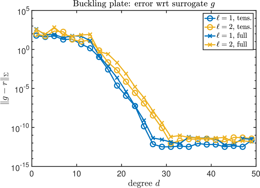
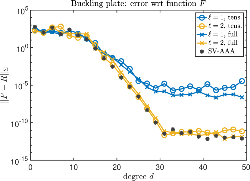
Figure 1: Approximation errors of the rational interpolant for the buckling_plate example as functions of the degree $d$. The error of the surrogate functions ($\ell=1$ or $\ell=2$ probing vectors, tensorized or not) is shown in the left panel, and on the right the error of the full interpolants is shown. While the errors of the surrogates all converge to machine precision (left), the error of the full interpolants stagnates when scalar surrogates ($\ell=1$) are used (right). With $\ell=2$ probing vectors the surrogate and full approximants converge similarly. On the right, the error of the set-valued AAA approximant applied the nine components of the original function $F$ is indicated with dark grey dots.

An important observation put forward in this paper is that by taking multiple random probing vectors (and thereby a vector-valued surrogate function $\mathbf{g}$), the approximation error obtained with the set-valued AAA method can be improved, sometimes dramatically. In particular, we consider

$$\mathbf{g}_{\ell,\text{full}}(z)=V^{T}\mathbf{f}(z)\quad\text{with a random matrix $V\in{\mathbb{C}}^{N\times\ell}$}$$ (10)

and the tensorized version

$$\mathbf{g}_{\ell,\text{tens}}(z)=[\mathbf{v}_{1}\otimes\mathbf{u}_{1},\ldots,\mathbf{v}_{\ell}\otimes\mathbf{u}_{\ell}]^{T}\mathbf{f}(z)\quad\text{with random vectors $\mathbf{u}_{i},\mathbf{v}_{i}\in{\mathbb{C}}^{n}$}.$$ (11)

Both probing variants can be sped up if $F(z)$ (and hence $\mathbf{f}(z)$) is available in the split form (2) by precomputing the products of the random vectors with the matrices $A_{1},\ldots,A_{s}$. The tensorized variant is computationally attractive when matrix vector products with $F(z)$ can be computed efficiently since $(\mathbf{v}_{i}\otimes\mathbf{u}_{i})^{T}\mathbf{f}(z)$ is the vectorization of $\mathbf{u}_{i}^{T}F(z)\mathbf{v}_{i}$. In both cases we obtain a vector-valued function with $\ell\ll N$ components to which the set-valued AAA method can readily be applied. The resulting algorithm sketchAAA is summarized in Algorithm 1.

Algorithm 1 AAA with random sketching (sketchAAA)

Nonlinear function $\mathbf{f}\colon\mathbb{C}\supset\Sigma\to\mathbb{C}^{N}$. Number of probing vectors $\ell$. Degree of approximation $d$.

1. Draw a random probing matrix $V\in{\mathbb{C}}^{N\times\ell}$.

2. Define (and possibly precompute on $\Sigma$) the surrogate $\mathbf{g}_{\ell}(z)=V^{T}\mathbf{f}(z)$.

3. Approximate $\mathbf{g}_{\ell}$ on $\Sigma$ using the set-valued AAA method, resulting in a rational function in barycentric form with weights $\{w_{i}\}_{i=0}^{d}$ and support points $\{z_{i}\}_{i=0}^{d}$.

4. Return the rational approximant of $\mathbf{f}$ in the form

$$\mathbf{r}^{(d)}(z)=\sum_{i=0}^{d}\frac{w_{i}\,\mathbf{f}(z_{i})}{z-z_{i}}\bigg{/}\sum_{i=0}^{d}\frac{w_{i}}{z-z_{i}}.$$

Sometimes using as little as $\ell=2$ probing vectors leads to very satisfactory results. This is indeed the case for our example in Figure 1 where the approximation errors of both surrogates (10) and (11) are shown in orange. Both approximants converge rapidly to an absolute error below $10^{-10}$. Remarkably, the approximation error of the surrogates is essentially identical to the error of set-valued AAA approximant applied to the original function $F$, which maps to ${\mathbb{C}}^{3\times 3}$; see Figure 1 (right).

Since the surrogates are random, the resulting rational approximants are also random. Fortunately, their approximation errors concentrate quickly. This is clearly visible in Figure 2 for the bucking_plate and nep2 examples from the NLEVP collection, showing the the 50-percentiles which are less than $10^{-1}$ wide. As a result, the random construction of the surrogates yields rational approximants that, with high probability, all have very similar approximation errors. Figure 2 also demonstrates that two probing vectors do not always suffice. For the nep2 problem, $\ell=4$ probing vectors are required for a relative approximation error close to machine precision.

Many more such examples are discussed in section 4 and in almost all cases a relatively small number $\ell$ of probing vectors suffices to obtain accurate approximations. The next section provides some theoretical insights into this.

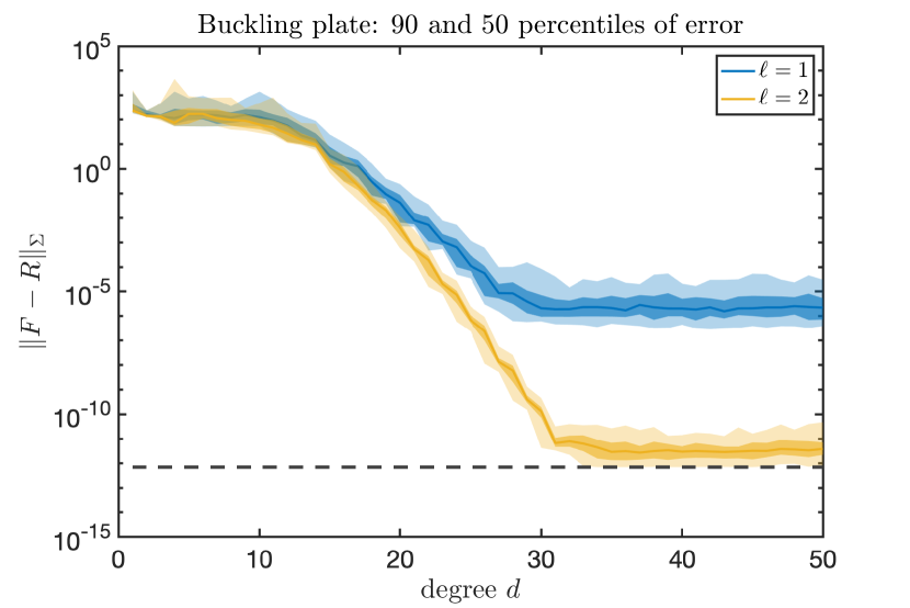
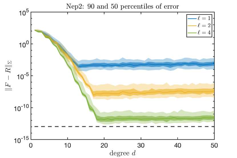
Figure 2: Bands for the 90 and 50 percentiles of 100 random initializations of the surrogates (non-tensorized) for the buckling_plate and nep2 examples. The dashed line is the minimal error achieved by the set-valued AAA method applied to the original function $F$.

3 Analysis of random sketching for function approximation

In this section we analyze the effect of random sketching on the approximation error. More precisely, we show that for a given fixed approximation of $\mathbf{f}$ the corresponding approximation of the sketch $V^{T}\mathbf{f}$ enjoys, with high probability, similar accuracy. Let us emphasize that this setting does not fully capture Algorithm 1 because the approximation constructed by the algorithm depends on the random matrix $V$ in a highly nontrivial way. Nevertheless, we feel that the analysis explains the behavior of the algorithm for increasing $\ell$ and, more concretely, it allows us to cheaply and safely estimate the full error a posteriori via a surrogate (with an independent sketch).

3.1 Preliminaries

Let us consider a vector-valued function $\mathbf{h}\colon\Omega\to\mathbb{K}^{N}$ on some domain $\Omega\subseteq\mathbb{C}$ and with $\mathbb{K}\in\{\mathbb{R},\mathbb{C}\}$. Assuming $\mathbf{h}\in L^{2}(\Omega,{\mathbb{K}}^{N})$ we can equivalently view $\mathbf{h}$ as an element of the tensor product space ${\mathbb{K}}^{N}\otimes L^{2}(\Omega,\mathbb{K})$ that induces the linear operator $\mathcal{L}_{h}\colon L^{2}(\Omega,\mathbb{K})\to{\mathbb{K}}^{N}$, $\mathcal{L}_{h}\colon v\mapsto\int_{\Omega}h(z)v(z)\,\mathrm{d}z$. Note that $\mathcal{L}_{h}$ is a Hilbert–Schmidt operator of rank at most $N$. Applying the Schmidt decomposition [11, Theorem 4.137] implies the following result.

Theorem 3.1.

Let $\mathbf{h}\in L^{2}(\Omega,{\mathbb{K}}^{N})$. There exist orthonormal vectors $\mathbf{u}_{1},\ldots,\mathbf{u}_{N}\in{\mathbb{K}}^{N}$, orthonormal functions $v_{1},\ldots,v_{N}\in L^{2}(\Omega,\mathbb{K})$, and scalars $\sigma_{1}\geq\sigma_{2}\geq\cdots\geq\sigma_{N}\geq 0$ such that

$$\mathbf{h}(z)=\sum_{j=1}^{N}\sigma_{j}\mathbf{u}_{j}v_{j}(z).$$

We note that the singular values $\sigma_{1},\ldots,\sigma_{N}$ are uniquely defined by $\mathbf{h}$. By Theorem 3.1, the norm of $\mathbf{h}$ on $L^{2}(\Omega,{\mathbb{K}}^{N})$ satisfies

$$\|\mathbf{h}\|^{2}:=\int_{\Omega}\|\mathbf{h}(z)\|_{2}^{2}\,\mathrm{d}z=\sigma_{1}^{2}+\cdots+\sigma_{N}^{2},$$

where $\|\cdot\|_{2}$ denotes the Euclidean norm of a vector. Extending the corresponding notion for matrices, the stable rank of $\mathbf{h}$ is defined as $\rho:=\|\mathbf{h}\|^{2}/\sigma_{1}^{2}$ and satisfies $1\leq\rho\leq N$.

Our analysis applies to an abstract approximation operator $\mathcal{A}:\mathcal{W}\to L^{2}(\Omega,{\mathbb{K}}^{N})$ defined on some subspace $\mathcal{W}\subset L^{2}(\Omega,{\mathbb{K}}^{N})$. We assume that $\mathcal{A}$ commutes with linear maps, that is,

$$\mathcal{A}(B\mathbf{f})=B\mathcal{A}(\mathbf{f}),\quad\forall B\in{\mathbb{K}}^{N\times N}.$$ (12)

This property holds for any approximation of the form

$$\mathcal{A}(\mathbf{f})=\sum_{i=0}^{d}\mathbf{f}(z_{i})L_{i}(\,\cdot\,)$$

for fixed $z_{j}\in\Omega$ and $L_{j}\in L^{2}(\Omega,{\mathbb{K}})$, with the tacit assumption that functions in $\mathcal{W}$ allow for point evaluations. In particular, this includes polynomial and rational interpolation provided that the interpolation points and poles are considered fixed. The relation (12) implies $\big{(}{\widetilde{\mathbf{g}}\atop 0}\big{)}=\mathcal{A}\big{(}{\widetilde{\mathbf{f}}\atop 0}\big{)}$ for $\widetilde{\mathbf{f}},\widetilde{\mathbf{g}}:\Omega\to\mathbb{C}^{m}$, $m<N$. With a slight abuse of notation we will simply write $\widetilde{\mathbf{g}}=\mathcal{A}(\widetilde{\mathbf{f}})$.

3.2 Full (non-tensorized) probing vectors

The following theorem treats surrogates of the form (10). It constitutes an extension of existing results [7, 8] on small-sample matrix norm estimation.

Theorem 3.2.

With the notation introduced in section 3.1, let $\rho$ denote the stable rank of $\mathbf{f}-\mathcal{A}(\mathbf{f})$ for $\mathbf{f}\in L^{2}(\Omega,{\mathbb{K}}^{N})$ and let $\widetilde{V}\in{\mathbb{K}}^{N\times\ell}$ be a real (for ${\mathbb{K}}={\mathbb{R}}$) or complex (for ${\mathbb{K}}={\mathbb{C}}$) Gaussian random matrix. Set $V=\widetilde{V}/\sqrt{c\ell}$ with $c=1$ for ${\mathbb{K}}={\mathbb{R}}$ and $c=2$ for ${\mathbb{K}}={\mathbb{C}}$. Then for any $\tau>1$ we have

$$\mathrm{Prob}\Big{(}\|\mathbf{f}-\mathcal{A}(\mathbf{f})\|\geq\tau\|V^{T}\mathbf{f}-\mathcal{A}(V^{T}\mathbf{f})\|\Big{)}\leq\frac{1}{\Gamma(c\ell/2)}\gamma\big{(}c\ell/2,c\ell\rho\tau^{-2}/2\big{)},$$ (13)

where $\gamma$ denotes the lower incomplete gamma function and

$$\mathrm{Prob}\Big{(}\|\mathbf{f}-\mathcal{A}(\mathbf{f})\|\leq\tau^{-1}\|V^{T}\mathbf{f}-\mathcal{A}(V^{T}\mathbf{f})\|\Big{)}\leq\exp\Big{(}-\frac{c\ell}{2}\rho(\tau-1)^{2}\Big{)}.$$ (14)

Proof.

Applying the Schmidt decomposition from Theorem 3.1 to $\mathbf{h}:=\mathbf{f}-\mathcal{A}(\mathbf{f})$ and using (12) yields

$$\|V^{T}\mathbf{f}-\mathcal{A}(V^{T}\mathbf{f})\|^{2}=\|V^{T}\mathbf{h}\|^{2}=\sum_{j=1}^{N}\sigma_{j}^{2}\|V^{T}\mathbf{u}_{j}\|_{2}^{2}.$$ (15)

By the orthonormality of $V$ and $\mathbf{u}_{1},\ldots,\mathbf{u}_{N}$, it follows that $c\ell\|V^{T}\mathbf{u}_{j}\|_{2}^{2}=\chi_{j}^{2}(c\ell)$ are mutually independent chi-squared variables with $c\ell$ degrees of freedom ($j=1,\ldots,N$). Following well-established arguments [7, 23], we obtain

$$\mathrm{Prob}(\|\mathbf{h}\|\geq\tau\|V^{T}\mathbf{h}\|) = \mathrm{Prob}\Big{(}c\ell\|V^{T}\mathbf{h}\|^{2}\leq c\ell\tau^{-2}\|\mathbf{h}\|^{2}\Big{)}$$

$$= \mathrm{Prob}\Big{(}\sum_{j=1}^{N}\sigma_{j}^{2}\chi_{j}^{2}(c\ell)\leq c\ell\tau^{-2}\|\mathbf{h}\|^{2}\Big{)}$$

$$\leq \mathrm{Prob}\big{(}\sigma_{1}^{2}\chi_{1}^{2}(c\ell)\leq c\ell\tau^{-2}\|\mathbf{h}\|^{2}\big{)}$$

$$= \mathrm{Prob}\big{(}\chi_{1}^{2}(c\ell)\leq c\ell\tau^{-2}\rho\big{)}$$

$$= \frac{1}{\Gamma(c\ell/2)}\gamma(c\ell/2,c\ell\rho\tau^{-2}/2),$$

which proves (13).

The inequality (14) follows directly from the proof of [7, Theorem 3.1], which establishes

$$\mathrm{Prob}\Big{(}\frac{1}{c\ell}\sum_{j=1}^{N}\sigma_{j}^{2}\chi_{j}^{2}(c\ell)\geq\tau\|\mathbf{h}\|\Big{)}\leq\exp(-c\ell\rho(\tau-1)^{2}/2)$$

and thus implies (14). ∎

To provide some intuition on the implications of Theorem 3.2 for the complex case ($c=2$), let us first note that

$$\Gamma(k)=(k-1)!,\quad\gamma\big{(}k,\alpha\big{)}=\int_{0}^{\alpha}t^{k-1}e^{-t}\,\mathrm{d}t\approx\Big{(}\frac{\alpha}{2}\Big{)}^{k}\ \text{for}\ \alpha\approx 0.$$

Setting $\alpha=2\ell\rho\tau^{-2}$, this shows that the failure probability in (13) is asymptotically proportional to $(e\rho\tau^{-2})^{\ell}$ and in turn, increasing $\ell$ will drastically reduce the failure probability provided that $\tau>\sqrt{e\rho}$. Specifically, for $\rho=2$, $\tau=10$, we obtain a failure probability of at most $2\%$ for $\ell=1$ and $0.08\%$ for $\ell=2$. This means that if Algorithm 1 returns an approximant that features a small error for a surrogate with $\ell=2$ components, then the probability that the approximation error for the original function is more than ten times larger is below $0.08\%$. The probability that the error is more than hundred times larger is below $8\cdot 10^{-8}$. On the other hand, if there exists a good approximant for $\mathbf{f}$ then (14) shows that it is almost guaranteed that the surrogate function admits a nearly equally good approximant (which is hopefully found by the AAA algorithm). For the setting above, the probability that the error of the surrogate approximant is more than $3$ times larger than that of the approximant for the original function is less than $3\cdot 10^{-16}$.

Remark 3.3.

A large stable rank would lead to a less favourable bound (13), but there is good reason to believe that the stable rank of $\mathbf{f}-{\mathcal{A}}(\mathbf{f})$ remains modest in situations of interest. The algorithms discussed in this work are most meaningful when $\mathbf{f}$ admits good rational approximants. More concretely, this occurs when $\epsilon_{d}:=\inf_{\mathbf{r}_{d}}\|\mathbf{f}-\mathbf{r}_{d}\|$ decreases rapidly as $d$ increases, where $\mathbf{r}_{d}$ is a rational function of degree $d$. In fact, $\epsilon_{d}$ decreases exponentially fast when $\mathbf{f}$ is analytic in an open neighborhood of the target set $\Sigma$ (this is even true when the infimum is taken over the smaller set of polynomials). As the $(d+1)th$ singular value of $\mathbf{f}$ is bounded by $\epsilon_{d}$ this implies a rapid decay of the singular values and hence a small stable rank of $\mathbf{f}$ and, likewise, of $\mathbf{f}-{\mathcal{A}}(\mathbf{f})$.

In practice, it may be of convenient to use a real random matrix $V\in{\mathbb{R}}^{N\times\ell}$ for a complex-valued function $\mathbf{f}\in L^{2}(\Omega,{\mathbb{K}}^{N})$, for example, if the split form (2) has real matrices $A_{i}$ and complex-valued $f_{i}$. Theorem 3.2 extends to this situation by applying it separately to the real and imaginary parts of $\mathbf{f}$ and using a union bound.

3.3 Tensorized probing vectors

The analysis of the surrogate (11) with tensorized probing vectors is significantly more complicated because tensorized random vectors fail to remain invariant under orthogonal transformations, an important ingredient in the proof of Theorem 3.2. As a consequence, the following partial results cover the case $\ell=1$ only. They are direct extensions of analogous results for matrix norm estimation [3].

Theorem 3.4.

In the setting of Theorem 3.2 with $\mathbb{K}=\mathbb{R}$, consider $V=\mathbf{v}\otimes\mathbf{u}$ for real Gaussian random vectors $\mathbf{u}\in{\mathbb{R}}^{m}$, $\mathbf{v}\in{\mathbb{R}}^{n}$. Then for any $\tau>1$ we have

$$\mathrm{Prob}\big{(}\|\mathbf{f}-\mathcal{A}(\mathbf{f})\|\geq\tau\sqrt{\rho}\|V^{T}\mathbf{f}-\mathcal{A}(V^{T}\mathbf{f})\|\big{)}\leq\frac{2}{\pi}(2+\ln(1+2\tau))\tau^{-1}$$ (16)

and

$$\mathrm{Prob}\big{(}\|\mathbf{f}-\mathcal{A}(\mathbf{f})\|\leq\tau^{-1}\|V^{T}\mathbf{f}-\mathcal{A}(V^{T}\mathbf{f})\|\big{)}\leq\sqrt{2\tau}\exp(-\tau+2).$$ (17)

Proof.

Setting $\mathbf{h}:=\mathbf{f}-\mathcal{A}(\mathbf{f})$ and applying (15) yields

$$\mathrm{Prob}(\|\mathbf{h}\|\geq\tau\sqrt{\rho}\|V^{T}\mathbf{h}\|) = \mathrm{Prob}\Big{(}\sigma_{1}^{2}\geq\tau^{2}\sum_{j=1}^{N}\sigma_{j}^{2}\|V^{T}\mathbf{u}_{j}\|_{2}^{2}\Big{)}$$

$$\leq \mathrm{Prob}\big{(}\|V^{T}\mathbf{u}_{1}\|_{2}^{2}\leq\tau^{-2}\big{)}.$$

The last expression has been analyzed in the proof of Theorem 2.2 in [3], showing that it is bounded by the bound claimed in (16). Similarly, it follows from the proof of Theorem 2.4 in [3] that the quantity

$$\mathrm{Prob}\big{(}\|\mathbf{h}\|\leq\tau^{-1}\|V^{T}\mathbf{h}\|\big{)}=\mathrm{Prob}\Big{(}\tau^{2}\sum_{j=1}^{N}\sigma_{j}^{2}\leq\sum_{j=1}^{N}\sigma_{j}^{2}\|V^{T}\mathbf{u}_{j}\|_{2}^{2}\Big{)}$$

is bounded by the bound claimed in (17). ∎

While both failure probability bounds of Theorem 3.4 tend to zero as $\tau\to\infty$, the convergence predicted by (16) is rather slow. It remains an open problem to establish better rates for $\ell>1$.

4 Applications and numerical experiments

Algorithm 1 was implemented in MATLAB. The set-valued AAA (SV-AAA) we compare to (and also needed in Step 3 of Algorithm 1) is a modification of the original MATLAB code from [14]. The SV-AAA code implements an updating strategy for the singular value decomposition of the Löwner matrix defined in (7) to avoid its full recomputation when the degree is increased from $d$ to $d+1$. All default options in SV-AAA are preserved except that the expansion points for AAA are greedily selected based on the maximum norm instead of the $2$-norm. In addition, the stopping condition is based on the relative maximum norm of the approximation that SV-AAA builds over the whole sampling set $\Sigma$. So, for example, if SV-AAA is applied to the scalar functions $f_{1},\ldots,f_{s}$ with a stopping tolerance reltol, then the algorithm terminates when the computed rational approximations $r_{i}^{(d)}\approx f_{i}$ satisfy

$$\frac{\max_{z\in\Sigma}\max_{i}|f_{i}(z)-r_{i}^{(d)}(z)|}{\max_{z\in\Sigma}\max_{i}|f_{i}(z)|}\leq\texttt{reltol}.$$

The experiments were run on an Intel i7-12 700 with 64 GB RAM. The software to reproduce our experiments is publicly available.

4.1 NLEVP benchmark collection

We first test our approach for the non-polynomial problems in the NLEVP benchmark collection [2, 12] considered in [18]. Table 1 summarizes the key characteristics of these problems, including the matrix size $n$ and the number $s$ of terms in the split form (2). The target set is a disc or half disc specified in a meaningful way for each problem separately; see [18, Table 3] for details. We follow the procedure from [18] for generating the sampling points of the target set: 300 interior points are obtained by randomly perturbing a regular point grid covering a disc or half disc and another 100 points are placed uniformly on the boundary. This gives a total of 400 points for the set $\Sigma$.

$\#$	name	size	$s$	$\#$	Name	size	$s$
1	bent_beam	6	16	13	pdde_symmetric	81	3
2	buckling_plate	3	3	14	photonic_crystal	288	3
3	canyon_particle	55	83	15	pillbox_small	20	4
4	clamped_beam_1d	100	3	16	railtrack2_rep	1410	3
5	distributed_delay1	3	4	17	railtrack_rep	1005	3
6	fiber	2400	3	18	sandwich_beam	168	3
7	hadeler	200	3	19	schrodinger_abc	10	4
8	loaded_string	100	3	20	square_root	20	2
9	nep1	2	2	21	time_delay	3	3
10	nep2	3	10	22	time_delay2	2	3
11	nep3	10	4	23	time_delay3	10	3
12	neuron_dde	2	5	24	gun	9956	4

Table 1: Selected benchmark examples from the NLEVP collection.

4.1.1 Small NLEVPs

We first focus on the small problems from the NLEVP collection, that is, the matrix size is below $1000$ (larger problems are considered separately in the following section). Tables 2 and 3 summarize the results with a stopping tolerance reltol of $10^{-8}$ or $10^{-12}$, respectively. For each problem we show both the degree $d$ and the attained relative $\Sigma$-uniform approximation error

$$\texttt{relerr}=\frac{\max_{z\in\Sigma}\max_{ij}|F_{ij}(z)-R_{ij}^{(d)}(z)|}{\max_{z\in\Sigma}\max_{ij}|F_{ij}(z)|}$$

of four algorithmic variants:

SV-AAA $f$

refers to the set-valued AAA algorithm applied to the $s$ scalar functions in the split form (2) of each problem.

SV-AAA $F$

refers to the set-valued AAA algorithm applied to all entries of the matrix $F$, which is only practical for relatively small problems.

sketchAAA

is used with $\ell=1$ or $\ell=4$ and full (non-tensorized) probing vectors. The reported degrees and errors are averaged over 10 random realizations of probing vectors.

We find that in all considered cases, the error achieved by sketchAAA with $\ell=4$ probing vectors is very close to the stopping tolerance. This is achieved without ever needing a degree significantly higher than that required by SV-AAA $f$ and SV-AAA $F$; an important practical consideration for solving NLEVPs (see section 4.2.1 below). No timings are reported here because all algorithms return their approximations within a few milliseconds.

$\#$	SV-AAA $f$		SV-AAA $F$		sketchAAA $\ell=1$		sketchAAA $\ell=4$
	degree	relerr	degree	relerr	degree	relerr	degree	relerr
1	9	4.5e-10	8	2.9e-09	5.7	1.3e-04	8	1.8e-08
2	25	3.4e-09	25	3.4e-09	22.9	1.3e-05	25	3.5e-09
3	16	7.9e-11	14	1.6e-09	9.7	1.3e-05	12.3	7.2e-08
4	12	8.7e-09	12	6.6e-09	12	6.0e-06	12.2	6.4e-09
5	8	1.8e-10	8	9.5e-11	7	5.5e-05	7.8	2.3e-09
7	4	7.4e-09	4	7.1e-09	3.8	8.6e-07	4.2	2.3e-08
8	3	3.2e-16	3	3.0e-16	3	5.8e-14	3	2.4e-15
9	22	9.4e-09	21	7.7e-09	21	7.7e-09	21	7.7e-09
10	15	1.7e-09	13	7.1e-09	10.7	2.0e-04	13	2.4e-08
11	10	1.4e-09	9	3.8e-09	9	3.7e-06	9	8.4e-09
12	15	9.8e-09	14	5.5e-09	14	2.6e-07	14	6.2e-09
13	9	2.9e-09	9	3.1e-09	8.2	2.5e-05	9	4.0e-09
14	7	5.7e-11	6	3.8e-11	6.3	1.4e-08	5.3	9.1e-09
15	9	7.0e-11	7	3.8e-09	5.9	3.4e-05	7	3.8e-09
18	12	1.1e-14	6	1.6e-09	5.8	6.9e-08	5.7	4.1e-09
19	13	1.2e-09	12	4.3e-09	11	1.0e-05	12	6.5e-09
20	11	2.2e-09	11	2.8e-09	10.8	2.9e-08	10.9	6.2e-09
21	14	6.3e-09	14	1.3e-09	14	1.5e-09	14	1.3e-09
22	14	5.9e-09	14	4.7e-09	14	1.1e-08	14	4.6e-09
23	18	6.1e-09	14	5.0e-09	14	1.0e-08	14	4.4e-09

Table 2: Small problems of the NLEVP collection. Stopping tolerance reltol is $10^{-8}$. Sketching is done with full (non-tensorized) vectors.

$\#$	SV AAA $f$		SV AAA $F$		sketchAAA $\ell=1$		sketchAAA $\ell=4$
	degree	relerr	degree	relerr	degree	relerr	degree	relerr
1	12	4.9e-14	11	4.8e-13	7.8	1.7e-06	10.8	1.8e-11
2	30	5.6e-13	30	5.6e-13	26.8	2.2e-07	30	8.3e-13
3	23	1.2e-14	21	2.4e-13	15.3	1.1e-07	19.4	7.2e-12
4	15	4.9e-13	15	5.9e-13	15	3.6e-08	15	5.8e-13
5	10	3.8e-15	9	4.0e-13	9	2.9e-07	9	5.4e-13
7	10	3.0e-13	10	3.3e-13	9	1.0e-08	10	4.9e-13
8	3	3.2e-16	3	3.0e-16	3	5.8e-14	3	2.4e-15
9	27	3.5e-13	27	2.9e-13	27	3.0e-13	27	3.0e-13
10	18	9.5e-14	17	1.5e-13	12.6	2.1e-05	17	1.3e-12
11	13	9.2e-14	12	8.6e-14	11	3.5e-08	12	1.2e-13
12	19	8.0e-14	18	6.6e-14	17	6.5e-09	18	7.7e-14
13	11	7.2e-13	11	6.6e-13	10.6	1.9e-07	11	5.7e-13
14	8	9.4e-16	7	6.7e-16	7.8	8.8e-12	7.3	2.4e-15
15	13	4.6e-15	11	2.0e-13	9.3	6.6e-08	11	1.7e-13
18	16	7.6e-16	11	2.1e-13	10.8	6.0e-10	10.6	5.1e-13
19	15	2.8e-13	15	5.3e-14	13	3.2e-07	14.8	8.9e-13
20	15	3.7e-13	15	5.5e-13	14.9	3.1e-12	15.1	8.8e-13
21	18	8.0e-14	18	4.6e-14	17	7.9e-12	17.8	2.4e-13
22	18	8.0e-14	18	8.6e-14	17	4.3e-10	18	7.7e-14
23	23	1.6e-13	18	2.3e-13	17	2.5e-10	18	2.6e-13

Table 3: Small problems of the NLEVP collection. Stopping tolerance reltol is $10^{-12}$. Sketching with full (non-tensorized) vectors.

4.1.2 Large NLEVPs

This section considers the large problems from the NLEVP collection listed in Table 1, all with problem sizes above 1000. More precisely, we consider problem 6 (size 2400), 16 (size 1410), 17 (size 1005), and 24 (size 9956). For such problem sizes, the application of set-valued AAA to each component of $F$ is no longer feasible and hence this algorithm is not reported. In order to simulate a truly black-box sampling of these eigenvalue problems when using full (non-tensorized) probing vectors as in (10), we use the MATLAB function shown in Algorithm 2. This function obtains the samples $V^{T}{\mathrm{vec}}(F(z_{i}))$ without forming the large $n^{2}\times\ell$ Gaussian random matrix $V$ explicitly. Instead, the sparsity pattern of $F(z)$ is inferred on-the-fly as the sampling proceeds. In the case of tensorized probing as in (11), we can exploit sparsity more easily by computing $W=F(z_{i})[\mathbf{v}_{1},\ldots,\mathbf{v}_{\ell}]$, followed by the computation of $\mathbf{u}_{1}^{T}\mathbf{w}_{1},\ldots,\mathbf{u}_{\ell}^{T}\mathbf{w}_{\ell}$ where $\mathbf{w}_{i}$ is the $i$th column of $W$.

The execution times are now more significant and reported in Tables 4 and 5, together with the required degree $d$ and the achieved relative approximation error. Table 5 shows that tensorized sketches lead to a faster algorithm with similar accuracy compared to the full sketches reported in Table 4. Like for the small NLEVP problems in the previous section, we find that sketchAAA with $\ell=4$ probing vectors is reliable and yields an approximation error close to the stopping tolerance reltol.

We note that these four problems are also available in split form (2) and both the non-tensorized and tensorized probing can be further sped up (sometimes significantly) by precomputing the products of the random vectors with the matrices $A_{1},\ldots,A_{s}$. This is particularly the case for the gun problem number 24 for which sketchAAA spends most of its time on the evaluation of $F(z_{i})$ at the support points $z_{i}$. Exploiting the split form reduces this time drastically, which can be seen from the rows in Tables 4 and 5 labelled with “24*”. The case $\ell=4$ is particularly interesting as, coincidentally, the problem also has $s=4$ terms and, in turn, the set-valued approximations for SV-AAA $f$ and sketchAAA both involve four functions. For tensorized sketching (Table 5), sketchAAA is faster than SV-AAA $f$ while returning an accurate approximation of lower degree. This nicely demonstrates that our approach to exploiting the split form is genuinely different from the set-valued AAA algorithm in [14]: sketchAAA takes the contributions of the coefficient matrices $A_{i}$ into account while the set-valued AAA algorithm only approximates the scalar functions $f_{i}$ and is blind to $A_{i}$. The following section illustrates this further.

⬇

ction [vals, ind] = sparseprobe(F, Z, ell)

vals = zeros(ell,length(Z)); ind = []; V = [];

for i = 1:length(Z)

Fz = F(Z(i)); indi = find(Fz); % evaluate F & find nonzeros

if ~isequal(indi,ind) % reduce use of slow setdiff

sd = setdiff(indi,ind);

if ~isempty(sd) % any new nonzeros?

ind = [ind; sd]; % add them to ind

V = [V, randn(ell,length(sd))]; % and expand V

[ind, r] = sort(ind); V = V(:,r); % preserve index order

end

end

vals(:,i) = V*Fz(ind); % probe nonzeros

end

Algorithm 2 MATLAB code for probing a sparse $F(z)$ on the target set Z using ell random vectors. Returns samples in vals and the indices of $F$’s nonzeros in ind.

reltol	$\#$	SV-AAA $f$		sketchAAA $\ell=1$		sketchAAA $\ell=4$
		degree	error	degree	error	degree	error
		time (s.)		time (s.)		time (s.)
1e-08	6	14	9.0e-11	8.8	2.7e-05	9.8	2.7e-07
		0.014		0.039		0.045
	16	3	5.5e-16	3	6.4e-14	3.7	1.4e-14
		0.006		0.280		0.299
	17	3	3.8e-16	3.9	3.0e-13	3.7	2.1e-14
		0.003		0.461		0.482
	24	11	2.9e-11	7.3	1.5e-05	8.2	1.9e-08
		0.016		1.018		1.097
	24*	— ” —		0.019		0.024
1e-12	6	19	1.5e-14	14.3	3.6e-07	14.9	2.5e-11
		0.006		0.041		0.045
	16	3	5.5e-16	3	6.4e-14	3.7	1.4e-14
		0.007		0.281		0.297
	17	3	3.8e-16	3.9	3.0e-13	3.7	2.1e-14
		0.002		0.458		0.481
	24	15	3.5e-15	11	8.0e-08	12.8	2.6e-12
		0.020		1.024		1.100
	24*	— ” —		0.022		0.030

Table 4: Large problems of the NLEVP collection. Sketching with full (non-tensorized) vectors. The split form is not exploited by sketchAAA except for problem 24*.

reltol	$\#$	SV-AAA $f$		sketchAAA $\ell=1$		sketchAAA $\ell=4$
		degree	error	degree	error	degree	error
		time (s.)		time (s.)		time (s.)
1e-08	6	14	9.0e-11	9.4	2.0e-05	9.8	2.9e-07
		0.014		0.016		0.027
	16	3	5.5e-16	3.1	2.6e-14	3.9	1.5e-15
		0.006		0.076		0.106
	17	3	3.8e-16	3.6	1.2e-14	3.5	3.1e-15
		0.003		0.098		0.135
	24	11	2.9e-11	6.9	1.4e-05	8.1	2.0e-08
		0.016		0.473		0.679
	24*	— ” —		0.009		0.011
1e-12	6	19	1.5e-14	14.1	3.9e-07	15	2.6e-11
		0.007		0.017		0.028
	16	3	5.5e-16	3.1	2.6e-14	3.9	1.5e-15
		0.007		0.076		0.108
	17	3	3.8e-16	3.6	1.2e-14	3.5	3.1e-15
		0.002		0.097		0.133
	24	15	3.5e-15	10.4	3.5e-07	13	4.1e-13
		0.020		0.477		0.673
	24*	— ” —		0.013		0.018

Table 5: Large problems of the NLEVP collection. Sketching with tensorized vectors. The split form is not exploited by sketchAAA except for problem 24*.

4.2 An artificial example on the split form

The difference in the approximation degrees returned by SV-AAA $f$ and sketchAAA becomes particularly pronounced when cancellations occur between the different terms of the split form or when the coefficients are of significantly different scales. To demonstrate this effect by an extreme example, consider

$$F(z)=|z|\cdot 10^{-8}B+\sin(\pi z)C,$$

where $z\in[-1,1]$ and $B,C\in{\mathbb{R}}^{10\times 10}$ are random matrices of unit spectral norm. For the split form, we simply take the functions $f_{1}(z)=|z|$ and $f_{2}(z)=\sin(\pi z)$. The sampling set $\Sigma$ contains 100 equidistant points in $[-1,1]$. Since SV-AAA $f$ scales the functions $f_{i}$ to have unit $\infty$-norm on $\Sigma$, the results would remain the same if we took $f_{1}(z)=10^{-8}|z|$ and $f_{2}(z)=\sin(\pi z)$. In Table 6, we clearly see that SV-AAA $f$ overestimates the degree since it puts too much emphasis on resolving $f_{1}(z)$.

reltol	SV-AAA $f$		SV-AAA $F$		sketchAAA $\ell=4$
	degree	error	degree	error	degree	error
1e-08	24	1.1e-09	8	4.1e-09	8	4.1e-09
1e-12	29	5.0e-13	18	2.5e-13	18	2.9e-13

Table 6: Artificial example demonstrating scaling issues arising with the split form used by SV-AAA $f$. Sketching with full (non-tensorized) vectors. Our method sketchAAA is immune to such effects.

4.2.1 Impact on numerical solution of NLEVP

As explained in [10, Section 6] and further analyzed in [18, Section 2], an accurate uniform rational approximation $R^{(d)}\approx F$ on the target set is crucial for a robust linearization-based NLEVP solver. Once the rational approximant $R^{(d)}$ is obtained, it can be linearized in various ways; see, e.g., [14, 5, 18]. Specifically, Theorem 3 in [5] derives a (strong) linearization $L(z)=A-zB$ with $A,B\in\mathbb{K}^{dn\times dn}$ of a rational matrix function $R^{(d)}(z)$ in barycentric form (4), as returned by sketchAAA ​. Eigenvalues of $R^{(d)}(z)$ in the target set can then be computed from the linearization, e.g., iteratively by applying a rational Krylov subspace method to $L(z)$. This in turn yields approximations to eigenvalues of $F$. As the size of $L$ and, in turn, the cost of this approach increases linearly with $d$, there is clearly an advantage gained from the fact that sketchAAA often yields a rational approximation of smaller degree compared to SV-AAA.

4.3 Scattering problem

We apply sketchAAA to the Helmholtz equation with absorbing boundary conditions describing a scattering problem on the unit disc; see [20, Sec. 5.5.4]. The vector-valued function $\mathbf{f}(z)$ containing the solution for a wavenumber $z>0$ is no longer given in split form and depends rationally on $z$:

$$\mathbf{f}(z)=(K-\mathrm{i}zC-z^{2}M)^{-1}\mathbf{b}.$$

Here, the stiffness matrix $K$, damping matrix $C$, and mass matrix $M$ are real non-symmetric sparse matrices of size 20054, obtained from a finite element discretization. The (complex) entries of $\mathbf{f}(z)$ contain the nodal values of the finite element solution. The Euclidean norm of $\mathbf{f}(z)$ for $z\in[5,10]$ is depicted in Figure 3. Although there are no poles on the real axis, some are quite close to it, resulting in large peaks in $\|\mathbf{f}(z)\|$. We therefore expect that a rather large degree for the rational approximant of $\mathbf{f}$ will be needed.

The computational results of sketchAAA applied to $\mathbf{f}$ are reported in Table 7. The set $\Sigma$ contains 400 equidistant points in $[5,10]$. We observe that a large degree is indeed needed to get high accuracy. While the standard value of $\ell=4$ is performing decently, a larger sketch size is needed so that the error of the approximant is comparable to that of the surrogate. This behavior is reflected in our analysis in section 3.2: according to Remark 3.3, slower convergence of rational approximations signals larger stable rank, which in turn leads to less favorable probabilistic bounds in Theorem 3.2 that are compensated by increasing $\ell$. However, let us stress that even for $\ell=24$ the rational approximation can be computed very quickly and it is still more than $500$ times faster than applying SV-AAA without sketching.

The timings in Table 7 do not include the evaluation of $\mathbf{f}$ and the error $\mathbf{r}^{(d)}-\mathbf{f}$ on the sampling set $\Sigma$, which is needed for all methods regardless of sketching. Since a large linear system has to be solved for each $z$, evaluating $\mathbf{f}(z)$ is expensive. One of the benefits of rational approximation is that $\mathbf{r}^{(d)}(z)$ can be evaluated much faster: the most accurate $\mathbf{r}^{(d)}$ in Table 7 can be evaluated in less than 0.002 seconds, whereas evaluating $\mathbf{f}$ requires 0.2 seconds.

reltol	$\ell$	time (s.)	degree	error
1e-08	$\infty$	21.70	36.0	2.2e-09
	1	0.017	29.8	8.5e-06
	4	0.016	34.9	6.4e-08
	8	0.020	35.2	3.7e-08
	16	0.029	35.9	6.1e-09
	24	0.039	35.9	7.2e-09
1e-12	$\infty$	28.479	43.0	9.6e-13
	1	0.012	34.6	1.1e-07
	4	0.019	41.1	6.6e-11
	8	0.026	42.8	3.6e-12
	16	0.038	43.0	1.8e-12
	24	0.049	43.1	1.2e-12

Table 7: Scattering problem from section 4.3: time to execute sketchAAA given the evaluation of $\mathbf{f}$ on $\Sigma$, the degree and relative error in the $\infty$-norm of the resulting approximation $\mathbf{r}^{(d)}$ for 10 random realizations. The value $\ell=\infty$ indicates no sketching and corresponds to SV-AAA applied to the entire vector-valued function $\mathbf{f}$.

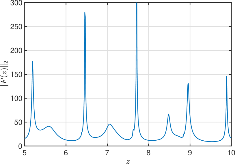
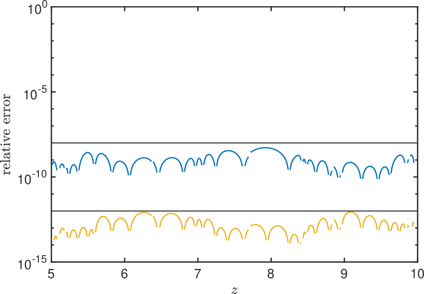
Figure 3: Scattering problem. Left: the Euclidean norm of $\mathbf{f}(z)$ as a function of $z$. Right: the relative error $\|\mathbf{f}(z)-\mathbf{r}^{(d)}(z)\|_{\infty}/\max_{z}\|\mathbf{f}(z)\|_{\infty}$ for the rational approximants $\mathbf{r}^{(d)}(z)$ with $\ell=24$ probing vectors. The dark grey lines indicate the tolerances requested, namely, $10^{-8}$ and $10^{-12}$.

4.4 Boundary element matrices

Our last example is a nonlinear eigenvalue problem that arises from the boundary integral formulation of an elliptic PDE eigenvalue problem [25]. More specifically, we consider the 2D Laplace eigenvalue problem on the Fichera corner from [4, Section 4]. Applying the boundary element method (BEM) to this problem results in a matrix-valued function $F\colon\mathbb{C}\to\mathbb{C}^{n\times n}$ that is dense and not available in split form. Also, the entries of $F(z)$ are expensive to evaluate. Note, however, that hierarchical matrix techniques could be used to significantly accelerate assembly, resulting in a representation of $F(z)$ that allows for fast matrix-vector products [24]. Usually, the smallest (real) eigenvalues of $F$ are of interest. As the smallest eigenvalue is roughly $6.5$, we consider $z$ in the domain $[5,12]$, which is discretized by 200 equidistant points.

The number of boundary elements determines the size of the matrix $F(z)\in{\mathbb{C}}^{n\times n}$. We present two sets of numerical experiments depending on whether we can store the evaluations $F(z_{i})$ for all sampling points $z_{i}\in\Sigma$ on our machine with 64 GB RAM.

Storage possible

The largest problem size that allows for storing all necessary evaluations of $F$ is $n=384$. The computational results are depicted in Table 8. Like for the scattering problem, we see that larger sketch sizes are needed but sketchAAA remains very fast and accurate. For example, with $\ell=16$ and for a stopping tolerance of 1e-08, sketchAAA is about 220 times faster than set-valued AAA applied to ${\mathrm{vec}}(F(z))$ and achieves comparable accuracy. For a stopping tolerance of 1e-12, sketchAAA is about 350 times faster than set-valued AAA applied to ${\mathrm{vec}}(F(z))$.

In all cases of Table 8, we excluded the 3.2 seconds it took to evaluate $F(z_{i})$ for all $z_{i}\in\Sigma$. Both the set-valued AAA and sketchAAA method require these evaluations.

reltol	$\ell$	time (s.)	degree	error
1e-08	$\infty$	15.147	11.0	1.4e-09
	1	0.023	7.4	1.9e-04
	4	0.030	10.0	1.3e-07
	8	0.045	10.3	2.6e-08
	16	0.067	10.8	5.2e-09
1e-12	$\infty$	21.737	14.0	2.0e-13
	1	0.023	9.1	2.1e-05
	4	0.034	12.9	5.7e-11
	8	0.046	13.3	7.1e-12
	16	0.061	14.0	2.6e-13

Table 8: BEM problem from section 4.4: time to execute sketchAAA given the evaluation of $F$ on $\Sigma$, the degree and relative error in the $\infty$-norm of the resulting sketchAAA approximation $R^{(d)}$ for 10 random realizations. The value $\ell=\infty$ indicates no sketching and corresponds to SV-AAA applied to ${\mathrm{vec}}(F(z))$. For $\ell>0$, full (non-tensorized) sketches where used.

Storage not possible

For larger problems, $F(z_{i})$ is evaluated when needed but never stored for all $z_{i}\in\Sigma$. In Table 9 we list the results for tolerance $10^{-12}$. The degree and time for dense and tensor sketches are very similar and we therefore only show the results for tensor sketches. The errors for both the full and tensorized sketches are shown, even though they are also similar.

We observe that the runtime of the whole algorithm is considerably higher. As expected it grows with $N$. The degree and the error, on the other hand, remain very similar to those for the small problem and the main conclusion remains: for $\ell=1$ the sketchAAA approximation is not accurate, but already for $\ell=4$ we obtain satisfactory results at the expense of only slightly increasing the runtime. In addition, even taking a large number of sketches $\ell=24$ is computationally feasible whereas applying SV-AAA to the original problem is far beyond what is possible on a normal desktop.

size $n$	$\ell$	time (s.)	degree	error	error∗
384	1	26.134	9.4	1.2e-05	2.1e-05
	4	30.490	12.9	4.1e-11	5.7e-11
	8	31.132	13.4	8.7e-12	6.8e-12
	16	31.968	14.0	2.8e-13	2.6e-13
	24	32.017	14.0	2.2e-13	2.2e-13
864	1	130.172	9.1	7.6e-06	1.4e-05
	4	154.802	13.0	7.6e-11	5.0e-11
	8	159.993	13.8	6.6e-12	1.3e-11
	16	161.689	14.0	9.0e-13	7.5e-13
	24	161.614	14.0	6.9e-13	4.9e-13
1536	1	412.007	9.0	1.4e-05	8.6e-06
	4	489.553	12.9	5.5e-10	7.8e-11
	8	507.866	13.8	1.2e-11	1.5e-11
	16	512.706	14.0	1.4e-12	1.5e-12
	24	512.984	14.0	9.3e-13	1.2e-12
2400	1	1010.040	9.1	6.6e-06	1.5e-05
	4	1194.473	12.9	2.4e-10	1.3e-10
	8	1244.731	13.9	6.7e-12	1.2e-11
	16	1250.988	14.0	1.5e-12	1.8e-12
	24	1252.066	14.0	1.5e-12	1.4e-12

Table 9: BEM problem from section 4.4: time to run sketchAAA where $F(z_{i})$ is evaluated on the fly, and the average degree and relative error in the $\infty$-norm of the resulting AAA approximation $R^{(d)}$ for 10 random realizations. All numbers correspond to tensorized sketches except the numbers in the column error^∗ which reports the error obtained with full (non-tensorized) sketches. In all cases the tolerance reltol was $10^{-12}$.

5 Conclusions

We have presented and analyzed a new randomized sketching approach which allows for the fast and efficient rational approximation of large-scale vector- and matrix-valued functions. Compared to the original surrogate-AAA approach in [5], our method sketchAAA reliably achieves high approximation accuracy by using multiple (tensorized or non-tensorized) probing vectors. We have demonstrated the method’s performance on a number of nonlinear functions arising in several applications. Compared to the set-valued AAA method from [14], our method works efficiently in the case when the split form of the function to approximate has a large number of terms, and even when the problem is only accessible via function evaluations. We believe that sketchAAA is the first rational approximation method that combines these advantages.

While our focus was on AAA and NLEVPs, let us highlight once more that our sketching approach is not limited to such settings. In principle, any linear (e.g., polynomial or fixed-denominator rational) approximation scheme applied to a large-scale vector-valued function can be accelerated by this approach. For example, current efforts are underway to develop a sketched RKFIT method [1] as a replacement of the surrogate-AAA eigensolver in the MATLAB Rational Krylov Toolbox (the latter of which is currently using only $\ell=1$ sketching vector).

We believe that there are a number of interesting research directions arising from this work. This includes a possible extension to the multivariate case. A multivariate p-AAA algorithm has recently been proposed in [21] but it is not immediately clear whether the sketching idea pursued here can be extended to this algorithm. Another potential improvement of sketchAAA in the case of many sampling points is to replace the SVDs for the least-squares problems (6) by another sketching-based least squares solver such as [22], similarly to what has been done in [16]. Finally, we hope that the analysis provided in this paper might shed some more light onto the accuracy of contour integral-based solvers for linear eigenvalue problems $A\mathbf{x}=\lambda\mathbf{x}$. These methods can be viewed as pole finders for the resolvent $(A-zI)^{-1}$ after random tensorized probing of the form $\mathbf{u}^{T}(A-zI)^{-1}\mathbf{v}$.

References

- [1] M. Berljafa and S. Güttel, The RKFIT algorithm for nonlinear rational approximation, SIAM J. Sci. Comput., 39 (2017), pp. A2049–A2071.
- [2] T. Betcke, N. J. Higham, V. Mehrmann, C. Schröder, and F. Tisseur, NLEVP: A collection of nonlinear eigenvalue problems, ACM Trans. Math. Software, 39 (2013), pp. 1–28.
- [3] Z. Bujanović and D. Kressner, Norm and trace estimation with random rank-one vectors, SIAM J. Matrix Anal. Appl., 42 (2021), pp. 202–223.
- [4] C. Effenberger and D. Kressner, Chebyshev interpolation for nonlinear eigenvalue problems, BIT, 52 (2012), pp. 933–951.
- [5] S. Elsworth and S. Güttel, Conversions between barycentric, RKFUN, and Newton representations of rational interpolants, Linear Algebra Appl., 576 (2019), pp. 246–257.
- [6] I. V. Gosea and S. Güttel, Algorithms for the rational approximation of matrix-valued functions, SIAM J. Sci. Comput., 43 (2021), pp. A3033–A3054.
- [7] S. Gratton and D. Titley-Peloquin, Improved bounds for small-sample estimation, SIAM J. Matrix Anal. Appl., 39 (2018), pp. 922–931.
- [8] T. Gudmundsson, C. S. Kenney, and A. J. Laub, Small-sample statistical estimates for matrix norms, SIAM J. Matrix Anal. Appl., 16 (1995), pp. 776–792.
- [9] B. Gustavsen and A. Semlyen, Rational approximation of frequency domain responses by vector fitting, IEEE Trans. Power Del., 14 (1999), pp. 1052–1061.
- [10] S. Güttel and F. Tisseur, The nonlinear eigenvalue problem, Acta Numer., 26 (2017), pp. 1–94.
- [11] W. Hackbusch, Tensor Spaces and Numerical Tensor Calculus, vol. 56 of Springer Series in Computational Mathematics, Springer, Cham, second ed., 2019.
- [12] N. J. Higham, G. M. Negri Porzio, and F. Tisseur, An Updated Set of Nonlinear Eigenvalue Problems. http://eprints.maths.manchester.ac.uk/2699/, Mar. 2019.
- [13] A. Hochman, FastAAA: A fast rational-function fitter, in 26th IEEE Conference on Electrical Performance of Electronic Packaging and Systems (EPEPS), IEEE, 2017, pp. 1–3.
- [14] P. Lietaert, K. Meerbergen, J. Pérez, and B. Vandereycken, Automatic rational approximation and linearization of nonlinear eigenvalue problems, IMA J. Numer. Anal., (2021).
- [15] A. Mayo and A. Antoulas, A framework for the solution of the generalized realization problem, Linear Algebra Appl., 425 (2007), pp. 634–662.
- [16] Y. Nakatsukasa and T. Park, A fast randomized algorithm for computing the null space, arXiv preprint arXiv:2206.00975, (2022).
- [17] Y. Nakatsukasa, O. Sète, and L. N. Trefethen, The AAA algorithm for rational approximation, SIAM J. Sci. Comput., 40 (2018), pp. A1494–A1522.
- [18] G. M. Negri Porzio, S. Güttel, and F. Tisseur, Robust rational approximations of nonlinear eigenvalue problems, SIAM J. Sci. Comput., 44 (2022), pp. A2439–A2463.
- [19] D. Pradovera, Interpolatory rational model order reduction of parametric problems lacking uniform inf-sup stability, SIAM J. Numer. Anal., 58 (2020), pp. 2265–2293.
- [20] , Model order reduction based on functional rational approximants for parametric PDEs with meromorphic structure, PhD thesis, EPFL, 2021.
- [21] A. C. Rodriguez and S. Gugercin, The p-AAA algorithm for data driven modeling of parametric dynamical systems, tech. rep., arXiv preprint arXiv:2003.06536, 2020.
- [22] V. Rokhlin and M. Tygert, A fast randomized algorithm for overdetermined linear least-squares regression, Proc. Natl. Acad. Sci. USA, 105 (2008), pp. 13212–13217.
- [23] F. Roosta-Khorasani, G. J. Székely, and U. M. Ascher, Assessing stochastic algorithms for large scale nonlinear least squares problems using extremal probabilities of linear combinations of gamma random variables, SIAM/ASA J. Uncertain. Quantif., 3 (2015), pp. 61–90.
- [24] S. A. Sauter and C. Schwab, Boundary Element Methods, Springer, 2011.
- [25] O. Steinbach and G. Unger, A boundary element method for the Dirichlet eigenvalue problem of the Laplace operator, Numer. Math., 113 (2009), pp. 281–298.