Linear Interpolation In Parameter Space is Good Enough for Fine-Tuned Language Models

Abstract

The simplest way to obtain continuous interpolation between two points in high dimensional space is to draw a line between them. While previous works focused on the general connectivity between model parameters, we explored linear interpolation for parameters of pre-trained models after fine-tuning. Surprisingly, we could perform linear interpolation without a performance drop in intermediate points for fine-tuned models. For controllable text generation, such interpolation could be seen as moving a model towards or against the desired text attribute (e.g., positive sentiment), which could be used as grounds for further methods for controllable text generation without inference speed overhead.

1 Introduction

Currently, large pre-trained transformer models can be considered a default choice for various NLP tasks. Training these models is a complex non-linear task that is usually performed by feeding the model a large training corpus and training it in a self-supervised manner (Devlin et al., 2019; Lan et al., 2020; Liu et al., 2019; Radford et al., 2019). Weights obtained by this process are used either for standard fine-tuning or other methods that can be considered more effective in terms of trainable parameters (Liu et al., 2021c, b; Li and Liang, 2021; Lester et al., 2021; Houlsby et al., 2019; Hu et al., 2021).

Since initialization using pre-trained parameters is crucial for the final model’s performance, it is fascinating to observe the changes in parameters during the fine-tuning process on downstream tasks.

While recent works (Goodfellow et al. 2014, Lucas et al. 2021) explored changes in parameter space during training, there is still little known about the details of this process, specifically for model fine-tuning. In our work, we are exploring properties of the fine-tuned language models obtained by linear interpolation.

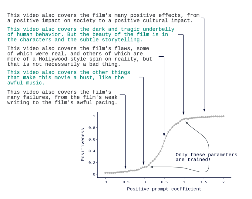
Figure 1: We experimented with linear interpolation for fine-tuned Language Models. We observed that we could fine-tune a pre-trained model on two domains (e.g., positive and negative movie reviews) and interpolate between trained weights without loss in perplexity in between these models. Furthermore, we could expand interpolation beyond trained models and get more positive or negative models than fine-tuned ones.

Surprisingly, we observed compelling evidence of the linearity of some parameter subspace of pre-trained models. The formula behind interpolation is simply

$$\alpha\theta^{-}+(1-\alpha)\theta^{+},$$

where $\alpha\in\mathbb{R}$ is an interpolation weight, and $\theta^{-}$, $\theta^{+}$ are model parameters. If both $\theta^{-}$ and $\theta^{+}$ are fine-tuned LMs (e.g., with negative and positive sentiment generations), the model parameters obtained by applying this formula are well-behaved in terms of perplexity. Therefore, the probability of positive sentiment occurring in the generated text is smoothly growing with the interpolation coefficient weight.

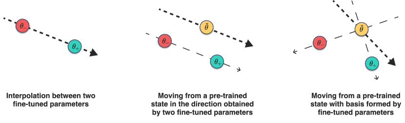
Figure 2: Schematic overview of interpolation schemas used in our experiments. (Left) Interpolation between two fine-tuned model parameters $g_{1}(\alpha)$. (Center) Direction obtained by two fine-tuned model parameters used to move pre-trained model parameters to obtain $g_{2}(\alpha)$. (Right) Two directions formed by fine-tuned parameters and pre-trained weight define the basis used to define the direction in which the pre-trained parameter is moved to get $g_{3}(\alpha,\beta)$. See Section 3.1 for more details.

We investigated the reasons for this phenomenon and found that the same initialization from pre-trained models is crucial for the linear properties.

Utilizing the parameter space is interesting in terms of theoretical results and insights, but what is more important is that it can be used for practical tasks. E.g., linear interpolation makes it possible to apply two attributes in a condition at the same time, or improve attribute presence with desired weight without any computational overhead.

2 Related Work

Goodfellow et al. 2014 found that the loss landscape during interpolation between initial weights and weights after training has no significant peaks and decreases monotonically during interpolation. This is interesting since training is a complex non-linear task, and model weights tend to fall into a local optima point after training is complete. Continuing this line of research Lucas et al. 2021 found a link between batch normalization Ioffe and Szegedy (2015) and linearity of the logits’ path during training.

These observations raise a question about how we can interpolate between two local optima without a loss in quality. Frankle et al. 2020 discovered evidence showing that finding a winning ticket Frankle and Carbin (2018) during iterative pruning is closely connected to finding linear connectivity between optimal points in a weight space. In addition, Frankle et al. 2020 proposed the Loss Barrier metric for evaluating the connectivity between parameters of two models.

Entezari et al. 2021 explored the impact of the width and depth of networks on their connectivity. Their findings showed that the wider the network is, the lower its loss barrier. Meanwhile, the deeper the network is, the higher its barrier value. Furthermore, Entezari et al. 2021 proposed a conjecture about weight permutations and solutions obtained by gradient descent. More precisely, most SGD solutions belong to a set $S$, whose elements can be permuted in such a way that there is no barrier to the linear interpolation between any two permuted elements in $S$. Ainsworth et al. 2022 proposed several methods for sufficient permutation in order to reduce the loss barrier.

To further explore why a zero loss barrier is possible, the Lazy Training theory Chizat et al. (2018) can be used. I.e., if a neural network has sufficient width, the weights’ changes during training are small enough to use the Taylor series expansion for the layer outputs. Therefore, inside some small neighborhood of the initial point, $\theta^{0}$ in the weight space model can be linearized in terms of the weights $\theta$.

3 Understanding Pre-Trained Weights’ Parameter Space

Having a model pre-trained on some general task (e.g., Language Modeling) $\theta^{0}\in\mathbb{R}^{|\theta|}$, it is conventional to initialize a new model with $\theta^{0}$ when solving a downstream task. For example, GPT-2 could be used as $\theta^{0}$ when training an LM on some specific domain of data (e.g., movie reviews). Doing so makes it possible to obtain faster convergence of training procedures and better results than training from scratch since $\theta^{0}$ is usually trained with a larger dataset than those available for downstream tasks.

While many works explore the parameter space of models trained from scratch, we are most interested in such a space for fine-tuned models. More specifically, when a model is trained from scratch with different starting points, there is evidence that different $\theta^{0}$ could be obtained. Furthermore, if different random seeds are used to form mini-batches from the training dataset, additional differences could occur in the resulting parameters of trained models.

It is important to note that, if we train a model from a pre-trained state, we eliminate the randomness caused by different starting points of optimization. From such perspective, we should expect the parameter space of fine-tuned models to be simpler than that of models trained from scratch. To explore the limits of this simplicity, we experimented with linear interpolation between weights of fine-tuned models described in the following sections.

3.1 Linear Interpolation

Consider two models with parameters $\theta^{+}\in\mathbb{R}^{|\theta|}$ and $\theta^{-}\in\mathbb{R}^{|\theta|}$. Both $\theta^{+}$ and $\theta^{-}$ are obtained after fine-tuning a pre-trained model $\theta^{0}$. For convenience, let us consider that $\theta^{0}$ is Language Model trained on general domain data (e.g., GPT-2), $\theta_{+}$ and $\theta_{-}$ are Language Models fine-tuned on positive and negative sentiment data (e.g., SST dataset (Socher et al., 2013)). We could linearly interpolate between them as

$$g_{1}(\alpha)=\alpha\theta^{+}+(1-\alpha)\theta^{-},g_{1}:R\to R^{|\theta|}.$$ (1)

We can also rewrite $g_{1}(\alpha)$ differently:

$$g_{1}(\alpha)=\frac{1}{2}(\theta^{+}+\theta^{-})+\frac{1}{2}(2\alpha-1)(\theta^{+}-\theta^{-}),$$ (2)

which could be seen as moving from starting point $\frac{1}{2}(\theta^{+}+\theta^{-})$ in a direction $(\theta^{+}-\theta^{-})$. Expressing interpolation with a starting point such as that in Equation 2 could be considered too verbose. However, it allows us to derive the second possible formulation of interpolation, for which we replace the starting moving point with $\theta_{0}$. To simplify the process even further, we use $\alpha^{\prime}=2\alpha-1$ as an interpolation weight.

$$g_{2}(\alpha^{\prime})=\theta^{0}+\alpha^{\prime}(\theta^{+}-\theta^{-}).$$ (3)

Going even further, we can decompose the $(\theta^{+}-\theta^{-})$ direction into $(\theta^{+}-\theta^{0})$ and $(\theta^{-}-\theta^{0})$, obtaining new parametrization

$$g_{3}(\alpha,\beta)=\theta^{0}+\alpha(\theta^{+}-\theta^{0})+\beta(\theta^{-}-\theta^{0}).$$ (4)

Note that $\alpha+\beta=1$ reparametrizes $g_{1}$ and $\alpha+\beta=0$ reparametrizes $g_{2}$.

We discuss the limits of these reparametrizations in the Experiments section.

3.2 Ensembling

Another way to utilize several models at once is to combine them into an ensemble. While linear interpolation is performed in the weight space, ensembling can be seen as interpolating in the model output space. At every step, language models yield logits $z$ for every token in vocabulary. As proposed in DExperts Liu et al. (2021a), we could use these logits to obtain the final tokens’ probability:

$$P(x_{t}|x_{<t})=\operatorname{softmax(z)},$$

$$z=z^{0}(x_{<t})+\alpha\cdot(z^{+}(x_{<t})-z^{-}(x_{<t}))$$

However, this method requires significant computational time overhead compared to interpolation in the parameter space since it requires evaluating several models to get predictions.

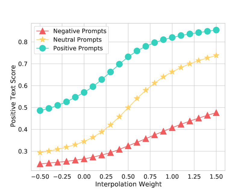
((a))

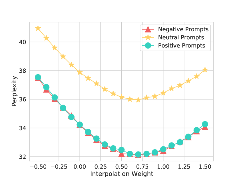
((b))

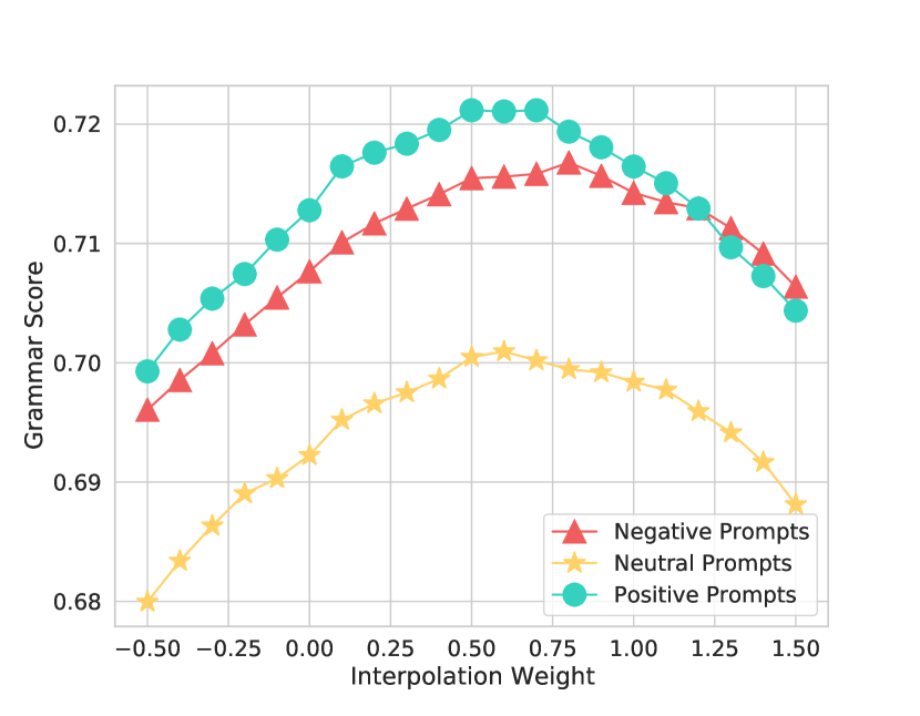
((c))

Figure 3: Interpolation between two models fine-tuned on positive and negative sentiment with $g_{1}(\alpha)$. We report the Mean probability of the positive sentiment (a), the Perplexity of the generated text (b), and the Probability of the grammatically correct text (c) for obtained interpolated models. See Section 4.1 for more details.

4 Experiments

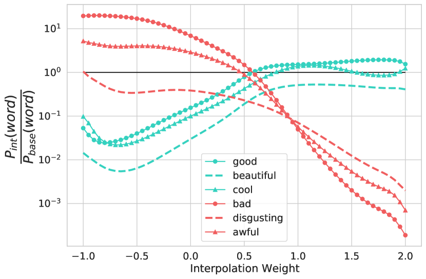
Figure 4: Words’ probability during interpolation with the text prompt "The movie was". Words leading to positive sentiment are plotted in green, and negative in red. While interpolating between $\theta^{-}$ and $\theta^{+}$, probabilities of negative words decrease, and positive ones increase. See Section 4.1 for more details.

4.1 Controllable Text Generation

Controllable text generation can be seen as the simplest way to explore the parameter space of fine-tuned models. The performance of obtained $\theta$ can be quickly evaluated with automatic metrics such as desired attribute probability of generated texts, and text quality can be evaluated by perplexity and grammar correctness.

Following the DExperts Liu et al. (2021a) setup, we took the SST dataset containing texts with labels representing the sentiment of sequences. We constructed a positive sentiment dataset containing texts with labels such as "positive" or "very positive". In addition, we also created a negative dataset with "negative" and "very negative" texts. We then fine-tuned two GPT-2 Large models on the causal language modeling task on these datasets to obtain $\theta^{+}$ and $\theta^{-}$, respectively.

We then evaluated the models obtained by $g_{1}$ and $g_{2}$ (See Equations 1, 3) to understand the limits of linear interpolation for fine-tuned models. To do so, we used the same prompts as DExperts Liu et al. (2021a) for text generation. For every prompt, we generated 25 continuations with their length less or equal to 30 tokens.

We used three metrics to evaluate the generated texts’ sentiment and quality. Positive text scores are evaluated using an external classifier and show the mean probability of positive sentiment in the generated text. Grammar scores are determined by a classifier trained on the CoLA Wang et al. (2018) dataset. To evaluate the texts’ quality, we calculate perplexity using GPT-2 XL.

See Section A.1 of the Appendix for more details on training and evaluation used in these experiments.

See Figure 3 for the results. We found that perplexity with $g_{1}(\alpha)$ remains stable in $\alpha\in[0;1]$, in which we have a zero perplexity barrier. A wider interval of $\alpha$ also shows promising results, where the positive sentiment probability increases with $\alpha>1$. Meanwhile, perplexity and grammar remain stable. Based on this, we can assume that models obtained by simple linear interpolation can still be considered language models. Moreover, the original’s features, such as positive sentiment probability, could be enhanced by $\alpha>1$ (and vice versa). In Section 5, we hypothesise why linear interpolation in the weight space works even in cases of complex non-linear models.

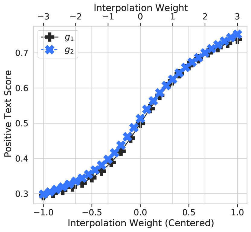
((a))

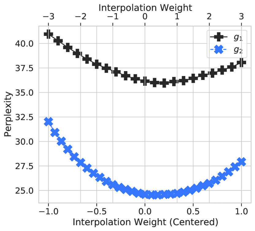
((b))

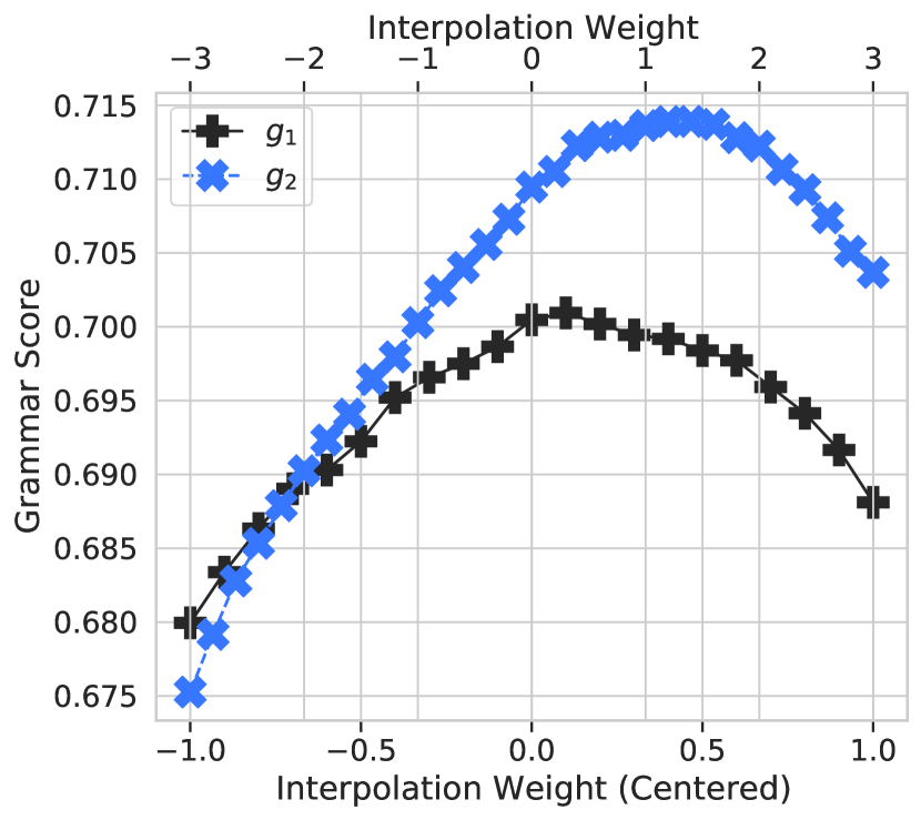
((c))

Figure 5: Comparison of $g_{1}(\alpha)$ and $g_{2}(\alpha)$ interpolations with neutral prompts. We evaluated the positive text score (a), perplexity (b), and Grammar Correctness (c) for interpolated models. Note that these interpolation methods differ in the scale of $\alpha$ (See Section 3.1 for details). Therefore, we used different scales to report these results. $\alpha$ values for $g_{1}(\alpha)$ are shown below the plot, while those for $g_{2}(\alpha)$ are above. While the positiveness of both approaches is comparable, $g_{2}(\alpha)$ obtained better perplexity and grammar correctness through utilizing $\theta^{0}$ parameters. See Section 4.2 for more details.

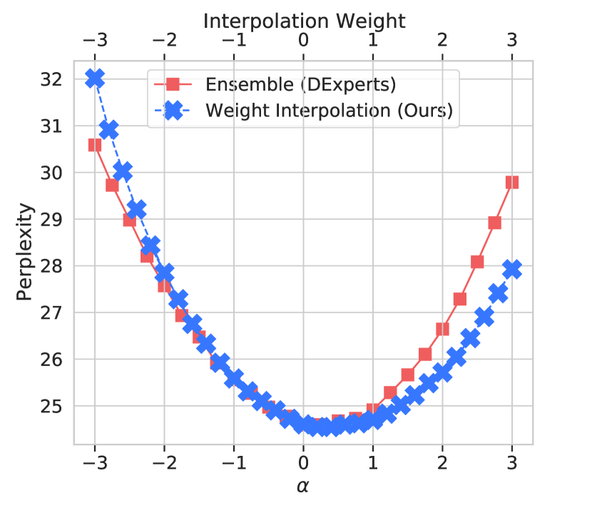
((a))

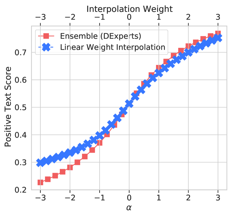
((b))

Figure 6: Perplexity (a) and Positive Text Score (b) with respect to interpolation weight in the logits space (DExperts) and the weight space. Note that the text’s positiveness increases smoothly in booth cases, while perplexity remains low. See Section 4 for more details.

We also measured the next token probability on our "The movie was" prompt using parameters obtained from $g_{1}$ interpolation. See Figure 4 for the results. The probabilities of the words leading to positive sentiment are monotonically increasing, while the probabilities of the negative sentiment words are monotonically decreasing with $\alpha$.

4.2 Which Parametrization Is Best?

In Section 3.1, we discussed different ways to parametrize interpolation and move the model’s weights in the desired direction. However, note that it is not fully clear what the differences are between them. To compare the proposed interpolation schemes, we conducted experiments with the pre-trained model GPT-2 Large as $\theta^{0}$ and Fine-Tuned models from the previous section as $\theta^{+}$ and $\theta^{-}$. Note that parametrization $g_{2}$ takes three models as input.

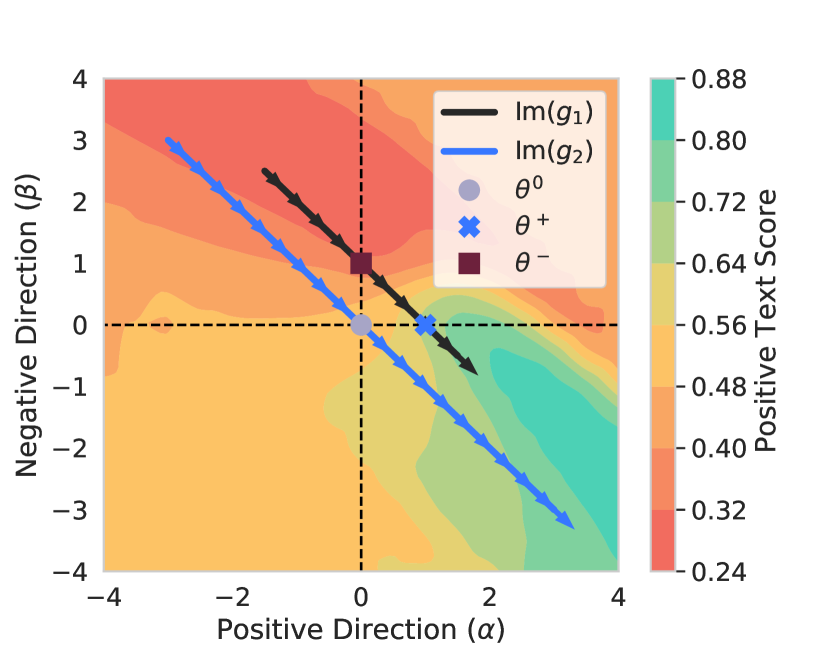
((a))

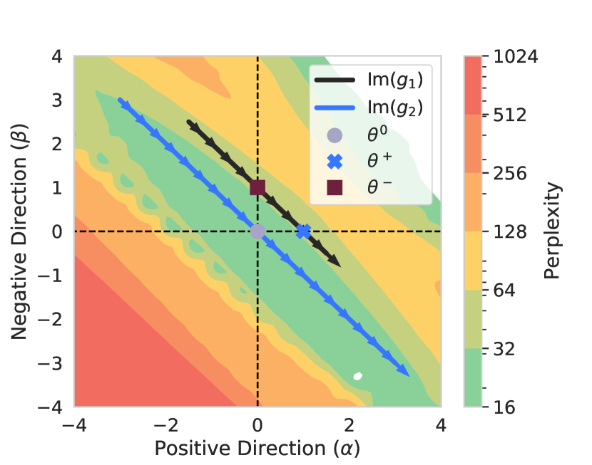
((b))

Figure 7: Postive text score (a) and perplexity (b) for $g_{3}(\alpha,\beta)$ interpolation. Positive text score has a clear growing direction from upper left to lower right. We also found plateau of perplexity near $\alpha=-\beta$ line. See Section 4.3 for more details.

In this subsection, all experiments were conducted with neutral prompts only. See Figure 5 for the results. We observed that $g_{1}(\alpha)$ obtained a positiveness score comparable with $g_{2}(\alpha)$, while the latter showed better perplexity and grammar correctness. However, we would like to note that, in this case, perplexity should not be considered fully representative of the generated texts’ quality. Since $g_{2}(\alpha)$ utilizes $\theta^{0}$, its samplings are more likely to produce texts which would be treated as more probable by GPT-2, while $g_{1}(\alpha)$ has a stronger shift towards movie reviews.

4.3 Interpolation Space

To further analyze the interpolation points, we conduct experiments with interpolation $\theta=g_{3}(\alpha,\beta)$. Note that $g_{3}:\mathbb{R}^{2}\to\mathbb{R}^{|\theta|}$ maps point $(0,1)$ to $g(0,1)=\theta^{0}-\theta^{0}+\theta^{+}-0\cdot(\theta^{-}-\theta^{0})=\theta^{+}$, analogously $(0,0)\to\theta^{0}$ and $(1,0)\to\theta^{-}$. Then we can choose any point in $\mathbb{R}^{2}=\operatorname{dom}g$ and obtain a model $\theta=g(\alpha,\beta)$. We use a 2d uniform grid with values from -4 to +4 and 20 points in every dimension ($G=\{i/2.5\}_{i=-10}^{10}\times\{j/2.5\}_{j=-10}^{10}$) to obtain 400 models, and measure the properties of these models. As a result, we get 400 points of perplexity and a positive sentiment score shown in Figure 7. In addition, we also count the models’ mean negative log-likelihood loss value on a test set of SST positive and negative subsets. See Figure 8 for the results.

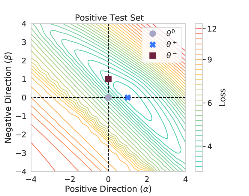
((a))

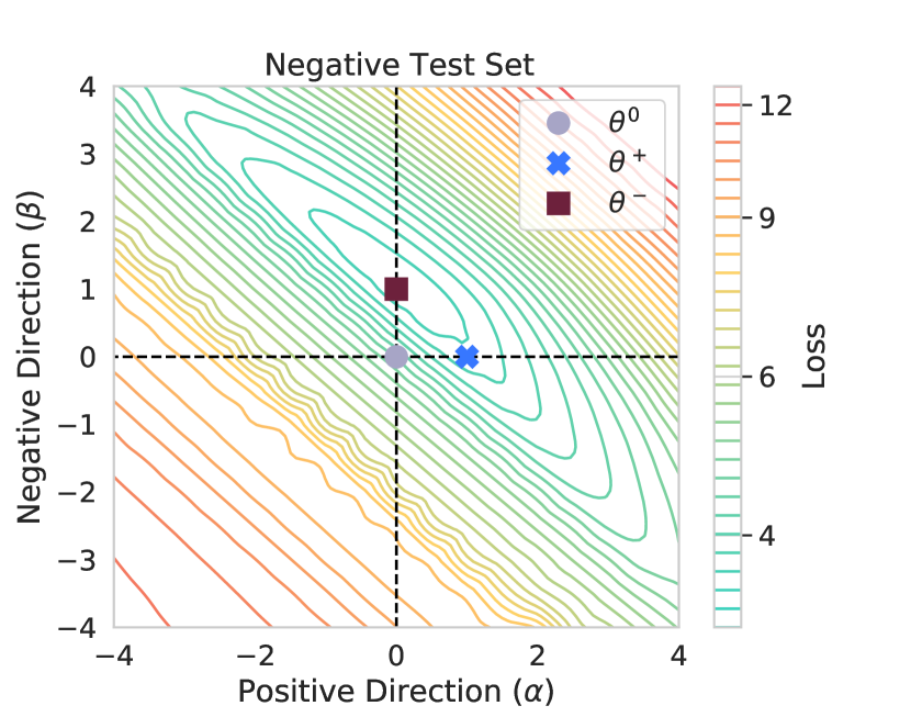
((b))

Figure 8: Positive (a) and negative (b) test set losses for the models obtained by $\theta=g_{3}(\alpha,\beta)$ interpolation. See Section 4.3 for more details.

We found a plateau of perplexity near the $\alpha=-\beta$ line. Furthermore, we also found that the loss values of models near $\alpha=-\beta+1$ (equals to $\theta=g_{2}(\cdot)$ parametrization) are significantly lower. These results can be explained as follows. The first parametrization $\theta=g_{1}(\cdot)$ does not utilize a pre-trained $\theta^{0}$ model. Therefore, the obtained models remain within the SST dataset domain (movie reviews). We can assume that it is because of lower loss on both test subsets. The perplexity of the specific texts is higher due to them becoming biased toward the movie review style. The model we used to measure perplexity (pre-trained GPT-2 XL) is not a domain-specific model and therefore measures information contained in the generated text. As the domain of the generated texts shifted, we observed consistently higher perplexity compared to $\theta=g_{2}(\cdot)$. However, this perplexity remained stable and in a meaningful value below 50. On the other hand, the parametrization $\theta=g_{2}(\cdot)$ did not shift toward the movie reviews domain because of the constant persistence of the $\theta^{0}$ term. Lower perplexity, in this case, did not indicate better quality of the generated texts.

4.4 Interpolation vs. Ensembling

In this section, we compare two methods of utilizing several models for controllable text generation tasks.

As discussed in 3.2, DExperts could be seen as a linear interpolation in the model outputs space.

We generated texts with several values of the $\alpha$ parameter. Then, we used $\theta^{+}$ model as an expert and $\theta^{-}$ model as an anti-expert. We compared this setup with $\theta=g_{2}(\alpha)$ parametrization. The results are presented in Figure 6.

We found that the curves are almost identical for $\alpha\in[0;1]$. Similar results could be obtained if all model backbones were linear. Surprisingly for us, we also discovered that linear interpolation in weight space is highly competitive to ensembling and does not damage the internal knowledge of the model.

5 Results Analysis

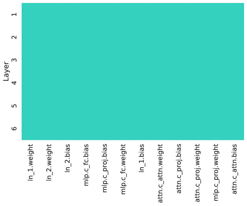
((a))

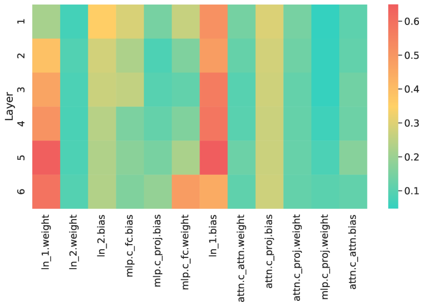
((b))

Figure 9: The norm of the weight difference for $\theta^{+}$ and $\theta^{0}$ (a), as well as DistilGPT-2 trained on C4 Raffel et al. (2020) from scratch and pre-trained DistilGPT-2 (b). Each row represents one layer, and the parameter names can be found on the x-axis ticks. See Section 5.3 for more details.

To explain the results of the above observations, we will now try to establish some intuition on why linear interpolation works so well for pre-trained language models.

5.1 Lazy Training

Lazy training, introduced by Chizat et al. 2018, has a solid connection to linear interpolation in the weight space.

Let us say that we have some function $f(\theta)=R(h(\theta)):\mathbb{R}^{|\theta|}\to\mathbb{R}_{+}$, where $h(\theta):\mathbb{R}^{|\theta|}\to\mathcal{F}$ is our model. Now, let us define a linearized model $\overline{h}(\theta)=h(\theta^{0})-Dh(\theta^{0})(\theta^{0}-\theta)$. $\overline{h}(\theta)$ could be seen as a Taylor’s series expansion to the first order of $h(\theta)$. If we can accurately approximate $h(\theta)$ with $\overline{h}(\theta)$, then $\overline{f}(\theta)=R\left(\overline{h}(\theta)\right)$ becomes a good approximation of $f$ if we are using gradient descent for optimizing $R$.

5.2 Pre-Trained Models Fine-Tuning and Lazy Traing

Chizat et al. 2018 considers function $f$ to be a loss function optimized by gradient descent. In our work, we will talk about a proxy function that can be seen as a differentiable interpolation of the positive text score or other desired attributes for controllable text generation. For example, we can start our optimization process at $\theta^{0}$ and train models $\theta_{+}$ and $\theta_{-}$ using stochastic gradient descent on the NLL target function. We believe that after minimization, some function $f$ (in our case, the probability of positive sentiment in the generated text) will have a lower value on $\theta^{-}$ and a higher value on $\theta^{+}$. In other words, during the training procedure, we are trying to find weights $\theta^{-}$ and $\theta^{+}$ such that $f(\theta^{-})<f(\theta^{0})<f(\theta^{+})$.

Conjecture. Point $\hat{\theta}$ with the lowest value of the loss function $L$, such as NLL, does not imply optimal value of the truly desired $f$ function. In other words, we can find a value of $\theta^{*}$ with $L(\theta^{*})>L(\hat{\theta})$, but $f(\theta^{*})>f(\hat{\theta})$.

Function $f$ can be a composition of other functions such as a weighted sum of grammar scores, desired and present attributes, and perplexity.

Assumption. If the weights $\theta$ obtained after the fine-tuning procedure are close to pre-trained initialization $\theta^{0}$, we can linearize the function $f$ as $\overline{f}(\theta)=f(\theta^{0})+\nabla f(\theta^{0})^{T}(\theta-\theta_{0})$ in some neighbourhood of $\theta^{0}$.

If we then parametrize $\theta$ with the general parametrization $\theta=g_{3}(\alpha,\beta)=\theta^{0}+\alpha(\theta^{+}-\theta^{0})+\beta(\theta^{-}-\theta^{0})$ and pass it to $\overline{f}$, we obtain

$$\overline{f}\circ g(\alpha,\beta)=f(\theta^{0})$$ (5)

$$+\alpha\cdot\nabla f(\theta^{0})^{T}(\theta^{+}-\theta^{0})$$

$$+\beta\cdot\nabla f(\theta^{0})^{T}(\theta^{-}-\theta^{0})$$

$$=\alpha\cdot C^{+}+\beta\cdot C^{-},$$

where $C^{+}$ and $C^{-}$ are constants.

Note that $C^{+}\approx\partial(f\circ g)/\partial\alpha$ and $C^{-}\approx\partial(f\circ g)/\partial\beta$ in some $\theta^{0}$ neighbourhood.

The scheme with linear interpolation works even if $C^{+}$ and $C^{-}$ are not constants, since $C^{+}(\alpha)$ > 0 and $C^{-}(\beta)<0$ is a sufficient condition.

This model clarifies the similarity between DExperts and linear weight interpolation in Figure 6. If Assumption 5.2 holds, then the interpolation between weights will be approximately equal to the interpolation between outputs in a small enough region around $\theta^{0}$

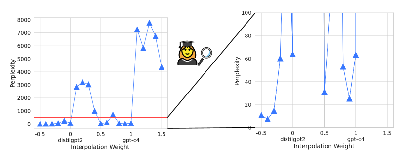
((a))

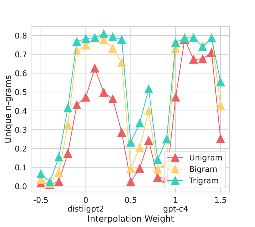
((b))

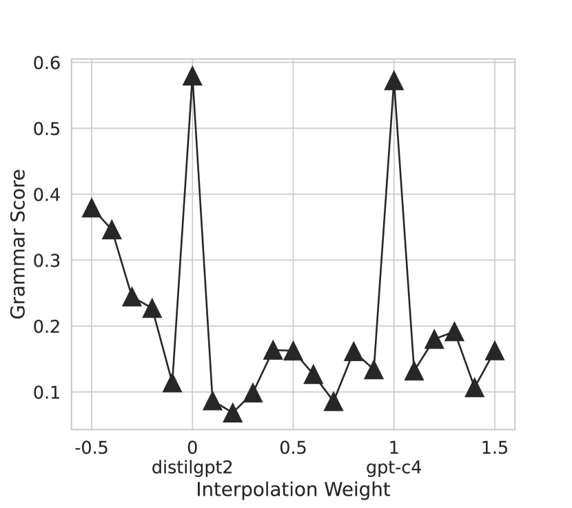
((c))

Figure 10: Linear interpolation between DistilGPT-2 and GPT-C4 weights. We observed that points between original weights performed poorly with increased perplexity (a), the reduced fraction of unique n-grams (b), and grammar score (c). See Section 5.3 for more details.

5.3 Interpolating Between Two Different Decorrelated Language Models

The small difference between weights is the main factor for the above-mentioned theory. We hypothesize that we obtained such a low difference since we performed fine-tuning of the same pre-trained model $\theta^{0}$. To support this, we conduct experiments with two different language models.

For the simplicity of our experiment, we chose a small DistilGPT-2 model Sanh et al. (2019) with 6 hidden layers. We trained a GPT model from scratch on C4 Raffel et al. (2019), namely GPT-C4 with architecture identical to DistilGPT-2. For more details, refer to Section A.2.

Firstly, we measured the norm of the weight differences between two pairs of models.

1. Pre-trained original DistilGPT-2 $\longleftrightarrow$ Fine-tuned original DistilGPT-2 on positive sentiment.

2. Pre-trained original DistilGPT-2 $\longleftrightarrow$ Pre-trained on C4 dataset GPT-C4.

To evaluate the difference between 1-d tensors (biases), we use the scaled $\ell^{2}$-norm:

$$\Delta_{b}=\frac{\lVert b_{1}-b_{2}\rVert}{\sqrt{d}}=\frac{\sqrt{\sum_{i}\left(b_{1}^{i}-b_{2}^{i}\right)^{2}}}{\sqrt{d}}.$$

For matrices with sizes $n\times m$, we use:

$$\Delta_{w}=\frac{\lVert w_{1}-w_{2}\rVert}{\sqrt{n\cdot m}}=\frac{\sqrt{\sum_{i}^{n}\sum_{j}^{m}\left(w_{1}^{ij}-w_{2}^{ij}\right)^{2}}}{\sqrt{n\cdot m}}.$$

Results showed in Figure 9. Note that two comparisons are plotted on the same scale. While the differences between the (a) pair are small, the differences between (b) can be observed.

The second experiment interpolates between two language models: DistilGPT-2 and GPT-C4. See Figure 10 for the results. We found that models obtained at every interpolation step completely forget the knowledge obtained during the training procedure. We additionally estimate the fraction of the distinct n-grams. At every point where perplexity becomes lower than initial values (0 and 1), we observe a significant drop in unique n-grams. The grammar score has two major peaks at points 0 and 1.

Models obtained by interpolating between different pre-trained models were found to fail at the basic language model tasks. This experiment confirms the importance of initializing fine-tuned models in the same way.

6 Conclusion

In our paper, we looked into simple linear weight interpolation between pre-trained and fine-tuned models, and concluded that this method performs surprisingly well. We found that different types of interpolation have different strengths and flaws, which we discuss in detail in the Experiments section. We have researched this phenomenon and provided intuition on why large language models, highly non-linear complex functions, are capable of generating texts with good metrics even after simple linear interpolation.

Appendix A Experiment Details

A.1 Details of Controllable Text Generation Experiments

We fine-tuned two GPT-2 Large models on the SST dataset and ran a hyperparameter search using the grid from Table 1.

Parameter	Values range
Learning rate	[1e-4, 1e-5, 1e-6]
Batch size	[32, 64, 128, 256]
Steps	[500, 1000, 2000]

Table 1: Hyperparameter search ranges used in fine-tuning.

After the training, we proceeded with the best model in terms of perplexity on the corresponding validation sets. The best parameters are reported in Table 2.

Parameter	Positive ($\theta_{+}$)	Negative ($\theta_{-}$)
Learning rate	1e-6	1e-6
Batch size	64	64
Steps	1000	1000

Table 2: Best hyperparameters.

As a Positive Text Score metric, we use outputs of the RoBERTa-base model trained by CardiffNLP Rosenthal et al. (2017). The model outputs consist of three probabilities: negative, neutral and positive sentiment. For the final score, we use the expectation of positive sentiment (see Equation 6).

$$score=0\cdot P(neg)+0.5\cdot P(neutral)+1\cdot P(pos)$$ (6)

For perplexity, we use the GPT-2 XL model and count the perplexity of all generated texts.

We also evaluate the Grammar Score using the RoBERTa-base model fine-tuned on the CoLA dataset by TextAttack Morris et al. (2020). The final score is the mean probability of the text being grammatically correct.

Text generation parameters can be found in Table 3:

Parameter	Value
top-p	0.9
max new tokens	30

Table 3: Parameters used for text generation.

A.2 LM Training Details

We trained a GPT-Like language model on the C4 Raffel et al. (2019) dataset. This model’s architecture is identical to the DistilGPT-2 model Sanh et al. (2019). We used 8x NVidia A100-SXM-80GB GPUs with bf16 mixed precision Burgess et al. (2019). We trained our model for 37K steps with the AdamW Loshchilov and Hutter (2019) optimizer and a cosine scheduler with warmup. Parameters for the training procedure can be found in the table 4. Model was trained until convergence, and the loss dynamic can be found in Figure 11.

Parameter	Value
Max LR	3e-4
Weight decay	0.01
$\beta_{1}$	0.9
$\beta_{2}$	0.95
$\varepsilon$	1e-8
Warmup steps	5000
Effective batch size	1024

Table 4: Parameters used for LM training.

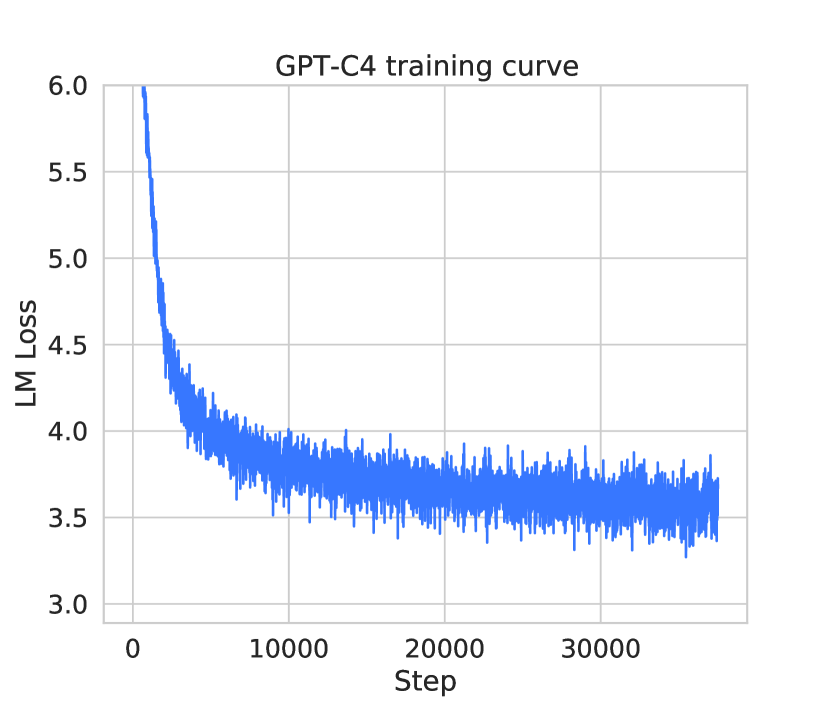
Figure 11: Loss dynamic during LM training.

References

- Ainsworth et al. (2022) Samuel K. Ainsworth, Jonathan Hayase, and Siddhartha Srinivasa. 2022. Git re-basin: Merging models modulo permutation symmetries.
- Burgess et al. (2019) Neil Burgess, Jelena Milanovic, Nigel Stephens, Konstantinos Monachopoulos, and David Mansell. 2019. Bfloat16 processing for neural networks. In 2019 IEEE 26th Symposium on Computer Arithmetic (ARITH), pages 88–91.
- Chizat et al. (2018) Lenaic Chizat, Edouard Oyallon, and Francis Bach. 2018. On lazy training in differentiable programming.
- Devlin et al. (2019) Jacob Devlin, Ming-Wei Chang, Kenton Lee, and Kristina Toutanova. 2019. BERT: Pre-training of deep bidirectional transformers for language understanding. In Proceedings of the 2019 Conference of the North American Chapter of the Association for Computational Linguistics: Human Language Technologies, Volume 1 (Long and Short Papers), pages 4171–4186, Minneapolis, Minnesota. Association for Computational Linguistics.
- Entezari et al. (2021) Rahim Entezari, Hanie Sedghi, Olga Saukh, and Behnam Neyshabur. 2021. The role of permutation invariance in linear mode connectivity of neural networks.
- Frankle and Carbin (2018) Jonathan Frankle and Michael Carbin. 2018. The lottery ticket hypothesis: Training pruned neural networks. CoRR, abs/1803.03635.
- Frankle et al. (2020) Jonathan Frankle, Gintare Karolina Dziugaite, Daniel Roy, and Michael Carbin. 2020. Linear mode connectivity and the lottery ticket hypothesis. In Proceedings of the 37th International Conference on Machine Learning, volume 119 of Proceedings of Machine Learning Research, pages 3259–3269. PMLR.
- Goodfellow et al. (2014) Ian J. Goodfellow, Oriol Vinyals, and Andrew M. Saxe. 2014. Qualitatively characterizing neural network optimization problems.
- Houlsby et al. (2019) Neil Houlsby, Andrei Giurgiu, Stanislaw Jastrzebski, Bruna Morrone, Quentin de Laroussilhe, Andrea Gesmundo, Mona Attariyan, and Sylvain Gelly. 2019. Parameter-efficient transfer learning for nlp. In ICML.
- Hu et al. (2021) Edward J. Hu, Yelong Shen, Phillip Wallis, Zeyuan Allen-Zhu, Yuanzhi Li, Shean Wang, Lu Wang, and Weizhu Chen. 2021. Lora: Low-rank adaptation of large language models.
- Ioffe and Szegedy (2015) Sergey Ioffe and Christian Szegedy. 2015. Batch normalization: Accelerating deep network training by reducing internal covariate shift. In Proceedings of the 32nd International Conference on Machine Learning, volume 37 of Proceedings of Machine Learning Research, pages 448–456, Lille, France. PMLR.
- Lan et al. (2020) Zhenzhong Lan, Mingda Chen, Sebastian Goodman, Kevin Gimpel, Piyush Sharma, and Radu Soricut. 2020. Albert: A lite bert for self-supervised learning of language representations. In International Conference on Learning Representations.
- Lester et al. (2021) Brian Lester, Rami Al-Rfou, and Noah Constant. 2021. The power of scale for parameter-efficient prompt tuning.
- Li and Liang (2021) Xiang Lisa Li and Percy Liang. 2021. Prefix-tuning: Optimizing continuous prompts for generation. In Proceedings of the 59th Annual Meeting of the Association for Computational Linguistics and the 11th International Joint Conference on Natural Language Processing (Volume 1: Long Papers), pages 4582–4597, Online. Association for Computational Linguistics.
- Liu et al. (2021a) Alisa Liu, Maarten Sap, Ximing Lu, Swabha Swayamdipta, Chandra Bhagavatula, Noah A. Smith, and Yejin Choi. 2021a. DExperts: Decoding-time controlled text generation with experts and anti-experts. In Proceedings of the 59th Annual Meeting of the Association for Computational Linguistics and the 11th International Joint Conference on Natural Language Processing (Volume 1: Long Papers), pages 6691–6706, Online. Association for Computational Linguistics.
- Liu et al. (2021b) Xiao Liu, Kaixuan Ji, Yicheng Fu, Zhengxiao Du, Zhilin Yang, and Jie Tang. 2021b. P-tuning v2: Prompt tuning can be comparable to fine-tuning universally across scales and tasks. CoRR, abs/2110.07602.
- Liu et al. (2021c) Xiao Liu, Yanan Zheng, Zhengxiao Du, Ming Ding, Yujie Qian, Zhilin Yang, and Jie Tang. 2021c. Gpt understands, too. arXiv:2103.10385.
- Liu et al. (2019) Yinhan Liu, Myle Ott, Naman Goyal, Jingfei Du, Mandar Joshi, Danqi Chen, Omer Levy, Mike Lewis, Luke Zettlemoyer, and Veselin Stoyanov. 2019. Roberta: A robustly optimized bert pretraining approach. Cite arxiv:1907.11692.
- Loshchilov and Hutter (2019) Ilya Loshchilov and Frank Hutter. 2019. Decoupled weight decay regularization.
- Lucas et al. (2021) James Lucas, Juhan Bae, Michael R. Zhang, Stanislav Fort, Richard Zemel, and Roger Grosse. 2021. Analyzing monotonic linear interpolation in neural network loss landscapes.
- Morris et al. (2020) John Morris, Eli Lifland, Jin Yong Yoo, Jake Grigsby, Di Jin, and Yanjun Qi. 2020. Textattack: A framework for adversarial attacks, data augmentation, and adversarial training in nlp. In Proceedings of the 2020 Conference on Empirical Methods in Natural Language Processing: System Demonstrations, pages 119–126.
- Radford et al. (2019) Alec Radford, Jeff Wu, Rewon Child, David Luan, Dario Amodei, and Ilya Sutskever. 2019. Language models are unsupervised multitask learners.
- Raffel et al. (2019) Colin Raffel, Noam Shazeer, Adam Roberts, Katherine Lee, Sharan Narang, Michael Matena, Yanqi Zhou, Wei Li, and Peter J. Liu. 2019. Exploring the limits of transfer learning with a unified text-to-text transformer. arXiv e-prints.
- Raffel et al. (2020) Colin Raffel, Noam Shazeer, Adam Roberts, Katherine Lee, Sharan Narang, Michael Matena, Yanqi Zhou, Wei Li, and Peter J. Liu. 2020. Exploring the limits of transfer learning with a unified text-to-text transformer. Journal of Machine Learning Research, 21(140):1–67.
- Rosenthal et al. (2017) Sara Rosenthal, Noura Farra, and Preslav Nakov. 2017. Semeval-2017 task 4: Sentiment analysis in twitter. In Proceedings of the 11th international workshop on semantic evaluation (SemEval-2017), pages 502–518.
- Sanh et al. (2019) Victor Sanh, Lysandre Debut, Julien Chaumond, and Thomas Wolf. 2019. Distilbert, a distilled version of bert: smaller, faster, cheaper and lighter. In NeurIPS EMC Workshop.
- Socher et al. (2013) Richard Socher, Alex Perelygin, Jean Wu, Jason Chuang, Christopher D. Manning, Andrew Ng, and Christopher Potts. 2013. Recursive deep models for semantic compositionality over a sentiment treebank. In Proceedings of the 2013 Conference on Empirical Methods in Natural Language Processing, pages 1631–1642, Seattle, Washington, USA. Association for Computational Linguistics.
- Wang et al. (2018) Alex Wang, Amapreet Singh, Julian Michael, Felix Hill, Omer Levy, and Samuel R. Bowman. 2018. Glue: A multi-task benchmark and analysis platform for natural language understanding. Cite arxiv:1804.07461Comment: https://gluebenchmark.com/.