Ultrasound Detection of Subquadricipital Recess Distension

Abstract

Joint bleeding is a common condition for people with hemophilia and, if untreated, can result in hemophilic arthropathy. Ultrasound imaging has recently emerged as an effective tool to diagnose joint recess distension caused by joint bleeding. However, no computer-aided diagnosis tool exists to support the practitioner in the diagnosis process. This paper addresses the problem of automatically detecting the recess and assessing whether it is distended in knee ultrasound images collected in patients with hemophilia. After framing the problem, we propose two different approaches: the first one adopts a one-stage object detection algorithm, while the second one is a multi-task approach with a classification and a detection branch. The experimental evaluation, conducted with $483$ annotated images, shows that the solution based on object detection alone has a balanced accuracy score of $0.74$ with a mean IoU value of $0.66$, while the multi-task approach has a higher balanced accuracy value ($0.78$) at the cost of a slightly lower mean IoU value.

Keywords multi-task learning  $\cdot$ clinical decision support  $\cdot$ ecography  $\cdot$ hemarthrosis

1 Introduction

Hemophilia is a hereditary blood coagulation disorder that results in an increased risk of bleeding, due to trauma or spontaneously, which worsens with the severity of the disease. Bleedings can frequently occur also inside joints (mostly ankles, knees and elbows) and muscles, which together account for around $80\%$ of the bleeding events in patients with Hemophilia [1, 2]. Joint bleeding causes joint recess distension which, if recurrent, can result in synovial hyperplasia, osteochondral damage, and hemophilic arthropathy [3]. Thus, it is essential to promptly recognize joint recess distension.

Physical examination may not be sufficient to diagnose joint recess distension, since in the early stage it can be asymptomatic [4]. Magnetic Resonance Imagining (MRI) is generally considered the gold standard tool for precise evaluation of joints but it is not practical for regular follow-up of patients with haemophilia due to the high costs, limited availability and long examination times [4]. An alternative solution is ultrasound (US) imaging [5] that, contrary to MRI, has a low cost, short examining time and it is widely accessible [6]. Hemophilia Early Arthropathy Detection with UltraSound (HEAD-US) is a standardized protocol designed to guide the practitioner in acquiring relevant US images and interpreting them for the diagnosis of joint recess distension in the $6$ most commonly affected joints [7].

Computer aided diagnosis (CAD) systems can improve detection accuracy [8] and reduce the image reading time required by the practitioners [9]. The potential effectiveness of US-based CAD systems to support the diagnosis of joint distension in people with hemophilia is suggested by recent studies that focus in identifying joint effusions related to injuries [10].

In this work, we formulate the research problem of supporting the physicians in diagnosing joint recess distension in patients with hemophilia using a CAD system. The problem consists of detecting the joint recess inside US images and classifying it as Distended or Non-distended. Specifically, we focus on the main joint recess of the knee, also called SubQuadricipital Recess (SQR). We consider the SQR longitudinal scan, which is one of the three scans specified in HEAD-US protocol for this joint [7]. One prior work addresses the problem of detecting SQR distension in pediatric patients with hemophilia [11], but specific details about the methodology and the evaluation are not reported.

Besides formulating the research problem, we also propose two approaches to address it. The first one, called the Detection approach, adopts state-of-the-art object detection to find Distended or Non-distended SQRs inside the US image and returns the detection having the highest confidence. The second solution, called the Multi-task approach uses a multi-task learning process, with the aim of simultaneously detecting the SQR inside the US image and classifying it as Distended or Non-distended.

The experiments, conducted on a dataset of images we collected and annotated from $200$ adults subjects with hemophilia, reveal that the Multi-task approach improves over the Detection approach in terms of classification accuracy. Indeed, the Balanced Accuracy (BA) is $0.78$ with the Multi-task approach and $0.74$ with the Detection approach. In particular, sensitivity improves from $0,52$ with the Detection approach to $0,64$ with the Multi-task approach. Instead, for what concerns the detection accuracy, the Detection approach has slightly better performance than the Multi-task approach: the average Intersection over Union (IoU) is $0.66$ for the Detection approach and $0.63$ for the Multi-task approach.

To sum up, the novel contributions of this paper are the following:

• We formulate the problem of detecting and classifying distensions in SQR from US images.

• We propose two solutions to tackle this problem.

• We evaluate and compare the proposed solutions on a dataset collected from $200$ patients.

2 Problem formulation

In this research, we address the problem of the automated detection of the subquadricipital recess (SQR) and its classification as Distended or Non-distended.

2.1 Ultrasound images

Ultrasound (US) [12] is a very popular medical imaging technique. It is portable, safe and affordable and therefore commonly used in healthcare [13]. However, some limitations of this technique are the high dependence on the operator expertise level and possible noisiness of the acquired images [4].

US imaging uses sound waves at high frequencies. The reflections of the signal are then measured to represent the image. This technique can produce images with a high spatial resolution of the internal structures of the body, like tendons, bones, blood, and muscles [5]. The images are represented in grayscale, where each pixel value describes the density of the material the signal encounters. Light areas represent echogenic tissues (i.e., that reflect sound waves) like bones, while dark areas represent anechogenic (i.e., that do not reflect sound) structures such as liquids. Another effect to take into account is that echogenic tissues, such as bone, shield the signal that is unable to travel through them, thus making it impossible to detect anything below them. An example is shown in Figure 1: the patella is clearly distinguishable in light color (see the red box) while the area below it is almost completely black.

2.2 Subquadricipital Recess longitudinal scan

We focus on one of the three scans of the knee joint specified in HEAD-US protocol for the collection and diagnosis of joint recess distension in patients with hemophilia [7]: the SQR longitudinal scan. This scan is used to assess SQR distension and contains different characterizing elements (see Figure 1):

• The femur (blue box) usually appears as a light thick line, approximately horizontal, starting from the left side of the image and extending towards the right, often in the lower half of the image.

• The patella (red box) usually appears as a curved light line, positioned at the right border of the image, often in the top half and not entirely captured. The tendons (horizontal and parallel darker lines) can be seen on its left.

• The SQR (green box) often contains at least a small quantity of liquid and hence it is dark. In some cases, the joint recess membrane can be visible in grey. The joint recess is positioned between the femur and the patella. Its size and shape vary depending on many factors including whether it is distended or not, as explained below.

Figure 1b shows how the probe must be positioned during the acquisition of the SQR longitudinal scan. In the figure, the yellow box is the area that is captured by the US image shown in Figure 1a, while the green box is the SQR. To correctly acquire this type of image, the knee has to be bent at 30^∘. The probe must be positioned right at the beginning of the patella and moved horizontally to identify the correct key features previously described.

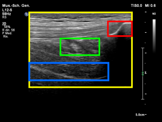
(a) Example of SQR longitudinal scan

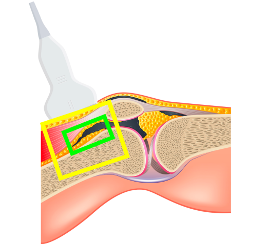
(b) Probe positioning

Figure 1: Image acquisition

2.3 Detection and classification of SQR distension

A joint recess can be distended due to three main reasons: it is filled with synovial liquid, it is filled with blood (a condition known as hemarthrosis), and its membrane is thicker due to an inflammation known as synovitis. When the SQR is distended, it appears thicker on the US image. In some cases this can be clearly visible because the joint recess appears as a large dark area. Figure 2 shows three examples of the longitudinal SQR scan. In Figure 2a the SQR is the dark area shown in the green box. In this case the SQR is thin, hence it is not distended. Vice versa, in Figure 2b the SQR is much thicker, indicating that it is distended. While Figure 2a and 2b show two characteristic examples with stark differences, there are borderline cases where the SQR appears slightly enlarged but it is not distended (see Figure 2c) or it is very slightly distended.

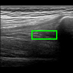
(a) Non-distended SQR

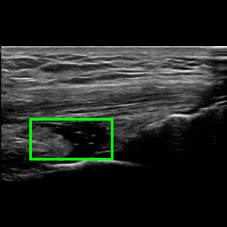
(b) Distended SQR

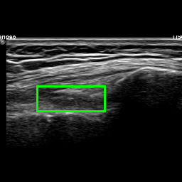
(c) Borderline Non-distended SQR

Figure 2: Examples of longitudinal SQR scans

An analysis, conducted with physicians from the Angelo Bianchi Bonomi Hemophilia and Thrombosis Center (two of which are also authors of this paper), revealed the need for a computer aided tool (CAD) supporting the physician in diagnosing SQR distension. The tool can be used as a part of a protocol for the early diagnosis of hemarthrosis, which is particularly relevant for hemophilic patients [14, 4]. Indeed, directly identifying hemarthrosis in US images is particularly challenging as it requires to distinguish blood from synovial fluid and blood clots from synovial hyperplasia, which appear very similar. To support the physician during the diagnosis, the CAD tool should identify the position of the SQR inside the specified US scan and classify it as Distended or Non-distended.

3 Related work

3.1 US-based CAD systems

Machine Learning (ML) techniques using medical imaging data have been investigated to support physicians in diagnosing various conditions [15]. In particular, Ultrasound (US) [12] is a very popular medical imaging technique, often used also as a data source for Computer-Aided Diagnosis (CAD) systems [16, 13]. Indeed, despite its high dependence on the operator expertise level and possible noisiness of the acquired images [4], US imaging is easily accessible, safe and affordable and therefore commonly used in healthcare [13].

In this problem domain, Convolutional Neural Networks (CNNs) are the most frequently used ML architectures, due to their ability to extract discriminative features from image data [17, 18, 19, 20]. However, the development of such systems is often limited by the scarcity of available labeled data for the training of the ML models. To mitigate this issue, in the literature, transfer learning [21, 22] and generative data augmentation approaches [23, 24] have been proposed.

Classification approaches

One commonly used ML approach in US CAD systems is the direct classification of the images collected by medical experts [25, 26]. Indeed, different studies adopted deep learning classification approaches to identify various pathologies such as tumors in breast ultrasound [27, 28, 29], liver pathologies [30, 31], thyroid nodules [32, 33], and others [19].

Segmentation and detection approaches

Detection and segmentation techniques designed to extract Regions of Interest (ROI) in US images are also common. For example, one solution extracts a ROI of the femural carthilage from US images using segmentation [34]. Other approaches rely on object detection architectures to detect multiple ROIs within a US image for example to detect and classify breast lesions [35] or to detect different types of diseases in several organs [36]. Another example is SonoNet [37], a real-time detection network that identifies fetal standard scan planes in ultrasound 2D images.

Multi-task learning approaches

Previous works have explored the multi-task combination of classification and detection for non-US medical images [38, 39, 40, 41, 42]. However, works exploring multi-task learning on US images are only a few. Gong et al. propose an approach for multi-task localization of the thyroid gland and the detection of nodules within that region, using a shared backbone network which is divided into two different decoders for the two tasks [43]. Zhang et al. adopt a multi-task learning algorithm to segment and classify cancer in Breast US images. They propose to use DenseNet121 as backbone, followed by a decoder branch with layers connected by attention-gated (AG) units to segment the images [44]. The second branch performs a classification task that takes in input the features extracted by the encoder. We are not aware of multi-task learning algorithms adopted to address the problem of joint recess distension detection, and more generally we found no prior works proposing multi-task networks to analyze muskoskeletal US images.

3.2 Joint recess distension detection approaches

US images are commonly used for joint assessment and detection of joint recess distension in hemofilic patients. For this task, HEAD-US [7] is a standardized protocol to support physicians in acquiring US images of commonly affected joints and formulating a diagnosis.

Two solutions have been proposed in the literature to automatically detect and classify joint recess distension but not focusing on patients with hemophilia, like in our contribution. The former focuses on the shoulder joint [45], proposing the use of two CNNs to extract the ROI for Bicipital peritendinous effusions: the VGG-16 [18] network is used for feature extraction, and a second CNN is used to classify the distension in three classes (i.e., mild, moderate, and severe). The latter contribution considers the knee joints [10] and uses segmentation techniques to classify different pathologies inside US images, including joint recess distension due to synovial thickening.

A recent abstract paper [11] considers US images of patients with hemophila and addresses the problem of classifying distended and not-distended knee recesses. However, that prior work does not describe the methodology used for the classification, and it does not detect the joint recess ROI.

4 Methodology

We propose two solutions for the problem defined in Section 2. The first solution, which we name Detection approach, is described in Section 4.1. It is based on a state-of-the-art detection technique, adopted to solve both the detection and the classification problems. The second solution, which we call Multi-task approach (see Section 4.2), is a multi-task network with a branch that solves the detection problem and another one that solves the classification problem.

4.1 Detection approach

Figure 3 depicts the network architecture of the Detection approach.

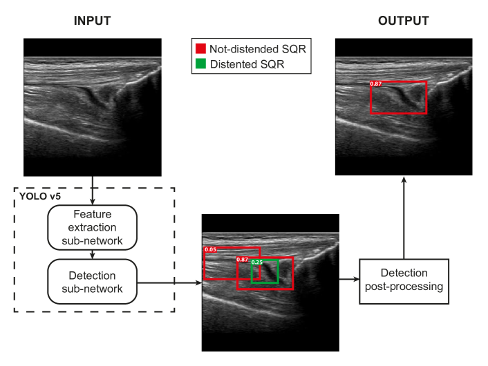
Figure 3: Overall architecture of the Detection approach

Each input US image is processed by the YoloV5 [46] object detector that returns a set of candidate SQRs, each characterized by a confidence value, a bounding box and the label (Distended or Non-distended). Since in the considered domain the input image actually contains exactly one SQR, the Detection Post-processing module selects the prediction with highest confidence and outputs its bounding box and its label.

We train the network to recognize two classes of objects: Distended SQRs and Non-distended SQRs. Since the amount of labeled images in in this domain is generally scarce, it is difficult to collect a sufficiently large dataset to fully train a robust detection network. Therefore, we adopt a transfer learning approach [47] to initialize the network’s weights. Specifically, we use the pre-trained weights publicly available for the YoloV5 network trained on the MS COCO dataset [48]. Finally, the network is fine-tuned on the actual dataset containing the labeled US images.

YoloV5 is a single stage detector designed to detect different objects in a image and directly assign them the corresponding class. YoloV5 is an optimized version of the YoloV4 framework [49], that has been widely used in the literature for object detection tasks. Specifically, among the five models available in YoloV5, we use the large model, which was empirically selected. YoloV5 is internally divided into a feature extraction sub-network and a detection sub-network. It also adopts a specific loss function and an early stop criterion. These four concepts are briefly described in the following.

Feature Extraction sub-network

The Feature Extraction sub-network is a Convolutional Neural Network (CNN). Specifically, it is a CSPDarknet53 network, that was originally proposed in [50] and that was shown to be particularly effective for object detection [49] and ultrasound image classification [51].

Detection sub-network

The Detection sub-network is divided into a neck and a head parts. The overall goal of the neck part is to divide the image into multiple small fragments with the objective of simplifying further analysis by performing semantic segmentation (by associating categories to pixels) as well as instance segmentation (classifiying and locating objects at pixel level). The head part is a one-stage detector [52] that processes the features returned by the neck part and outputs the bounding boxes of the detected elements along with their predicted class.

Loss function

We use the default YOLOV5 loss function that is shown in Equation 1 and that is computed as the weighted sum of three values: a) the localization loss ($L_{box}$) is computed with the Complete IoU loss function (CIoU) [53], and represents the error in the position of the predicted bounding box; b) the class loss ($L_{c}$) is computed with Binary Cross-Entropy (BCE) and represents the error in classifying the predicted class; c) the objectness loss ($L_{obj}$) is computed with BCE and represents to which extent the predicted bounding box actually encloses an object of interest. The weights of these values are hyper-parameters that need to be empirically tuned (see Section 6.3).

$$L=\alpha L_{box}+\beta L_{obj}+\gamma L_{c}$$ (1)

Early stopping criterion

We use the default YOLOV5 early stopping criterion to terminate the training if there are no improvements in the results for a given number of training epochs. This default criterion considers the mean Average Precision (mAP) of the detection, i.e., the ratio of correctly classified bounding boxes considering a given threshold of the IoU with the corresponding ground truth. Note that, in a multi-class scenario, this criterion factors for both the correct classification and the correct detection of the objects. Specifically it is computed as the weighted sum of the mAP@0.5 and the mAP@0.5:0.95 where a weight of $0.1$ is given for mAP@0.5, and a weight of $0.9$ is given for mAP@0.5:0.95 in order to prioritize more accurate bounding boxes detection.

4.2 Multi-task approach

The Detection approach addresses the problem of classifying the SQR as distended or not by selecting the label of the detection with the highest confidence. An alternative (and possibly more natural) solution would be to classify the entire image. However, this would not provide the needed SQR bounding box. For this reason we propose the Multi-task Approach that pairs image classification and detection.

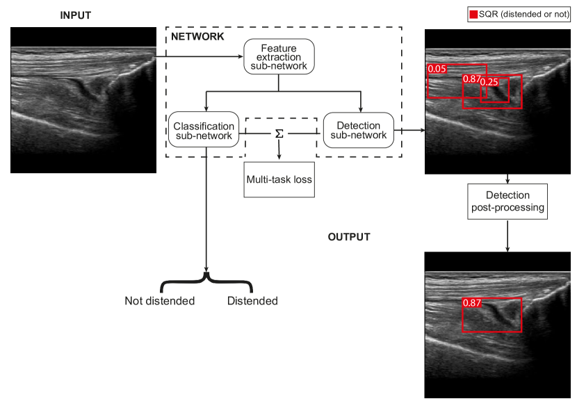
Figure 4: Overall architecture of the Multi-task approach

The proposed network is a modified version of the network used for the Detection approach. The key modification consists of a Classification sub-network that performs the SQR binary classification. The input image is first processed by the Feature Extraction sub-network, that is shared for both classification and detection tasks. Then the extracted features are simultaneously processed by the Detection sub-network and the Classification sub-network. The Classification sub-network processes the features and returns the predicted SQR class (i.e., distended or not) considering the whole image.

Differently from the Detection Approach solution, the goal of the Detection sub-network in the Multi-task solution is simply to detect the SQR, without providing information about the distension. Hence, the Detection sub-network network is trained with a single class and it returns a set of bounding boxes, all belonging to the same class, each with an associated confidence value. The Detection Post-processing module selects the bounding box with the highest confidence. During the training phase, the multi-task loss jointly considers the errors on classification and detection to update the network weights.

4.2.1 Classification sub-network

Figure 5 shows the Classification sub-network of the Multi-task Approach.

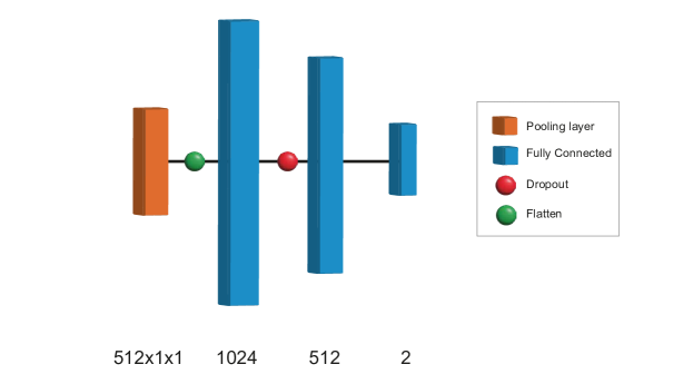
Figure 5: Classification sub-network architecture

The first layer of the sub-network is an Adaptive Average Pooling Layer in charge of reducing the feature dimensions to a fixed 2-dimensional output size. Then, the output is provided to a Flatten Layer, that converts 2-dimensional data to a 1-dimensional array. This array is then processed by a fully connected network composed of two hidden layers of $1024$ and $512$ units, respectively. These layers use a ReLu activation function. A dropout layer is applied between the two hidden layers with the objective of reducing overfitting. Finally, a Softmax layer is in charge of providing the most likely class (i.e., Distended/Non-distended). The architecture of this network has been determined empirically.

4.2.2 Multi-task loss

Training the multi-task network requires a custom loss function that simultaneously takes into account the classification and detection errors. For this reason, we adapt the loss function used for the Detection approach by adding a new loss term that represents the errors of the Classification sub-network. Specifically, we adopt a typical solution in binary classification that consists in computing the classification error $L_{cls}$ with a BCE function. Another difference with respect to the loss function used in the Detection approach, is that, in the Multi-Task Approach, the Detection sub-network is trained with a single class, hence there are no possible errors with class prediction. Thus, the $L_{c}$ parameter, considered in Equation 1, is always zero. So, the overall multi-task loss is computed as the weighted sum of $L_{box}$, $L_{obj}$, and $L_{cls}$, as shown in Equation 2. These weights are hyper-parameters that need to be empirically tuned (see Section 6.3).

$$L=\alpha L_{box}+\beta L_{obj}+\delta L_{cls}$$ (2)

Since the datasets in this domain are usually highly unbalanced (e.g., in our dataset $\approx 75\%$ of the images are labeled as Non-distended), there is the risk that the network favors Non-distended classifications, which in turn may increase the number of false negatives. In order to mitigate this problem, we adjust the classification loss $L_{cls}$ to give higher error values to false negatives (i.e., Distended SQR classified as Non-distended). This is achieved by adding an additional weight to $L_{cls}$ when the ground truth is Distended. In this case the weight is the ratio between the Non-distended and Distended samples in the training set. Thanks to this approach, the errors on the Distended samples have a more significant impact on the overall loss.

4.2.3 Multi-task early stopping criterion

As specified above, for the Detection approach, the default YOLOV5 early stopping criterion, based on mAP, is used to stop the training if no improvements are detected for a specified number of epochs. Instead, for the Multi-task approach, since the detection is computed for a single class, the mAP does not account for the classification accuracy but only considers the detection accuracy. Thus, for the Multi-task approach, we consider a weighted sum of mAP@0.5 for the detection and Balanced Accuracy (BA) for the classification on the validation set. In particular, we provide a higher weight ($0.7$) to the Balanced Accuracy and a lower one to to mAP@0.5 ($0.3$). This is due to the fact that we prefer to be more accurate on the classification, at the cost of identifying slightly less accurate (but still informative) bounding boxes. We consider a patience value of $100$ epochs, which means that the training is stopped if the early stopping criterion does not improve for the number of epoch specified by the patience value.

5 Dataset

Due to the lack of publicly available datasets in this field, we collected a dataset of SQR longitudinal scan images of $200$ adult patients with hemophilia, aged $44.7\pm 18.6$, between January 2021 and May 2022, thanks to the collaboration with ’Centro Emofilia e Trombosi Angelo Bianchi Bonomi’ of the polyclinic of Milan, a medical institution specialized in hemophilia. The study was approved by the institution’s ethics committee.

Before acquiring the dataset we first defined a standardized data acquisition protocol that includes: a) examination procedure based on the HEAD-US [7] protocol; b) guidelines on how to use the ultrasound device during the visit, for example defining that the joint side (left or right) should be annotated while acquiring the image itself; c) a procedure for data extraction from the ultrasound device; d) a data pseudo-anonymization procedure.

For each patient, the physician collected several US images from various scans in different joints. For this study we selected images of the SQR longitudinal scan. Two images of the SQR longitudinal scan are typically collected during each visit, one for each knee (left/right) but for some patients we only have one image while other patients were visited twice (often at a distance of several months), hence having up to four images each.

5.1 Data Acquisition

Images were acquired using the Philips Affiniti 50 US device by a single specialized practitioner during routine visits of hemophilic patients. When collecting the images, the probe was positioned as shown in Figure 1b and the knee was flexed by $30^{\circ}$. Each image has a resolution of $1024\times 780$ and, as shown in Figure 1a, it contains acquisition parameters (saved as text in the image) and the actual US scan (i.e., the yellow rectangle in Figure 1a). Note that the position and the dimension of the actual US scan (i.e., the yellow box) can vary. During the annotation process, the practitioner reported for each image whether the SQR was distended or not. Additionally, a trained operator, supervised by the practitioner, annotated the Minimum Bounding Rectangle (MBR) of the SQR.

A total of 483 knee subquadricipital recess longitudinal scans were annotated, 360 of which are labeled as Non-distended and 123 as Distended.

5.2 Pre-processing

We pre-process the collected images to extract the actual US image (e.g., the yellow box in Figure 1a). Indeed, as previously observed [45, 10] using the entire image as returned by the US device can reduce classification accuracy as this part of the image does not contain information needed for the required tasks.

As suggested by Tingelhoff et al [54] we initially cropped the images manually. However, this process is time consuming. We therefore developed an algorithm to automatically extract the US scan from the collected image. Figure 6 shows the steps of the pre-processing algorithm. In the first step, we measure and binarize the gradient of the image; we then remove connected pixel groups composed of less than $1000$ non-zero pixels; afterwards, we dilate the image to fill small groups of black pixels, and we perform an opening operation to remove groups of pixels not belonging to the US scan that were merged with it in the previous steps. Finally we crop the original image with the bounding box of the white area resulting from the previous step. Finally the images are resized to $256\times 256$ pixels.

All images have been double-checked as part of the annotation process and no cropping error was found, showing that the proposed automatic pre-processing is reliable.

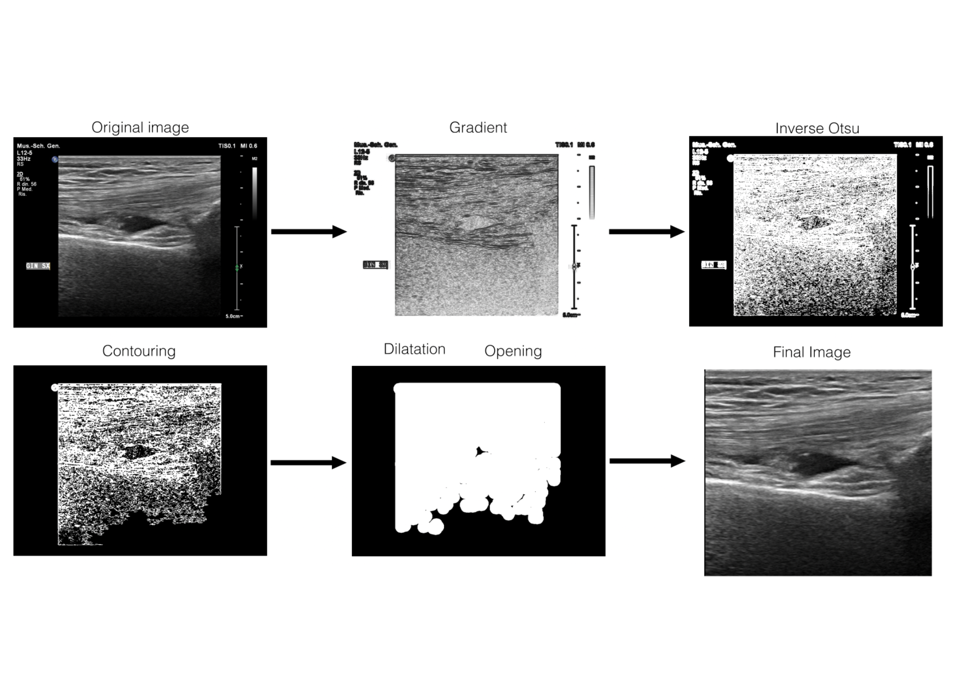
Figure 6: Intermediate steps of frame extraction procedure

6 Evaluation

In this section, we describe our experimental evaluation on the dataset that we introduced above. First, we present the adopted evaluation methodology and the metrics. Then, we describe how we selected the hyper-parameters. Finally, we show and compare the results of the two proposed solutions and present some examples.

6.1 Metrics

We define two sets of metrics: one for the detection and the other for the classification. For what concerns the detection, we measure the average Intersection over Union (IoU). The IoU between two plane figures is defined as the ratio between the area of their intersection and the area of their union. For each test image we measure the IoU between the bounding box predicted with the highest confidence and the ground truth bounding box. Then, we compute the average of this metric among all images.

Considering classification, for each image we compare the ground truth class with the predicted class hence computing if the result is a True Positive (TP), a True Negative (TN), a False Positive (FP), or a False Negative (FN). Note that the positive class is Distended and the negative class is Non-distended. Then, we used the following classification metrics:

• Specificity: measures the ability of the model to identify true negatives. Specificity$={TN\over{TN+FP}}$

• Sensitivity: measures the ability of the model to identify true positives. Sensitivity$={TP\over{TP+FN}}$

• Balanced Accuracy: mean between specificity and sensitivity. It is considered a sounder metric compared to accuracy when the class imbalance is high [55]. Balanced accuracy $={{sens+spec}\over 2}$

6.2 Evaluation methodology

The evaluation of the recognition rate of the proposed solutions is based on a 5-fold cross-validation. In order to avoid high correlation bias, the training and the test splits do not have images from the same patients in common. The consequence is that we could not exactly divide the dataset in $80\%$ and $20\%$ splits and therefore the splits have slightly different number of images. An example fold subdivision can be found in Table 1. Each training fold was further split: $80\%$ as training set and $20\%$ as validation set. During training we used SGD with momentum [56] as optimizer.

Fold 0	Train	Test	Total
Non-distended	289	71	360
Distended	97	26	123
Total	386	97	483
Total patients	166	42	208

Table 1: Example data distribution in Fold 0 of 5-f CV

6.3 Hyper-parameters selection

In order to properly tune the many hyper-parameters of our network, we adopt an evolutionary approach [57]. Given a fitness function, an evolutionary algorithm evaluates the best fitting set of hyper-parameters thanks to mutation and cross-over operations. For the sake of this work, we considered the evolutionary method proposed in YOLOV5, that only considers the mutation operation with $90\%$ of probability and $0.04$ of variance. Each mutation step generates a new set of hyper-parameters given a combination of the best parents from all the previous generations. The fitness functions used for the hyper-parameters selection for the Detection approach and the Multi-task approach correspond to the early stopping criteria introduced in Sections 4.1 and 4.2.3, respectively.

In order to balance the need for a high number of evolution epochs with limited computational resources, we run the evolutionary algorithm only on one fold.

We executed our evolutionary algorithm for $300$ epochs on each solution. Considering the Multi-task Approach, the best results have been obtained at the $193$th epoch, while for the Detection approach the best set of hyper-parameters were found at the $4$th epoch. The set of hyper-parameters resulting from evolution have been used to evaluate our approaches on the complete cross validation procedure. The most relevant discovered hyper-parameters are presented in Table 2

	Learning rate	Dropout	SGD momentum	$\alpha$	$\beta$	$\gamma$	$\delta$
Detection	0.00369	-	0.77628	0.06868	0.49062	0.2343	-
Multi-task	0.0018	0.11008	0.62403	0.05427	0.67598	-	0.41855

Table 2: Selected hyper-parameters

Note that $\gamma$ is a weight associated to the $L_{c}$ loss that is only considered in the Detection approach, while $\delta$ is a weight associated to the $L_{cls}$ loss that is only considered in Multi-task approach. Finally, the Dropout rate is only included in the Classification sub-network of the Multi-task approach.

6.4 Results

Table 3 shows the performance of the two proposed solutions.

	Balanced accuracy	Specificity	Sensitivity	IoU
Detection Approach	0.74 $\pm$ 0.07	0.97 $\pm$0.03	0.52 $\pm$ 0.12	0.66 $\pm$ 0.01
Multi-task Approach	0.78 $\pm$ 0.05	0.92 $\pm$ 0.04	0.64 $\pm$ 0.09	0.63 $\pm$ 0.02

Table 3: Evaluation results (reported as mean among the folds $\pm$ standard deviation)

Since both the early stopping criterion and the hyper-parameters selection methods for the Multi-task approach are designed to prioritize the classification accuracy at the expense of the detection accuracy, its balanced accuracy is confirmed to be more accurate with respect to the Detection approach. This increase is particularly relevant as it brings the balanced accuracy over the threshold of $0.75$ that is reported to be a requirement for a medical test to be “useful” [58].

The increase in the balanced accuracy comes at the expense of a reduction in the detection accuracy. Indeed, the IoU metric decreases from $0.66$ for the Detection Approach to $0.63$ for the Multi-task Approach. However, if we consider the percentage of the images for which the IoU between the detection and the ground truth is $\geq 0.5$, which is a common threshold used for similar tasks, we notice that the decrease is relatively small. Indeed, the result for the Detection Approach is $85\%$ and it decreases to $82\%$ for the Multi-task Approach.

The increase in balanced accuracy value of the Multi-task Approach is largely influenced by the increase in sensitivity. The reason for this increase is likely due to the adjusted classification loss in the Multi-task Approach introduced to mitigate the unbalanced data problem (see Section 4.2.2). Indeed, considering the confusion matrices in Figure 7 we can observe that the Detection Approach has $59$ false negatives ($48\%$), out of a total of $123$ images labelled as Distended, compared to the $44$ false negatives in the Multi-task Approach ($38\%$). This improvement comes at a cost of a lower specificity value. Indeed, the Detection Approach has $11$ false positives out of $360$ negative images ($3\%$) while the Multi-task Approach has $29$ false positives ($8\%$).

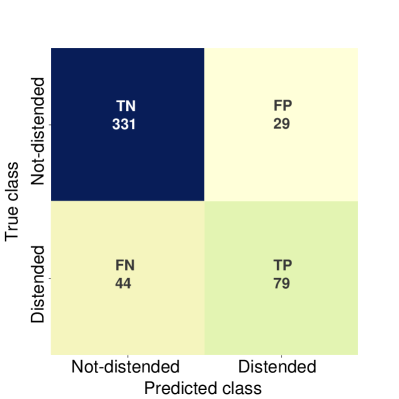
(a) Multi-task learning

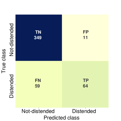
(b) Detection

Figure 7: Confusion matrices

6.5 Examples

In order to better illustrate how our approaches work, in the following we show some examples of correct and incorrect output.

Figure 8 shows two US images that have been correctly classified by both approaches and that are relatively easy to classify by medical experts. Figure 8a shows an US image where the femur, the patella and the SQR are clearly visible, and the SQR is thin (i.e., not distended). On the other hand, Figure 8b shows an example of a Distended SQR. In this case, the SQR is clearly thick and hence distended.

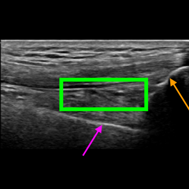
(a) Non-Distended SQR

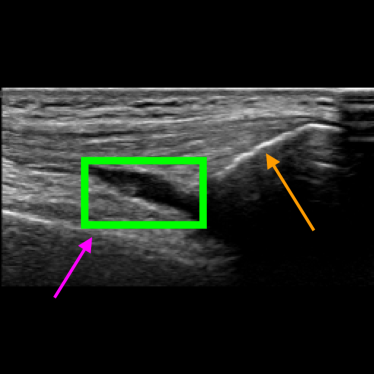
(b) Distended SQR

Figure 8: Examples of images correctly classified by both solutions. The purple arrow points to the femur, the orange arrow points to the patella, and the green box indicates the SQR.

Figure 9 shows four examples of images that are more challenging to classify even by medical experts. This usually happens when there is noise in the US scan (as in Figure 9c) or when the SQR is borderline between Distended and Non-distended (as in Figure 9d). Figure 9a is correctly classified by both approaches as Non-distended. Figure 9b is correctly classified by the Multi-task approach but not by the Detection approach. Vice versa, Figure 9c is correctly classified by the Detection approach and not by the Multi-task approach. Finally, both solutions wrongly classify Figure 9d.

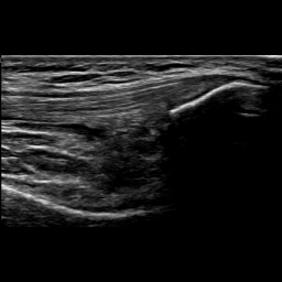
(a) Non-distended SQR

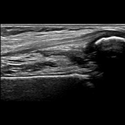
(b) Distended SQR

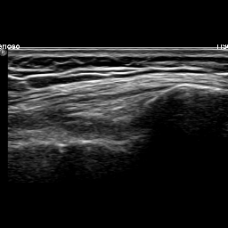
(c) Non-distended SQR

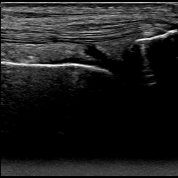
(d) Distended SQR

Figure 9: Examples of images that are intuitively hard to classify.

Considering the detection problem, Figure 10 shows US images where the two approaches detected the SQR with the lowest and the highest IoU. In Figure 10a, the Multi-task approach wrongly detects as SQR an image region that is similar to an actual SQR in terms of position and shape, resulting in a very low value of IoU ($0.33$). In this case, also the Detection approach can not reliably detect the right target precisely, and indeed it detects only a small portion of the actual SQR (IoU=$0.33$). Instead, in the example shown in Figure 10b the Multi-task approach accurately detects the SQR (IoU=$0.95$), while the Detection approach identifies the same area with a lower IoU ($0.68)$.

Figure 10c shows the US image for which the Detection approach provided the lowest IoU value. The problem is similar to that of Figure 10a: a region is erroneously recognized as a SQR because it is similar to a SQR. In this case the detected bounding box does not overlap with the ground truth, hence the IoU is zero. Instead, the Multi-Task approach basically detects the right target (IOU=$0.58$).

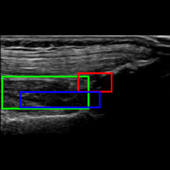
(a) Worst detection by Multi-Task approach

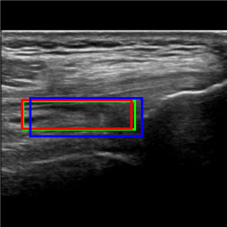
(b) Best detection by Multi-Task approach

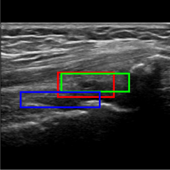
(c) Worst detection by Detection approach

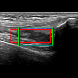
(d) Best detection by Detection approach

Figure 10: Detection examples. Green represents the ground truth, red and blue the results of the Multi-Task approach and Detection approach, respectively.

Figure 10d shows instead the US image for which the Detection approach provided the highest IoU value ($0.96$). In this case the Multi-task approach identifies the right target less precisely, resulting in a IoU of $0.55$.

7 Conclusion

Early detection of hemarthrosis is fundamental to reduce the risk of under and over treatment for hemophilic patients. A Computer-Aided Diagnosis (CAD) tool that detects joint recess distension from ultrasound (US) images can support practitioners in diagnosing hemarthrosis without the need for expensive and time consuming exams (like MRI). We investigate the requirements of such a tool and we frame the problem in terms of a combination of two typical machine learning tasks: classification and detection. Addressing this problem is particularly challenging for a number of reasons, including that the position and the shape of the joint recess may change considerably across different US images, and there can even be borderline cases in which the recess is only partially distended. Finally, the datasets in this problem domain are generally small and may contain noisy images.

This paper presents two solutions, each providing both recess detection and classification. Experiments, conducted on images of the Subquadricipital Recess (SQR), i.e., the knee joint recess, focusing on a specific US scan (the SQR longitudinal scan) show promising results. Indeed, both solutions achieve a Balanced Accuracy (BA) of approximately $0.75$, a threshold value used in the literature to distinguish “useful” medical tests [58]. In particular the MultiTask approach achieves a BA value of $0.78$. For what concerns the detection, the two solutions guarantee a correct detection (i.e., IoU $>0.5$) in more then $82\%$ of the cases.

We believe that the performance of our solutions can be considerably improved in two possible ways. First, the CAD tool could process multiple images of the same joint, possible from different scans or from a video feed. The different results computed on the various images can then be combined to provide a more reliable outcome. The second improvement could be the adoption of an ensemble approach, in which a number of different models are trained and the CAD tool computes the result as a combination of the individual results provided by each model. Beyond improving the performance, these possible improvements have a potential important advantage: they can identify borderline cases (e.g., when there is a disagreement in classification by two or more models, or by processing two scans of the same knee). In these (hopefully rare) cases, the CAD tool can inform the practitioner who can decide, for example, to use a different diagnosing tool (e.g., MRI).

As a future work we intend to apply the proposed solutions on multiple scans for multiple joints. Actually, we are currently collecting images and videos on a total of $6$ scans for the knee, the elbow, and the ankle. Our final goal is to create a bed-side solution for early hemarthrosis diagnosis. The idea is to enable an operator with little training (e.g., the patient or a caregiver) to acquire US images with a portable US device. The system will support the operator during the acquisition by identifying the relevant reference points (e.g., the patella), by guiding the operator to correctly position the US probe, and by evaluating the images in real time to inform the operator that a suitable image was collected. The US images will then be transmitted to the practitioner or even automatically processed as a part of a screening procedure.

References

- [1] Goris Roosendaal and Floris P. J. G Lafeber. Blood-induced joint damage in hemophilia: Modern management of hemophilia a to prevent bleeding and arthropathy. Seminars in thrombosis and hemostasis, 29(1):37–42, 2003.
- [2] Alok Srivastava, Elena Santagostino, Alison Dougall, Steve Kitchen, Megan Sutherland, Steven W Pipe, Manuel Carcao, Johnny Mahlangu, Margaret V Ragni, Jerzy Windyga, et al. Wfh guidelines for the management of hemophilia. Haemophilia, 26:1–158, 2020.
- [3] Margaret W Hilgartner. Current treatment of hemophilic arthropathy. Current opinion in pediatrics, 14(1):46–49, 2002.
- [4] Domen Plut, Barbara Faganel Kotnik, Irena Preloznik Zupan, Damjana Kljucevsek, Gaj Vidmar, Ziga Snoj, Carlo Martinoli, and Vladka Salapura. Diagnostic accuracy of haemophilia early arthropathy detection with ultrasound (head-us): a comparative magnetic resonance imaging (mri) study. Radiology and oncology, 53(2):178–186, 2019.
- [5] P N T Wells. Ultrasound imaging. Physics in medicine & biology, 51(13):R83–R98, 2006.
- [6] Fredrick Joshua, Marissa Lassere, Alexander K Scheel, David Kane, Walter Grassi, Philip G Conaghan, Richard J Wakefield, Maria-Antonietta D’Agostino, George A Bruyn, Marcin Szkudlarek, Esperanza Naredo, Wolfgang A Schmidt, Peter Balint, Emilio Filippucci, Marina Backhaus, and Annamaria Iagnocco. Summary findings of a systematic review of the ultrasound assessment of synovitis. Journal of rheumatology, 34(4):839–847, 2007.
- [7] Carlo Martinoli, Ornella Della Casa Alberighi, Giovanni Di Minno, Ermelinda Graziano, Angelo Claudio Molinari, Gianluigi Pasta, Giuseppe Russo, Elena Santagostino, Annarita Tagliaferri, Alberto Tagliafico, and Massimo Morfini. Development and definition of a simplified scanning procedure and scoring method for haemophilia early arthropathy detection with ultrasound (head-us). Thrombosis and haemostasis, 109(6):1170–1179, 2013.
- [8] Heang-Ping Chan, E Charles, P Metz, KL Lam, Y Wu, and H Macmahon. Improvement in radiologists’ detection of clustered microcalcifications on mammograms. Arbor, 1001:48109–0326, 1990.
- [9] Kunio Doi. Current status and future potential of computer-aided diagnosis in medical imaging. The British journal of radiology, 78(suppl_1):s3–s19, 2005.
- [10] Zhili Long, Xiaobing Zhang, Cong Li, Jin Niu, Xiaojun Wu, and Zuohua Li. Segmentation and classification of knee joint ultrasonic image via deep learning. Applied Soft Computing, 97:106765, 2020.
- [11] P Tyrrell, V Blanchette, M Mendez, D Paniukov, B Brand, M Zak, and J Roth. Detection of joint effusions in pediatric patients with hemophilia using artificial intelligence-assisted ultrasound scanning; early insights from the development of a self-management tool. Res Pract Thromb Haemost, 5, 2021.
- [12] Vincent Chan and Anahi Perlas. Basics of ultrasound imaging. In Atlas of ultrasound-guided procedures in interventional pain management, pages 13–19. Springer, 2011.
- [13] Laura J Brattain, Brian A Telfer, Manish Dhyani, Joseph R Grajo, and Anthony E Samir. Machine learning for medical ultrasound: status, methods, and future opportunities. Abdominal radiology, 43(4):786–799, 2018.
- [14] Roberta Gualtierotti, Luigi Piero Solimeno, and Flora Peyvandi. Hemophilic arthropathy: current knowledge and future perspectives. Journal of Thrombosis and Haemostasis, 19(9):2112–2121, 2021.
- [15] Hiroshi Fujita. Ai-based computer-aided diagnosis (ai-cad): the latest review to read first. Radiological physics and technology, 13(1):6–19, 2020.
- [16] Qinghua Huang, Fan Zhang, and Xuelong Li. Machine learning in ultrasound computer-aided diagnostic systems: a survey. BioMed research international, 2018, 2018.
- [17] Min Chen, Xiaobo Shi, Yin Zhang, Di Wu, and Mohsen Guizani. Deep feature learning for medical image analysis with convolutional autoencoder neural network. IEEE transactions on big data, 7(4):750–758, 2021.
- [18] Karen Simonyan and Andrew Zisserman. Very deep convolutional networks for large-scale image recognition. arXiv preprint arXiv:1409.1556, 2014.
- [19] Zeynettin Akkus, Jason Cai, Arunnit Boonrod, Atefeh Zeinoddini, Alexander D Weston, Kenneth A Philbrick, and Bradley J Erickson. A survey of deep-learning applications in ultrasound: Artificial intelligence-powered ultrasound for improving clinical workflow. Journal of the American College of Radiology, 16(9):1318–1328, 2019.
- [20] Neha Sharma, Vibhor Jain, and Anju Mishra. An analysis of convolutional neural networks for image classification. Procedia computer science, 132:377–384, 2018.
- [21] Phillip M Cheng and Harshawn S Malhi. Transfer learning with convolutional neural networks for classification of abdominal ultrasound images. Journal of digital imaging, 30(2):234–243, 2017.
- [22] Tianjiao Liu, Shuaining Xie, Jing Yu, Lijuan Niu, and Weidong Sun. Classification of thyroid nodules in ultrasound images using deep model based transfer learning and hybrid features. In 2017 IEEE International Conference on Acoustics, Speech and Signal Processing (ICASSP), pages 919–923. IEEE, 2017.
- [23] Walid Al-Dhabyani, Mohammed Gomaa, Hussien Khaled, and Aly Fahmy. Deep learning approaches for data augmentation and classification of breast masses using ultrasound images. International journal of advanced computer science & applications, 10(5), 2019.
- [24] Tomoyuki Fujioka, Mio Mori, Kazunori Kubota, Yuka Kikuchi, Leona Katsuta, Mio Adachi, Goshi Oda, Tsuyoshi Nakagawa, Yoshio Kitazume, and Ukihide Tateishi. Breast ultrasound image synthesis using deep convolutional generative adversarial networks. Diagnostics (Basel), 9(4):176–, 2019.
- [25] Seokmin Han, Ho-Kyung Kang, Ja-Yeon Jeong, Moon-Ho Park, Wonsik Kim, Won-Chul Bang, and Yeong-Kyeong Seong. A deep learning framework for supporting the classification of breast lesions in ultrasound images. Physics in Medicine & Biology, 62(19):7714, 2017.
- [26] Dan Meng, Libo Zhang, Guitao Cao, Wenming Cao, Guixu Zhang, and Bing Hu. Liver fibrosis classification based on transfer learning and fcnet for ultrasound images. IEEE access, 5:5804–5810, 2017.
- [27] Hiroki Tanaka, Shih-Wei Chiu, Takanori Watanabe, Setsuko Kaoku, and Takuhiro Yamaguchi. Computer-aided diagnosis system for breast ultrasound images using deep learning. Physics in Medicine & Biology, 64(23):235013, 2019.
- [28] Anton S Becker, Michael Mueller, Elina Stoffel, Magda Marcon, Soleen Ghafoor, and Andreas Boss. Classification of breast cancer in ultrasound imaging using a generic deep learning analysis software: a pilot study. The British journal of radiology, 91(xxxx):20170576, 2018.
- [29] Yi Wang, Eun Jung Choi, Younhee Choi, Hao Zhang, Gong Yong Jin, and Seok-Bum Ko. Breast cancer classification in automated breast ultrasound using multiview convolutional neural network with transfer learning. Ultrasound in medicine & biology, 46(5):1119–1132, 2020.
- [30] U Rajendra Acharya, Oliver Faust, Filippo Molinari, S Vinitha Sree, Sameer P Junnarkar, and Vidya Sudarshan. Ultrasound-based tissue characterization and classification of fatty liver disease: A screening and diagnostic paradigm. Knowledge-Based Systems, 75:66–77, 2015.
- [31] Dan Meng, Libo Zhang, Guitao Cao, Wenming Cao, Guixu Zhang, and Bing Hu. Liver fibrosis classification based on transfer learning and fcnet for ultrasound images. Ieee Access, 5:5804–5810, 2017.
- [32] Tianjiao Liu, Shuaining Xie, Jing Yu, Lijuan Niu, and Weidong Sun. Classification of thyroid nodules in ultrasound images using deep model based transfer learning and hybrid features. In 2017 IEEE International Conference on Acoustics, Speech and Signal Processing (ICASSP), pages 919–923. IEEE, 2017.
- [33] Junho Song, Young Jun Chai, Hiroo Masuoka, Sun-Won Park, Su-jin Kim, June Young Choi, Hyoun-Joong Kong, Kyu Eun Lee, Joongseek Lee, Nojun Kwak, et al. Ultrasound image analysis using deep learning algorithm for the diagnosis of thyroid nodules. Medicine, 98(15), 2019.
- [34] Gayatri Kompella, Maria Antico, Fumio Sasazawa, S. Jeevakala, Keerthi Ram, Davide Fontanarosa, Ajay K Pandey, and Mohanasankar Sivaprakasam. Segmentation of femoral cartilage from knee ultrasound images using mask r-cnn. In 2019 41st Annual International Conference of the IEEE Engineering in Medicine and Biology Society (EMBC), pages 966–969, 2019.
- [35] Zhantao Cao, Lixin Duan, Guowu Yang, Ting Yue, and Qin Chen. An experimental study on breast lesion detection and classification from ultrasound images using deep learning architectures. BMC medical imaging, 19(1):1–9, 2019.
- [36] Xianhua Zeng, Li Wen, Banggui Liu, and Xiaojun Qi. Deep learning for ultrasound image caption generation based on object detection. Neurocomputing, 392:132–141, 2020.
- [37] Christian F Baumgartner, Konstantinos Kamnitsas, Jacqueline Matthew, Tara P Fletcher, Sandra Smith, Lisa M Koch, Bernhard Kainz, and Daniel Rueckert. Sononet: real-time detection and localisation of fetal standard scan planes in freehand ultrasound. IEEE transactions on medical imaging, 36(11):2204–2215, 2017.
- [38] Ke Yan, Youbao Tang, Yifan Peng, Veit Sandfort, Mohammadhadi Bagheri, Zhiyong Lu, and Ronald M Summers. Mulan: multitask universal lesion analysis network for joint lesion detection, tagging, and segmentation. In International Conference on Medical Image Computing and Computer-Assisted Intervention, pages 194–202. Springer, 2019.
- [39] Fei Gao, Hyunsoo Yoon, Teresa Wu, and Xianghua Chu. A feature transfer enabled multi-task deep learning model on medical imaging. Expert Systems with Applications, 143:112957, 2020.
- [40] Maria V Sainz de Cea, Karl Diedrich, Ran Bakalo, Lior Ness, and David Richmond. Multi-task learning for detection and classification of cancer in screening mammography. In International Conference on Medical Image Computing and Computer-Assisted Intervention, pages 241–250. Springer, 2020.
- [41] Tsung-Yi Lin, Priya Goyal, Ross Girshick, Kaiming He, and Piotr Dollár. Focal loss for dense object detection. In Proceedings of the IEEE international conference on computer vision, pages 2980–2988, 2017.
- [42] Thi-Lam-Thuy Le, Nicolas Thome, Sylvain Bernard, Vincent Bismuth, and Fanny Patoureaux. Multitask classification and segmentation for cancer diagnosis in mammography. arXiv preprint arXiv:1909.05397, 2019.
- [43] Haifan Gong, Guanqi Chen, Ranran Wang, Xiang Xie, Mingzhi Mao, Yizhou Yu, Fei Chen, and Guanbin Li. Multi-task learning for thyroid nodule segmentation with thyroid region prior. In 2021 IEEE 18th International Symposium on Biomedical Imaging (ISBI), pages 257–261. IEEE, 2021.
- [44] Guisheng Zhang, Kehui Zhao, Yanfei Hong, Xiaoyu Qiu, Kuixing Zhang, and Benzheng Wei. Sha-mtl: soft and hard attention multi-task learning for automated breast cancer ultrasound image segmentation and classification. International Journal of Computer Assisted Radiology and Surgery, 16(10):1719–1725, 2021.
- [45] Bor-Shing Lin, Jean-Lon Chen, Yi-Hsuan Tu, Ya-Xing Shih, Yu-Ching Lin, Wen-Ling Chi, and Yi-Cheng Wu. Using deep learning in ultrasound imaging of bicipital peritendinous effusion to grade inflammation severity. IEEE journal of biomedical and health informatics, 24(4):1037–1045, 2020.
- [46] Glenn Jocher, Ayush Chaurasia, Alex Stoken, Jirka Borovec, NanoCode012, Yonghye Kwon, TaoXie, Jiacong Fang, imyhxy, Kalen Michael, Lorna, Abhiram V, Diego Montes, Jebastin Nadar, Laughing, tkianai, yxNONG, Piotr Skalski, Zhiqiang Wang, Adam Hogan, Cristi Fati, Lorenzo Mammana, AlexWang1900, Deep Patel, Ding Yiwei, Felix You, Jan Hajek, Laurentiu Diaconu, and Mai Thanh Minh. ultralytics/yolov5: v6.1 - TensorRT, TensorFlow Edge TPU and OpenVINO Export and Inference, February 2022.
- [47] Phillip M Cheng and Harshawn S Malhi. Transfer learning with convolutional neural networks for classification of abdominal ultrasound images. Journal of digital imaging, 30(2):234–243, 2017.
- [48] Tsung-Yi Lin, Michael Maire, Serge Belongie, James Hays, Pietro Perona, Deva Ramanan, Piotr Dollár, and C Lawrence Zitnick. Microsoft coco: Common objects in context. In European conference on computer vision, pages 740–755. Springer, 2014.
- [49] Alexey Bochkovskiy, Chien-Yao Wang, and Hong-Yuan Mark Liao. Yolov4: Optimal speed and accuracy of object detection. arXiv preprint arXiv:2004.10934, 2020.
- [50] Chien-Yao Wang, Hong-Yuan Mark Liao, Yueh-Hua Wu, Ping-Yang Chen, Jun-Wei Hsieh, and I-Hau Yeh. Cspnet: A new backbone that can enhance learning capability of cnn. In 2020 IEEE/CVF Conference on Computer Vision and Pattern Recognition Workshops (CVPRW), pages 1571–1580, 2020.
- [51] Kiran Jabeen, Muhammad Attique Khan, Majed Alhaisoni, Usman Tariq, Yu-Dong Zhang, Ameer Hamza, Artūras Mickus, and Robertas Damaševičius. Breast cancer classification from ultrasound images using probability-based optimal deep learning feature fusion. Sensors, 22(3):807, 2022.
- [52] Joseph Redmon and Ali Farhadi. Yolov3: An incremental improvement. arXiv.org, 2018.
- [53] Zhaohui Zheng, Ping Wang, Wei Liu, Jinze Li, Rongguang Ye, and Dongwei Ren. Distance-iou loss: Faster and better learning for bounding box regression. In Proceedings of the AAAI conference on artificial intelligence, volume 34, pages 12993–13000, 2020.
- [54] Kathrin Tingelhoff, Klaus WG Eichhorn, Ingo Wagner, Maria E Kunkel, Analia I Moral, Markus E Rilk, Friedrich M Wahl, and Friedrich Bootz. Analysis of manual segmentation in paranasal ct images. European archives of oto-rhino-laryngology, 265(9):1061–1070, 2008.
- [55] Kay Henning Brodersen, Cheng Soon Ong, Klaas Enno Stephan, and Joachim M Buhmann. The balanced accuracy and its posterior distribution. In 2010 20th international conference on pattern recognition, pages 3121–3124. IEEE, 2010.
- [56] Ilya Sutskever, James Martens, George Dahl, and Geoffrey Hinton. On the importance of initialization and momentum in deep learning. In International conference on machine learning, pages 1139–1147. PMLR, 2013.
- [57] Erik Bochinski, Tobias Senst, and Thomas Sikora. Hyper-parameter optimization for convolutional neural network committees based on evolutionary algorithms. In 2017 IEEE international conference on image processing (ICIP), pages 3924–3928. IEEE, 2017.
- [58] Michael Power, Greg Fell, and Michael Wright. Principles for high-quality, high-value testing. BMJ Evidence-Based Medicine, 18(1):5–10, 2013.