Time Series Forecasting with Hypernetworks Generating Parameters in Advance

Abstract.

Forecasting future outcomes from recent time series data is not easy, especially when the future data are different from the past (i.e. time series are under temporal drifts). Existing approaches show limited performances under data drifts, and we identify the main reason: It takes time for a model to collect sufficient training data and adjust its parameters for complicated temporal patterns whenever the underlying dynamics change. To address this issue, we study a new approach; instead of adjusting model parameters (by continuously re-training a model on new data), we build a hypernetwork that generates other target models’ parameters expected to perform well on the future data. Therefore, we can adjust the model parameters beforehand (if the hypernetwork is correct). We conduct extensive experiments with 6 target models, 6 baselines, and 4 datasets, and show that our HyperGPA outperforms other baselines.

1. INTRODUCTION

Time series forecasting is one of the most fundamental problems in deep learning, ranging from classical climate modeling (Brouwer et al., 2019; REN, 2021) and stock price forecasting (Ariyo et al., 2014; Vijh et al., 2020) to recent pandemic forecasting (Wu et al., 2020; Wang et al., 2021b). Since these tasks are important in many real-world applications, diverse methods have been proposed, such as recurrent neural networks (RNNs) (Hochreiter and Schmidhuber, 1997; Cho et al., 2014), neural ordinary differential equations (NODEs) (Chen et al., 2019), neural controlled differential equations (NCDEs) (Kidger et al., 2020), and so on. Owing to these novel models, the forecasting accuracy has been significantly enhanced over the past several years.

However, this forecasting is challenging, especially when temporal drifts, i.e., a data distribution changes over time by an underlying latent dynamics, exist in time series data (cf. Fig. 1) (Zhang et al., 2013; Oh et al., 2019; Li et al., 2021; Kuznetsov and Mohri, 2014; Kuznetsov et al., 2015). For example, the number of COVID-19 patients fluctuates severely over time, and a dynamics behind the daily patient numbers is governed by complicated factors.

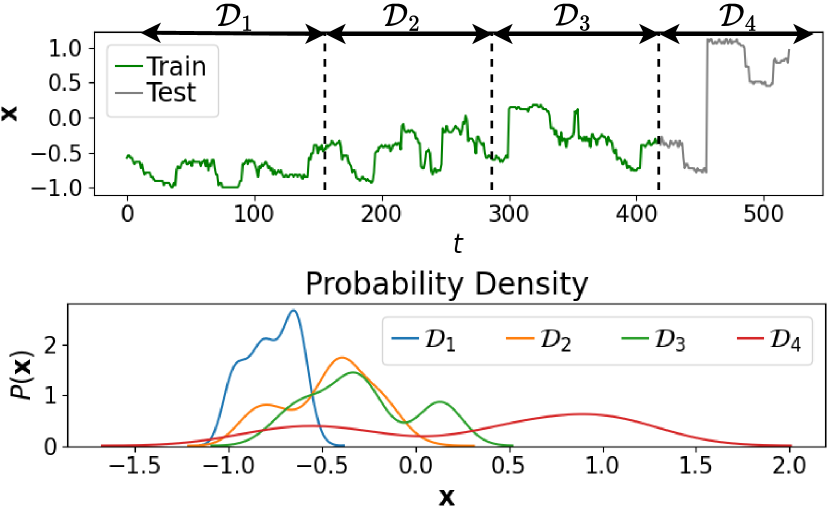
Figure 1. Time series data under temporal drifts. $\mathcal{D}_{4}$ is an unseen period to be forecast. Each period $\mathcal{D}_{j}$ shows a different probability density.

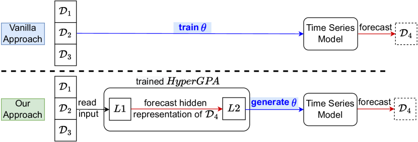
Figure 2. In a vanilla setting, a time series model is trained with all historical periods. On the contrary, in HyperGPA, the first layer ($L1$) understands the recent periods ($\mathcal{D}_{1},\mathcal{D}_{2},\mathcal{D}_{3}$) and forecasts a hidden representation for the next period ($\mathcal{D}_{4}$) with the discovered underlying dynamics. Based on the forecast hidden representation, the second layer ($L2$) generates the parameters of a time series model which would work well for $\mathcal{D}_{4}$.

To defend against the latent dynamics, we propose a new approach that enables highly accurate time series forecasting under temporal drifts. Specifically, we present a Hypernetwork Generating Parameters in Advance (HyperGPA). In usual settings, to forecast future data, one can train the parameters of a target time series model with data from all historical periods. On the other hand, HyperGPA is based on hypernetworks which are neural networks generating the parameters of other neural networks (called target models) (Ha et al., 2016). Our hypernetwork has two parts as depicted in Fig. 2: one ($L1$) captures the hidden dynamics given recent time series data, and the other ($L2$) generates (i.e., forecasts) a set of parameters for a target time series forecasting model. To our knowledge, we are the first proposing a hypernetwork-based approach for addressing temporal drift problems.

In HyperGPA, $L1$ is responsible for discovering a hidden underlying dynamics and forecasting a future period’s characteristic from data in recent periods. We use NCDEs for $L1$ since they are a continuous analogue to RNNs and are known to be superior to RNNs in processing a complicated dynamics (Jhin et al., 2022; Jeon et al., 2022). To reflect real-world scenarios, we assume $M$ loosely coupled time series data. For instance, the United States flu dataset (CDC, 1946) contains weekly reports for each state, which consists of 51 loosely coupled time series, i.e., one time series for each state. Because the underlying dynamics of the correlated multiple time series are also correlated, considering them at the same time can make the task easier by increasing the number of training samples. To process multiple time series simultaneously, we integrate recent graph convolutional networks (GCNs) and NCDEs into a single framework — we learn the latent graph of those $M$ loosely coupled time series from data and apply the GCN technology (Bai et al., 2020). Therefore, the first part of our hypernetwork can be understood as a shared multi-task layer in that it processes multiple time series simultaneously.

From the hidden representation of the future period forecast by $L1$, $L2$ generates the future parameters of a target time series model. The parameters are generated based on GCNs since target neural network models are typically represented by computation graphs. However, if we generate parameters for each time series and for each period independently, the target models equipped with the generated parameters are vulnerable to an overfitting problem. This is because we assume $M$ loosely coupled time series and different periods of a time series are also correlated to each other to some extent, although they may have different distributions. To solve this problem, we propose an attention-based generation method (Vaswani et al., 2017), where we first generate several candidate sets of parameters and then combine them via the attention coefficients to obtain the final parameters. Our proposed attention-based method has the following advantages: i) the number of parameters of HyperGPA itself is not large; ii) HyperGPA can relieve an overfitting problem of target models; iii) HyperGPA can be successfully applied to almost all existing popular time series forecasting models, ranging from RNNs and NODEs to NCDEs, which is a significant enhancement in comparison with other hypernetwork-based approaches which assume a specific target model type (Ha et al., 2016; Zhang et al., 2019). To summarize, we make the following contributions:

1. Novel Approach to Temporal Drifts: We propose a hypernetwork, called HyperGPA, that can forecast the future parameters of target time series models from previous periods. Aided by the NCDE technology, we show that our model is able to capture the pattern of temporal drift dynamics.

2. Novel Approach to Hypernetwork: HyperGPA generates parameters for each period via our proposed attention-based method, alleviating overfitting and resulting in a small model size. Also, it can be applied to almost all existing popular time series forecasting models, ranging from LSTMs/GRUs to NODEs/NCDEs.

3. Effectiveness: HyperGPA improves target models’ errors up to 64.1% with their small parameter sizes, compared to six baselines which include not only existing approaches addressing the temporal drift problem, but also hypernetwork-based approaches.

4. Reproducibility: Our code is available in the supplementary material and we refer the reader to Appendix C for the details of reproducing our experimental results.

2. RELATED WORK & MOTIVATION

2.1. Hypernetwork

In general, neural networks generating the parameters of other neural networks are called hypernetworks. We call a neural network whose parameters are generated by a hypernetwork as a target model. Hypernetworks can be used for many purposes. Interpreted as implicit distributions, hypernetworks give help for uncertainty estimations, which are new methods for more flexible variational approximation learning (Pawlowski et al., 2018; Henning et al., 2018; Krueger et al., 2017). (Oswald et al., 2020) used hypernetworks for continual learning. Hypernetworks were also used for neural architecture search (Zhang et al., 2018), and for personalized federated learning which aims to train models for multiple clients with respective data distributions (Shamsian et al., 2021).

Futhermore, hypernetworks helped target models to have high representation learning capabilities, by allowing the parameters of target models to be changed (Nachmani and Wolf, 2019; Littwin and Wolf, 2019; Pan et al., 2019). In particular, time series models were considered as applications in HyperRNN (Ha et al., 2016) and ANODEV2 (Zhang et al., 2019). One of the limitations of RNNs is that their parameters remain the same for every time step and every input sequence. HyperRNN was presented to overcome this limitation, by generating their parameters for each input sample and time. HyperLSTM and HyperGRU, a hypernetwork for LSTMs and GRUs, are defined in (Ha et al., 2016) and Appendix A, respectively.

ANODEV2 was devised for improving the performance of NODEs. ANODEV2 makes NODEs more flexible, evolving both a hidden path and a parameter path. As such, the parameters of NODEs evolve over time, governed by another neural network with a set of learnable parameters.

2.2. Temporal Drifts in Time Series

When source and target distributions are different, domain adaptation (Ben-David et al., 2007; Tzeng et al., 2017; Zhu et al., 2021) or domain generalization (Li et al., 2018; Wang et al., 2021a; Muandet et al., 2013) can be a solution. However, these methods cannot be used for time series data under temporal drifts, because the distribution (domain) of this data continuously changes. Therefore, different strategies are needed to handle temporal drifts.

Adaptive RNN (AdaRNN) is a variant of RNNs for addressing temporal drifts (Du et al., 2021). With the principle of maximum entropy, it splits a time series into different periods, each of which is expected to have a unique distribution. To find commonalities in the different periods, AdaRNN tries to reduce discrepancies in a hidden space between the different periods. The reversible instance normalization (RevIN) is a state-of-the-art method to defend against the distribution drifts of time series and is an adaptation layer that can be used for any time series model (Kim et al., 2022). Before a time series model takes an input, RevIN normalizes the input across the temporal dimension. In addition, RevIN de-normalizes the output returned by the time series model. By the normalization, changing statistical properties which cause drift problems can be relieved.

Meanwhile, (Peng et al., 2021) proposed a general framework that considers not only temporal drifts but also evolving features where the feature space of a time series dynamically changes. The framework addresses the temporal drifts and evolving features with dynamically changing micro-clusters. However, it was devised mainly for clustering or classification, whereas our object is future forecasting. As such, we do not consider this method in our experiment.

Table 1. Comparison of approaches tackling temporal drifts

Method	How to address temporal drifts	# of time series models
AdaRNN	Focuses on commonalities across all periods	1 for all periods
RevIN	Removes varying properties from input	1 for all periods
HyperGPA	Discovers a drift dynamics & generates params.	1 for each period

AdaRNN and RevIN solve a temporal drift problem to some extent. However, their common limitation is that they learn a general time series model applicable to all periods, each of which may have a unique distribution. As a result, the general model may not be optimal for each period because of the distribution difference. By using hypernetworks, we can overcome this problem, generating a specific time series model for each period. However, as experimental results in Sec. 4 show, existing approaches (HyperRNN and ANODEV2) cannot solve a temporal drift problem effectively. In addition, they cannot utilize two pieces of information: the correlated underlying hidden dynamics of multiple loosely coupled time series and the computation graph of a target model. In Sec. 4.4, we observe that these two kinds of information are all essential for accurate forecasting. To address these issues, we propose HyperGPA, which can discover underlying hidden dynamics behind inter-correlated multiple time series. It generates parameters with the computation graph of target models depending on the characteristics of each period forecast by the discovered underlying hidden dynamics. Table 1 compares the characteristics of each method dealing with temporal drifts.

3. HYPERGPA

3.1. Definitions & Notations

First, the temporal drift in time series is defined as follows:

Definition 0.

(Temporal Drifts) Let a time series be spilt into $N$ disjoint periods (e.g., years or months) as in Fig. 1, i.e., $\{\mathcal{D}_{j}\}_{j=1}^{N}$. There are temporal drifts in the time series, when there is at least one pair of periods that have different distributions i.e., $\exists(j,k):\{\mathbf{x}\in\mathbb{R}^{\dim(\mathbf{x})}|P_{\mathcal{D}_{k}}(\mathbf{x})\neq P_{\mathcal{D}_{j}}(\mathbf{x})\}\neq\varnothing.$

As mentioned in Sec. 1, we assume $M$ correlated time series. Given the $M$ time series, we define our time series and period concepts as follows (cf. Fig. 3 (a)):

Definition 0.

(Time Series and Period) Let $\mathcal{D}_{i,j}=\{\mathbf{x}_{i,j}^{k}\}_{k=1}^{|\mathcal{D}_{i,j}|}$ be the $i$-th time series at the $j$-th (disjoint) temporal period, where $\mathbf{x}_{i,j}^{k}\in\mathbb{R}^{\dim(\mathbf{x})}$ denotes the $k$-th observation. For simplicity but without loss of generality, we assume the observations of time series to be sampled regularly.

We use $M$ for the number of time series, i.e., $i=1,\ldots,M$, and $N$ for the number of periods, i.e., $j=1,\ldots,N$. Since we have $M$ time series, there are $M$ target models. Then, for $M$ time series with $N$ periods $\{\{\mathcal{D}_{i,j}\}_{j=1}^{N}\}_{i=1}^{M}$, our problem definition is defined as follows:

Definition 0.

(Forecasting under Temporal Drifts) Let the first $N-1$ periods $\{\{\mathcal{D}_{i,j}\}_{j=1}^{N-1}\}_{i=1}^{M}$ be train data, and the last $\{\mathcal{D}_{i,N}\}_{i=1}^{M}$ be test data. Provided that the time series are under temporal drifts, our goal is to train a hypernetwork to i) understand coupled underlying hidden dynamics causing the drifts, ii) predict the characteristics of $\{\mathcal{D}_{i,N}\}_{i=1}^{M}$ (as a form of latent vectors $\{\mathbf{h}_{i,N}\}_{i=1}^{M}$), and iii) generate the parameters of $M$ target models, each of which works well for $\mathcal{D}_{i,N}$.

We represent the target model of the $i$-th time series as $\mathcal{B}_{i}$ whose parameters are generated by HyperGPA. $\mathcal{B}_{i}$ can be either an RNN, NODE, or NCDE-based time series forecasting model. $\hat{\boldsymbol{\theta}}_{i,j}$ denotes the parameters of $\mathcal{B}_{i}$ which are generated by HyperGPA and expected to work well in the $j$-th period. $K$ is an input period size, which is the number of previous periods for HyperGPA to read (cf. Fig. 3 (b)).

The task of $\mathcal{B}_{i}$ is to forecast the next $s_{out}$ observations given past $s_{in}$ observations, i.e., seq-to-seq forecasting with an input size $s_{in}$ and an output size $s_{out}$. We represent the adjacency matrix of the computation graph of $\mathcal{B}_{i}$ as $\mathbf{A}$ — we assume that all $\mathcal{B}_{i}$ have the same structure but with different parameters, and we simply use $\mathbf{A}$ without a subscript. And $v_{l}$ is the $l$-th vertex of $\mathbf{A}$, which denotes the $l$-th parameter of $\mathcal{B}_{i}$ (e.g., a weight or a bias). We also assume there are $L$ nodes in $\mathbf{A}$, i.e., $l=1,\ldots,L$.

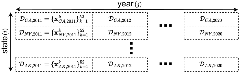
(a) An example of multiple time series data $\mathcal{D}_{i,j}$ (the U.S. flu dataset) where each year constitutes a period

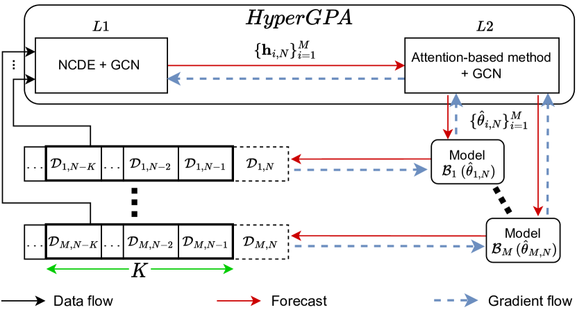
(b) Overall workflow of HyperGPA

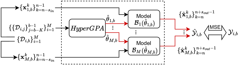
(c) Our training method

Figure 3. (a) An illustration of multiple time series data. (b) HyperGPA reads $K$ recent periods to generate target models’ parameters for the next period. (c) HyperGPA is trained by the MSE loss of target models in a seq-to-seq forecasting task.

3.2. Overall Workflow

We sketch our proposed method and introduce its step-by-step procedures as follows (cf. Fig. 3 (b)):

1. Let $\mathcal{D}_{input}=\{\{\mathcal{D}_{i,j}\}_{j=N-K}^{N-1}\}_{i=1}^{M}$ be the collected time series data for $K$ recent periods. The task of $\mathcal{B}_{i}$ is seq-to-seq forecasting in $\mathcal{D}_{i,N}$. In this situation, our hypernetwork forecasts the model parameters of $\{\mathcal{B}_{i}\}_{i=1}^{M}$, each of which is expected to work well for $\mathcal{D}_{i,N}$. One can consider that our task is a multi-task learning problem since there are $M$ similar tasks, i.e., forecasting the parameters for $M$ target models.

2. In short, HyperGPA can be expressed as $\{\hat{\boldsymbol{\theta}}_{i,N}\}_{i=1}^{M}$ $=L2(L1(\mathcal{D}_{input}),\mathbf{A})$, where $L1$ is a shared multi-task layer, and $L2$ is a parameter generating layer.

   1. $\{\mathbf{h}_{i,N}\}_{i=1}^{M}=L1(\mathcal{D}_{input})$. The shared multi-task layer reads the previous periods $\mathcal{D}_{input}$ and forecasts $\{\mathbf{h}_{i,N}\}_{i=1}^{M}$, the hidden representation of the next period $\{\mathcal{D}_{i,N}\}_{i=1}^{M}$. At this step, we utilize the adaptive graph convolutional (AGC) technique to discover latent relationships among those $M$ different correlated time series (Bai et al., 2020). Therefore, our method can be used even when the explicit relationships among $M$ time series are unknown, which significantly improves the applicability of our method. In order to simultaneously process $M$ time series data, we integrate AGC and NCDEs into a single framework.

   2. $\{\hat{\boldsymbol{\theta}}_{i,N}\}_{i=1}^{M}=L2(\{\mathbf{h}_{i,N}\}_{i=1}^{M},\mathbf{A})$. The parameter generating layer forecasts the parameters of each target model $\hat{\boldsymbol{\theta}}_{i,N}$ from the forecast characteristics of the future period $\mathbf{h}_{i,N}$. We use an attention-based parameter generation method. Also, GCNs are utilized to consider connections between different nodes (e.g., weight, bias) in the adjacency matrix of a computation graph $\mathbf{A}$.

3. With the $i$-th target model $\mathcal{B}_{i}$ equipped with the forecast parameters $\hat{\boldsymbol{\theta}}_{i,N}$, we perform the seq-to-seq forecasting task in $\mathcal{D}_{i,N}$.

3.3. $\boldsymbol{L1}$: Shared Multi-Task Layer

We first design a shared multi-task layer to discover underlying dynamics and forecast hidden representations $\{\mathbf{h}_{i,N}\}_{i=1}^{M}$ from past periods. The representation $\mathbf{h}_{i,N}$ contains the expected future period characteristics of $\mathcal{D}_{i,N}$, from which the next parameter generating layer forecasts the future model parameters $\hat{\boldsymbol{\theta}}_{i,N}$. If the forecast hidden representation is correct, i.e., if it represents the future period characteristics well, $\hat{\boldsymbol{\theta}}_{i,N}$ will also work well for the future period $\mathcal{D}_{i,N}$.

We use the following method to combine NCDEs and AGC into a single framework:

(1) $$\mathbf{h^{\prime}}_{i}(1) =\Gamma_{i}(\mathbf{x}_{i}(1);\boldsymbol{\theta}_{\Gamma_{i}}),$$

(2) $$\mathbf{h^{\prime}}_{i}(T) =\mathbf{h^{\prime}}_{i}(1)+\int_{1}^{T}G(\{\mathbf{h^{\prime}}_{i}(t)\}_{i=1}^{M};\boldsymbol{\theta}_{G})\mathrm{d}\mathbf{X}_{i}(t),$$

(3) $$\mathbf{h}_{i,N} =\mathbf{h^{\prime}}_{i}(T),$$

where $\mathbf{h^{\prime}}_{i}(t)$ is an NCDE hidden vector of the $i$-th time series at integral time $t$; and the final integral time $T$ is the total time length of input for recent periods, $\sum_{j=N-K}^{N-1}|\mathcal{D}_{i,j}|$— note that $T$ is the total number of observations because we assume regularly sampled time series (in general cases, we can set $T$ as the difference between the physical time of the first observation and that of the last observation in $\mathcal{D}_{input}$). $T$ should be the same for all $i$-th time series because they should evolve together with a graph function in NCDEs. In addition, $\{\mathbf{x}_{i}(1)\}_{i=1}^{M}$ are feature vectors at initial time in $\mathcal{D}_{input}$, and $\{\mathbf{X}_{i}(t)\}_{i=1}^{M}$ are interpolated lines of $\mathcal{D}_{input}$. Each $\Gamma_{i}$ maps the initial feature vector $\mathbf{x}_{i}(1)$ into the initial NCDE hidden vector $\mathbf{h^{\prime}}_{i}(1)$. Along the interpolated path, NCDEs generate the final NCDE hidden vector, $\mathbf{h^{\prime}}_{i}(T)$, which is $\mathbf{h}_{i,N}$. The important point to note is that $G$, which is shared by all $i$-th time series, includes an AGC function. Thus, all $i$-th time series are processed simultaneously through NCDEs and help each other to forecast the next hidden representation. We train the NCDE function with the adjoint method, so the space complexity for forward evaluations in NCDEs is constant.

3.4. $\boldsymbol{L2}$: Parameter Generating Layer

Given $\mathbf{h}_{i,N}$, we use an attention-based parameter generation method and GCNs to generate $\hat{\boldsymbol{\theta}}_{i,N}$:

(4) $$\{\mathbf{z}_{i,N}^{l}\}_{l=1}^{L} =\Phi(\mathbf{h}_{i,N};\boldsymbol{\theta}_{\Phi}),$$

(5) $$\{\mathbf{q}_{i,N}^{l}\}_{l=1}^{L} =\text{GCN}(\{\mathbf{z}_{i,N}\}_{l=1}^{L};\mathbf{A},\boldsymbol{\theta}_{\text{GCN}}),$$

(6) $$\mathbf{a}_{c,i,N}^{l} =Softmax_{c}(\mathbf{q}_{i,N}^{l}\boldsymbol{\theta}_{F}^{l}),$$

(7) $$\mathbf{\hat{\boldsymbol{\theta}}}_{i,N} =\{\sum_{c=1}^{C}\mathbf{a}_{c,i,N}^{l}\tilde{\boldsymbol{\theta}}_{c}^{l}\}_{l=1}^{L}.$$

For parameter generation, we use an attention-based method. In this method, there are query, keys, and values, like (Vaswani et al., 2017). Values are candidate parameters and each candidate has a key. $\mathbf{h}_{i,N}$ is mapped into query vectors. Because $\mathbf{h}_{i,N}$ includes the information of $\mathcal{D}_{i,N}$, query vectors should take the information of the period into account. Then, a generated target model $\mathbf{\hat{\boldsymbol{\theta}}}_{i,N}$ is the weighted sum of candidate parameters with attention coefficients from the key-query evaluation. (cf. Eq. 6 and 7)

$\mathbf{z}_{i,N}^{l}$, an initial query vector for the $l$-th parameter vertex $v_{l}$, is generated from $\mathbf{h}_{i,N}$ by a mapping function $\Phi$. Then, $\{\mathbf{z}_{i,N}^{l}\}_{l=1}^{L}$ are transformed into final query vectors $\{\mathbf{q}_{i,N}^{l}\}_{l=1}^{L}$, considering the connection of each node with the adjacency matrix of a computation graph $\mathbf{A}$ via GCNs. $Softmax_{c}$ denotes the $c$-th elements after the softmax operation. $\tilde{\boldsymbol{\theta}}_{c}^{l}$ is the $c$-th learnable candidate parameter for $v_{l}$, $C$ is the number of candidate parameters, and $\boldsymbol{\theta}_{F}^{l}\in\mathbb{R}^{dim(\mathbf{q})\times C}$ is a learnable key matrix. According to query-key evaluations, the attention coefficients of candidate parameters is determined. This approach has several advantages over a simple mapping method where $\mathbf{h}_{i,N}$ are directly converted into $\mathbf{\hat{\boldsymbol{\theta}}}_{i,N}$ through several linear layers. We will show the improvement in the attention-based method in Sec. 4.4.

One can use various graph networks, e.g., AGC, GAT (Veličković et al., 2018), and GCN (Kipf and Welling, 2017). In all experiments, we select GAT as the graph convolutional network of $L2$. This is because the experiments in Appendix B show that GAT is an reasonable choice although others sometimes produce better results than GAT.

3.5. Training Algorithm

Let $\{\{\mathcal{D}_{i,j}\}_{j=1}^{N-1}\}_{i=1}^{M}$ be the entire training time series data. We use the following procedures to train our hypernetwork (cf. Fig. 3 (c)):

1. We create several mini-batches $(\{\{\mathcal{D}_{i,j}\}_{j=b-K}^{b-1}\}_{i=1}^{M},$ $\{\mathcal{D}_{i,b}\}_{i=1}^{M})$, where $K+1\leq b\leq N-1$. Our hypernetwork reads $\{\{\mathcal{D}_{i,j}\}_{j=b-K}^{b-1}\}_{i=1}^{M}$ to generate the target model’s parameters and the loss is computed with the target model’s forecasting accuracy on $\{\mathcal{D}_{i,b}\}_{i=1}^{M}$. Given the range $[1,N-1]$, we can create multiple such mini-batches for training.

2. We feed $\{\{\mathcal{D}_{i,j}\}_{j=b-K}^{b-1}\}_{i=1}^{M}$ into our hypernetwork, which produces $\{\hat{\boldsymbol{\theta}}_{i,b}\}_{i=1}^{M}$. Each target model $\mathcal{B}_{i}$ equipped with $\hat{\boldsymbol{\theta}}_{i,b}$ performs a seq-to-seq forecasting task in $\mathcal{D}_{i,b}=\{\mathbf{x}_{i,b}^{k}\}_{k=1}^{|\mathcal{D}_{i,b}|}$. $\mathcal{B}_{i}$ reads $\{\mathbf{x}_{i,b}^{k}\}_{k=n-s_{in}}^{n-1}$ to forecast $\{\mathbf{x}_{i,b}^{k}\}_{k=n}^{n+s_{out}-1}$.

3. Let $\mathcal{Y}_{i,b}$ be the ground-truth for $\mathcal{B}_{i}$ and $\hat{\mathcal{Y}}_{i,b}$ be the forecasting results by $\mathcal{B}_{i}$ configured with $\hat{\boldsymbol{\theta}}_{i,b}$. Our training method lets the hypernetwork produce the best parameters, which leads to the smallest possible mean squared error (MSE), $MSE_{1}$, between the ground-truth $\{\mathcal{Y}_{i,b}\}_{i=1}^{M}$ and the inference $\{\hat{\mathcal{Y}}_{i,b}\}_{i=1}^{M}$.

4. Also, we train HyperGPA with another MSE, $MSE_{2}$, between $\{\mathcal{Y}_{i,b}\}_{i=1}^{M}$ and inference by a target model configured with $\{\tilde{\boldsymbol{\theta}}_{\hat{c}_{i,b}^{l}}^{l}\}_{l=1}^{L}$, where $\hat{c}_{i,b}^{l}=\operatorname*{argmax}\limits_{c}\mathbf{a}_{c,i,b}^{l}$. With $MSE_{2}$, each candidate becomes meaningful (i.e. forecasts well) in our task. The final loss is $MSE_{1}+\lambda MSE_{2}$ where $\lambda$ is the regularization coefficient of $MSE_{2}$.

4. EXPERIMENTS

We now evaluate HyperGPA on time series forecasting benchmarks. Our experiments are primarily designed to show how accurate our method is compared to other baselines. Specifically, we aim to answer the following research questions: RQ.1) How accurately does a target model generated by HyperGPA forecast future outcomes, compared to other baselines? RQ.2) How does the size of a target model affect the performance under two possible approaches: HyperGPA and a vanilla approach? RQ.3) How do various design choices of HyperGPA, e.g., the type of graph functions, influence the ability to forecast future parameters?

Table 2. MSE improvements w.r.t. Vanilla. Target models are in the typewriter font and baselines are in italics.

Target Model	Vanilla Training	Hypernetwork		Countermeasure for Temporal Drifts		HyperGPA
		HyperLSTM (GRU)	ANODEV2	RevIN	AdaLSTM (GRU)
LSTM	0%	-105.3%	N/A	-28.0%	-217.6%	64.1%
GRU	0%	-137.5%	N/A	-26.3%	-178.8%	45.5%
SeqToSeq(LSTM)	0%	-115.5%	N/A	-20.0%	N/A	59.1%
SeqToSeq(GRU)	0%	-131.3%	N/A	-26.3%	N/A	44.3%
ODERNN	0%	N/A	23.1%	-58.9%	N/A	63.8%
NCDE	0%	N/A	-139.7%	-41.1%	N/A	50.6%

Table 3. Experimental results. The best result for each target model is in boldface and for all target models with asterisk^∗.

Target Model	Generating/Training Method	Flu		Stock-US		Stock-China		USHCN
		MSE	PCC	MSE	PCC	MSE	PCC	MSE	PCC
LSTM	Vanilla	0.367±0.016	0.910±0.003	0.213±0.010	0.902±0.005	0.050±0.001	0.975±0.000	0.239±0.003	0.841±0.001
	HyperLSTM	0.582±0.019	0.852±0.005	0.751±0.103	0.605±0.071	0.103±0.007	0.949±0.003	0.249±0.004	0.824±0.003
	RevIN	0.506±0.097	0.917±0.010	0.063±0.001	0.966±0.000	0.049±0.002	0.977±0.001	0.589±0.015	0.693±0.009
	AdaLSTM	0.740±0.075	0.814±0.019	0.379±0.102	0.787±0.068	0.321±0.064	0.834±0.037	0.595±0.026	0.594±0.015
	HyperGPA	0.118±0.004	0.971±0.001∗	0.050±0.002	0.973±0.000∗	0.026±0.001	0.987±0.000	0.221±0.003	0.844±0.002∗
GRU	Vanilla	0.275±0.006	0.933±0.002	0.102±0.003	0.952±0.002	0.037±0.002	0.982±0.001	0.232±0.001	0.840±0.001
	HyperGRU	0.520±0.033	0.863±0.010	0.462±0.046	0.772±0.030	0.075±0.002	0.963±0.002	0.244±0.004	0.832±0.002
	RevIN	0.379±0.039	0.938±0.004	0.060±0.001	0.967±0.000	0.040±0.000	0.981±0.000	0.465±0.007	0.699±0.008
	AdaGRU	0.616±0.035	0.849±0.009	0.233±0.043	0.875±0.028	0.170±0.017	0.913±0.009	0.472±0.026	0.676±0.018
	HyperGPA	0.116±0.004∗	0.971±0.001∗	0.052±0.002	0.972±0.001	0.026±0.001	0.987±0.000	0.229±0.004	0.841±0.003
SeqToSeq (LSTM)	Vanilla	0.353±0.005	0.914±0.002	0.167±0.005	0.926±0.003	0.045±0.001	0.978±0.001	0.236±0.003	0.835±0.002
	HyperLSTM	0.559±0.021	0.855±0.007	0.643±0.084	0.674±0.052	0.097±0.045	0.952±0.023	0.243±0.004	0.826±0.003
	RevIN	0.345±0.021	0.944±0.004	0.061±0.001	0.967±0.000	0.044±0.002	0.979±0.001	0.585±0.014	0.682±0.016
	HyperGPA	0.128±0.006	0.969±0.001	0.048±0.001∗	0.973±0.001∗	0.026±0.001	0.987±0.000	0.220±0.007∗	0.843±0.002
SeqToSeq (GRU)	Vanilla	0.250±0.005	0.939±0.001	0.112±0.006	0.948±0.003	0.035±0.001	0.983±0.000	0.232±0.001	0.839±0.001
	HyperGRU	0.502±0.023	0.872±0.007	0.464±0.092	0.769±0.057	0.073±0.008	0.964±0.004	0.236±0.003	0.831±0.001
	RevIN	0.291±0.032	0.954±0.003	0.060±0.002	0.967±0.001	0.039±0.003	0.981±0.001	0.519±0.006	0.678±0.003
	HyperGPA	0.130±0.014	0.968±0.003	0.049±0.003	0.973±0.001∗	0.025±0.000∗	0.988±0.000∗	0.222±0.004	0.844±0.005∗
ODERNN	Vanilla	0.361±0.039	0.907±0.010	0.200±0.015	0.894±0.014	0.056±0.007	0.972±0.004	0.235±0.004	0.840±0.001
	ANODEV2	0.298±0.014	0.926±0.004	0.120±0.013	0.940±0.009	0.037±0.001	0.982±0.001	0.233±0.004	0.842±0.001
	RevIN	0.549±0.226	0.905±0.008	0.068±0.001	0.964±0.000	0.048±0.002	0.978±0.001	0.855±0.046	0.529±0.021
	HyperGPA	0.134±0.016	0.967±0.004	0.050±0.001	0.972±0.000	0.026±0.001	0.987±0.000	0.226±0.007	0.840±0.004
NCDE	Vanilla	0.387±0.042	0.900±0.011	0.130±0.015	0.929±0.007	0.040±0.001	0.980±0.001	0.234±0.004	0.829±0.002
	ANODEV2	0.821±0.011	0.778±0.004	0.244±0.002	0.850±0.001	0.141±0.001	0.929±0.001	0.483±0.002	0.616±0.001
	RevIN	0.439±0.022	0.919±0.003	0.060±0.001	0.967±0.000	0.040±0.001	0.981±0.000	0.713±0.008	0.467±0.015
	HyperGPA	0.167±0.020	0.959±0.004	0.049±0.002	0.973±0.001∗	0.027±0.001	0.987±0.001	0.227±0.004	0.837±0.003

4.1. Experimental Setup

Datasets. We evaluate our approach on four popular time series forecasting benchmarks ranging from pandemic and stock to climate forecasting datasets: Flu, Stock-US, Stock-China, and USHCN. These are all popular benchmark datasets. Refer to Appendix C.1 for their detailed descriptions, including the configurations of the temporal window sizes, $s_{in}$ and $s_{out}$ in each dataset. In our evaluations for all these datasets, we use the last and the second to the last window as a test and a validation set, respectively.

Target Models & Baselines. We first explain the difference between a target model and a baseline. The target model is a time series model which performs a seq-to-seq forecasting task. On the other hand, the baseline is a way to generate or train the target model’s parameters as done in HyperGPA.

For target models, we use six time series models, ranging from RNN to NODE and NCDE-based models. For RNNs, we use LSTM and GRU (Hochreiter and Schmidhuber, 1997; Cho et al., 2014). Because the task of a target model is to read a sequence and forecast its next sequence, we also use a seq-to-seq learning model (SeqToSeq) as a target model (Sutskever et al., 2014) — note that this model can be based on either LSTM or GRU. In addition, we use a latent ODE model, ODERNN (Rubanova et al., 2019), and an NCDE-based model, NCDE (Kidger et al., 2020).

For baselines, there are 3 categories: i) In a vanilla method, one can directly train the parameters of a target model with recent data. There are neither hypernetworks nor approaches addressing temporal drifts. Target models trained this way is denoted by Vanilla (cf. Fig. 2). ii) There are two hypernetwork-based methods. HyperLSTM or HyperGRU (Ha et al., 2016), depending on the underlying cell types, can be applied to RNN-based models only, i.e., LSTM, GRU, SeqToSeq(LSTM), and SeqToSeq(GRU). Also, ANODEV2 (Zhang et al., 2019) is a hypernetwork for NODEs that can be applied to NODE variants only (i.e., ODERNN and NCDE). iii) RevIN (Kim et al., 2022), AdaLSTM, and AdaGRU (Du et al., 2021) are designed to address the temporal drifts. RevIN can be used for various time series forecasting models, whereas AdaLSTM and AdaGRU are for LSTM and GRU only, respectively. Additionally, there is a traditional statistical model, ARIMA (Hillmer and Tiao, 1982). However, we include its results only in an appendix, because ARIMA has the worst score overall. All baselines are trained separately for each target model, whereas our method, which internally has a shared multi-task layer, is trained collectively and generates multiple target models’ parameters simultaneously.

Hyperparameters. We have two key hyperparameters for the target models, a hidden size and the number of layers. The hidden size is in $\{16,32,64\}$ and the number of layers is in $\{1,2,3\}$. We use the same settings for the baselines. However, for HyperGPA, we fix their hidden size and the number of layers to $16$ and $1$ respectively, which leads to the smallest target model size — surprisingly, the smallest setting can also produce the best forecasting outcomes in many cases of our experiments, which shows the efficacy of our design. This is related to another advantage of HyperGPA which will be described in Sec. 4.3 (RQ.2). Refer to Appendix C.2 for detailed hyperparameter configurations.

Metrics. We train HyperGPA and the baselines with MSE — the validation metric is also MSE. For testing, we use the pearson correlation coefficient (PCC) and MSE. We run 5 times for each evaluation case and report their mean and standard deviation (std. dev.) values.

4.2. RQ.1: Time Series Forecasting Accuracy

Table 2 shows the summary evaluation results which contain the improvement ratio of the baselines and HyperGPA over Vanilla in MSE, i.e., $\frac{\textit{Vanilla's}\ \text{MSE}-\textit{HyperGPA(or baseline)'s}\ \text{MSE}}{\textit{Vanilla's}\ \text{MSE}}$. We average the ratio values across all datasets. Table 3 shows detailed experimental results. Also, there are visualizations. Fig. 4 (a) shows forecast lines, and Fig. 4 (b) shows MSE values over time. We refer the reader to Appendix D for full experimental results with all evaluation metrics, and Appendix E for full visualizations.

Summary. HyperLSTM/GRU shows worse scores than those by Vanilla. In all cases, they fail to increase the model accuracy. For ODERNN, ANODEV2 achieves better scores than those of Vanilla but not for NCDE. One possible reason is that ANODEV2 was originally designed for NODEs only.

In the baseline approaches addressing temporal drifts, AdaLSTM/GRU fails to address temporal drifts. We think that this is because the temporal drifts of the experimental datasets are too large for this approach to overcome, as in Fig. 4 (a). Also, RevIN has poor performance inferior to Vanilla. However, in spite of the poor summary scores, RevIN is still an effective method for temporal drifts. We show relevant results in the following detailed result paragraphs.

Our model, HyperGPA, consistently outperforms all baselines for all target models. Especially for LSTM and ODERNN, there are about 60% improvements, proving the efficacy of the proposed method.

Detail (Flu). In Table 3, among the baselines, except for ANODEV2 in ODERNN, all baselines are worse than Vanilla in terms of MSE. However, when checking PCC and the visualization in Fig. 4 (a), RevIN alleviates the temporal drift problem to some extent. RevIN catches a changed dynamics more accurately in Fig. 4 (a), and achieves a higher PCC than Vanilla in Table 3.

Although RevIN alleviates temporal drifts, it has worse MSE scores. We think that in RevIN, target models do not consider the data magnitude because of the normalization, and when the data magnitude is drastically changing, the target models become unstable. The unstable forecasting visualization can be checked in Fig. 4 (a) around $t\approx 460$ or $500$.

Meanwhile, our HyperGPA outperforms others in almost all cases, and achieves the lowest MSE. In Fig. 4 (a), HyperGPA forecasts the changed dynamics almost exactly. Also, HyperGPA performs better in all types of the target model, which shows the adaptiveness of our method.

Detail (Stock). Among baselines, in the two stock datasets, RevIN mostly shows the lowest MSE scores in Fig. 4 (b) over time, which leads to improvement over Vanilla in Table 3. We observe that RevIN is helpful for temporal drifts in the two datasets. However, HyperGPA attains more enhanced performance in all aspects, showing better evaluation scores in Table. 3 and Fig. 4 (b).

Detail (USHCN). HyperGPA achieves the best scores in almost all cases, whereas there is no improvement in other baselines, compared to Vanilla, except for ANODEV2 in ODERNN. Even RevIN shows poor performance. These results in all datasets show that HyperGPA can successfully generate the parameters of all target models which work well in the future.

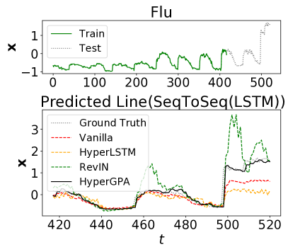
(a) Data: Flu, Target Model: SeqToSeq (LSTM)

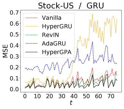
(b) Stock-US, GRU

Figure 4. (a) Forecast lines of various methods. The upper figure shows a train and test line. A validation line is included in the test line. The lower figure shows the predicted line of baselines and HyperGPA. (b) MSE over time in various methods.

4.3. RQ.2: Accuracy by Varying Target Model Size

We compare Vanilla and HyperGPA, varying the hidden size of target models from 8 to 256 — the larger the hidden size, the larger the target model size. As in Fig. 5, HyperGPA shows stable errors regardless of the hidden size of a target model whereas Vanilla does not show reliable forecasting accuracy when the target model size is small. This result shows that we can use small target models with HyperGPA, which drastically reduces the overheads for maintaining target models in practice.

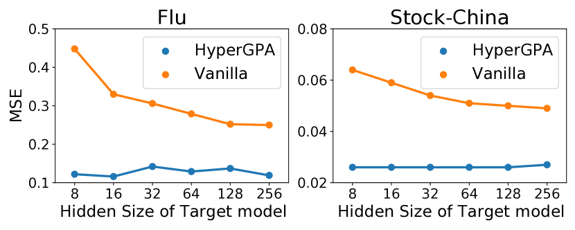
Figure 5. Sensitivity to the hidden size of the two target models, GRU(Flu), and LSTM(Stock-China)

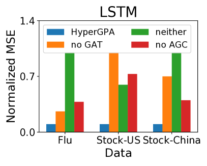
(a) Ablation w.r.t. using GCNs or not

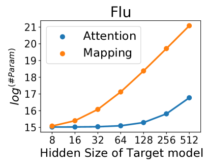
(b) The required model size of HyperGPA vs. the hidden size of target models

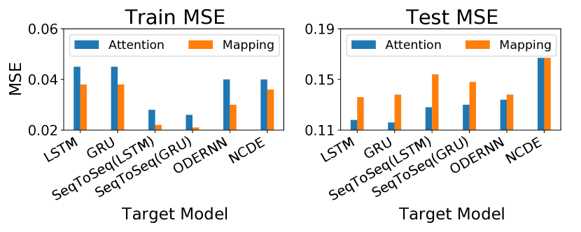
(c) Train and test MSE of the two possible parameter generation methods in Flu. ‘Attention’ means our full model.

Figure 6. Experiments for an design choice

4.4. RQ.3: Ablation Studies

We justify our specific design choices for HyperGPA. Refer to Appendix B for experiments on other design choices.

With or Without Graph Function. In order to define two ablation models, we remove AGC from $L1$ (Eq. (2)) or GAT from $L2$ (Eq. (5)) — note that we use GAT as the graph convolution function of $L2$. Fig. 6 (a) shows MSE for each case where the target model is LSTM. HyperGPA denotes our full model; neither means our model without AGC or GAT. The normalized MSE is used for fair comparison. In almost all cases, HyperGPA shows the lowest errors. Higher errors of no AGC show that considering different correlated time series simultaneously helps HyperGPA to better discover underlying dynamics. Also, no GAT has worse results, which means that the information of a computation graph is needed for generating reliable parameters. As such, we conclude that both the computation graph of a target model and the correlation between multiple time series are helpful for accurate model parameter generations.

Attention-Based Method or Simple Mapping Method. Fig. 6 (b) and (c) show the advantages of our attention-based parameter generation method in Sec. 3.4, compared to the simple mapping method where $\mathbf{h}_{i,N}$ are directly mapped into the parameters of a target model through linear layers. According to Fig. 6 (b), as the hidden size of target models increases, the required number of parameters of HyperGPA increases more rapidly in the simple mapping method than in the attention-based method. In addition, our attention-based method is more robust to overfitting as in Fig. 6 (c).

5. CONCLUSION

We presented a novel approach to defend against the temporal drift by designing a hypernetwork generating the future parameters of a target model. Our hypernetwork, called HyperGPA, is model-agnostic as our experiments showed that it works well for all the tested target models and marks the best accuracy in most cases. In addition, we showed that with HyperGPA, small target models are sufficient to be used in real-world applications (if their parameters are carefully configured by our method), which drastically reduces the maintenance overhead of target models.

Limitations. Because HyperGPA is based on NCDEs which are unknown for their accuracy for long time series, we will further extend our research towards it.

Societal Impacts. Our method can enhance time series forecasting which has many real-world applications, e.g., forecasting stock prices, weather conditions, etc. In addition, we showed that our method results in using small target models, which reduce carbon emissions during inference. Because our main contribution is to improve forecasting performances under temporal drifts, we think HyperGPA has no significant negative impact.

Appendix A HYPERGRU

We define HyperGRU since only HyperLSTM is defined in (Ha et al., 2016). Let $\mathbf{x}_{t}$ be a time series observation at time $t$. GRU (Cho et al., 2014) is defined as follows:

(8) $$\mathbf{r}_{t} =\sigma(W^{\mathbf{r}}_{\mathbf{x}}\mathbf{x}_{t}+W^{\mathbf{r}}_{\mathbf{h}}\mathbf{h}_{t-1}+b^{\mathbf{r}}),$$

(9) $$\mathbf{z}_{t} =\sigma(W^{\mathbf{z}}_{\mathbf{x}}\mathbf{x}_{t}+W^{\mathbf{z}}_{\mathbf{h}}\mathbf{h}_{t-1}+b^{\mathbf{z}}),$$

(10) $$\mathbf{g}_{t} =\delta(W^{\mathbf{g}}_{\mathbf{x}}\mathbf{x}_{t}+\mathbf{r}_{t}\odot W^{\mathbf{g}}_{\mathbf{h}}\mathbf{h}_{t-1}+b^{\mathbf{g}}),$$

(11) $$\mathbf{h}_{t} =(1-\mathbf{z}_{t})\odot\mathbf{g}_{t}+\mathbf{z}_{t}\odot\mathbf{h}_{t-1},$$

where $\sigma$ is a sigmoid function, $\delta$ is a hyperbolic tangent function, and $\odot$ is an element-wise multiplication. Likewise, HyperGRU is defined as follows:

(12) $$\hat{\mathbf{x}}_{t} =\mathbf{x}_{t}\oplus\mathbf{h}_{t-1},$$

(13) $$\hat{\mathbf{r}}_{t} =\sigma(LN(W^{\hat{\mathbf{r}}}_{\hat{\mathbf{x}}}\hat{\mathbf{x}}_{t}+W^{\hat{\mathbf{r}}}_{\hat{\mathbf{h}}}\hat{\mathbf{h}}_{t-1}+b^{\hat{\mathbf{r}}})),$$

(14) $$\hat{\mathbf{z}}_{t} =\sigma(LN(W^{\hat{\mathbf{z}}}_{\hat{\mathbf{x}}}\hat{\mathbf{x}}_{t}+W^{\hat{\mathbf{z}}}_{\hat{\mathbf{h}}}\hat{\mathbf{h}}_{t-1}+b^{\hat{\mathbf{z}}})),$$

(15) $$\hat{\mathbf{g}}_{t} =\delta(LN(W^{\hat{\mathbf{g}}}_{\hat{\mathbf{x}}}\hat{\mathbf{x}}_{t}+\hat{\mathbf{r}}_{t}\odot W^{\hat{\mathbf{g}}}_{\hat{\mathbf{h}}}\hat{\mathbf{h}}_{t-1}+b^{\hat{\mathbf{g}}})),$$

(16) $$\hat{\mathbf{h}}_{t} =(1-\hat{\mathbf{z}}_{t})\odot\hat{\mathbf{g}}_{t}+\hat{\mathbf{z}}_{t}\odot\hat{\mathbf{h}}_{t-1},$$

where $\oplus$ means a concatenation. From $\hat{\mathbf{h}}_{t}$, the embeddings of each gate $\mathbf{a}^{\mathbf{h},y}_{t},\mathbf{a}^{\mathbf{x},y}_{t},\mathbf{a}^{\mathbf{b},y}_{t}$ are generated, where $y\in\{\mathbf{r},\mathbf{z},\mathbf{g}\}$. In addition, those embeddings are transformed into $\mathbf{d}^{\mathbf{h},y}_{t},\mathbf{d}^{\mathbf{x},y}_{t},\mathbf{d}^{\mathbf{b},y}_{t}$:

(17) $$\mathbf{a}^{\mathbf{h},y}_{t} =W_{\hat{\mathbf{h}}}^{\mathbf{h},y}\hat{\mathbf{h}}_{t-1}+b_{\hat{\mathbf{h}}}^{\mathbf{h},y},$$

(18) $$\mathbf{a}^{\mathbf{x},y}_{t} =W_{\hat{\mathbf{h}}}^{\mathbf{x},y}\hat{\mathbf{h}}_{t-1}+b_{\hat{\mathbf{h}}}^{\mathbf{x},y},$$

(19) $$\mathbf{a}^{\mathbf{b},y}_{t} =W_{\hat{\mathbf{h}}}^{\mathbf{b},y}\hat{\mathbf{h}}_{t-1}+b_{\hat{\mathbf{h}}}^{\mathbf{b},y},$$

(20) $$\mathbf{d}^{\mathbf{h},y}_{t} =W_{\mathbf{a}}^{\mathbf{h},y}\mathbf{a}^{\mathbf{h},y}_{t}+b_{\mathbf{a}}^{\mathbf{h},y},$$

(21) $$\mathbf{d}^{\mathbf{x},y}_{t} =W_{\mathbf{a}}^{\mathbf{x},y}\mathbf{a}^{\mathbf{x},y}_{t}+b_{\mathbf{a}}^{\mathbf{x},y},$$

(22) $$\mathbf{d}^{\mathbf{b},y}_{t} =W_{\mathbf{a}}^{\mathbf{b},y}\mathbf{a}^{\mathbf{b},y}_{t}+b_{\mathbf{a}}^{\mathbf{b},y}.$$

Finally, $\mathbf{d}^{\mathbf{h},y}_{t},\mathbf{d}^{\mathbf{x},y}_{t},\mathbf{d}^{\mathbf{b},y}_{t}$ adjust the parameters of the main GRU and $h_{t}$ is generated:

(23) $$\mathbf{r}_{t} =\sigma(LN(\mathbf{d}^{\mathbf{x},\mathbf{r}}_{t}\odot W^{\mathbf{r}}_{\mathbf{x}}\mathbf{x}_{t}+\mathbf{d}^{\mathbf{h},\mathbf{r}}_{t}\odot W^{\mathbf{r}}_{\mathbf{h}}\mathbf{h}_{t-1}+\mathbf{d}^{\mathbf{b},\mathbf{r}}_{t})),$$

(24) $$\mathbf{z}_{t} =\sigma(LN(\mathbf{d}^{\mathbf{x},\mathbf{z}}_{t}\odot W^{\mathbf{z}}_{\mathbf{x}}\mathbf{x}_{t}+\mathbf{d}^{\mathbf{h},\mathbf{z}}_{t}\odot W^{\mathbf{z}}_{\mathbf{h}}\mathbf{h}_{t-1}+\mathbf{d}^{\mathbf{b},\mathbf{z}}_{t})),$$

(25) $$\mathbf{g}_{t} =\delta(LN(\mathbf{d}^{\mathbf{x},\mathbf{g}}_{t}\odot W^{\mathbf{g}}_{\mathbf{x}}\mathbf{x}_{t}+\mathbf{r}_{t}\odot\mathbf{d}^{\mathbf{h},\mathbf{g}}_{t}\odot W^{\mathbf{g}}_{\mathbf{h}}\mathbf{h}_{t-1}+\mathbf{d}^{\mathbf{b},\mathbf{g}}_{t})),$$

(26) $$\mathbf{h}_{t} =(1-\mathbf{z}_{t})\odot\mathbf{g}_{t}+\mathbf{z}_{t}\odot\mathbf{h}_{t-1}.$$

Appendix B ADDITIONAL DESIGN CHOICE

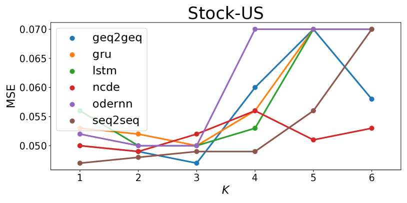
Figure 7. Sensitivity to the input period size $K$

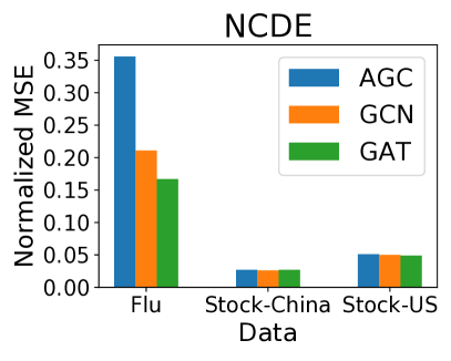
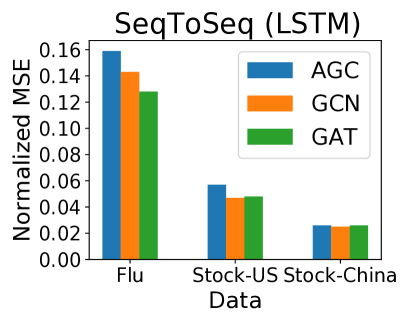
Figure 8. Changing the type of graph functions on the parameter generating layer ($L2$)

Period size $K$. Fig. 8 shows sensitivity analyses w.r.t. the input period size $K$. As shown, $K\leq 3$ produces the best outcomes. Feeding too much information leads to sub-optimal outcomes. For this reason, we use 2 or 3 as $K$.

The type of graph function in $L2$. Fig. 8 shows the results by varying the graph function of the parameter generating layer ($L2$) in Eq. (5). In addition to our choice of GAT, we test with a graph convolutional network (GCN) (Kipf and Welling, 2017) and an adaptive graph convolutional network (AGC) (Bai et al., 2020). In most cases, GAT and GCN show reasonable performance. On the other hand, AGC, which does not use the computation graph but learns its own virtual graph, sometimes shows the worst performance — note that, however, AGC is effective for the shared multi-task layer.

Appendix C REPRODUCIBILITY

We implement HyperGPA with Python v3.7 and PyTorch v1.8 and run our experiments on a machine equipped with Nvidia RTX Titan or 3090.

C.1. Datasets

Flu contains the number of flu patients, total patients, and providers who give information about patients, in each of the 51 U.S. states, collected weekly by the Centers for Disease Control and Prevention (CDC, 1946), i.e., $\dim(\mathbf{x})=3$. The data collection period is 2011–2020. In HyperGPA, we set the length of one window $\mathcal{D}_{i,j}$ to a year; the length is 52 (or 53) weeks. For Flu, each target time series model $\mathcal{B}_{i}$ reads recent $s_{in}=10$ observations and forecasts next $s_{out}=2$ observations.

We also use the daily historical stock prices of the U.S. and China (Stock-US and Stock-China) collected by (Investing.com, 2007) over 20 months. Each dataset contains the opening, closing, highest, and lowest stock prices per day, i.e., $\dim(\mathbf{x})=4$. We choose the top-30 companies with the highest market capitalization. For those two datasets, we set the window length to two months. Note that the stock prices for those companies are interconnected, i.e., they are loosely-coupled data. $s_{in}$ and $s_{out}$ for stock datasets are 10 and 4, respectively.

USHCN is a climate dataset that contains monthly average, minimum, and maximum temperature and precipitation in the U.S. states from the U.S. historical climatology network (USHCN, 1987), i.e., $\dim(\mathbf{x})=4$. The collection period is 1981–2012. The length of one window is a year, 12 months. We set $s_{in}$ and $s_{out}$ to 10 and 2.

After making the input and output pairs of target models like Step 2 in Sec. 3.5, Flu has 20K training pairs, 3K validation pairs, and 3K test pairs. Both Stock-US and Stock-China have 10K training pairs, 1K validation pairs, and 1K test pairs. USHCN has 17K training pairs, 0.5K validation pairs, and 0.5K test pairs.

C.2. Hyperparameters

We note that the hyperparameters of the target models (the number of layer, $n_{\mathcal{B}}$ and hidden size of target model, $\dim(\mathbf{h}_{\mathcal{B}})$) are already described in the main paper. In this section, we show the best hyperparameters for our baselines for reproducibility in Tables 5 to 10.

C.2.1. Baselines

For our baselines, we set the learning rate to $10^{-3}$ and the coefficient of $L_{2}$ regularization term to $10^{-5}$. The size of mini-batch is 256. For Vanilla, there is no additional hyperparameter. For HyperLSTM/GRU, there are 2 additional hyperparameters, $\dim(\hat{\mathbf{h}})$ and $\dim(\mathbf{a})$, that are the dimensionality of $\hat{\mathbf{h}}$ and $\mathbf{a}$, defined in (Ha et al., 2016) or Appendix A. As $\dim(\mathbf{a})<\dim(\hat{\mathbf{h}})<\dim(\mathbf{h}_{\mathcal{B}})$ recommended in (Ha et al., 2016), $\dim(\hat{\mathbf{h}})$ is in $\{32,16,8\}$, and $\dim(\mathbf{a})$ is in $\{16,8,4\}$. For ANODEV2, we configure the baseline as in (Zhang et al., 2019) and RevIN is just adding an adaptation layer, so additional hyperparameters are not needed. AdaGRU/LSTM has an additional hyperparameter, $\lambda$ which is the coefficient of a drift-related loss. In an ARIMA case, there are 3 hyperparameters. $p,d,$ and $q$ denote the autoregressive, differences, and moving average components, respectively. $p$ is in {1,2,3}, $d$ in {0,1,2}, $q$ in {1,2,3}.

C.2.2. HyperGPA

For HyperGPA, the learning rate is set to $10^{-2}$, the coefficient of $L_{2}$ regularization term to $10^{-6}$, and the size of mini-batch to $10^{4}$. The reason why the size of the mini-batch for HyperGPA is much larger than that for the baselines is that i) HyperGPA generates the parameters of all target models, and ii) all target models are trained simultaneously. Because there are about 30 to 50 target models, the size of mini-batch for one target model is about 256. Each of $\dim(\mathbf{h}_{\mathcal{B}})$ and $n_{\mathcal{B}}$ in HyperGPA is set to 16 and 1, respectively.

The hidden size and the number of layers for $\Gamma$ in Eq. 1 are set to 32 and 2, respectively. The hidden size of NCDEs, $\dim(\mathbf{h^{\prime}})$ in Eq. (2), is in $\{32,64,128\}$. In AGC function, the node embedding size and the output size are set to 32. $\Phi$ is a one-layer fully connected layer without bias. The size of initial query vectors in Eq. 4, $\dim(\mathbf{z})$, is in $\{512,1024,2048\}$. In Eq. (5), GAT has three hyperparameters: i) number of heads, ii) depth, and iii) hidden size. The number of heads is set to 4, the depth to 3, and the hidden size to 128. In an attention-based generation method, the number of candidates model $C$ is in $\{3,5,10,20,48\}$, and the regularization coefficient of $MSE_{2}$, $\lambda$, is in $\{0,0.1,0.01\}$. For input window size $K$, we use $K=2$ in Flu, Stock-China, and Stock-China, and $K=3$ in USHCN.

Table 4. Hyperparameters for HyperGPA

Data	Target Model	$\dim(\mathbf{h^{\prime}})$	$\dim(\mathbf{z})$	$C$	$\lambda$
Flu	LSTM	128	2048	3	0.1
	GRU	128	1024	3	0.01
	SeqToSeq(LSTM)	128	1024	10	0.1
	SeqToSeq(GRU)	128	2048	3	0.01
	ODERNN	128	2048	10	0.0
	NCDE	128	512	3	0.1
Stock-US	LSTM	128	512	3	0.0
	GRU	128	512	10	0.01
	SeqToSeq(LSTM)	128	512	3	0.1
	SeqToSeq(GRU)	128	1024	5	0.0
	ODERNN	128	512	10	0.01
	NCDE	128	512	10	0.0
Stock-China	LSTM	128	512	3	0.1
	GRU	128	512	10	0.0
	SeqToSeq(LSTM)	128	2048	5	0.1
	SeqToSeq(GRU)	128	512	3	0.01
	ODERNN	128	1024	3	0.0
	NCDE	128	1024	5	0.0
USHCN	LSTM	128	512	48	0.01
	GRU	32	512	48	0.1
	SeqToSeq(LSTM)	32	512	48	0.01
	SeqToSeq(GRU)	128	512	48	0.1
	ODERNN	64	512	48	0.1
	NCDE	32	512	48	0.01

Table 5. Hyperparameters for Vanilla

Data	Target Model	$\dim(\mathbf{h}_{\mathcal{B}})$	$n_{\mathcal{B}}$
Flu	LSTM	64	1
	GRU	64	1
	SeqToSeq (LSTM)	64	1
	SeqToSeq (GRU)	64	1
	ODERNN	32	1
	NCDE	32	3
Stock-US	LSTM	64	1
	GRU	64	1
	SeqToSeq (LSTM)	64	1
	SeqToSeq (GRU)	64	1
	ODERNN	64	3
	NCDE	16	2
Stock-China	LSTM	64	1
	GRU	16	1
	SeqToSeq (LSTM)	64	1
	SeqToSeq (GRU)	64	1
	ODERNN	32	1
	NCDE	64	2
USHCN	LSTM	32	1
	GRU	16	1
	SeqToSeq (LSTM)	16	1
	SeqToSeq (GRU)	32	1
	ODERNN	64	2
	NCDE	32	3

Table 6. Hyperparameters for HyperLSTM/GRU

Data	Target Model	$\dim(\mathbf{h}_{\mathcal{B}})$	$n_{\mathcal{B}}$	$\dim(\mathbf{a})$	$\dim(\hat{\mathbf{h}})$
Flu	LSTM	64	1	16	8
	GRU	32	1	8	8
	SeqToSeq (LSTM)	64	1	4	8
	SeqToSeq (GRU)	16	1	4	16
Stock-US	LSTM	32	1	4	16
	GRU	16	1	16	8
	SeqToSeq (LSTM)	32	1	8	8
	SeqToSeq (GRU)	64	1	4	8
Stock-China	LSTM	16	1	4	8
	GRU	16	1	4	8
	SeqToSeq (LSTM)	16	1	4	8
	SeqToSeq (GRU)	32	1	4	8
USHCN	LSTM	32	1	4	16
	GRU	64	1	4	8
	SeqToSeq (LSTM)	64	1	4	32
	SeqToSeq (GRU)	64	1	4	8

Table 7. Hyperparameters for RevIN

Data	Target Model	$\dim(\mathbf{h}_{\mathcal{B}})$	$n_{\mathcal{B}}$
Flu	LSTM	16	3
	GRU	16	2
	SeqToSeq (LSTM)	16	1
	SeqToSeq (GRU)	32	1
	ODERNN	32	3
	NCDE	64	3
Stock-US	LSTM	16	1
	GRU	16	1
	SeqToSeq (LSTM)	16	1
	SeqToSeq (GRU)	16	1
	ODERNN	32	2
	NCDE	16	3
Stock-China	LSTM	32	1
	GRU	16	2
	SeqToSeq (LSTM)	16	1
	SeqToSeq (GRU)	16	1
	ODERNN	64	3
	NCDE	32	3
USHCN	LSTM	32	1
	GRU	16	3
	SeqToSeq (LSTM)	64	1
	SeqToSeq (GRU)	32	3
	ODERNN	64	2
	NCDE	64	3

Table 8. Hyperparameters for ANODEV2

Data	Target Model	$\dim(\mathbf{h}_{\mathcal{B}})$	$n_{\mathcal{B}}$
Flu	ODERNN	64	3
	NCDE	16	3
Stock-US	ODERNN	64	3
	NCDE	64	3
Stock-China	ODERNN	64	2
	NCDE	16	2
USHCN	ODERNN	64	3
	NCDE	32	3

Table 9. Hyperparameters for AdaLSTM/GRU

Data	Target Model	$\dim(\mathbf{h}_{\mathcal{B}})$	$n_{\mathcal{B}}$	$\lambda$
Flu	LSTM	64	1	1.0
	GRU	64	1	1.0
Stock-US	LSTM	64	1	1.0
	GRU	64	1	1.0
Stock-China	LSTM	64	1	1.0
	GRU	64	1	0.5
USHCN	LSTM	64	1	1.0
	GRU	32	1	1.0

Table 10. Hyperparameters for ARIMA

Data	$p$	$d$	$q$
Flu	2	1	1
Stock-US	1	1	2
Stock-China	1	1	1
USHCN	1	1	2

Appendix D FULL EXPERIMENTAL RESULTS

Full experimental results are shown from Table. 11 to Table. 14. Val.MSE is the MSE value in validation data, which is the criterion for selecting the best models.

Table 11. Experimental results for Flu

Target Model	Generation Way	Val.MSE	PCC	$R^{2}$	Exp.	MSE	MAE
ARIMA		0.502±0.000	0.695±0.000	0.152±0.000	0.168±0.000	1.091±0.000	0.579±0.000
LSTM	Vanilla	0.174±0.004	0.910±0.003	0.718±0.023	0.730±0.021	0.367±0.016	0.299±0.008
	HyperLSTM	0.236±0.008	0.852±0.005	0.434±0.038	0.471±0.032	0.582±0.019	0.388±0.010
	RevIN	0.230±0.022	0.917±0.010	0.842±0.017	0.844±0.018	0.506±0.097	0.256±0.007
	AdaLSTM	0.516±0.047	0.814±0.019	0.367±0.099	0.478±0.075	0.740±0.075	0.552±0.036
	HyperGPA	0.068±0.002	0.971±0.001	0.933±0.003	0.933±0.004	0.118±0.004	0.141±0.002
GRU	Vanilla	0.130±0.003	0.933±0.002	0.807±0.006	0.813±0.006	0.275±0.006	0.250±0.003
	HyperGRU	0.207±0.016	0.863±0.010	0.585±0.035	0.601±0.035	0.520±0.033	0.361±0.011
	RevIN	0.199±0.015	0.938±0.004	0.880±0.007	0.881±0.008	0.379±0.039	0.226±0.007
	AdaGRU	0.405±0.031	0.849±0.009	0.542±0.048	0.613±0.056	0.616±0.035	0.510±0.018
	HyperGPA	0.066±0.002	0.971±0.001	0.938±0.003	0.939±0.003	0.116±0.004	0.140±0.003
SeqToSeq(LSTM)	Vanilla	0.151±0.003	0.914±0.002	0.733±0.004	0.747±0.004	0.353±0.005	0.290±0.004
	HyperLSTM	0.211±0.015	0.855±0.007	0.502±0.035	0.527±0.032	0.559±0.021	0.372±0.007
	RevIN	0.193±0.007	0.944±0.004	0.888±0.006	0.890±0.006	0.345±0.021	0.219±0.005
	HyperGPA	0.070±0.004	0.969±0.001	0.932±0.006	0.932±0.006	0.128±0.006	0.143±0.004
SeqToSeq(GRU)	Vanilla	0.114±0.004	0.939±0.001	0.828±0.006	0.834±0.005	0.250±0.005	0.237±0.004
	HyperGRU	0.191±0.008	0.872±0.007	0.574±0.028	0.592±0.028	0.502±0.023	0.347±0.009
	RevIN	0.189±0.010	0.954±0.003	0.905±0.006	0.908±0.006	0.291±0.032	0.204±0.005
	HyperGPA	0.066±0.002	0.968±0.003	0.926±0.012	0.926±0.012	0.130±0.014	0.142±0.004
ODERNN	Vanilla	0.163±0.011	0.907±0.010	0.761±0.030	0.767±0.027	0.361±0.039	0.301±0.017
	ANODEV2	0.139±0.003	0.926±0.004	0.790±0.007	0.796±0.007	0.298±0.014	0.256±0.009
	RevIN	0.272±0.004	0.905±0.008	0.817±0.011	0.820±0.011	0.549±0.226	0.266±0.014
	HyperGPA	0.075±0.003	0.967±0.004	0.931±0.007	0.932±0.007	0.134±0.016	0.145±0.004
NCDE	Vanilla	0.137±0.019	0.900±0.011	0.775±0.015	0.781±0.016	0.387±0.042	0.296±0.011
	ANODEV2	0.457±0.002	0.778±0.004	0.041±0.017	0.077±0.018	0.821±0.011	0.480±0.005
	RevIN	0.259±0.012	0.919±0.003	0.843±0.005	0.848±0.005	0.439±0.022	0.251±0.004
	HyperGPA	0.071±0.003	0.959±0.004	0.913±0.009	0.914±0.009	0.167±0.020	0.164±0.008

Table 12. Experimental results for Stock-US

Target Model	Generation Way	Val.MSE	PCC	$R^{2}$	Exp.	MSE	MAE
ARIMA		0.205±0.000	0.548±0.000	-0.781±0.000	-0.748±0.000	0.620±0.000	0.609±0.000
LSTM	Vanilla	0.051±0.001	0.902±0.005	0.569±0.029	0.641±0.022	0.213±0.010	0.307±0.006
	HyperLSTM	0.089±0.005	0.605±0.071	-1.045±0.340	-0.491±0.248	0.751±0.103	0.586±0.038
	RevIN	0.045±0.000	0.966±0.000	0.930±0.000	0.933±0.000	0.063±0.001	0.183±0.001
	AdaLSTM	0.257±0.017	0.787±0.068	0.400±0.231	0.475±0.209	0.379±0.102	0.483±0.062
	HyperGPA	0.034±0.000	0.973±0.000	0.930±0.005	0.933±0.004	0.050±0.002	0.161±0.004
GRU	Vanilla	0.043±0.001	0.952±0.002	0.830±0.007	0.848±0.006	0.102±0.003	0.226±0.004
	HyperGRU	0.073±0.007	0.772±0.030	-0.167±0.113	0.103±0.086	0.462±0.046	0.453±0.015
	RevIN	0.044±0.000	0.967±0.000	0.933±0.001	0.935±0.000	0.060±0.001	0.178±0.000
	AdaGRU	0.176±0.021	0.875±0.028	0.645±0.073	0.693±0.073	0.233±0.043	0.377±0.045
	HyperGPA	0.034±0.000	0.972±0.001	0.927±0.005	0.930±0.004	0.052±0.002	0.164±0.004
SeqToSeq(LSTM)	Vanilla	0.042±0.001	0.926±0.003	0.688±0.014	0.744±0.011	0.167±0.005	0.274±0.004
	HyperLSTM	0.077±0.004	0.674±0.052	-0.604±0.181	-0.173±0.120	0.643±0.084	0.528±0.030
	RevIN	0.046±0.001	0.967±0.000	0.932±0.002	0.935±0.001	0.061±0.001	0.180±0.002
	HyperGPA	0.034±0.000	0.973±0.001	0.936±0.002	0.938±0.002	0.048±0.001	0.157±0.002
SeqToSeq(GRU)	Vanilla	0.039±0.000	0.948±0.003	0.811±0.012	0.835±0.010	0.112±0.006	0.229±0.003
	HyperGRU	0.067±0.002	0.769±0.057	-0.121±0.235	0.141±0.175	0.464±0.092	0.444±0.036
	RevIN	0.044±0.001	0.967±0.001	0.933±0.002	0.935±0.002	0.060±0.002	0.177±0.002
	HyperGPA	0.034±0.000	0.973±0.001	0.935±0.007	0.938±0.005	0.049±0.003	0.159±0.006
ODERNN	Vanilla	0.053±0.002	0.894±0.014	0.659±0.028	0.697±0.023	0.200±0.015	0.300±0.008
	ANODEV2	0.043±0.001	0.940±0.009	0.801±0.024	0.822±0.023	0.120±0.013	0.236±0.008
	RevIN	0.048±0.001	0.964±0.000	0.926±0.001	0.929±0.001	0.068±0.001	0.188±0.001
	HyperGPA	0.034±0.000	0.972±0.000	0.931±0.001	0.933±0.001	0.050±0.001	0.162±0.002
NCDE	Vanilla	0.045±0.001	0.929±0.007	0.805±0.029	0.822±0.024	0.130±0.015	0.247±0.010
	ANODEV2	0.152±0.000	0.850±0.001	0.551±0.003	0.555±0.003	0.244±0.002	0.376±0.002
	RevIN	0.044±0.001	0.967±0.000	0.934±0.001	0.935±0.000	0.060±0.001	0.177±0.001
	HyperGPA	0.034±0.000	0.973±0.001	0.934±0.004	0.936±0.003	0.049±0.002	0.159±0.003

Table 13. Experimental results for Stock-China

Target Model	Generation Way	Val.MSE	PCC	$R^{2}$	Exp.	MSE	MAE
ARIMA		0.478±0.000	0.840±0.000	0.570±0.000	0.682±0.000	0.439±0.000	0.503±0.000
LSTM	Vanilla	0.084±0.002	0.975±0.000	0.945±0.001	0.946±0.001	0.050±0.001	0.160±0.002
	HyperLSTM	0.188±0.019	0.949±0.003	0.879±0.009	0.881±0.008	0.103±0.007	0.226±0.004
	RevIN	0.081±0.001	0.977±0.001	0.954±0.002	0.955±0.002	0.049±0.002	0.152±0.002
	AdaLSTM	0.359±0.068	0.834±0.037	0.565±0.183	0.571±0.180	0.321±0.064	0.460±0.039
	HyperGPA	0.059±0.001	0.987±0.000	0.972±0.001	0.972±0.001	0.026±0.001	0.113±0.002
GRU	Vanilla	0.089±0.003	0.982±0.001	0.959±0.002	0.960±0.002	0.037±0.002	0.138±0.003
	HyperGRU	0.156±0.021	0.963±0.002	0.915±0.003	0.917±0.003	0.075±0.002	0.194±0.004
	RevIN	0.081±0.000	0.981±0.000	0.962±0.000	0.962±0.000	0.040±0.000	0.143±0.001
	AdaGRU	0.199±0.015	0.913±0.009	0.783±0.032	0.786±0.032	0.170±0.017	0.327±0.023
	HyperGPA	0.058±0.002	0.987±0.000	0.972±0.001	0.972±0.001	0.026±0.001	0.114±0.003
SeqToSeq(LSTM)	Vanilla	0.084±0.002	0.978±0.001	0.951±0.002	0.952±0.002	0.045±0.001	0.151±0.002
	HyperLSTM	0.163±0.017	0.952±0.023	0.889±0.054	0.892±0.051	0.097±0.045	0.205±0.022
	RevIN	0.079±0.001	0.979±0.001	0.958±0.002	0.959±0.002	0.044±0.002	0.144±0.002
	HyperGPA	0.058±0.001	0.987±0.000	0.973±0.001	0.973±0.001	0.026±0.001	0.112±0.001
SeqToSeq(GRU)	Vanilla	0.072±0.002	0.983±0.000	0.963±0.001	0.964±0.001	0.035±0.001	0.131±0.002
	HyperGRU	0.150±0.018	0.964±0.004	0.920±0.009	0.922±0.008	0.073±0.008	0.187±0.007
	RevIN	0.078±0.001	0.981±0.001	0.962±0.002	0.963±0.002	0.039±0.003	0.138±0.003
	HyperGPA	0.058±0.001	0.988±0.000	0.973±0.001	0.973±0.001	0.025±0.000	0.112±0.001
ODERNN	Vanilla	0.092±0.013	0.972±0.004	0.938±0.009	0.939±0.009	0.056±0.007	0.171±0.013
	ANODEV2	0.079±0.002	0.982±0.001	0.961±0.001	0.962±0.001	0.037±0.001	0.139±0.002
	RevIN	0.086±0.001	0.978±0.001	0.955±0.002	0.956±0.002	0.048±0.002	0.154±0.002
	HyperGPA	0.058±0.001	0.987±0.000	0.972±0.001	0.972±0.001	0.026±0.001	0.115±0.003
NCDE	Vanilla	0.081±0.004	0.980±0.001	0.959±0.002	0.960±0.002	0.040±0.001	0.142±0.001
	ANODEV2	0.335±0.001	0.929±0.001	0.832±0.003	0.838±0.003	0.141±0.001	0.292±0.002
	RevIN	0.088±0.001	0.981±0.000	0.962±0.000	0.962±0.000	0.040±0.001	0.142±0.001
	HyperGPA	0.060±0.003	0.987±0.001	0.971±0.001	0.971±0.001	0.027±0.001	0.116±0.003

Table 14. Experimental results for USHCN

Target Model	Generation Way	Val.MSE	PCC	$R^{2}$	Exp.	MSE	MAE
ARIMA		0.277±0.000	0.838±0.000	0.284±0.001	0.394±0.001	0.232±0.000	0.313±0.000
LSTM	Vanilla	0.298±0.001	0.841±0.001	0.152±0.026	0.270±0.021	0.239±0.003	0.345±0.004
	HyperLSTM	0.320±0.003	0.824±0.003	0.075±0.009	0.191±0.009	0.249±0.004	0.350±0.003
	RevIN	0.779±0.029	0.693±0.009	-0.019±0.054	0.225±0.035	0.589±0.015	0.610±0.010
	AdaLSTM	0.679±0.013	0.594±0.015	-0.533±0.259	-0.327±0.222	0.595±0.026	0.613±0.012
	HyperGPA	0.299±0.003	0.844±0.002	0.127±0.040	0.245±0.040	0.221±0.003	0.313±0.009
GRU	Vanilla	0.298±0.001	0.840±0.001	0.156±0.014	0.264±0.012	0.232±0.001	0.334±0.001
	HyperGRU	0.313±0.002	0.832±0.002	0.124±0.028	0.239±0.022	0.244±0.004	0.346±0.005
	RevIN	0.599±0.016	0.699±0.008	0.057±0.070	0.178±0.050	0.465±0.007	0.522±0.006
	AdaGRU	0.545±0.017	0.676±0.018	-0.171±0.310	-0.035±0.269	0.472±0.026	0.532±0.014
	HyperGPA	0.299±0.003	0.841±0.003	0.142±0.025	0.266±0.009	0.229±0.004	0.323±0.003
SeqToSeq(LSTM)	Vanilla	0.299±0.001	0.835±0.002	0.157±0.015	0.261±0.011	0.236±0.003	0.335±0.004
	HyperLSTM	0.316±0.002	0.826±0.003	0.141±0.013	0.244±0.014	0.243±0.004	0.343±0.004
	RevIN	0.730±0.023	0.682±0.016	-0.059±0.075	0.143±0.052	0.585±0.014	0.600±0.009
	HyperGPA	0.296±0.005	0.843±0.002	0.242±0.043	0.344±0.043	0.220±0.007	0.307±0.006
SeqToSeq(GRU)	Vanilla	0.294±0.001	0.839±0.001	0.149±0.016	0.256±0.013	0.232±0.001	0.335±0.002
	HyperGRU	0.308±0.003	0.831±0.001	0.169±0.013	0.265±0.014	0.236±0.003	0.336±0.003
	RevIN	0.650±0.007	0.678±0.003	-0.087±0.056	0.090±0.047	0.519±0.006	0.563±0.001
	HyperGPA	0.302±0.002	0.844±0.005	0.182±0.083	0.287±0.083	0.222±0.004	0.315±0.006
ODERNN	Vanilla	0.300±0.001	0.840±0.001	0.192±0.023	0.297±0.018	0.235±0.004	0.339±0.008
	ANODEV2	0.296±0.001	0.842±0.001	0.181±0.029	0.291±0.023	0.233±0.004	0.337±0.006
	RevIN	1.162±0.066	0.529±0.021	-0.784±0.248	-0.327±0.180	0.855±0.046	0.757±0.019
	HyperGPA	0.291±0.001	0.840±0.004	0.182±0.077	0.286±0.078	0.226±0.007	0.319±0.011
NCDE	Vanilla	0.304±0.002	0.829±0.002	0.188±0.038	0.294±0.031	0.234±0.004	0.322±0.002
	ANODEV2	0.754±0.001	0.616±0.001	-2.257±0.065	-1.924±0.056	0.483±0.002	0.554±0.001
	RevIN	1.052±0.014	0.467±0.015	-0.920±0.086	-0.724±0.087	0.713±0.008	0.687±0.006
	HyperGPA	0.305±0.008	0.837±0.003	0.134±0.062	0.246±0.073	0.227±0.004	0.316±0.006

Appendix E VISUALIZATION

Fig. 9 shows all train, test (ground-truth) and forecast lines by various baselines and HyperGPA, and Fig. 10 shows MSE values over time. In almost all cases, HyperGPA follows the ground truth line more accurately than others and achieves the lowest MSE across all times. In predicted and MSE lines, lines related to HyperGPA are solid, lines related to baseline are dashed, and lines related to ground truth are dotted. We do not include the case of ARIMA because ARIMA has the worst performance in Flu, Stock-US, and Stock-China.

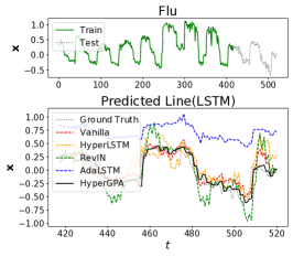
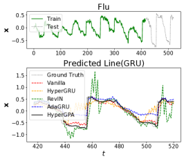
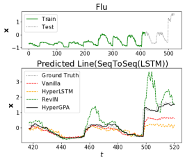
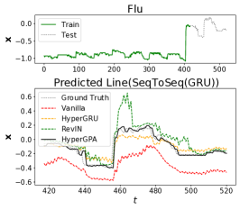
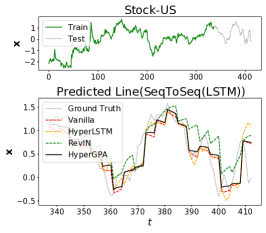
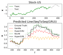
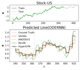
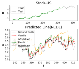
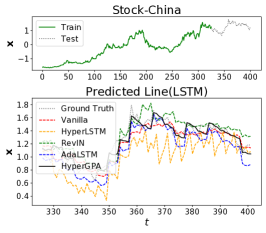
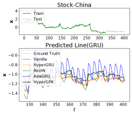
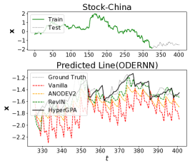
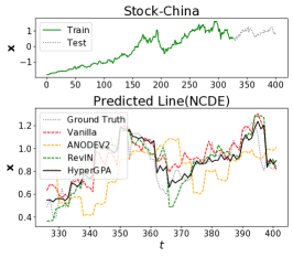
Figure 9. Forecasting visualizations of the baselines and HyperGPA

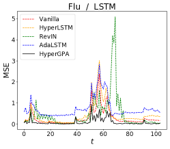
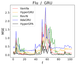
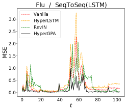
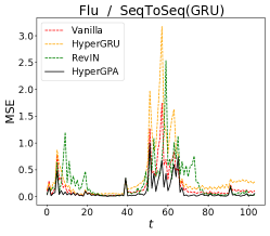
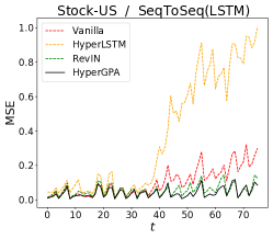
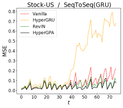
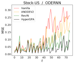
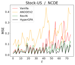
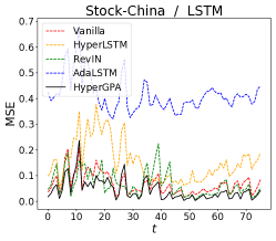
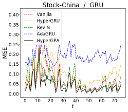
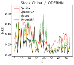
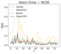
Figure 10. MSE over time

References

- (1)
- REN (2021) 2021. Deep Learning-Based Weather Prediction: A Survey. Big Data Research 23 (2021), 100178. https://doi.org/10.1016/j.bdr.2020.100178
- Ariyo et al. (2014) Adebiyi A. Ariyo, Adewumi O. Adewumi, and Charles K. Ayo. 2014. Stock Price Prediction Using the ARIMA Model. In 2014 UKSim-AMSS 16th International Conference on Computer Modelling and Simulation. 106–112. https://doi.org/10.1109/UKSim.2014.67
- Bai et al. (2020) Lei Bai, Lina Yao, Can Li, Xianzhi Wang, and Can Wang. 2020. Adaptive Graph Convolutional Recurrent Network for Traffic Forecasting. arXiv:2007.02842 [cs.LG]
- Ben-David et al. (2007) Shai Ben-David, John Blitzer, Koby Crammer, and Fernando Pereira. 2007. Analysis of Representations for Domain Adaptation. In Advances in Neural Information Processing Systems, B. Schölkopf, J. Platt, and T. Hoffman (Eds.), Vol. 19. MIT Press.
- Brouwer et al. (2019) Edward De Brouwer, Jaak Simm, Adam Arany, and Yves Moreau. 2019. GRU-ODE-Bayes: Continuous modeling of sporadically-observed time series. In NeurIPS.
- CDC (1946) CDC. 1946. Centers for Disease Control and Prevention. https://www.cdc.gov/.
- Chen et al. (2019) Ricky T. Q. Chen, Yulia Rubanova, Jesse Bettencourt, and David Duvenaud. 2019. Neural Ordinary Differential Equations. arXiv:1806.07366 [cs.LG]
- Cho et al. (2014) Kyunghyun Cho, Bart van Merrienboer, Caglar Gulcehre, Dzmitry Bahdanau, Fethi Bougares, Holger Schwenk, and Yoshua Bengio. 2014. Learning Phrase Representations using RNN Encoder-Decoder for Statistical Machine Translation. arXiv:1406.1078 [cs.CL]
- Du et al. (2021) Yuntao Du, Jindong Wang, Wenjie Feng, Sinno Pan, Tao Qin, Renjun Xu, and Chongjun Wang. 2021. AdaRNN: Adaptive Learning and Forecasting of Time Series. https://doi.org/10.48550/ARXIV.2108.04443
- Ha et al. (2016) David Ha, Andrew Dai, and Quoc V. Le. 2016. HyperNetworks. arXiv:1609.09106 [cs.LG]
- Henning et al. (2018) Christian Andreas Henning, Johannes von Oswald, João Sacramento, Simone Carlo Surace, Jean-Pascal Pfister, and Benjamin F. Grewe. 2018. Approximating the Predictive Distribution via Adversarially-Trained Hypernetworks.
- Hillmer and Tiao (1982) S. C. Hillmer and G. C. Tiao. 1982. An ARIMA-Model-Based Approach to Seasonal Adjustment. J. Amer. Statist. Assoc. 77, 377 (1982), 63–70. https://doi.org/10.1080/01621459.1982.10477767 arXiv:https://www.tandfonline.com/doi/pdf/10.1080/01621459.1982.10477767
- Hochreiter and Schmidhuber (1997) Sepp Hochreiter and Jürgen Schmidhuber. 1997. Long Short-term Memory. Neural computation 9 (12 1997), 1735–80. https://doi.org/10.1162/neco.1997.9.8.1735
- Investing.com (2007) Investing.com. 2007. Stock Datasets. https://www.investing.com/.
- Jeon et al. (2022) Jinsung Jeon, Jeonghak Kim, Haryong Song, Seunghyeon Cho, and Noseong Park. 2022. GT-GAN: General Purpose Time Series Synthesis with Generative Adversarial Networks. https://doi.org/10.48550/ARXIV.2210.02040
- Jhin et al. (2022) Sheo Yon Jhin, Jaehoon Lee, Minju Jo, Seungji Kook, Jinsung Jeon, Jihyeon Hyeong, Jayoung Kim, and Noseong Park. 2022. EXIT: Extrapolation and Interpolation-based Neural Controlled Differential Equations for Time-series Classification and Forecasting. https://doi.org/10.48550/ARXIV.2204.08771
- Kidger et al. (2020) Patrick Kidger, James Morrill, James Foster, and Terry Lyons. 2020. Neural Controlled Differential Equations for Irregular Time Series. arXiv:2005.08926 [cs.LG]
- Kim et al. (2022) Taesung Kim, Jinhee Kim Kim, Yunwon Tae, Cheonbok Park, Jang-Ho Choi Choi, and Jaegul Choo. 2022. Reversible Instance Normalization for Accurate Time-Series Forecasting against Distribution Shift. In Submitted to The Tenth International Conference on Learning Representations.
- Kipf and Welling (2017) Thomas N. Kipf and Max Welling. 2017. Semi-Supervised Classification with Graph Convolutional Networks. arXiv:1609.02907 [cs.LG]
- Krueger et al. (2017) David Krueger, Chin-Wei Huang, Riashat Islam, Ryan Turner, Alexandre Lacoste, and Aaron Courville. 2017. Bayesian Hypernetworks. https://doi.org/10.48550/ARXIV.1710.04759
- Kuznetsov et al. (2015) Kuznetsov, Vitaly, Mohri, and Mehryar. 2015. Learning Theory and Algorithms for Forecasting Non-stationary Time Series. In Advances in Neural Information Processing Systems, C. Cortes, N. Lawrence, D. Lee, M. Sugiyama, and R. Garnett (Eds.), Vol. 28. Curran Associates, Inc.
- Kuznetsov and Mohri (2014) Vitaly Kuznetsov and Mehryar Mohri. 2014. Generalization Bounds for Time Series Prediction with Non-stationary Processes. In Algorithmic Learning Theory, Peter Auer, Alexander Clark, Thomas Zeugmann, and Sandra Zilles (Eds.). Springer International Publishing, Cham, 260–274.
- Li et al. (2018) Haoliang Li, Sinno Jialin Pan, Shiqi Wang, and Alex C. Kot. 2018. Domain Generalization with Adversarial Feature Learning. In 2018 IEEE/CVF Conference on Computer Vision and Pattern Recognition. 5400–5409. https://doi.org/10.1109/CVPR.2018.00566
- Li et al. (2021) Zijian Li, Ruichu Cai, Tom Z. J. Fu, and Kun Zhang. 2021. Transferable Time-Series Forecasting under Causal Conditional Shift. CoRR abs/2111.03422 (2021). arXiv:2111.03422
- Littwin and Wolf (2019) Gidi Littwin and Lior Wolf. 2019. Deep Meta Functionals for Shape Representation. https://doi.org/10.48550/ARXIV.1908.06277
- Muandet et al. (2013) Krikamol Muandet, David Balduzzi, and Bernhard Schölkopf. 2013. Domain Generalization via Invariant Feature Representation. https://doi.org/10.48550/ARXIV.1301.2115
- Nachmani and Wolf (2019) Eliya Nachmani and Lior Wolf. 2019. Hyper-Graph-Network Decoders for Block Codes. https://doi.org/10.48550/ARXIV.1909.09036
- Oh et al. (2019) Jeeheh Oh, Jiaxuan Wang, Shengpu Tang, Michael W. Sjoding, and Jenna Wiens. 2019. Relaxed Parameter Sharing: Effectively Modeling Time-Varying Relationships in Clinical Time-Series. Proceedings of Machine Learning Research 106 (2019).
- Oswald et al. (2020) Johannes Oswald, Christian Henning, João Sacramento, and Benjamin F. Grewe. 2020. Continual learning with hypernetworks. arXiv:1906.00695 [cs.LG]
- Pan et al. (2019) Zheyi Pan, Yuxuan Liang, Weifeng Wang, Yong Yu, Yu Zheng, and Junbo Zhang. 2019. Urban Traffic Prediction from Spatio-Temporal Data Using Deep Meta Learning. In Proceedings of the 25th ACM SIGKDD International Conference on Knowledge Discovery & Data Mining (Anchorage, AK, USA) (KDD ’19). Association for Computing Machinery, New York, NY, USA, 1720–1730. https://doi.org/10.1145/3292500.3330884
- Pawlowski et al. (2018) Nick Pawlowski, Andrew Brock, Matthew C. H. Lee, Martin Rajchl, and Ben Glocker. 2018. Implicit Weight Uncertainty in Neural Networks. arXiv:1711.01297 [stat.ML]
- Peng et al. (2021) Jiaqi Peng, Jinxia Guo, Qinli Yang, Jianyun Lu, and Junmming Shao. 2021. A general framework for mining concept-drifting data streams with evolvable features. In 2021 IEEE International Conference on Data Mining (ICDM). 1276–1281. https://doi.org/10.1109/ICDM51629.2021.00157
- Rubanova et al. (2019) Yulia Rubanova, Ricky T. Q. Chen, and David Duvenaud. 2019. Latent ODEs for Irregularly-Sampled Time Series. arXiv:1907.03907 [cs.LG]
- Shamsian et al. (2021) Aviv Shamsian, Aviv Navon, Ethan Fetaya, and Gal Chechik. 2021. Personalized Federated Learning using Hypernetworks. In Proceedings of the 38th International Conference on Machine Learning (Proceedings of Machine Learning Research, Vol. 139), Marina Meila and Tong Zhang (Eds.). PMLR, 9489–9502.
- Sutskever et al. (2014) Ilya Sutskever, Oriol Vinyals, and Quoc V Le. 2014. Sequence to sequence learning with neural networks. In NeurIPS. 3104–3112.
- Tzeng et al. (2017) Eric Tzeng, Judy Hoffman, Kate Saenko, and Trevor Darrell. 2017. Adversarial Discriminative Domain Adaptation. https://doi.org/10.48550/ARXIV.1702.05464
- USHCN (1987) USHCN. 1987. US Historical Climatology Network. https://www.ncei.noaa.gov.
- Vaswani et al. (2017) Ashish Vaswani, Noam Shazeer, Niki Parmar, Jakob Uszkoreit, Llion Jones, Aidan N. Gomez, Lukasz Kaiser, and Illia Polosukhin. 2017. Attention Is All You Need. https://doi.org/10.48550/ARXIV.1706.03762
- Veličković et al. (2018) Petar Veličković, Guillem Cucurull, Arantxa Casanova, Adriana Romero, Pietro Liò, and Yoshua Bengio. 2018. Graph Attention Networks. arXiv:1710.10903 [stat.ML]
- Vijh et al. (2020) Mehar Vijh, Deeksha Chandola, Vinay Anand Tikkiwal, and Arun Kumar. 2020. Stock Closing Price Prediction using Machine Learning Techniques. Procedia Computer Science (2020). https://doi.org/10.1016/j.procs.2020.03.326
- Wang et al. (2021a) Jindong Wang, Cuiling Lan, Chang Liu, Yidong Ouyang, Tao Qin, Wang Lu, Yiqiang Chen, Wenjun Zeng, and Philip S. Yu. 2021a. Generalizing to Unseen Domains: A Survey on Domain Generalization. https://doi.org/10.48550/ARXIV.2103.03097
- Wang et al. (2021b) Rui Wang, Danielle Maddix, Christos Faloutsos, Yuyang Wang, and Rose Yu. 2021b. Bridging Physics-based and Data-driven modeling for Learning Dynamical Systems. In Proceedings of the 3rd Conference on Learning for Dynamics and Control (Proceedings of Machine Learning Research), Ali Jadbabaie, John Lygeros, George J. Pappas, Pablo A. Parrilo, Benjamin Recht, Claire J. Tomlin, and Melanie N. Zeilinger (Eds.). PMLR.
- Wu et al. (2020) Neo Wu, Bradley Green, Xue Ben, and Shawn O’Banion. 2020. Deep Transformer Models for Time Series Forecasting: The Influenza Prevalence Case. arXiv:2001.08317 [cs.LG]
- Zhang et al. (2018) Chris Zhang, Mengye Ren, and Raquel Urtasun. 2018. Graph HyperNetworks for Neural Architecture Search. https://doi.org/10.48550/ARXIV.1810.05749
- Zhang et al. (2013) Kun Zhang, Bernhard Schölkopf, Krikamol Muandet, and Zhikun Wang. 2013. Domain Adaptation under Target and Conditional Shift. In ICML.
- Zhang et al. (2019) Tianjun Zhang, Zhewei Yao, Amir Gholami, Kurt Keutzer, Joseph Gonzalez, George Biros, and Michael Mahoney. 2019. ANODEV2: A Coupled Neural ODE Evolution Framework. arXiv:1906.04596 [cs.LG]
- Zhu et al. (2021) Yongchun Zhu, Fuzhen Zhuang, Jindong Wang, Guolin Ke, Jingwu Chen, Jiang Bian, Hui Xiong, and Qing He. 2021. Deep Subdomain Adaptation Network for Image Classification. IEEE Transactions on Neural Networks and Learning Systems 32, 4 (2021), 1713–1722. https://doi.org/10.1109/TNNLS.2020.2988928