A neuron-wise subspace correction method for
the finite neuron method

Abstract

In this paper, we propose a novel algorithm called Neuron-wise Parallel Subspace Correction Method (NPSC) for the finite neuron method that approximates numerical solutions of partial differential equations (PDEs) using neural network functions. Despite extremely extensive research activities in applying neural networks for numerical PDEs, there is still a serious lack of effective training algorithms that can achieve adequate accuracy, even for one-dimensional problems. Based on recent results on the spectral properties of linear layers and landscape analysis for single neuron problems, we develop a special type of subspace correction method that optimizes the linear layer and each neuron in the nonlinear layer separately. An optimal preconditioner that resolves the ill-conditioning of the linear layer is presented for one-dimensional problems, so that the linear layer is trained in a uniform number of iterations with respect to the number of neurons. In each single neuron problem, a good local minimum that avoids flat energy regions is found by a superlinearly convergent algorithm. Numerical experiments on function approximation problems and PDEs demonstrate better performance of the proposed method than other gradient-based methods.

65D15, 65N22, 65N30, 65N55, 68T07

1 Introduction

Neural networks, thanks to the universal approximation property [8, 24], are promising tools for numerical solutions of partial differential equations (PDEs). Moreover, it was shown in [28] that the approximation properties of neural networks have higher asymptotic approximation rates than that of traditional numerical methods such as the finite element method. Such powerful approximation properties, however, can hardly be observed in numerical experiments in simple tasks of function approximation despite extensive research on numerical solutions of PDEs in recent years, e.g., physics-informed neural networks [25], the deep Ritz method [10], and the finite neuron method [38]. Even in one dimension, using gradient-based methods to training a shallow neural network does not produce accurate solutions with a substantial number of iterations. This poor convergence behavior was analyzed rigorously in [14] and is due to the ill-conditioning of problem. Therefore, applying neural networks to solutions of PDEs must require novel training algorithms, different from the conventional ones for regression, image classification, and pattern recognition tasks. In this viewpoint, there are many works on designing and analyzing training algorithms for neural networks to try to speed up the convergence or narrow the gap between the theoretical optimum and training results. For instance, a hybrid least squares/gradient descent method was proposed in [9] from an adaptive basis perspective. The active neuron least squares method in [2] was designed to avoid plateau phenomena that slow down the gradient dynamics of training ReLU shallow neural networks [1, 21]. In addition, as a completely different approach, the orthogonal greedy algorithm was shown to achieve an optimal convergence rate [29, 30].

The aim of this paper is to develop a novel training algorithm using several recent theoretical results on training of neural networks. A surprising recent result on training of neural networks shows that optimizing the linear layer parameters in a neural network is one bottleneck that leads to a large number of iterations of a gradient-based method. More precisely, it was proven in [14] that optimizing the linear layer parameters in a ReLU shallow neural network requires solving a very ill-conditioned linear problem in general. This work motivates us to separately design efficient solvers for the outer linear layer and the inner nonlinear layer, respectively, and train them alternately.

Meanwhile, some recent works suggest that learning a single neuron may be a more hopeful task than learning a nonlinear layer with multiple neurons. In [31, 33, 41], convergence analyses of gradient methods for the single neuron problem with ReLU activation were presented under various assumptions on input distributions. In [35], the case of a single ReLU neuron with bias was analyzed. All of these results show that the global convergence of gradient methods for the single ReLU neuron problem can be attained under certain conditions.

Inspired by the above results, we consider training of the finite neuron method in one dimension as an example, and use the well-known framework of subspace correction [37] to combine insights from the spectral properties of linear layers [14] and landscape analysis for single neuron problems [35]. Subspace correction methods provide a unified framework to design and analyze many modern iterative numerical methods such as block coordinate descent, multigrid, and domain decomposition methods. Mathematical theory of subspace correction methods for convex optimization problems is established in [22, 32], and successful applications of it to various nonlinear optimization problems in engineering fields can be found in, e.g., [3, 18]. In particular, there have been successful applications of block coordinate descent methods [36] for training of neural networks [42, 43]. Therefore, we expect that the idea of the subspace correction method is also suitable for training of neural networks for the finite neuron method.

We propose a new training algorithm called Neuron-wise Parallel Subspace Correction Method (NPSC), which is a special type of subspace correction method for the finite neuron method [38]. The proposed method utilizes a space decomposition for the linear layer and each individual neuron. In the first step of each epoch of the NPSC, the linear layer is fully trained by solving a linear system using an iterative solver. We prove, both theoretically and numerically, that we can design an optimal preconditioner for the linear layer for one-dimensional problems, based on the relation between ReLU neural networks and linear finite elements investigated in [11, 14]. In the second step, we train each single neuron in parallel, taking advantages of better convergence properties of learning a single neuron and a superlinearly convergent algorithm [19]. Finally, an update for the parameters in the nonlinear layer is computed by assembling the corrections obtained in the local problems for each neuron. Due to the intrinsic parallel structure, NPSC is suitable for parallel computation on distributed memory computers. We present applications of NPSC to various function approximation problems and PDEs, and numerically verify that it outperforms conventional training algorithms.

The rest of this paper is organized as follows. In Section 2, we summarize key features of the finite neuron method with ReLU shallow neural networks, and state a model problem. An optimal preconditioner for the linear layer in one dimension is presented in Section 3. NPSC, our proposed algorithm, is presented in Section 4. Applications of NPSC to various function approximation problems and PDEs are presented in Section 5 to demonstrate the effectiveness of NPSC. We conclude the paper with remarks in Section 6.

2 Finite neuron method

In this section, we introduce the finite neuron method [38] with ReLU shallow neural networks to approximate solutions of PDEs. We also discuss the ill-conditioning of ReLU shallow neural network [14], which reveals the difficulty of training ReLU shallow neural network using gradient-based methods.

2.1 Model problem

We consider the following model problem:

(1) $$\min_{u\in V}\left\{\frac{1}{2}a(u,u)-\int_{\Omega}fu\,dx\right\},$$

where $\Omega\subset\mathbb{R}^{d}$ is a bounded domain, $f\in L^{2}(\Omega)$, $a(\cdot,\cdot)$ is a continuous, coercive, and symmetric bilinear form defined on a Hilbert space $V\subset L^{2}(\Omega)$. Various elliptic boundary value problems can be formulated as optimization problems of the form (1) [38].

A ReLU shallow neural network with $n$ neurons is given by

(2) $$u(x;\theta)=\sum_{i=1}^{n}a_{i}\sigma(\omega_{i}\cdot x+b_{i}),\quad\theta=\left\{a,\omega,b\right\}=\left\{(a_{i})_{i=1}^{n},(\omega_{i})_{i=1}^{n},(b_{i})_{i=1}^{n}\right\},$$

where $x\in\mathbb{R}^{d}$ is an input, $\theta$ is the collection of parameters consisting of $a_{i}\in\mathbb{R}$, $\omega_{i}\in\mathbb{R}^{d}$, and $b_{i}\in\mathbb{R}$ for $1\leq i\leq n$, and $\sigma\colon\mathbb{R}\rightarrow\mathbb{R}$ is the ReLU activation function defined by $\sigma(x)=\max\{0,x\}$. The neural network (2) possesses a total of $(d+2)n$ parameters.

The collection of all neural network functions of the form (2) is denoted by $\Sigma_{n}$, i.e.,

$$\Sigma_{n}=\left\{v(x)=\sum_{i=1}^{n}a_{i}\sigma(\omega_{i}\cdot x+b_{i}):a_{i}\in\mathbb{R},\hskip 2.84544pt\omega_{i}\in\mathbb{R}^{d},\hskip 2.84544ptb_{i}\in\mathbb{R}\right\}.$$

The space $\cup_{n\in\mathbb{N}}\Sigma_{n}$ enjoys the universal approximation property [8, 24], namely, any function with sufficient regularity can be uniformly approximated by functions in $\cup_{n\in\mathbb{N}}\Sigma_{n}$. Recent results on such approximation properties can be found in [28, 30].

In the finite neuron method, we consider the Galerkin approximation of (1) on the space $\Sigma_{n}$:

$$\min_{u\in\Sigma_{n}}\left\{\frac{1}{2}a(u,u)-\int_{\Omega}fu\,dx\right\},$$

which is equivalent to

(3) $$\min_{\theta\in\Theta}\left\{E(\theta):=\frac{1}{2}a\left(u(x;\theta),u(x;\theta)\right)-\int_{\Omega}f(x)u(x;\theta)\,dx\right\},$$

where $\Theta=\mathbb{R}^{(d+2)n}$ is the parameter space. That is, in (3), we find a good approximation of the solution of the continuous problem (1) in terms of the neural network (2).

2.2 Ill-conditioning of the linear layer

From the structure of the neural network (2), we say that the parameter $a$ belongs to the linear layer and $\omega$ and $b$ belong to the nonlinear layer. In this subsection, we explain that even optimizing parameters in the linear layer becomes a bottleneck if we use simple gradient-based methods. A large number of iterations is needed to achieve satisfatory accuracy due to the ill-conditioning of the linear layer.

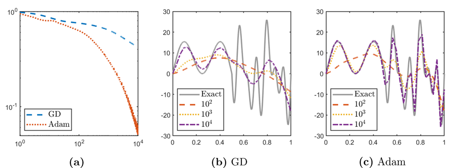
Figure 1: Numerical results for the function approximation problem (5). (a) Decay of the relative energy error $\frac{E_{M}(a^{(k)})-E_{M}(M^{-1}\beta)}{|E_{M}(M^{-1}\beta)|}$ in the gradient descent method (GD) and Adam, where $k$ denotes the number of iterations. (b, c) Exact solution and its approximations generated by various numbers of iterations of GD and Adam ($n=2^{5}$).

To illustrate the ill-conditioning, we consider $\Omega=(0,1)\subset\mathbb{R}$ and the following bilinear form

(4) $$a(u,v)=\int_{\Omega}uv\,dx,\quad u,v\in V,\quad V=L^{2}(\Omega)$$

in (3). We obtain the $L^{2}$-function approximation problem, which is the most elementary instance of (3). We fix the parameters $\omega$ and $b$ in (3) as follows:

$$\omega_{i}=1,\quad b_{i}=-\frac{i-1}{n},\quad 1\leq i\leq n.$$

Then (3) is written as

(5) $$\min_{a\in\mathbb{R}^{n}}\left\{E_{M}(a):=\frac{1}{2}a^{\mathrm{T}}Ma-\beta^{\mathrm{T}}a\right\},$$

where $M\in\mathbb{R}^{n\times n}$ and $\beta\in\mathbb{R}^{n}$ are given by

$$\begin{aligned} &M_{ij}=\int_{\Omega}\sigma\left(x-\frac{j-1}{n}\right)\sigma\left(x-\frac{i-1}{n}\right)\,dx,\\ &\beta_{i}=\int_{\Omega}f(x)\sigma\left(x-\frac{i-1}{n}\right)\,dx,\end{aligned}\quad 1\leq i,j\leq n.$$

When we solve the minimization problem (5) by a gradient-based method such as the gradient descent method or Adam [15], the convergence rate depends on the condition number $\kappa(M)$ of $M$. It was recently proved in [14, Theorem 1] that $M$ is very ill-conditioned. This result is stated in the following proposition.

Proposition 2.1.

In (5), the condition number $\kappa(M)$ of the matrix $M$ satisfies

$$\kappa(M)=O(n^{4}).$$

The condition number $\kappa(M)$ becomes exceedingly large when $n$ increases. The convergence of simple gradient-based methods thus becomes extremely slow. We now demonstrate the poor convergence of the gradient descent method and Adam for solving (5) with $f$ given by

(6) $$f(x)=\begin{cases}10\left(\sin 2\pi x+\sin 6\pi x\right),&\quad\textrm{ if }0<x<\frac{1}{2},\\ 10\left(\sin 8\pi x+\sin 18\pi x+\sin 26\pi x\right),&\quad\textrm{ if }\frac{1}{2}\leq x<1.\end{cases}$$

In both methods, the learning rate $\tau$ is chosen as $\tau=2/(\lambda_{\min}(M)+\lambda_{\max}(M))$, which is optimal in the sense of [34, Lemma C.5]; $\lambda_{\min}$ and $\lambda_{\max}$ stand for the minimum and maximum eigenvalues, respectively. We use the zero initial guess. One can observe in Fig. 1(a) that the convergence rates of both methods are fairly slow even when $n$ is not large; the relative energy error $\frac{E_{M}(a^{(k)})-E_{M}(M^{-1}\beta)}{|E_{M}(M^{-1}\beta)|}$ does not reach $10^{-2}$ with $10^{4}$ iterations. Moreover, as shown in Fig. 1(b, c), both methods give poor numerical approximations to $f$ despite large numbers of iterations.

3 Optimal preconditioner for the linear layer in one dimension

In this section, we propose an optimal preconditioner for the linear layer in one dimension. Using the proposed preconditioner, the linear layer can be fully trained within a uniform number of iterations with respect to the number of neurons $n$.

For simplicity, we set $\Omega=(0,1)\subset\mathbb{R}$ in (3). Fixing the parameters $\omega$ and $b$ in the nonlinear layer, (3) reduces to the following minimization problem with respect to $a$:

(7) $$\min_{a\in\mathbb{R}^{n}}\left\{\frac{1}{2}a^{\mathrm{T}}Ka-\beta^{\mathrm{T}}a\right\},$$

where $K\in\mathbb{R}^{n\times n}$ and $\beta\in\mathbb{R}^{n}$ are given by

(8) $$\begin{aligned} &K_{ij}=a\left(\sigma(\omega_{j}x+b_{j}),\sigma(\omega_{i}x+b_{i})\right),\\ &\beta_{i}=\int_{\Omega}f(x)\sigma(\omega_{i}x+b_{i})\,dx,\end{aligned}\quad 1\leq i,j\leq n.$$

Let

$$x_{i}=-\frac{b_{i}}{\omega_{i}},\quad 1\leq i\leq n,$$

be the nodal point determined by the ReLU function $\psi_{i}(x)=\sigma(\omega_{i}x+b_{i})$. We denote the number of the nodal points inside $\Omega$ by $n_{\Omega}$. Without loss of generality, we assume the following:

(9a) $$\psi_{i}\not\equiv 0\text{ on }\Omega,\quad 1\leq i\leq n,$$

(9b) $$n_{\Omega}\geq n-2,$$

(9c) $$x_{1},\dots,x_{n_{\Omega}}\in\Omega\hskip 2.84544pt\text{ and }\hskip 2.84544ptx_{1}<\dots<x_{n_{\Omega}},$$

(9d) $$x_{n_{\Omega+1}},\dots,x_{n}\in\mathbb{R}\setminus\Omega\hskip 2.84544pt\text{ and }\hskip 2.84544ptx_{n_{\Omega+1}}<\dots<x_{n}.$$

The assumption (9a) requires that no $\psi_{i}$ vanishes on $\Omega$ because otherwise they do not contribute to the minimization problem (7). The assumption (9b) requires at most two neurons with nodal points outside $\Omega$. This is because the corresponding ReLU functions become linearly dependent on $\Omega$ if there are more than two neurons with nodal points outside $\Omega$. Finally, the assumptions (9c) and (9d) can be satisfied under an appropriate reordering.

Under (9), it is proved in [11, Theorem 2.1] that $\{\psi_{i}\}_{i=1}^{n}$ are linearly independent on $\Omega$. It is easy to see $K$ is symmetric and positive definite (SPD). Let $\mathcal{A}\colon V\rightarrow V$ be a bijective linear operator such that

(10) $$a(u,v)=\int_{\Omega}(\mathcal{A}u)v\,dx,\quad u,v\in V.$$

Writing $\Psi=[\psi_{1},\dots,\psi_{n}]^{\mathrm{T}}$, we have

$$K=\int_{\Omega}(\mathcal{A}\Psi(x))\Psi(x)^{\mathrm{T}}\,dx,$$

where $\mathcal{A}$ is applied entrywise.

Before we present the optimal preconditioner, we state the following lemma that is used in the construction of the proposed preconditioner.

Lemma 3.1.

For two positive integers $m\geq n$, let $A$, $B\in\mathbb{R}^{m\times m}$ be two SPD matrices and let $R\in\mathbb{R}^{n\times m}$ be a surjective matrix. Then $RB^{-1}R^{\mathrm{T}}$ is SPD and

$$\kappa\left(\left(RB^{-1}R^{\mathrm{T}}\right)^{-1}RAR^{\mathrm{T}}\right)\leq\kappa(BA).$$

Proof 3.2.

It is easy to see that $B^{-1}$ is SPD and $R^{\mathrm{T}}$ is injective. Then we have

$$\langle RB^{-1}R^{\mathrm{T}}\alpha,\alpha\rangle=\langle B^{-1}R^{\mathrm{T}}\alpha,R^{\mathrm{T}}\alpha\rangle>0,\quad\forall\alpha\neq\mathbf{0}.$$

Hence, $RB^{-1}R^{T}$ is also SPD.

One can establish a lower bound for the minimum eigenvalue of the matrix $(RB^{-1}R^{\mathrm{T}})^{-1}RAR^{\mathrm{T}}$ as follows:

(11) $$\lambda_{\min}\left(\left(RB^{-1}R^{\mathrm{T}}\right)^{-1}RAR^{\mathrm{T}}\right)=\min_{\alpha\neq\mathbf{0}}\frac{\alpha^{\mathrm{T}}RAR^{\mathrm{T}}\alpha}{\alpha^{\mathrm{T}}RB^{-1}R^{\mathrm{T}}\alpha}\\ =\min_{\begin{subarray}{c}\bar{\alpha}\in\operatorname{ran}R^{\mathrm{T}},\\ \bar{\alpha}\neq\mathbf{0}\end{subarray}}\frac{\bar{\alpha}^{\mathrm{T}}A\bar{\alpha}}{\bar{\alpha}^{\mathrm{T}}B^{-1}\bar{\alpha}}\geq\min_{\bar{\alpha}\neq\mathbf{0}}\frac{\bar{\alpha}^{\mathrm{T}}A\bar{\alpha}}{\bar{\alpha}^{\mathrm{T}}B^{-1}\bar{\alpha}}=\lambda_{\min}(BA).$$

In the same manner, we have

(12) $$\lambda_{\max}\left(\left(RB^{-1}R^{\mathrm{T}}\right)^{-1}RAR^{\mathrm{T}}\right)\leq\lambda_{\max}(BA).$$

Combining (11) and (12) yields the desired result.

Now we are ready to construct our proposed preconditioner, which resolves the issue of ill-conditioning explained in Section 2.

We define

$$\psi_{\mathrm{L}}(x)=x,\quad\psi_{\mathrm{R}}(x)=1-x,$$

and write $\overline{\Psi}=[\psi_{1},\dots,\psi_{n_{\Omega}},\psi_{\mathrm{L}},\psi_{\mathrm{R}}]^{\mathrm{T}}$. Since each $\psi_{i}$, $n_{\Omega}+1\leq i\leq n$, is linear on $\Omega$, we have

$$\psi_{i}=\psi_{i}(1)\psi_{\mathrm{L}}+\psi_{i}(0)\psi_{\mathrm{R}}\hskip 2.84544pt\text{ on }\hskip 2.84544pt\Omega.$$

Hence, we readily get $\Psi=R\overline{\Psi}$ on $\Omega$, where

(13) $$R=\begin{bmatrix}I_{n_{\Omega}}&\mathbf{0}\\ \mathbf{0}&\widetilde{R}\end{bmatrix}\in\mathbb{R}^{n\times(n_{\Omega}+2)},\quad\widetilde{R}=\begin{bmatrix}\psi_{n_{\Omega}+1}(1)&\psi_{n_{\Omega}+1}(0)\\ \vdots&\vdots\\ \psi_{n}(1)&\psi_{n}(0)\end{bmatrix}\in\mathbb{R}^{(n-n_{\Omega})\times 2}.$$

In (13), $I_{n_{\Omega}}$ denotes the $\mathbb{R}^{n_{\Omega}\times n_{\Omega}}$ identity matrix.

We define

(14) $$\overline{K}=\int_{\Omega}(\mathcal{A}\overline{\Psi}(x))\overline{\Psi}(x)^{\mathrm{T}}\,dx.$$

It is easy to see $M=R\overline{K}R^{\mathrm{T}}$. Invoking [11, Theorem 2.1] implies that the entries of $\overline{\Psi}$ are linearly independent, so that they form a basis for the space $V_{n_{\Omega}+2}$ of continuous and piecewise linear functions on the grid $0<x_{1}<\dots<x_{n_{\Omega}}<1$.

If we set $\overline{\Psi}^{+}=[\psi_{1}^{+},\dots,\psi_{n_{\Omega}}^{+},\psi_{\mathrm{L}},\psi_{\mathrm{R}}]^{\mathrm{T}}$, where

$$\psi_{i}^{+}(x)=\sigma(x-x_{i}),\quad 1\leq i\leq n_{\Omega},$$

then by direct calculation we get

(15) $$\psi_{i}=\begin{cases}\omega_{i}\psi_{i}^{+},&\quad\text{ if }\omega_{i}\geq 0,\\ \omega_{i}(1-x_{i})\psi_{\mathrm{L}}-\omega_{i}\psi_{i}^{+}-\omega_{i}x_{i}\psi_{\mathrm{R}},&\quad\text{ otherwise.}\end{cases}$$

Using (15), it is straightforward to construct a matrix $B_{1}\in\mathbb{R}^{(n_{\Omega}+2)\times(n_{\Omega}+2)}$ satisfying

(16) $$\overline{\Psi}=B_{1}\overline{\Psi}^{+}.$$

The matrix $B_{1}$ is nonsingular since both the entries of $\overline{\Psi}$ and those of $\overline{\Psi}^{+}$ form bases for the space $V_{n_{\Omega+2}}$ [11].

Meanwhile, $V_{n_{\Omega}+2}$ admits the standard hat basis $\{\phi_{1},\dots,\phi_{n_{\Omega}},\phi_{\mathrm{L}},\phi_{\mathrm{R}}\}$, which is given by

$$\phi_{i}(x)=\begin{cases}\dfrac{x-x_{i-1}}{x_{i}-x_{i-1}},&\quad\text{ if }x\in(x_{i-1},x_{i}],\\ \dfrac{x-x_{i+1}}{x_{i}-x_{i+1}},&\quad\text{ if }x\in[x_{i},x_{i+1}),\\ 0,&\quad\text{ otherwise,}\end{cases}\quad 1\leq i\leq n_{\Omega},$$

$$\phi_{\mathrm{L}}(x)=\begin{cases}-\dfrac{x-x_{1}}{x_{1}},&\quad\text{ if }x\in(0,x_{1}],\\ 0,&\quad\text{ otherwise,}\end{cases}\quad\phi_{\mathrm{R}}(x)=\begin{cases}\dfrac{x-x_{n_{\Omega}}}{1-x_{n_{\Omega}}},&\quad\text{ if }x\in[x_{n_{\Omega}},1),\\ 0,&\quad\text{ otherwise,}\end{cases}$$

with abuse of notation $x_{-1}=0$ and $x_{n_{\Omega}+1}=1$. Similar to (14), we write $\overline{\Phi}=[\phi_{1},\dots,\phi_{n_{\Omega}},\phi_{\mathrm{L}},\phi_{\mathrm{R}}]^{\mathrm{T}}$ and set

$$\overline{K}_{\phi}=\int_{\Omega}(\mathcal{A}\overline{\Phi}(x))\overline{\Phi}(x)^{\mathrm{T}}\,dx.$$

One can verify the following relation between the entries of $\overline{\Phi}$ and those of $\overline{\Psi}^{+}$ by direct calculation:

(17) $$\begin{split}\phi_{1}&=\frac{1}{x_{1}}\psi_{\mathrm{L}}-\frac{x_{2}}{(x_{2}-x_{1})x_{1}}\psi_{1}^{+}+\frac{1}{x_{2}-x_{1}}\psi_{2}^{+},\\ \phi_{i}&=\frac{1}{x_{i}-x_{i-1}}\psi_{i-1}^{+}-\frac{x_{i+1}-x_{i-1}}{(x_{i+1}-x_{i})(x_{i}-x_{i-1})}\psi_{i}^{+}+\frac{1}{x_{i+1}-x_{i}}\psi_{i+1}^{+},\hskip 2.84544pt2\leq i\leq n_{\Omega}-1,\\ \phi_{n_{\Omega}}&=\frac{1}{x_{n_{\Omega}}-x_{n_{\Omega}-1}}\psi_{n_{\Omega}-1}^{+}-\frac{1-x_{n_{\Omega}-1}}{(1-x_{n_{\Omega}})(x_{n_{\Omega}}-x_{n_{\Omega}-1})}\psi_{n_{\Omega}}^{+},\\ \phi_{\mathrm{L}}&=-\frac{1-x_{1}}{x_{1}}\psi_{\mathrm{L}}+\frac{1}{x_{1}}\psi_{1}^{+}+\psi_{\mathrm{R}},\\ \phi_{\mathrm{R}}&=\frac{1}{1-x_{n}}\psi_{n_{\Omega}}^{+}.\end{split}$$

Hence, we can construct a matrix $B_{2}\in\mathbb{R}^{(n_{\Omega}+2)\times(n_{\Omega}+2)}$ such that

(18) $$\overline{\Phi}=B_{2}\overline{\Psi}^{+}$$

explicitly using (17). Combining (16) and (18) yields

(19) $$\overline{\Phi}=B\overline{\Psi},$$

where $B=B_{2}B_{1}^{-1}$. Equation 19 implies that two matrices $\overline{K}$ and $\overline{K}_{\phi}$ are related as follows:

(20) $$\overline{K}=\int_{\Omega}(\mathcal{A}\overline{\Psi}(x))\overline{\Psi}(x)^{\mathrm{T}}\,dx=\int_{\Omega}B^{-1}(\mathcal{A}\overline{\Phi}(x))\overline{\Phi}(x)^{\mathrm{T}}B^{-\mathrm{T}}\,dx=B^{-1}\overline{K}_{\phi}B^{-\mathrm{T}}.$$

Since $M=R\overline{K}R^{\mathrm{T}}$, invoking Lemma 3.1, setting $\overline{P}=B^{\mathrm{T}}\overline{K}_{\phi}^{-1}B$ and

(21) $$P=\left(R\overline{P}^{-1}R^{\mathrm{T}}\right)^{-1}$$

completes the construction of the proposed preconditioner, where $R$ was defined in (13). We summarize our main result described above in the following theorem.

Theorem 3.3.

Let $\Omega=(0,1)\subset\mathbb{R}$ and let $K\in\mathbb{R}^{n\times n}$ be the matrix defined in (8). Assume that (9) holds. Then the preconditioner $P\in\mathbb{R}^{n\times n}$ given in (21) satisfies

$$\kappa(PK)=O(1),$$

i.e., $\kappa(PK)$ has an upper bound independent of $n$, $\omega$, and $b$.

The proposed preconditioner $P$ can be implemented very efficiently, requiring only $O(n)$ elementary arithmetic operations. Details of the implementation of the proposed preconditioner are discussed in Appendix A.

Remark 3.4.

In the case of the $L^{2}$-function approximation problem (4), we can construct an alternative preconditioner $P_{\operatorname{diag}}$ whose computational cost is a bit cheaper than $P$. Let $\overline{P}_{\operatorname{diag}}=B^{\mathrm{T}}\operatorname{diag}(\overline{K}_{\phi})^{-1}B$. It follows from (20) that

$$\overline{P}_{\operatorname{diag}}\overline{K}=B^{\mathrm{T}}\operatorname{diag}(\overline{K}_{\phi})^{-1}B\overline{K}=B^{\mathrm{T}}\operatorname{diag}(\overline{K}_{\phi})^{-1}\overline{K}_{\phi}B^{-\mathrm{T}}.$$

In (4), $\overline{K}_{\phi}$ is a mass matrix for the linear finite element method defined on the grid $0<x_{1}<\dots<x_{n_{\Omega}}<1$, so that it satisfies $\kappa(\operatorname{diag}(\overline{K}_{\phi})^{-1}\overline{K}_{\phi})=O(1)$. Then we have

$$\kappa(\overline{P}_{\operatorname{diag}}\,\overline{K})=\kappa(B^{\mathrm{T}}\operatorname{diag}(\overline{K}_{\phi})^{-1}\overline{K}_{\phi}B^{-\mathrm{T}})=\kappa(\operatorname{diag}(\overline{K}_{\phi})^{-1}\overline{K}_{\phi})=O(1).$$

Therefore, $P_{\operatorname{diag}}=(R\overline{P}_{\operatorname{diag}}^{-1}R^{\mathrm{T}})^{-1}$ satisfies $\kappa(P_{\operatorname{diag}}K)=O(1)$ by Lemma 3.1. It is evident that the computational cost of $\operatorname{diag}(\overline{K}_{\phi})^{-1}$ is cheaper than that of $\overline{K}_{\phi}^{-1}$.

4 Neuron-wise Parallel Subspace Correction Method (NPSC)

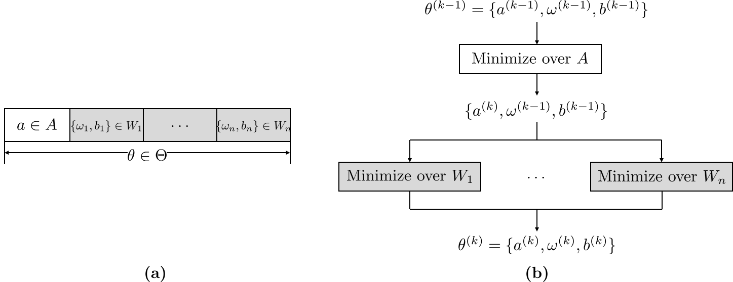
Figure 2: (a) Space decomposition of the solution space $\Theta$ of (3) into subspaces $A$ and $\{W_{i}\}_{i=1}^{n}$. (b) Subspace correction procedure of NPSC.

In this section, we introduce NPSC, a subspace correction method [37] that deals with the linear layer and each neuron in the nonlinear layer separately for solving (3). Thanks to the preconditioner proposed in the previous section, the linear layer of the neural network (2) can be fully trained with a cheap computational cost.

We first present a space decomposition for NPSC. The parameter space $\Theta$ admits a natural decomposition $\Theta=A\oplus W$, where $A=\mathbb{R}^{n}$ and $W=\mathbb{R}^{(d+1)n}$ are the spaces for $a$ and $\{\omega,b\}$, respectively, and $\oplus$ denotes direct sum. Since any $\{\omega,b\}\in W$ consists of the parameters $(\{\omega_{i},b_{i}\})_{i=1}^{n}$ from $n$ neurons, $W$ can be further decomposed as $W=\bigoplus_{i=1}^{n}W_{i}$, where $W_{i}=\mathbb{R}^{d+1}$ is the space for $\{\omega_{i},b_{i}\}$. Finally, we have the following space decomposition of $\Theta$:

(22) $$\Theta=A\oplus\bigoplus_{i=1}^{n}W_{i}.$$

A graphical description for the space decomposition (22) is presented in Fig. 2(a).

Algorithm 1 Neuron-wise Parallel Subspace Correction Method (NPSC) for (3)

  Choose an initial guess $\theta^{(0)}=\{a^{(0)},\omega^{(0)},b^{(0)}\}$ and an initial learning rate $\tau_{0}=1$.

  for $k=0,\dots,T-1$ do

     Adjust $\{\omega^{(k)},b^{(k)}\}$ to avoid linear dependence of the neurons (see Algorithm 2).

     $\displaystyle a^{(k+1)}\in\operatornamewithlimits{\arg\min}_{a\in A}E(\{a,\omega^{(k)},b^{(k)}\})$ (see (24))

     for $i=1,\dots,n$ in parallel do

        

(23) $$\{\omega_{i}^{(k+\frac{1}{2})},b_{i}^{(k+\frac{1}{2})}\}\in\operatornamewithlimits{\arg\min}_{\{\omega_{i},b_{i}\}\in W_{i}}E\left(\left\{a^{(k+1)},\omega_{i}\oplus\bigoplus_{j\neq i}\omega_{j}^{(k)},b_{i}\oplus\bigoplus_{j\neq i}b_{j}^{(k)}\right\}\right)$$

     end for

     Determine the learning rate $\tau_{k}$ by backtracking (see Algorithm 3).

     for $i=1,\dots,n$ in parallel do

        $\displaystyle\omega_{i}^{(k+1)}=(1-\tau_{k})\omega_{i}^{(k)}+\tau_{k}\omega_{i}^{(k+\frac{1}{2})}$

        $\displaystyle b_{i}^{(k+1)}=(1-\tau_{k})b_{i}^{(k)}+\tau_{k}b_{i}^{(k+\frac{1}{2})}$

     end for

  end for

NPSC, our proposed method, is presented in Algorithm 1. It is a subspace correction method [37] for (3) based on the space decomposition (22). At the $k$th epoch, NPSC updates the parameter $a$ first by minimizing the loss function with respect to $a$, then it updates the parameters in each neuron by minimizing $E$ with respect to $\{\omega_{i},b_{i}\}$ in parallel. The update of $\{\omega_{i},b_{i}\}$ is relaxed by an appropriate learning rate $\tau_{k}>0$ as in the existing parallel subspace correction methods for optimization problems [18, 32]. The overall structure of NPSC is depicted in Fig. 2(b). The space decomposition allows flexible usage of solvers for each subproblems. In the remainder of this section, we discuss different parts of Algorithm 1 in detail.

4.1 $a$-minimization problem

As we discussed in Section 3, the $a$-minimization problem in Algorithm 1 can be represented as a quadratic optimization problem of the form (7). Equivalently, it suffices to solve a system of linear equations

(24) $$Ka=\beta,$$

where $K$ and $\beta$ are defined in a similar manner as (8). Since it is guaranteed by Algorithm 2 that $K$ is SPD, (24) can be solved by the preconditioned conjugate gradient method (see, e.g., [26]). Equipped with the preconditioner proposed in Section 3, the preconditioned conjugate gradient method always finds a solution of (24) up to a certain level of precision within a uniform number of iterations with respect to $n$, $\omega^{(k)}$, and $b^{(k)}$.

4.2 $\{\omega_{i},b_{i}\}$-minimization problems

Training the nonlinear layer is challenging because of its nonconvexity. In the following, we discuss that training each neuron in the nonlinear layer separately has an advantage that some “good” local minima that avoid flat energy regions can be found.

We consider the $\{\omega_{i},b_{i}\}$-minimization problem (23) in Algorithm 1 for a fixed $i$. We may assume that $a_{i}\neq 0$; otherwise, the minimization problem becomes trivial. Under some elementary manipulations, (23) is rewritten as

(25) $$\min_{\{\omega_{i},b_{i}\}\in\mathbb{R}^{d+1}}\left\{E_{i}(\omega_{i},b_{i}):=\frac{1}{2}a\left(\psi_{i},\psi_{i}\right)-\int_{\Omega}F\psi_{i}\,dx\right\},$$

where $\psi_{i}(x)=\sigma(\omega_{i}\cdot x+b_{i})$ and $F\in L^{2}(\Omega)$ is a function determined in terms of $f$, $a^{(k+1)}$, $\omega_{j}^{(k)}$, and $b_{j}^{(k)}$ for $j\neq i$. We first present an existing result [35, Theorem 4.2] on single neuron training (25) under a particular assumption.

Proposition 4.1.

In the single neuron problem (25), we assume that

(26) $$F(x)=\sigma(\hat{\omega}_{i}\cdot x+\hat{b}_{i})$$

for some $\hat{\omega}_{i}\in\mathbb{R}^{d}$ and $\hat{b}_{i}\in\mathbb{R}$. Then any critical point $\{\omega_{i}^{*},b_{i}^{*}\}\in\mathbb{R}^{d+1}$ such that $\sigma(\omega_{i}^{*}\cdot x+b_{i}^{*})\not\equiv 0$ on $\Omega$ is a global minimum.

Proposition 4.1 implies that, under the assumption (26) on $F$, if we choose an initial guess $\{\omega_{i}^{(0)},b_{i}^{(0)}\}$ such that $E_{i}(\omega_{i}^{(0)},b_{i}^{(0)})<E_{i}(\mathbf{0},0)$ for a monotone training algorithm, then the algorithm converges to a global minimum. Note that the condition $E_{i}(\omega_{i}^{(0)},b_{i}^{(0)})<E_{i}(\mathbf{0},0)$ is satisfied by a random initialization of $\{\omega_{i}^{(0)},b_{i}^{(0)}\}$ around $\mathbf{0}$ under some mild conditions; see [35, Theorem 5.4]. In the following, we consider a generalization of Proposition 4.1 for the general $F$. We show that any nontrivial critical point has a lower energy than the flat energy region consisting of zero neurons.

Theorem 4.2.

In the single neuron problem (25), any critical point $\{\omega_{i}^{*},b_{i}^{*}\}\in\mathbb{R}^{d+1}$ such that $\sigma(\omega_{i}^{*}\cdot x+b_{i}^{*})\not\equiv 0$ on $\Omega$ satisfies $E_{i}(\omega_{i}^{*},b_{i}^{*})<E_{i}(\mathbf{0},0)$.

Proof 4.3.

Since $\sigma(\omega_{i}^{*}\cdot x+b_{i}^{*})$ is nontrivial on $\Omega$, the set

$$D=\left\{x\in\Omega:\omega_{i}^{*}\cdot x+b_{i}^{*}>0\right\}$$

has nonzero measure. Note that $\sigma(\omega_{i}^{*}\cdot x+b_{i}^{*})=\omega_{i}^{*}\cdot x+b_{i}^{*}$ and $\sigma^{\prime}(\omega_{i}^{*}\cdot x+b_{i}^{*})=1$ on $D$. Since $\nabla E_{i}(\omega_{i}^{*},b_{i}^{*})=\mathbf{0}$, we obtain

(27) $$\mathbf{0}=\nabla E_{i}(\omega_{i}^{*})=\int_{\Omega}\left(\mathcal{A}\sigma(\omega_{i}^{*}\cdot x+b_{i}^{*})-F(x)\right)\sigma^{\prime}(\omega_{i}^{*}\cdot x+b_{i}^{*})\begin{bmatrix}x\\ 1\end{bmatrix}\,dx\\ =\int_{D}\left(\mathcal{A}(\omega_{i}^{*}\cdot x+b_{i}^{*})-F(x)\right)\begin{bmatrix}x\\ 1\end{bmatrix}\,dx,$$

where the operator $\mathcal{A}$ was given in (10) and the integrals are done entrywise. It follows that

$$\begin{split}E_{i}&(\omega_{i}^{*},b_{i}^{*})=\frac{1}{2}\int_{D}\left[\mathcal{A}(\omega_{i}^{*}\cdot x+b_{i}^{*})\right](\omega_{i}^{*}\cdot x+b_{i}^{*})\,dx-\int_{D}F(x)(\omega_{i}^{*}\cdot x+b_{i}^{*})\,dx\\ &=\begin{bmatrix}\omega_{i}^{*}\\ b_{i}^{*}\end{bmatrix}\cdot\int_{D}\left[\mathcal{A}(\omega_{i}^{*}\cdot x+b_{i}^{*})-F(x)\right]\begin{bmatrix}x\\ 1\end{bmatrix}\,dx-\frac{1}{2}\int_{D}\left[\mathcal{A}(\omega_{i}^{*}\cdot x+b_{i}^{*})\right](\omega_{i}^{*}\cdot x+b_{i}^{*})\,dx\\ &\stackrel{{\scriptstyle\eqref{E_loc_grad}}}{{=}}-\frac{1}{2}\int_{D}\left[\mathcal{A}(\omega_{i}^{*}\cdot x+b_{i}^{*})\right](\omega_{i}^{*}\cdot x+b_{i}^{*})\,dx\\ &<0=E_{i}(\mathbf{0},0),\end{split}$$

which completes the proof.

Thanks to Theorem 4.2, we can ensure that choosing an initial guess $\{\omega_{i}^{(0)},b_{i}^{(0)}\}$ such that $E_{i}(\omega_{i}^{(0)},b_{i}^{(0)})<E_{i}(\mathbf{0})$ makes the training algorithm to converge to a good local minimum that prevents the neuron to be on flat energy regions. That is, the $\{\omega_{i},b_{i}\}$-minimization problems of NPSC avoid flat regions.

Various optimization algorithms including first- and second-order methods can be used to solve (25). For our test problems, we propose to use the Levenberg–Marquardt algorithm [19]. The major computational cost of each iteration of the Levenberg–Marquardt algorithm is to solve a linear system with $d+1$ unknowns; it is not time-consuming when $d+1$ is not big. Furthermore, the Levenberg–Marquardt algorithm, which does not require explicit assembly of the Hessian, converges to a local minimum with the superlinear convergence rate [40], hence, it is much faster than other first-order methods.

4.3 Adjustment of parameters

Here, we discuss the necessity of adjusting paramters during the training. In [35, Theorem 3.1], it was shown that a neuron is initialized as zero with probability close to half if we employ a usual random initialization scheme [12]. Such a zero neuron makes the functions $\{\sigma(\omega_{i}\cdot x+b_{i})\}_{i=1}^{n}$ linearly dependent. Meanwhile, linear dependence may occur by neurons whose nodal points are outside $\Omega$; such scenarios are summarized in Proposition 4.4.

Proposition 4.4.

In the neural network (2), we have the following:

1. If a neuron satisfies $b_{i}\leq-\max_{x\in\overline{\Omega}}\omega_{i}\cdot x$, then it is zero.

2. If there are more than $d+1$ neurons such that $b_{i}\geq-\min_{x\in\overline{\Omega}}\omega_{i}\cdot x$, then the functions $\sigma(\omega_{i}\cdot x+b_{i})$ corresponding to these neurons are linearly dependent on $\Omega$.

Proof 4.5.

If $b_{i}\leq-\max_{x\in\overline{\Omega}}\omega_{i}\cdot x$ for some $i$, then we have

$$\omega_{i}\cdot x+b_{i}\leq\max_{x\in\overline{\Omega}}\omega_{i}\cdot x+b_{i}\leq 0\quad\text{ in }\Omega.$$

Hence, $\sigma(\omega_{i}\cdot x+b_{i})=0$ on $\Omega$, which means that the corresponding neuron is zero.

Now, we suppose that $b_{i}\geq-\min_{x\in\overline{\Omega}}\omega_{i}\cdot x$ for $1\leq i\leq d+2$. Then we have

$$\omega_{i}\cdot x+b_{i}\geq\min_{x\in\overline{\Omega}}\omega_{i}\cdot x+b_{i}\geq 0\quad\text{ in }\Omega.$$

This implies that $\sigma(\omega_{i}\cdot x+b_{i})=\omega_{i}\cdot x+b_{i}$ on $\Omega$, i.e., each $\sigma(\omega_{i}\cdot x+b_{i})$ is linear on $\Omega$. Since the dimension of the space of all linear functions on $\Omega$ is $d+1$, $\{\sigma(\omega_{i}\cdot x+b_{i})\}_{i=1}^{d+2}$ are linearly dependent on $\Omega$.

Linear dependence of the functions $\{\sigma(\omega_{i}\cdot x+b_{i})\}_{i=1}^{n}$ in the neural network (2) should be avoided because it means that some neurons do not contribute to the approximability of (2). Proposition 4.4 motivates us to consider an adjustment procedure for $\{\omega^{(k)},b^{(k)}\}$ when we enter the $k$th iteration of NPSC so that linear dependence does not occur. Algorithm 2 summarizes the adjustment procedure for a given $\{\omega,b\}\in W$.

Algorithm 2 Adjustment for $\{\omega,b\}$ in Algorithm 1

  Set $m=0$.

  for $i=1,\dots,n$ do

     Set $\displaystyle\omega_{i}\leftarrow\frac{\omega_{i}}{|\omega_{i}|}$ and $\displaystyle b_{i}\leftarrow\frac{b_{i}}{|\omega_{i}|}$.

     if $\displaystyle b_{i}\leq-\max_{x\in\overline{\Omega}}\omega_{i}\cdot x$ then

        Reset $b_{i}\in\mathbb{R}$ such that $\displaystyle b_{i}\sim\operatorname{Uniform}\left(-\max_{x\in\overline{\Omega}}\omega_{i}\cdot x,-\min_{x\in\overline{\Omega}}\omega_{i}\cdot x\right)$.

     end if

     if $\displaystyle b_{i}\geq-\min_{x\in\overline{\Omega}}\omega_{i}\cdot x$ then

        if $m>d+1$ then

           Reset $b_{i}\in\mathbb{R}$ such that $\displaystyle b_{i}\sim\operatorname{Uniform}\left(-\max_{x\in\overline{\Omega}}\omega_{i}\cdot x,-\min_{x\in\overline{\Omega}}\omega_{i}\cdot x\right)$.

        else

           $m\leftarrow m+1$

        end if

     end if

  end for

Since $\omega_{i}$ determines the direction of a function $\sigma(\omega_{i}\cdot x+b_{i})$, we may normalize $\{\omega_{i},b_{i}\}$ so that $|\omega_{i}|=1$ in Algorithm 2. Then, for each $b_{i}$ that is not on the interval between the minimum and maximum of $\omega_{i}\cdot x$, we relocate it on the interval. This relocation step helps avoid the scenario of linear dependence in neurons described in Proposition 4.4.

In Algorithm 2, evaluations of the extrema of $\omega_{i}\cdot x$ on $\overline{\Omega}$ are simple linear programs, so that they can be done efficiently by conventional algorithms for linear programming [20]. In particular, if $\Omega$ is a polyhedral domain, we can simply compute $\omega_{i}\cdot x$ at all the vertices of $\Omega$ and take the extrema among them.

4.4 Backtracking for learning rates

We utilize a backtracking scheme, discussed in Algorithm 1, to find a suitable learning rate $\tau_{k}$. This approach relieves us from the burden of tuning the learning rate, and also improve the convergence of NPSC. It was recently shown in [23] that parallel subspace correction methods for convex optimization problems can be accelerated by adopting a backtracking scheme. Although, due to the nonconvexity and nonsmoothness of the loss function $E$ of (3), we are not able to adopt the backtracking scheme proposed in [23] or the conventional backtracking schemes such as [7, 27] directly to Algorithm 1, a simple but effective backtracking scheme for finding $\tau_{k}$ presented in Algorithm 3 can still be used. By allowing adaptive increase and decrease of $\tau_{k}$ along the epochs, the convergence rate of NPSC is improved, as shown in Appendix B.

Algorithm 3 Backtracking scheme to find $\tau_{k}$ in Algorithm 1

  Choose a minimum learning rate $\tau_{\min}=10^{-12}$.

  $\tau_{k}\leftarrow 2\tau_{k-1}$

  repeat

     for $i=1,\dots,n$ in parallel do

        $\displaystyle\hat{\omega}_{i}=(1-\tau_{k})\omega_{i}^{(k)}+\tau_{k}\omega_{i}^{(k+\frac{1}{2})}$

        $\displaystyle\hat{b}_{i}=(1-\tau_{k})b_{i}^{(k)}+\tau_{k}b_{i}^{(k+\frac{1}{2})}$

     end for

     if $\displaystyle E(\{a^{(k+1)},\hat{\omega},\hat{b}\})>E(\{a^{(k+1)},\omega^{(k)},b^{(k)}\})$ then

        $\tau_{k}\leftarrow\tau_{k}/2$

     end if

  until $\displaystyle E(\{a^{(k+1)},\hat{\omega},\hat{b}\})\leq E(\{a^{(k+1)},\omega^{(k)},b^{(k)}\})$ or $\tau_{k}<\tau_{\min}$

5 Numerical experiments

In this section, we present numerical results of NPSC applied to function approximation problems and PDEs of the form (3). The following algorithms are compared with NPSC in our numerical experiments: gradient descent (GD), Adam [15], hybrid least-squares/gradient descent (LSGD) [9]. All the algorithms were implemented in ANSI C with OpenMPI compiled by Intel C++ Compiler. They were executed on a computer cluster equipped with multiple Intel Xeon SP-6148 CPUs (2.4GHz, 20C) and the operating system CentOS 7.4 64bit.

In the all experiments, we use the He initialization [12] to initialize the parameters of (3). That is, we set $a_{i}\sim N(0,2/n)$, $\omega_{i}\sim(N(0,2/d))^{d}$, and $b_{i}\sim(N(0,2/d))$ in (3). All the numerical results presented in this section are averaged over 10 random initializations. As shown in Appendix B, the performances of conventional training algorithms can be improved by utilizing the backtracking scheme presented in Algorithm 3. Hence, for GD, Adam, and LSGD, we employ Algorithm 3 to find learning rates. In LSGD and NPSC, $a$-minimization problems (24) are solved by the preconditioned conjugate gradient method with the preconditioner $P$ in Theorem 3.3 and the stop criterion

(28) $$\frac{\|Ka^{(k)}-\beta\|_{\ell^{2}}}{\|Ka^{(0)}-\beta\|_{\ell^{2}}}<10^{-10}.$$

Finally, $\{\omega_{i},b_{i}\}$-minimization problems (25) in NPSC are solved by the Levenberg–Marquardt algorithm [19] with the stop criterion

$$\frac{|E_{i}^{(n-1)}-E_{i}^{(n)}|}{|E_{i}^{(n)}|}<10^{-10}.$$

MPI parallelization is applied to NPSC in a way that each $\{\omega_{i},b_{i}\}$-minimization problem is assigned to a single processor and solved in parallel.

5.1 $L^{2}$-function approximation problems

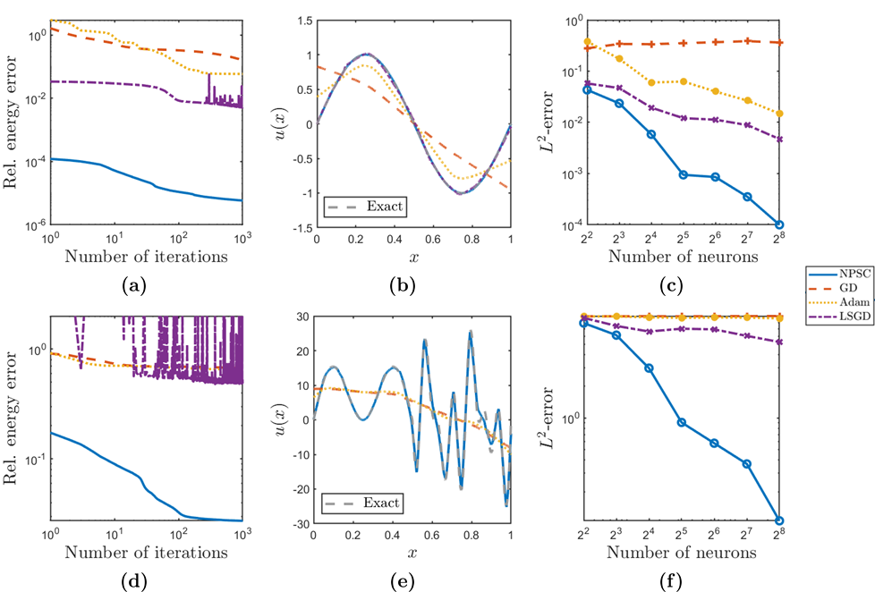
Figure 3: Numerical results for the function approximation problems (a–c) (29) and (d–f) (30). (a, d) Decay of the relative energy error $\frac{E(\theta^{(k)})-E^{*}}{|E^{*}|}$ in various training algorithms ($n=2^{5}$). (b, e) Exact solution and its approximations ($n=2^{5}$, $10^{3}$ epochs). (c, f) $L^{2}$-errors with respect to the number of neurons ($10^{3}$ epochs). The dotted line represents the theoretical optimal approximation rate.

If we set (4) in (3), then we obtain the $L^{2}$-function approximation problem, which is the most elementary instance of (3). That is, the solution of (3) in this case is the best $L^{2}$-approximation of $f$ found in $\Sigma_{n}$.

Test 1. As our first example, we consider $L^{2}$-approximation (4) for a sine function; we set

(29) $$\Omega=(0,1)\subset\mathbb{R},\quad f(x)=\sin 2\pi x$$

in (3). For numerical integration, we use the trapezoidal rule on 10,000 uniformly sampled points; see Appendix C. Fig. 3(a) plots the relative energy errors $\frac{E(\theta^{(k)})-E^{*}}{|E^{*}|}$ obtained by NPSC, GD, Adam, and LSGD per epoch, where $E^{*}$ is the loss corresponding to the exact solution. It is clear from the loss decay that NPSC outperforms all the other methods. The exact solution of (29) and its approximations obtained by $10^{3}$ epochs of the training algorithms with $2^{5}$ neurons are depicted in Fig. 3(b). One can readily observe that the NPSC result is most accurate among the approximations. The $L^{2}$-errors between the exact solution and its approximations for various numbers of neurons are presented in Fig. 3(c). Only the NPSC result seems to be comparable to $O(n^{-2})$, the theoretical optimal rate derived in [30].

Test 2. We revisit (6) as the second example, a highly oscillatory instance of (4):

(30) $$\Omega=(0,1)\subset\mathbb{R},\quad f(x)=\begin{cases}10\left(\sin 2\pi x+\sin 6\pi x\right),&\quad\textrm{ if }0\leq x<\frac{1}{2},\\ 10\left(\sin 8\pi x+\sin 18\pi x+\sin 26\pi x\right),&\quad\textrm{ if }\frac{1}{2}\leq x\leq 1,\end{cases}$$

in which a similar problem appeared in [6]. We note that it was demonstrated in [17] that training for complex functions like (30) is a much harder task than training for simple functions. Same as in (29), we use the trapezoidal rule on 10,000 uniformly sampled points for numerical integration. Fig. 3(d–f) present numerical results for the problem (30). In Fig. 3(d), NPSC shows stable decay of the loss while the losses of GD and Adam are stagnant along the epochs and that of LSGD blows up at in the beginning epochs and varies very rapidly. In Fig. 3(e), one can observe that the NPSC result captures both low- and high-frequency parts of the target function well, while the other ones captures the low-frequency part only [39]. Moreover, as shown in Fig. 3(f), the $L^{2}$-error of the NPSC decreases when the number of neurons increases, while those of the other algorithms seem to stagnate. This highlights the robustness of NPSC for complex problems.

5.2 Elliptic PDEs

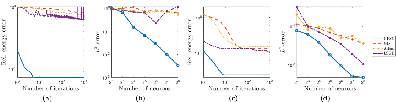
Figure 4: Numerical results for the elliptic PDEs (a, b) (32) and (c, d) (33). (a, c) Decay of the relative energy error $\frac{E(\theta^{(k)})-E^{*}}{|E^{*}|}$ in various training algorithms ($n=2^{5}$). (b, d) $L^{2}$-errors with respect to the number of neurons ($10^{3}$ epochs). The dotted line represents the theoretical optimal approximation rate.

Next, we consider the case

(31) $$V=H^{1}(\Omega),\quad a(u,v)=\int_{\Omega}\left(\nabla u\cdot\nabla v+uv\right)\,dx,\quad u,v\in V$$

in the problem (3), where $H^{1}(\Omega)$ is the usual Sobolev space consisting of $L^{2}(\Omega)$-functions with square-integrable gradients. It is well-known that (3) becomes the Galerkin approximation of the weak formulation of the following elliptic PDE on $\Sigma_{n}$ [38]:

$$-\Delta u+u=f\quad\text{ in }\Omega,\quad\frac{\partial u}{\partial n}=0\quad\text{ on }\partial\Omega,$$

where $\partial u/\partial n$ denotes the normal derivative of $u$ to $\partial\Omega$. Hence, one can find a numerical approximation for the solution of the above PDE by solving (31).

Test 1. In this test, we set

(32) $$\Omega=(0,1)\subset\mathbb{R},\quad f(x)=(1+9\pi^{2})\cos 3\pi x+(1+121\pi^{2})\cos 11\pi x$$

in (31). The exact solution is $u(x)=\cos 3\pi x+\cos 11\pi x$. We can observe in Fig. 4(a) that NPSC achieves a superior level of accuracy such that the other algorithms do not reach even with a large number of epochs. As shown in Fig. 4(b), $L^{2}$–errors of the NPSC results decrease as the number of neuron increases, and their decreasing rates are comparable to the theoretical optimal rates in [30].

Test 2. Finally, we consider the following two-dimensional example for (31):

(33) $$\Omega=(0,1)^{2}\subset\mathbb{R}^{2},\quad f(x_{1},x_{2})=(1+2\pi^{2})\cos\pi x_{1}\cos\pi x_{2},$$

whose exact solution is $u(x_{1},x_{2})=\cos\pi x\cos\pi y$. Since the preconditioner in Theorem 3.3 is applicable for one dimension only, in this example, $a$-minimization problems are solved by $n$ iterations of the unpreconditioned conjugate gradient method. We use the quasi-Monte Carlo method [5] with 10,000 sampling points for numerical integration; see Appendix C for details. It is verified by the numerical results for (33) presented in Fig. 4(c, d) that NPSC outperforms the other methods and provides reasonable $L^{2}$-errors in high-dimensional problems as well.

Remark 5.1.

When we train a neural network (2) for solving the PDE (31) with a gradient-based method, we have to evaluate the second-order derivative of $\sigma(x)$, which is the Dirac delta function. In our experiments, we simply ignore Dirac delta terms in numerical integration. This motivates us to consider high-order activation functions like ReLU^k [28] as a future work.

5.3 Ablation studies

We also validate the key components of the proposed NPSC method, namely, the optimal preconditioner for the linear layer (Theorem 3.3), the Levenberg–Marquardt algorithm for $\{\omega_{i},b_{i}\}$-minimization problems, the adjustment step for parameters (Algorithm 2), and the backtracking scheme for learning rates (Algorithm 3) by conducting ablation studies. The numerical results are discussed in Appendix B.

6 Conclusion

In this paper, we proposed NPSC for the finite neuron method with ReLU neural networks. Separately designing efficient solvers for the linear layer and each neuron and training them alternately, NPSC yields accurate results for function approximation problems and PDEs. With the NPSC method, one can separately design solvers for the linear and nonlinear layers. We note that, while the proposed optimal preconditioner is only available for one-dimensional problems, the parallel neuron-wise optimization of parameters in the nonlinear layer is not limited by dimensions.

6.1 Limitations and future directions

This paper leaves us several interesting and important topics for future research. Although NPSC adopts the well-established framework of subspace correction methods, its rigorous convergence analysis is still open due to the nonconvexity of the model. To solve high-order PDEs, we should generalize NPSC so that it can be applied to different kinds of activation functions or deep neural networks. In addition, designing optimal preconditioners for optimizing the linear layer in high dimensions is still open, which is considered as a much more challenging work than that in one dimension.

Appendix A Implementation details for the optimal preconditioner

In this appendix, we discuss the computational aspects of the proposed preconditioner. Although the preconditioner $P$ defined in (21) seems a bit complicated at the first glance, its computation requires only a cheap cost. We provide a detailed explanation of how to apply the preconditioner $P$ efficiently.

Three nontrivial parts in the preconditioner $P$ are the inverses of the matrices $B_{1}$, $\overline{K}_{\phi}$, and $R\overline{P}^{-1}R^{\mathrm{T}}$. First, we consider how to compute $B_{1}^{-1}\alpha$ when a vector $\alpha\in\mathbb{R}^{n_{\Omega}+2}$ is given. We solve a linear system $B_{1}\beta=\alpha$ in order to obtain $B_{1}^{-1}\alpha$. Thanks to the sparsity pattern of $B_{1}$, this linear system can be solved directly by the following $O(n)$ elementary arithmetic operations:

$$\beta_{i}=\begin{cases}\dfrac{1}{(B_{1})_{ii}}\left(\alpha_{i}-\dfrac{(B_{1})_{i,n_{\Omega}+1}}{(B_{1})_{n_{\Omega}+1,n_{\Omega}+1}}\alpha_{n_{\Omega}+1}-\dfrac{(B_{1})_{i,n_{\Omega}+2}}{(B_{1})_{n_{\Omega}+2,n_{\Omega}+2}}\alpha_{n_{\Omega}+2}\right),&\text{if }1\leq i\leq n_{\Omega},\\ \dfrac{\alpha_{i}}{(B_{1})_{ii}},&\text{otherwise.}\end{cases}$$

Secondly, we consider how to compute $\overline{K}_{\phi}^{-1}\alpha$ when a vector $\alpha\in\mathbb{R}^{n_{\Omega}+2}$ is given. In most applications, the bilinear form $a(\cdot,\cdot)$ is defined in terms of differential operators as in (31). This implies that the matrix $\overline{K}_{\phi}$ is tridiagonal, so that $\overline{K}_{\phi}^{-1}\alpha$ can be obtained by the Thomas algorithm (see, e.g., [13, Section 9.6]), which requires only $O(n)$ elementary arithmetic operations.

Finally, we discuss how to compute $(R\overline{P}^{-1}R^{\mathrm{T}})^{-1}\alpha$ for $\alpha\in\mathbb{R}^{n}$. Similarly, one can compute it by solving a linear system

$$R\overline{P}^{-1}R^{\mathrm{T}}\beta=\alpha.$$

By the definition (13) of $R$, we have

$$\overline{P}^{-1}R^{\mathrm{T}}\beta=\begin{bmatrix}\alpha_{1:n_{\Omega}}\\ \gamma\end{bmatrix}$$

for some $\gamma\in\mathbb{R}^{2}$, where $1:n_{\Omega}$ means “from the first to $n_{\Omega}$th entries.” One can readily deduce that $\gamma$ is determined by the following two relations:

(34a) $$\widetilde{R}\gamma=\alpha_{(n_{\Omega}+1):n},$$

(34b) $$\left(\overline{P}\begin{bmatrix}\alpha_{1:n_{\Omega}}\\ \gamma\end{bmatrix}\right)_{(n_{\Omega}+1):(n_{\Omega}+2)}\in\operatorname{ran}\widetilde{R}^{\mathrm{T}}.$$

Now, $\beta$ is then given by

$$\beta_{1:n_{\Omega}} =\left(\overline{P}\begin{bmatrix}\alpha_{1:n_{\Omega}}\\ \gamma\end{bmatrix}\right)_{1:n_{\Omega}},$$

$$\widetilde{R}^{\mathrm{T}}\beta_{(n_{\Omega}+1):n} =\left(\overline{P}\begin{bmatrix}\alpha_{1:n_{\Omega}}\\ \gamma\end{bmatrix}\right)_{(n_{\Omega}+1):(n_{\Omega}+2)}.$$

Since $\widetilde{R}\in\mathbb{R}^{(n-n_{\Omega})\times 2}$, (34a) and (34b) are written as $n-n_{\Omega}$ and $2-(n-n_{\Omega})$ linear equations, respectively. That is, $\gamma$ can be determined by solving the system (34) of two linear equations.

We now deal with how to solve the linear system (34) algebraically in detail. We write $\gamma=[\gamma_{1},\gamma_{2}]^{\mathrm{T}}\in\mathbb{R}^{2}$. By (9b), the number of interior nodal points $n_{\Omega}$ is either $n-2$, $n-1$, or $n$. First, we consider the case $n_{\Omega}=n-2$. In this case, (34b) obviously holds and (34a) reads as

(35a) $$\psi_{n_{\Omega}+1}(1)\gamma_{1}+\psi_{n_{\Omega}+1}(0)\gamma_{2} =\alpha_{n_{\Omega}+1},$$

(35b) $$\psi_{n_{\Omega}+2}(1)\gamma_{1}+\psi_{n_{\Omega}+2}(0)\gamma_{2} =\alpha_{n_{\Omega}+2}.$$

Hence, one can find $\gamma$ by solving (35) directly.

Next, we assume that $n_{\Omega}=n-1$. Then (34a) and (34b) read as (35a) and

(36) $$\overline{P}_{(n_{\Omega}+1):(n_{\Omega}+2),1:n_{\Omega}}\alpha_{1:n_{\Omega}}+\overline{P}_{(n_{\Omega}+1):(n_{\Omega}+2),(n_{\Omega}+1):(n_{\Omega}+2)}\gamma\in\operatorname{span}\left\{\begin{bmatrix}\psi_{n_{\Omega}+1}(1)\\ \psi_{n_{\Omega}+1}(0)\end{bmatrix}\right\},$$

respectively. Since (36) is equivalent to

(37) $$\left(\overline{P}_{n_{\Omega}+1,1:n_{\Omega}}\alpha_{1:n_{\Omega}}+\overline{P}_{n_{\Omega}+1,(n_{\Omega}+1):(n_{\Omega}+2)}\gamma\right)\psi_{n_{\Omega}+1}(0)\\ -\left(\overline{P}_{n_{\Omega}+2,1:n_{\Omega}}\alpha_{1:n_{\Omega}}+\overline{P}_{n_{\Omega}+2,(n_{\Omega}+1):(n_{\Omega}+2)}\gamma\right)\psi_{n_{\Omega}+1}(1)=0,$$

$\gamma$ can be obtained by solving the linear system consisting of (35a) and (37).

Finally, we consider the case $n_{\Omega}=n$. In this case, (34a) is void and (34b) reads as

$$\overline{P}_{(n_{\Omega}+1):(n_{\Omega}+2),1:n_{\Omega}}\alpha_{1:n_{\Omega}}+\overline{P}_{(n_{\Omega}+1):(n_{\Omega}+2),(n_{\Omega}+1):(n_{\Omega}+2)}\gamma =0.$$

Therefore, $\gamma$ is found by solving the above linear system.

In summary, the optimal preconditioner requires only $O(n)$ elementary arithmetic operations.

Appendix B Numerical results for the ablation studies

In this appendix, we discuss the numerical results of the ablation studies for the proposed NPSC method.

B.1 Effect of preconditioning

$n$	Problem (30)		Problem (32)
	Prec.	Unprec.	Prec.	Unprec.
$2^{4}$	2	34	3	19
$2^{5}$	2	107	2	37
$2^{6}$	2	310	4	59
$2^{7}$	3	1018	4	103
$2^{8}$	3	3470	5	173

Table 1: Number of preconditioned and unpreconditioned conjugate gradient iterations to solve the $a$-minimization problems (7) corresponding to the $L^{2}$-function approximation problem (30) and the elliptic PDE (32), where $n$ denotes the number of neurons.

We present some numerical results to highlight the computational efficiency of the preconditioner $P$. The $a$-minimization problems (24) appearing in training of neural networks that solve the $L^{2}$-function approximation problem (30) and the elliptic boundary value problem (32) are considered. We set the parameters $\omega$ and $b$ in the nonlinear layer as follows:

$$\omega_{i}=1,\quad b_{i}=-\frac{i}{n+1},\quad 1\leq i\leq n.$$

We compare the numerical performances of the preconditioned and unpreconditioned conjugate gradient methods solving (24). The initial guess $a^{(0)}$ is given by the zero vector. Table 1 presents the number of iterations of the preconditioned and unpreconditioned conjugate gradient methods to meet the stop condition (28) with respect to various numbers of neurons $n$. While the number of unpreconditioned iterations increases rapidly as $n$ increases, the number of preconditioned iterations is uniformly bounded with respect to $n$. This supports our theoretical result presented in Theorem 3.3, which claims that the condition number of the preconditioned operator $PK$ is $O(1)$. Since the computational cost of $P$ is cheap, we can conclude that the preconditioner $P$ is numerically efficient.

B.2 Effect of backtracking for conventional training algorithms

We present numerical results that show that the backtracking scheme presented in Algorithm 3 is useful not only for the proposed NPSC but also for conventional training algorithms such as GD, Adam [15], and LSGD [9].

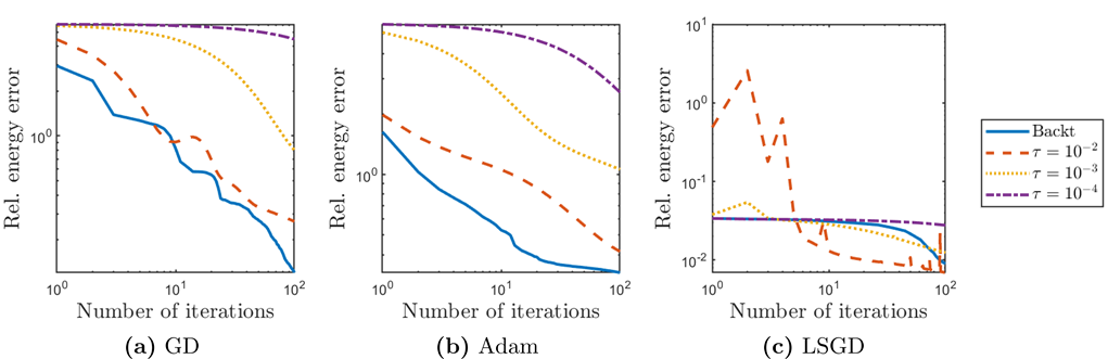
Figure 5: Decay of the relative energy error $\frac{E(\theta^{(k)})-E^{*}}{|E^{*}|}$ in various training algorithms for solving (29). “Backt” denotes the backtracking scheme presented in Algorithm 3, and $\tau$ denotes the fixed learning rate.

Fig. 5 plots the relative energy error $\frac{E(\theta^{(k)})-E^{*}}{|E^{*}|}$ of GD, Adam, and LSGD for solving the problem (29), averaged over 10 random initializations, where $k$ denotes the number of epochs and $E^{*}$ is the energy corresponding to the exact solution of the problem. The number of neurons used is $2^{5}$; while we can observe similar results for the other numbers of neurons, we only provide the result of $2^{5}$ neurons for brevity. We observe that the algorithms equipped with the backtracking scheme outperform those with constant learning rates $\tau=10^{-2}$, $10^{-3}$, and $10^{-4}$ in the sense of the convergence rate. That is, Algorithm 3 seems to successfully find a good learning rate at each iteration of conventional training algorithms as well. Hence, in Section 5, we employ Algorithm 3 to find learning rates of GD, Adam, and LSGD.

B.3 Effect of parameter adjustment and Levenberg-Marquardt algorithm

Fig. 6 depicts numerical comparisons among three algorithms: NPSC, NPSC without Algorithm 2 (parameter adjustment), and NPSC without the Levenberg–Marquardt algorithm.

One can see the variants of NPSC achieve slower convergence rates than NPSC in all the examples. Therefore, both Algorithm 2 and the Levenberg–Marquardt algorithm contribute to the fast convergence of NPSC. We also note that Algorithm 2 helps NPSC to avoid unstable convergence behaviors like Fig. 6(c, d).

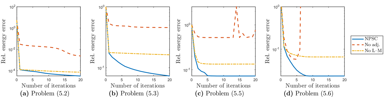
Figure 6: Ablation studies for NPSC on the relative energy error $\frac{E(\theta^{(k)})-E^{*}}{|E^{*}|}$. “No adj.” and “No L–M” denote NPSC without the adjustment step and the Levenberg–Marquardt algorithm, respectively.

Appendix C Numerical integration

This appendix is devoted to numerical integration schemes for computing the integral in our model problem (3). If $d=1$, i.e., if the domain $\Omega=(0,1)\subset\mathbb{R}$, then we approximate the integral of a function $g(x)$ defined on $\Omega$ by the following simple trapezoidal rule:

(38) $$\int_{\Omega}g(x)\,dx\approx\sum_{j=1}^{N-1}\frac{g(x_{j})+g(x_{j+1})}{2}(x_{j+1}-x_{j}),$$

where $0=x_{1}<x_{2}<\dots<x_{N}=1$ are $N$ uniform sampling points between $0$ and $1$, i.e., $x_{j}=\frac{j-1}{N-1}$, $1\leq j\leq N$. Approximation properties of the trapezoidal rule (38) can be found in standard textbooks on numerical analysis; see, e.g., [4].

When $d\geq 2$, we adopt the quasi-Monte Carlo method [5] based on Halton sequences [16], which is known to overcome the curse of dimensionality in the sense that approximation error bounds independent of the dimension $d$ are available. In the quasi-Monte Carlo method, the integral of a function $g(x)$ defined on $\Omega$ is approximated by the average of the function evaluated at $N$ sampling points:

(39) $$\int_{\Omega}g(x)\,dx\approx\frac{1}{N}\sum_{j=1}^{N}g(x_{j}),$$

where $\{x_{j}\}_{j=1}^{N}$ is a low-discrepancy sequence in $\Omega$ defined in terms of Halton sequences. For the sake of description, we assume that $\Omega=(0,1)^{d}\in\mathbb{R}^{d}$. Then the $k$th coordinate of $x_{j}$ ($1\leq j\leq N$, $1\leq k\leq d$) is the number $j$ written in $p_{k}$-ary representation, inverted, and written after the decimal point, where $p_{k}$ is the $k$th smallest prime number. For example, if $d=3$, then the first four points of $\{x_{j}\}_{j=1}^{N}$ is given by

$$x_{1}=\left(\frac{1}{2},\frac{1}{3},\frac{1}{5}\right),\hskip 2.84544ptx_{2}=\left(\frac{1}{2^{2}},\frac{2}{3},\frac{2}{5}\right),\hskip 2.84544ptx_{3}=\left(\frac{3}{2^{2}},\frac{1}{3^{2}},\frac{3}{5}\right),\hskip 2.84544ptx_{4}=\left(\frac{1}{2^{3}},\frac{4}{3^{2}},\frac{4}{5}\right).$$

Approximation properties of (39) can be found in [5].

References

- [1] M. Ainsworth and Y. Shin, Plateau phenomenon in gradient descent training of ReLU networks: Explanation, quantification, and avoidance, SIAM J. Sci. Comput., 43 (2021), pp. A3438–A3468.
- [2] M. Ainsworth and Y. Shin, Active Neuron Least Squares: A training method for multivariate rectified neural networks, SIAM J. Sci. Comput., 44 (2022), pp. A2253–A2275.
- [3] L. Badea and R. Krause, One-and two-level Schwarz methods for variational inequalities of the second kind and their application to frictional contact, Numer. Math., 120 (2012), pp. 573–599.
- [4] R. L. Burden, J. D. Faires, and A. M. Burden, Numerical Analysis, Cengage Learning, Boston, MA, 2015.
- [5] R. E. Caflisch, Monte Carlo and quasi-Monte Carlo methods, Acta Numer., 7 (1998), pp. 1–49.
- [6] W. Cai, X. Li, and L. Liu, A phase shift deep neural network for high frequency approximation and wave problems, SIAM J. Sci. Comput., 42 (2020), pp. A3285–A3312.
- [7] L. Calatroni and A. Chambolle, Backtracking strategies for accelerated descent methods with smooth composite objectives, SIAM J. Optim., 29 (2019), pp. 1772–1798.
- [8] G. Cybenko, Approximation by superpositions of a sigmoidal function, Math. Control Signals Syst., 2 (1989), pp. 303–314.
- [9] E. C. Cyr, M. A. Gulian, R. G. Patel, M. Perego, and N. A. Trask, Robust training and initialization of deep neural networks: An adaptive basis viewpoint, in Proceedings of The First Mathematical and Scientific Machine Learning Conference, vol. 107 of Proceedings of Machine Learning Research, PMLR, 2020, pp. 512–536.
- [10] W. E and B. Yu, The deep Ritz method: a deep learning-based numerical algorithm for solving variational problems, Commun. Math. Stat., 6 (2018), pp. 1–12.
- [11] J. He, L. Li, J. Xu, and C. Zheng, ReLU deep neural networks and linear finite elements, J. Comput. Math., 38 (2020), pp. 502–527.
- [12] K. He, X. Zhang, S. Ren, and J. Sun, Delving deep into rectifiers: Surpassing human-level performance on ImageNet classification, in Proceedings of the IEEE International Conference on Computer Vision, 2015, pp. 1026–1034.
- [13] N. J. Higham, Accuracy and Stability of Numerical Algorithms, SIAM, Philadelphia, PA, second ed., 2002.
- [14] Q. Hong, J. W. Siegel, Q. Tan, and J. Xu, On the activation function dependence of the spectral bias of neural networks, arXiv preprint arXiv:2208.04924, (2022).
- [15] D. P. Kingma and J. Ba, Adam: A method for stochastic optimization, in 3rd International Conference on Learning Representations, ICLR 2015, San Diego, CA, USA, May 7-9, 2015, Conference Track Proceedings, 2015.
- [16] L. Kocis and W. J. Whiten, Computational investigations of low-discrepancy sequences, ACM Trans. Math. Software, 23 (1997), pp. 266–294.
- [17] A. Krishnapriyan, A. Gholami, S. Zhe, R. Kirby, and M. W. Mahoney, Characterizing possible failure modes in physics-informed neural networks, in Advances in Neural Information Processing Systems, vol. 34, Curran Associates, Inc., 2021, pp. 26548–26560.
- [18] C.-O. Lee and J. Park, Fast nonoverlapping block Jacobi method for the dual Rudin–Osher–Fatemi model, SIAM J. Imaging Sci., 12 (2019), pp. 2009–2034.
- [19] D. W. Marquardt, An algorithm for least-squares estimation of nonlinear parameters, J. Soc. Ind. Appl. Math., 11 (1963), pp. 431–441.
- [20] J. Nocedal and S. J. Wright, Numerical Optimization, Springer, New York, second ed., 2006.
- [21] H. Park, S.-I. Amari, and K. Fukumizu, Adaptive natural gradient learning algorithms for various stochastic models, Neural Netw., 13 (2000), pp. 755–764.
- [22] J. Park, Additive Schwarz methods for convex optimization as gradient methods, SIAM J. Numer. Anal., 58 (2020), pp. 1495–1530.
- [23] J. Park, Additive Schwarz methods for convex optimization with backtracking, Comput. Math. Appl., 113 (2022), pp. 332–344.
- [24] A. Pinkus, Approximation theory of the MLP model in neural networks, Acta Numer., 8 (1999), pp. 143–195.
- [25] M. Raissi, P. Perdikaris, and G. E. Karniadakis, Physics-informed neural networks: A deep learning framework for solving forward and inverse problems involving nonlinear partial differential equations, J. Comput. Phys., 378 (2019), pp. 686–707.
- [26] Y. Saad, Iterative Methods for Sparse Linear Systems, SIAM, Philadelphia, 2003.
- [27] K. Scheinberg, D. Goldfarb, and X. Bai, Fast first-order methods for composite convex optimization with backtracking, Found. Comput. Math., 14 (2014), pp. 389–417.
- [28] J. W. Siegel and J. Xu, High-order approximation rates for shallow neural networks with cosine and ReLUk activation functions, Appl. Comput. Harmon. Anal., 58 (2022), pp. 1–26.
- [29] J. W. Siegel and J. Xu, Optimal convergence rates for the orthogonal greedy algorithm, IEEE Trans. Inform. Theory, 68 (2022), pp. 3354–3361.
- [30] J. W. Siegel and J. Xu, Sharp bounds on the approximation rates, metric entropy, and -widths of shallow neural networks, Found. Comput. Math., (2022), https://doi.org/10.1007/s10208-022-09595-3.
- [31] M. Soltanolkotabi, Learning ReLUs via gradient descent, in Advances in Neural Information Processing Systems, vol. 30, 2017.
- [32] X.-C. Tai and J. Xu, Global and uniform convergence of subspace correction methods for some convex optimization problems, Math. Comp., 71 (2002), pp. 105–124.
- [33] Y. Tian, An analytical formula of population gradient for two-layered ReLU network and its applications in convergence and critical point analysis, in Proceedings of the 34th International Conference on Machine Learning, vol. 70, PMLR, 2017, pp. 3404–3413.
- [34] A. Toselli and O. Widlund, Domain Decomposition Methods—Algorithms and Theory, Springer, Berlin, 2005.
- [35] G. Vardi, G. Yehudai, and O. Shamir, Learning a single neuron with bias using gradient descent, in Advances in Neural Information Processing Systems, vol. 34, 2021.
- [36] S. J. Wright, Coordinate descent algorithms, Math. Program., 151 (2015), pp. 3–34.
- [37] J. Xu, Iterative methods by space decomposition and subspace correction, SIAM Rev., 34 (1992), pp. 581–613.
- [38] J. Xu, Finite neuron method and convergence analysis, Commun. Comput. Phys., 28 (2020), pp. 1707–1745.
- [39] Z.-Q. J. Xu, Y. Zhang, T. Luo, Y. Xiao, and Z. Ma, Frequency principle: Fourier analysis sheds light on deep neural networks, Commun. Comput. Phys., 28 (2020), pp. 1746–1767.
- [40] N. Yamashita and M. Fukushima, On the rate of convergence of the Levenberg-Marquardt method, in Topics in Numerical Analysis, vol. 15 of Comput. Suppl., Springer, Vienna, 2001, pp. 239–249.
- [41] G. Yehudai and O. Shamir, Learning a single neuron with gradient methods, in Proceedings of Thirty Third Conference on Learning Theory, vol. 125 of Proceedings of Machine Learning Research, PMLR, 2020, pp. 3756–3786.
- [42] J. Zeng, T. T.-K. Lau, S. Lin, and Y. Yao, Global convergence of block coordinate descent in deep learning, in Proceedings of the 36th International Conference on Machine Learning, vol. 97, PMLR, 2019, pp. 7313–7323.
- [43] Z. Zhang and M. Brand, Convergent block coordinate descent for training Tikhonov regularized deep neural networks, in Advances in Neural Information Processing Systems, vol. 30, Curran Associates, Inc., 2017.