PhAST: Physics-Aware, Scalable, and Task-Specific GNNs for Accelerated Catalyst Design

Mitigating the climate crisis requires a rapid transition towards lower-carbon energy. Catalyst materials play a crucial role in the electrochemical reactions involved in numerous industrial processes key to this transition, such as renewable energy storage and electrofuel synthesis. To reduce the energy spent on such activities, we must quickly discover more efficient catalysts to drive electrochemical reactions. Machine learning (ML) holds the potential to efficiently model materials properties from large amounts of data, accelerating electrocatalyst design. The Open Catalyst Project OC20 dataset was constructed to that end. However, ML models trained on OC20 are still neither scalable nor accurate enough for practical applications. In this paper, we propose task-specific innovations applicable to most architectures, enhancing both computational efficiency and accuracy. This includes improvements in (1) the graph creation step, (2) atom representations, (3) the energy prediction head, and (4) the force prediction head. We describe these contributions and evaluate them thoroughly on multiple architectures. Overall, our proposed PhAST improvements increase energy MAE by 4 to 42$\%$ while dividing compute time by 3 to 8$\times$ depending on the targeted task/model. PhAST also enables CPU training, leading to 40$\times$ speedups in highly parallelized settings. Python package: https://phast.readthedocs.io.

Keywords: climate change, scientific discovery, material modeling, graph neural networks, electrocatalysts.

1 Introduction

To mitigate climate change at a global scale, it is imperative to reduce the carbon emissions of ubiquitous industrial processes like cement production or fertiliser synthesis, as well as to develop infrastructures for storing low-carbon energy at scale, enabling to re-use it wherever and whenever needed. Since such processes rely on electrochemical reactions, they require the design of more efficient electrocatalysts (Zakeri and Syri, 2015) to become more environmentally and economically viable.

However, discovering easy-to-exploit low-cost catalysts that drive electrochemical reactions at high rates remains an open challenge. In fact, today’s catalyst discovery pipeline mostly relies on expensive quantum mechanical simulations such as the Density Functional Theory (DFT) to approximate the behaviour of the materials involved in the targeted chemical reaction. Unfortunately, the high computational cost of these simulations limits the number of candidates that can be efficiently tested, and consequently stagnates further advances in the field.

Machine learning (ML) holds the potential to approximate these calculations while reducing the time needed to assess each candidate by several orders of magnitude (Zitnick et al., 2020). This capability could transform the search for new catalysts, by making it possible to sort through millions or even billions of possible materials to identify promising candidates for experimental inquiry(Zitnick et al., 2020).

To enable to use of ML for catalyst discovery, the Open Catalyst Project released OC20 (Chanussot et al., 2021), a large data set of pairs of catalyst and target molecule (known as adsorbate), along with the relaxed energy of the resulting system—a relevant metric to assess how good a catalyst is for a given chemical reaction—computed with DFT from the initial atomic structure. Despite recent progress (Gasteiger et al., 2021; Ying et al., 2021), major challenges remain. First, state-of-the-art models have not yet reached high enough performance for practical applications. Second, they are still too computationally expensive to allow the millions of inferences required to explore the large space of potential catalysts. Third, the graph neural networks (GNNs) typically used are designed for general 3D material modeling tasks rather than specifically for catalyst discovery, a complex task that may benefit from domain-specific architectures.

To address these challenges, we propose multiple model improvements to increase the accuracy and scalability of generic GNNs applied to catalyst discovery. In particular, our contributions are (1) a graph construction that is tailored to catalyst-adsorbate modeling, (2) richer physics-based atom representations, (3) an energy head that learns a weighted sum of per-atom predictions, and (4) a direct force prediction head encouraging energy conservation. We provide a broad evaluation of these contributions on OC20 and a thorough ablation study. In sum, the proposed PhAST improvements increase energy MAE by 5–42 % while dividing compute time by 3–8$\times$ depending on the targeted task/model. These gains in model scalability enable efficient CPU training, with up to 40$\times$ speedups in highly parallelized pipelines using PhAST, making these models significantly more accessible to a wider community of researchers. We also believe that our work provides valuable insights for future research as it leverages domain-specific knowledge to improve parts of the pipeline that were not investigated up to now. Overall, the resulting performance and scalability gains open the door to a practical use of GNNs for new electrocatalyst design, the ultimate end goal of this line of research.

2 Background

The problem we address is the prediction of the relaxed energy $y\in{\mathbb{R}}$ of an adsorbate-catalyst system from its initial configuration in space $({\boldsymbol{X}},{\boldsymbol{Z}})$, where ${\boldsymbol{X}}\in{\mathbb{R}}^{N\times 3}$ is the matrix of 3D atom positions and ${\boldsymbol{Z}}\in\mathbb{N}^{N}$ contains atom characteristic numbers. This task is referred to as Initial Structure to Relaxed Energy, IS2RE, in Zitnick et al. (2020). This is commonly formulated as a graph regression task, where each sample is represented as a 3D graph ${\mathcal{G}}$ with node set $\mathcal{V}$ of dimension $N$ and adjacency matrix ${\boldsymbol{A}}\in{\mathbb{R}}^{N\times N}$. ${\boldsymbol{H}}\in{\mathbb{R}}^{N\times H}$ represents atom embeddings and ${\boldsymbol{T}}\in\{0,1,2\}^{N}$ corresponds to tag information (see 3.1). ML models designed for this task generally adopt graph neural networks as an architecture, as it naturally suits 3D material modeling. Such GNNs typically share a common pipeline for how they are applied, as depicted in Fig. 1.

Figure 1: Common GNN inference pipeline for 3D material modeling. The graph creation step remains unchanged across all methods: it creates ${\boldsymbol{A}}$ using cutoff distances and periodic boundary conditions. The Embedding and Output blocks slightly differ across models but the underlying idea is the same. The Embedding block learns a representation for each chemical element and the Output block applies a global pooling of each node’s representation to obtain the energy prediction. The key distinction between methods typically lies in the Interaction block, where the message passing schemes vary.

In material modeling tasks, it is desirable to endow ML models with relevant symmetry properties. In particular, we want predictions to be equivariant to translations, rotations and (often) reflections. Many models enforce these physical priors within the architecture, making it explicitly invariant or equivariant to the desired transformations. Formal definitions are included in Section A.1.

Many GNNs in prior work focus on enforcing equivariance, though it is not strictly required for relaxed energy prediction, which calls for invariance. Equivariant GNNs (Thomas et al., 2018; Anderson et al., 2019; Fuchs et al., 2020; Batzner et al., 2022; Brandstetter et al., 2021) are expressive and generalize well, but are very computationally expensive as they are constrained by equivariant filters built on spherical harmonics and the Clebsch-Gordan tensor product. Recent methods  (Schütt et al., 2021; Satorras et al., 2021; Thölke and De Fabritiis, 2022) model equivariant interactions in Cartesian space using both invariant (scalar) and vector representations. While they are faster, their architectures are often very complex and lack theoretical guarantees. Alternatively, E(3)-invariant methods (Schütt et al., 2017; Unke and Meuwly, 2019; Shuaibi et al., 2021; Ying et al., 2021; Adams et al., 2021; Zitnick et al., 2022) do not use atom positions directly in their internal workings. Instead, these methods extract and use quantities that remain invariant under rotations and reflections. DimeNet++ (Klicpera et al., 2020b, a), for example, includes a directional message passing (MP) mechanism that incorporates bond angles in addition to atom relative distances. However, distances and bond angles do not suffice to uniquely identify the graph 3D structure. This is achieved by SphereNet (Liu et al., 2021) and GemNet (Gasteiger et al., 2021), which additionally extract torsion information (between quadruplets of nodes). On the downside, these methods are very computationally expensive as they require considering 3-hop neighbourhoods for each update step. Importantly, all these Message Passing methods aim at broad applicability and do not leverage the specific constraints of individual tasks.

3 Proposed Method

In this section, we describe PhAST, a Physics-Aware, Scalable, and Task-specific GNN framework for catalyst design. Notably, the architectural innovations in our proposed framework are applicable to most current GNNs used in materials discovery. These include a novel graph creation step, richer atom representations, an advanced energy head for graph-level prediction, and a direct (energy-conserving) force-head for atom-wise predictions.

3.1 Graph creation

Although the graph construction step is critical in graph ML tasks, it has received little or no attention by previous work on the OC20 data set. Most methods reuse the original proposal by Chanussot et al. (2021). In OC20, each graph’s atom is tagged as part of the adsorbate (tag 2), the catalyst’s surface (tag 1), or its sub-surface volume (tag 0). Tag 0 atoms were originally added in DFT simulations to represent more explicitly the repeating pattern of the catalyst slab. They are, by definition, further away from the adsorbate and are fixed by construction, unlike tag 1 and tag 2 atoms, which can move during the relaxation. As a result, we hypothesise they contain redundant information, making them of lesser importance to predict the final relaxed energy. Besides, since they account for $\sim 65\%$ of the nodes B.5, and since SOTA GNNs often depend on multiple hops to compute bond and torsion angles, we propose to remove these nodes from the graph. This should greatly reduce inference time without impacting expressivity. As an alternative intermediate approach, we explore forming super nodes that aggregate tag 0 atoms to avoid a potential information loss caused by their total removal. We briefly describe these changes below, with more details in Section A.2.

remove-tag-0 removes all atoms with tag 0 (i.e. in $\mathcal{S}=\{i\in\mathcal{V}:t_{i}=0\}$) from the graph, adapting correspondingly all graph attributes (${\boldsymbol{X}}$, ${\boldsymbol{A}}$, ${\boldsymbol{Z}}$, ${\boldsymbol{T}}$, etc.).

one-supernode-per-graph aggregates all tag 0 nodes from ${\mathcal{G}}$ into a supernode $s$ with position ${\boldsymbol{x}}_{s}=\frac{{\boldsymbol{X}}_{\mathcal{S}}1}{|{\mathcal{S}}|}\sum_{i\in{\mathcal{S}}}{\boldsymbol{x}}_{i}$, adjacency $A_{is}=\max(A_{ij}:j\in{\mathcal{S}})$ and a new characteristic number $z_{s}$.

one-supernode-per-atom-type replicates the above strategy but creates one super node per distinct chemical element in the catalyst subsurface. Its attributes are defined based on its components, as previously.

3.2 Atom Embeddings

In all previously proposed GNN methods to solve energy-prediction tasks (e.g. IS2RE), atom representations are learned from scratch based on atomic number ${\boldsymbol{H}}={\boldsymbol{H}}_{{\boldsymbol{Z}}}$. We propose to leverage domain information to improve these representations. First, we hypothesise that whether a given atom belongs to the adsorbate, the catalyst surface, or its subsurface is important information. We therefore incorporate tag information into our model by utilizing a learnable embedding matrix ${\boldsymbol{H}}_{{\boldsymbol{T}}}$ that encodes the tags as vectors. Second, we know from previous studies that some atomic properties (e.g. atomic radius or density) are useful for catalyst discovery (Takigawa et al., 2016; Ward et al., 2017). We leverage them as an additional embedding vector ${\boldsymbol{H}}_{\mathbf{F}}$ (see A.3 for the full list of properties). Lastly, we let the GNN learn embeddings for both the group and period information (${\boldsymbol{H}}_{\mathbf{P}},{\boldsymbol{H}}_{\mathbf{G}}$) since atoms belonging to the same group or period often share similar behaviours (Xie and Grossman, 2018). As a result, our proposed atom embedding ${\boldsymbol{H}}$ is a concatenation of all of the above: ${\boldsymbol{H}}={\boldsymbol{H}}_{Z}||{\boldsymbol{H}}_{T}||{\boldsymbol{H}}_{F}||{\boldsymbol{H}}_{P}||{\boldsymbol{H}}_{G}$.

3.3 Energy head

In the literature, there is often limited focus on the energy head, which is the part of the output block responsible for the energy computation from final atom representations ${\boldsymbol{h}}^{L}_{i}$. To the best of our knowledge, all GNNs compute the relaxed energy using global pooling $y=\sum_{i\in\mathcal{V}}h_{i}$, where node embeddings are reduced to a scalar $h_{i}$ by linear layers. We identify two limitations in this procedure: First, all atoms are assigned the same importance, even though the properties of an atom are normally influenced by the properties of the element. Second, the graph topology is neglected by simply summing all atom encodings regardless of their 3D positions. To overcome these limitations, we explore alternative energy heads.

First, a weighted sum of node representations, which grants adaptive importance to each chemical element, expressed as $\hat{y}=\sum_{i\in\mathcal{V}}\alpha({\boldsymbol{h}}^{L}_{i})\cdot h_{i}$ or $\hat{y}=\sum_{i\in\mathcal{V}}\alpha({\boldsymbol{h}}^{0}_{i})\cdot h_{i}$, where the learnable importance weights $\alpha(\cdot)$ depend either on the embedding block initial encodings ${\boldsymbol{h}}^{0}_{i}$ or final ones ${\boldsymbol{h}}^{L}_{i}$.

Second, a hierarchical pooling approach endowed with the following energy head pipeline: ${\boldsymbol{h}}^{L}_{i}\rightarrow$ [Pooling $\rightarrow$ GCN] ($\times 2$) $\rightarrow$ Global Pooling $\rightarrow$ MLP $\rightarrow\hat{y}$. By applying a graph convolutional network (GCN, Kipf and Welling, 2016) on a coarsened graph, we propagate information differently, allowing us to capture hierarchical graph information. We implement hoscpool (Duval and Malliaros, 2022): an end-to-end pooling operator that learns a cluster assignment matrix using a loss function inspired by motif spectral clustering.

3.4 Force head

A closely related task to IS2RE (i.e. energy prediction) consists in computing forces together with energy. This involves the additional prediction and training of atom-wise 3D vectors representing the forces currently applied on each atom by the rest of the system. This task is referred to as Structure to Energy and Forces, S2EF in Zitnick et al. (2020). In many previous works, atomic forces are directly computed as the predicted energy’s gradient with respect to atom positions $\vec{y}_{i}=\frac{\partial y}{\partial{\boldsymbol{x}}_{i}}$ (i.e. its definition in physics). While this guarantees energy-conserving forces, Kolluru et al. (2022) demonstrated the significant computational burden associated with this approach, which increases memory use by a factor of 2–4 and leads to decreased modeling performance for specific datasets. As a result, several recent works neglected this principle on OC20, proposing direct force predictions from final atom representations. Here, we extend this idea by proposing a plug-and-play force head architecture for traditional energy conserving GNNs (Schütt et al., 2017; Klicpera et al., 2020b). We thus use two independent output heads: $\Phi^{1}$ for graph-level energy predictions and $\Phi^{2}$ for atom-level force predictions. Since energy conservation remains desirable, we propose to strengthen this property by fine-tuning models on a gradient-target loss term: the $L_{2}$ (squared) distance between atomic force predictions and energy gradient with respect to atom positions:

$$\mathcal{L}_{EC}=\sum_{i}||\Phi^{2}_{F}(\mathcal{G})-\nabla\Phi^{1}_{F}(\mathcal{G})||_{2}^{2}.$$ (1)

Since this term may be redundant due to existing energy loss $\mathcal{L}_{E}=||\hat{y}-y||_{2}$ and force loss $\mathcal{L}_{F}=||\hat{\vec{y}}-\vec{y}||_{2}$, we also study the alternative use of a cosine similarity loss between predicted forces $\hat{\vec{y}}=\Phi^{2}_{F}(\mathcal{G})$ and ground truth ones $\vec{y}$ (for $\epsilon>0$):

$$\mathcal{L}_{EC}=\dfrac{\hat{\vec{y}}\cdot\vec{y}}{\max(\|\hat{\vec{y}}\|_{2}\cdot\|\vec{y}\|_{2},\epsilon)}.$$ (2)

3.5 PhAST: final components

In LABEL:sec:ablation, we present the ablation study that lead us to the selection of the various components that make PhAST. As an overview, we list them here:

1. Graph creation: remove-tag-0.

2. Atom embeddings: all embeddings ${\boldsymbol{H}}={\boldsymbol{H}}_{Z}||{\boldsymbol{H}}_{T}||{\boldsymbol{H}}_{F}||{\boldsymbol{H}}_{P}||{\boldsymbol{H}}_{G}$.

3. Energy head: weighted sum from initial embeddings.

4. Force head: direct force prediction with gradient target loss.

4 Evaluation

In this section, we evaluate the performance and scalability of the PhAST framework for five well-known GNNs on the OC20 dataset (Chanussot et al., 2021). We first perform an in-depth study of the first three components of PhAST on the OC20 IS2RE energy prediction task, before looking at the gains of the last component (i.e. the force head) on the OC20 S2EF-2M energy-force prediction task.

4.1 Baselines

We target five well-known GNN baselines to study the impact of our contributions. We have selected them based on their popularity and ease-of-implementation but note that PhAST improvements are applicable to all recent GNNs for 3D material modeling, to the best of our knowledge, because the changes are architecture-agnostic. We use the hyperparameters, training settings and model architectures provided in the original papers. As mentioned in Figure 1, they all follow a similar pipeline, mainly differing in their interaction blocks, which we briefly detail below.

SchNet (Schütt et al., 2017) is a simple message passing architecture that leverages relative distances to update atom representations via a continuous filter: ${\boldsymbol{h}}_{i}^{(l+1)}=\sum_{j}{\boldsymbol{h}}_{j}^{l}\odot W^{l}({\boldsymbol{x}}_{i}-{\boldsymbol{x}}_{j})$ where $W^{l}({\boldsymbol{x}}_{i}-{\boldsymbol{x}}_{j})$ is a radial basis function to encode distance between atom pairs.

DimeNet++ (Klicpera et al., 2020a) is an optimised version of DimeNet (Klicpera et al., 2020b), which proposes a directional message passing. In other words, they compute and update edge representations instead of atoms) using interatomic distances $\mathbf{e}_{RBF}$ (encoded via bessel functions) and bond angles $\mathbf{a}_{SBF}$ (encoded via 2D spherical Fourier-Bessel basis):

$$\mathbf{m}_{ij}^{(l+1)}=f_{update}\big{(}\mathbf{m}_{ij}^{(l)},\sum_{k\in N_{j}\setminus i}f_{int}(\mathbf{m}_{ij}^{(l)},\mathbf{e}_{RBF}^{(ij)},\mathbf{a}_{SBF}^{(ki,ji)})\big{)}$$

ForceNet (Hu et al., 2021) is a scalable force-centric GNN that does not impose explicit physical constraints (energy conservation, rotational invariance). It attempts to encourage invariance by efficient rotation-based data augmentation. Model-wise, it adopts a node message passing approach that leverages node positions directly via a spherical harmonics basis.

GemNet (Gasteiger et al., 2021) builds on top of DimeNet++, but additionally incorporates torsion information between quadruplets of atoms. This grants it the ability to process more geometric information and thus to distinguish between a wider range of different graphs, at the cost of extra computational cost and model complexity.

GemNet-OC (Gasteiger et al., 2022) is an improved version of GemNet.

4.2 PhAST performance on IS2RE

Dataset. OC20 contains 1,281,040 DFT relaxations of randomly selected catalysts and adsorbates from a set of plausible candidates. In this section, we focus on the Initial Structure to Relaxed Energy (IS2RE) task (Zitnick et al., 2020), that is the direct prediction of the relaxed adsorption energy from the initial atomic structure. It comes with a pre-defined train/val/test split, 450,000 training samples and hidden test labels. Experiments are evaluated on the validation set, which has four splits of $\sim 25K$ samples: In Domain (ID), Out of Domain adsorbates (OOD-ads), Out of Domain catalysts (OOD-cat), and Out of Domain adsorbates and catalysts (OOD-both).

Metrics. We measure accuracy via the energy Mean Average Error (MAE) in meV on each validation split, and scalability by the inference time (in seconds) over the whole ID validation set. We also include throughput in LABEL:app:tab:throughput-is2re, i.e. the number of samples processed per second at inference time. Since the absolute time metrics are difficult to compare across hardware setups with respect to other works, we note that the most relevant metrics are the relative improvements we show using the exact same hardware and software for all models. In order to easily visualize the contributions of PhAST on the baseline models in terms of performance improvement, in Figure 2 (left) we plot the relative MAE improvement with respect to the baseline. Specifically, we compute the MAE improvement as

$$\text{MAE improvement}=100\times\frac{\text{MAE(PhAST)}-\text{MAE(baseline)}}{\text{MAE(baseline)}}.$$ (3)

Baselines. We study the enhancements brought by the PhAST components to five key GNN architectures for material modeling: SchNet (Schütt et al., 2017), DimeNet++ (Klicpera et al., 2020a), ForceNet (Hu et al., 2021), GemNet (Gasteiger et al., 2021) and GemNet-OC (Gasteiger et al., 2022). We compare every baseline with their PhAST counterpart, incorporating the best components of each category detailed in Section 3.5, that is graph creation (3.1), enriched atom embedding (3.2) and advanced energy-head (3.3), as determined by the ablation study conducted in LABEL:sec:ablation.

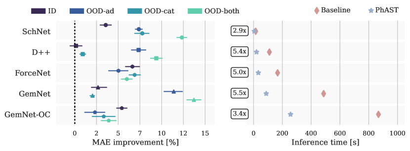
Figure 2: A comparison of the improvements brought by PhAST to the model’s MAE (left) and inference times (right) on OC20 IS2RE. MAE improvements (left) are computed as in Equation 3 and values to the right of the dashed line at 0.0 denote an improvement of PhAST with respect to the baseline. The results are averaged over 3 runs, with bootstrapped confidence intervals represented by small horizontal bars. PhAST leads to a significant MAE improvement for each validation split, up to $13\leavevmode\nobreak\ \%$, in addition to decreasing inference time (s) by several factors (e.g. 3.4$\times$ or 5.4$\times$). Absolute numerical values are provided in Section 4.2.

Baseline / MAE	ID	OOD-ad	OOD-cat	OOD-both	Average	Inference time (s)
5pt. SchNet	$637$	$734$	$661$	$703$	$683$	$15\pm 0.49$
PhAST-SchNet	$618$	$677$	$611$	$616$	630	$\boldsymbol{5\pm 0.36}$
5pt. D++	$571$	$722$	$561$	$661$	$628$	$110\pm 0.57$
PhAST-D++	$568$	$654$	$560$	$597$	595	$\boldsymbol{20\pm 0.63}$
5pt. ForceNet	$658$	$701$	$632$	$628$	$654$	$167\pm 0.96$
PhAST-ForceNet	$612$	$664$	$592$	$597$	616	$\boldsymbol{33\pm 0.60}$
5pt. GemNet	$573$	$808$	$571$	$744$	$674$	$487\pm 0.24$
PhAST-GemNet	$559$	$713$	$558$	$648$	$\boldsymbol{619}$	$\boldsymbol{88\pm 0.10}$
5pt. GemNet-OC	$593$	$658$	$605$	$584$	$610$	$868\pm 1.89$
PhAST-GemNet-OC	$564$	$636$	$587$	$562$	588	$\boldsymbol{257\pm 0.09}$

Table 1: MAE and inference time for various GNNs and their PhAST counterpart on OC20 IS2RE, averaged over 3 runs. Average MAE is computed over all validation splits. PhAST models all show improved accuracy and drastic speedups. Note that PhAST-SchNet almost matches the original DimeNet++ while being 21 times faster. A graphical visualisation of the inference time and of relative MAE improvement is provided in Figure 2. Seamingly bad MAE results for the two GemNet models are explained in Section B.2.

Results. From Section 4.2 and Figure 2, we conclude that our set of PhAST enhancements consistently improve both MAE and inference time upon the original baselines. More precisely, PhAST improves Average MAE over the four validation splits by $\sim 6.2\leavevmode\nobreak\ \%$ on average across baselines, while reducing model inference time by $\sim 4.5\times$ (on average across all baselines). Moreover, we observe an MAE improvement of 12.4 % for SchNet and 9.7 % for DimeNet++ on val OOD-both, compared to a 7.7 % and 5.2 % for Average MAE. This suggests that PhAST models generalise better than original baselines. From the ablation study conducted in LABEL:sec:ablation, we conclude that this is due to the combination of our extensions, as they all contribute to significantly better performance on out-of-distribution adsorbate-catalyst systems (OOD-both). Note that inference time gains with PhAST are almost doubled from SchNet, a 1-hop message passing (MP) approach, to DimeNet++, a 2-hops MP approach (from 3$\times$ to 5.5$\times$ speedup). Throughput scores provided in LABEL:app:tab:throughput-is2re support the results obtained from inference time.

4.3 PhAST performance on S2EF

Dataset. In this section, we focus on the Structure to Energy and Forces (S2EF-2M) OC20 dataset, that is, the prediction of both the overall energy and atom forces, from a set of 2 million 3D material structures. According to the dataset creators, the 2M split closely approximates the much more expensive full S2EF dataset, making it suitable for model evaluation (Gasteiger et al., 2022). It also come with pre-defined train/val/test splits.

Metrics. Both Energy MAE (E-MAE) and Forces MAE (F-MAE) are used to measure model accuracy. Regarding scalability, we continue to use the inference time (seconds) over the ID validation set as well as the number of samples per seconds processed by the model at inference time (throughput).

Baselines. We re-use the same baselines as above, leaving aside GemNet and GemNet-OC given the increased computational scale of this new dataset and the size of those two models. Since ForceNet already has a direct force prediction head, unlike SchNet and D++, we implemented ForceNet-FE which computes forces as the gradient of the energy with respect to atom positions (denoted FE, i.e. from energy) in order to assess the added value of the force head. PhAST-FE includes the components of the previous subsection (graph creation, atom embedding, energy head) and computes forces using the energy gradient while PhAST additionally contains the best performing force head, determined in LABEL:sec:ablation.

Results. From LABEL:tab:best-perf-s2ef, we conclude that (1) PhAST-FE improvements are also very significant on S2EF. They lead to better modeling accuracy ($13\%$ E-MAE improvement) and lower compute time (inference time divided by $4.4$) across all three models. (2) Including the proposed PhAST force-head yields significantly better energy MAE than original PhAST-FE and it reduces memory usage by a factor of 2 to 4 as well as compute time by a smaller factor.

PhAST improves Energy MAE by $32\%$ compared to base models and by $22\%$ compared to PhAST-FE while suffering from a $7\%$ drop in Force MAE (on average across all three GNNs). Compared to baselines, PhAST multiplies throughput by 10-15$\times$ and divides inference time by a factor of 4-8. Compared to energy-focused PhAST enhancements, it reduces inference time by $31\%$ on average and increases throughput by a factor of $2.4\times$. These scalability gains arise both from avoiding to compute the gradient and from increasing batch size given saved memory space. Lastly, we manage to make force prediction slightly more energy-conserving by using the gradient-target loss term, although the improvement is relatively small. A more detailed analysis can be found in LABEL:sec:ablation.

5.2 Selecting S2EF PhAST components

LABEL:tab:best-perf-s2ef contains the result of an ablation study comparing the options described in Sections 3.4 and 4.3 to adapt PhAST to the OC20 S2EF data set. We study the accuracy / scalability trade-off of the following combinations:

1. FE: original model, with forces predicted as the gradient of the energy prediction with respect to atom positions.

2. PhAST-FE: PhAST enhancement of a baseline GNN model, with components selected in the IS2RE ablation study (LABEL:subsec:ablation-is2re).

3. PhAST-Direct: PhAST model with the proposed direct force head.

4. PhAST-Grad: PhAST model with direct force head and energy-grad loss from Eq.1.

5. PhAST-Cos: PhAST model with direct force head and cosine similarity loss from Eq.2.

Additionally, we expect generative models to play a prominent role in catalyst discovery, replacing manual suggestion of promising new catalyst. In this paradigm, generative models require millions of calls to a GNN oracle to assess how good each catalyst is and explore the space of potential candidates accordingly. Due to its significant computational and accuracy gains, we believe that PhAST holds the potential to make a real difference, enabling the discovery of superior catalysts. This could lead to more efficient electrochemical reactions and thus contribute to reducing carbon emissions in industrial processes like fertilizer, cement, and green hydrogen production.

Acknowledgments and Disclosure of Funding

This research is supported in part by ANR (French National Research Agency) under the JCJC project GraphIA (ANR-20-CE23-0009-01) as well as Samsung and Intel and was made possible thanks to Fragkiskos D. Malliaros, who also provided valuable feedback all along. Alexandre Duval acknowledges support from a Mitacs Globalink Research Award. Alex Hernandez-Garcia acknowledges the support of IVADO and the Canada First Research Excellence Fund. David Rolnick acknowledges support from the Canada CIFAR AI Chairs Program. The authors also acknowledge material support from NVIDIA and Intel in the form of computational resources, and are grateful for technical support from the Mila IDT team in maintaining the Mila Compute Cluster. The authors acknowledge the support of Kin Long Kelvin Lee in performing relevant training experiments on 4th Gen Intel Xeon Scalable Processors known as Sapphire Rapids.

Appendix A Method

A.1 Invariance and equivariance to symmetries

Let $\phi:V\rightarrow{\mathbb{R}}$ and $\Phi:V\rightarrow W$ be arbitrary functions where W,V are linear spaces. Let $G$ be a group describing a symmetry which we want to incorporate into $\phi$, $\Phi$ (e.g. euclidean symmetries $E(3))$. We use group representations $\rho_{1}:G\rightarrow GL(V)$ and $\rho_{2}:G\rightarrow GL(W)$, where $GL(V)$ is the space of invertible linear maps $V\rightarrow V$ to represent how the symmetries $g\in G$ are applied to vectors $X\in V,W$. $\phi$ is an G-invariant function if it satisfies $\phi(\rho_{1}(g)X)=\phi(X)$, $\forall g\in G$ and $X\in V$. $\Phi$ is an G-equivariant function if it satisfies $\Phi(\rho_{1}(g)X)=\rho_{2}(g)\Phi(X)$, $\forall g\in G$ and $X\in V$.

In this paper, we focus on accelerated catalysis and thus on adslab relaxed adsorption energy prediction. Like for most 3D molecular prediction tasks, we want GNNs to predict the same energy for two rotated, translated or reflected versions of the same system, since their energy is equal in real-life. Hence, we target $E(3)$-invariant models, where $E(3)$ is the Euclidean group in a 3D space (we have 3D atom positions), that is, the transformations of that 3D space that preserve the Euclidean distance between any two points (i.e. rotations, reflections, translations). Note that we do desire reflection invariance because we rotate the whole adsorbate-catalyst system and not just the adsorbate, in which case chiral molecules may have a different behaviour and shall be considered distinctly.

A.2 Graph creation

A.2.1 OC20

Chanussot, Lowik, et al. Chanussot et al. (2021) create each OC20 sample by choosing a bulk material from the Materials Project database. Then, they select a surface from the bulk using Miller indices (at random) and replicate it at depth of at least $7\textup{\leavevmode\nobreak\ \AA}$ and a width of at least $8\textup{\leavevmode\nobreak\ \AA}$. The final slab is defined by a unit cell that is periodic in all directions with a vacuum layer of at least $20\textup{\leavevmode\nobreak\ \AA}$ applied in the $z$ direction. Next, they pick a binding site on this surface to attach the adsorbate onto the catalyst. The graph is now a set of atoms with their 3D positions. Last but not least, edges are created between any two nodes within a cutoff distance $c=6\textup{\AA}$ of each other (considering periodic boundary conditions).

A.2.2 PhAST graph creation process

Although well grounded, the assumptions of this graph creation process are rarely questioned. We do, with the objective of making the graph sparser and more informative for subsequent GNNs. We describe more formally the three proposals evoked in 3.1.

remove-tag-0. Let $\mathcal{S}=\{i\in\mathcal{V}:t_{i}=0\}$ denote the set of tag 0 atoms in the atomic system. The new graph we derive has attributes ${\boldsymbol{X}}={\boldsymbol{X}}_{\mathcal{S}}$ where ${\boldsymbol{X}}_{\mathcal{S}}$ is the position of all atoms except those in $\mathcal{S}$. Similarly, ${\boldsymbol{Z}}={\boldsymbol{Z}}_{\mathcal{S}}$ and ${\boldsymbol{T}}={\boldsymbol{T}}_{\mathcal{S}}$. The new adjacency matrix ${\boldsymbol{A}}_{S}$ is still defined based on cutoff distance and periodic boundary conditions: $A_{ij}=1\textrm{\ if\ }||{\boldsymbol{x}}_{i}-{\boldsymbol{x}}_{j}||<c$, $0$ otherwise. But it focuses on ${\boldsymbol{X}}_{\mathcal{S}}$, thus only containing edges which do not involve atoms in $\mathcal{S}$. Same for cell offsets $\mathbf{O}$.

one-supernode-per-graph. The position of the created super node is the mean of its components: ${\boldsymbol{x}}_{s}=\frac{1}{|\mathcal{S}|}\sum_{i\in\mathcal{S}}{\boldsymbol{x}}_{i}$ (with $\mathcal{S}$ as defined above). We associate it to a new characteristic number $z_{s}$ (corresponding to a new element in atomic table) and adjacency $A_{is}=\max(a_{ij}:j\in\mathcal{S})$. We now remove all tag-0 atoms using the remove-tag-0 method, and finally add a tag-0 attribute $t_{i}=0$ to the supernode. Note that we also remove self-loop for the supernode.

one-supernode-per-atom-type. This extension is similar to the previous one, except that we create one supernode for each chemical element in the sub-surface catalyst. This complexify a bit the graph definition. Let $a$ be the number of distinct elements with tag 0 in the graph ($a=1,2,3$ by construction) and $a_{k}$ be their characteristic number. Let $\mathcal{S}_{a_{k}}=\{i\in\mathcal{V}|t_{i}=0\textrm{\ and\ }z_{i}=a_{k}\}$ be the set of atoms corresponding to each distinct tag-0 element $a_{k}$. Each supernode $s_{k}$ is defined with $x_{s_{k}}=\frac{1}{|\mathcal{S}_{a_{k}}|}\sum_{i\in\mathcal{S}_{a_{k}}}{\boldsymbol{x}}_{i}$, $z_{k}=a_{k}$, $A_{is_{k}}=\max(A_{ij}:j\in\mathcal{S}_{a_{k}})$ ($\forall i\in\mathcal{V}$) and $A_{s_{k^{\prime}}s_{k}}=1$, $A_{s_{k}s_{k}}=0$.

For both super-node methods, we encode the number of tag-0 nodes aggregated into each super node with Positional Encodings ((Vaswani et al., 2017)) to represent their "cardinal".

A.3 Atom properties for the Embedding block

In atom embeddings, we use the following properties from the mendeleev Python package (Mentel ):

1. atomic radius,

2. atomic volume

3. atomic density

4. dipole polarizability

5. electron affinity

6. electronegativity (allen)

7. Van-Der-Walls radius

8. metallic radius

9. covalent radius

10. ionization energy (first and second order).

Appendix B Results

B.1 Hyperparameters

Hyperparameters. We use each method’s optimal set of parameters, provided in the config folder of the OCP repository for the IS2RE task, for the full dataset: https://github.com/Open-Catalyst-Project/ocp/tree/main/configs/is2re/all. Since ForceNet was not applied to IS2RE before, we adapted its S2EF configuration file to fit the IS2RE task. The only change is the smaller number of epochs used for DimeNet++ (10 instead of 20) and SchNet (20 instead of 30), as these additional epochs only lead to a small performance gain for a large amount of additional compute time.

B.2 GemNet IS2RE results

Results provided in Section 4.2 should appear surprising: both GemNet and GemNet-OC report much better results on IS2RE than we show. This is due to the fact that there are, in general, two ways to obtain the relaxed energy: either through direct prediction as we have explained in the paper, or through relaxation. The latter relies on an S2EF model that is iteratively applied to relax the system (positions are updated for the next step according to the current atom positions and associated predicted forces) until convergence, and the energy of the final (relaxed) structure is considered the model’s output energy. This procedure is both more precise (yields better Energy MAE) but also much more computationally expensive. Both GemNet and GemNet-OC report the iterative relaxation-based relaxed energy prediction method to evaluate the performance of the models on IS2RE, while training on the much larger S2EF data set.

In addition, as explained in Section 4.2 we use the published hyper parameters. We could not afford the cost of a direct-IS2RE hyper parameter search on GemNet and GemNet-OC and therefore resulted to use their S2EF hyper parameters.

All in all, while the absolute values of Energy MAE may seem surprising, the point of Figure 2 and Section 4.2 is mainly to measure the relative effects of PhAST on the individual models.

B.3 Throughput results on IS2RE

In LABEL:app:tab:throughput-is2re, we include throughput results for IS2RE models.

For a very wide range of learning rates, the training loss consistently reached NaN values.

Method / MAE	Average	ID	OOD-ad	OOD-cat	OOD-both	Inference time (s)
5pt. tag-embed	640†	639†	690†	616†	617†	168.64 +/- 0.73
phys-embed	653†	657†	702	626†	627†	172.04 +/- 0.98
l-phys-embed	667	654†	734	626†	650	167.98 +/- 0.71
pg	634†	644†	669†	618†	603†	170.70 +/- 0.96
All	637†	622†	680†	603	615†	169.23 +/- 0.84
5pt. remove-tag-0	628†	637†	668†	611†	598†	$\boldsymbol{17.06}$ +/- $\boldsymbol{0.58}$
sn-graph	635†	640†	676†	617†	607†	55.30 +/- 1.86
sn-atom-type	632†	641†	672†	616†	601†	70.55 +/- 0.15
5pt. w-init	639†	639†	687†	611†	616†	170.71 +/- 0.60
w-final	660	655†	716	627†	644	170.72 +/- 1.61
hoscpool	655	621†	703	638	638	202.03 +/- 1.23
5pt. ForceNet	654	658	701	632	628	167.08 +/- 0.52

Table 7: ForceNet ablation study on OC20 IS2RE.

B.5 Graph-Rewiring: impact on the number of edges and nodes

Rewiring	Atoms	Edges
Train
Full graph	35 789 459	1 309 308 840
remove-tag-0	32.53%	16.61%
one-supernode-per-graph	33.81%	17.76%
one-supernode-per-atom-type	35.45%	19.09%
ID
Full graph	1 939 553	70 825 106
remove-tag-0	32.54%	16.65%
one-supernode-per-graph	33.83%	17.80%
one-supernode-per-atom-type	35.47%	19.13%
OOD-ads
Full graph	1 918 704	69 877 652
remove-tag-0	32.42%	16.50%
one-supernode-per-graph	33.72%	17.64%
one-supernode-per-atom-type	35.38%	18.97%
OOD-cat
Full graph	1 917 954	70 314 085
remove-tag-0	32.88%	16.78%
one-supernode-per-graph	34.18%	17.95%
one-supernode-per-atom-type	35.90%	19.34%
OOD-both
Full graph	2 094 709	80 074 123
remove-tag-0	31.12%	15.33%
one-supernode-per-graph	32.31%	16.37%
one-supernode-per-atom-type	34.17%	17.83%

Table 8: Comparison of the number of nodes and edges in the original 5 datasets (training and 4 validation splits) and the remaining number of nodes and edges after the various rewiring strategies are performed. We can see that our rewiring methods generally remove 65+% of the atoms and 80+% of the edges.

References

- Adams et al. (2021) Keir Adams, Lagnajit Pattanaik, and Connor W Coley. Learning 3d representations of molecular chirality with invariance to bond rotations. arXiv preprint arXiv:2110.04383, 2021.
- Anderson et al. (2019) Brandon Anderson, Truong Son Hy, and Risi Kondor. Cormorant: Covariant molecular neural networks. Advances in neural information processing systems, 32, 2019.
- Batzner et al. (2022) Simon Batzner, Albert Musaelian, Lixin Sun, Mario Geiger, Jonathan P Mailoa, Mordechai Kornbluth, Nicola Molinari, Tess E Smidt, and Boris Kozinsky. E (3)-equivariant graph neural networks for data-efficient and accurate interatomic potentials. Nature communications, 13(1):1–11, 2022.
- Brandstetter et al. (2021) Johannes Brandstetter, Rob Hesselink, Elise van der Pol, Erik Bekkers, and Max Welling. Geometric and physical quantities improve e (3) equivariant message passing. arXiv preprint arXiv:2110.02905, 2021.
- Chanussot et al. (2021) Lowik Chanussot, Abhishek Das, Siddharth Goyal, Thibaut Lavril, Muhammed Shuaibi, Morgane Riviere, Kevin Tran, Javier Heras-Domingo, Caleb Ho, Weihua Hu, et al. Open catalyst 2020 (oc20) dataset and community challenges. ACS Catalysis, 11(10):6059–6072, 2021.
- Chen et al. (2019) Chi Chen, Weike Ye, Yunxing Zuo, Chen Zheng, and Shyue Ping Ong. Graph networks as a universal machine learning framework for molecules and crystals. Chemistry of Materials, 31(9):3564–3572, 2019.
- Chmiela et al. (2017) Stefan Chmiela, Alexandre Tkatchenko, Huziel E Sauceda, Igor Poltavsky, Kristof T Schütt, and Klaus-Robert Müller. Machine learning of accurate energy-conserving molecular force fields. Science advances, 3(5):e1603015, 2017.
- Duval and Malliaros (2022) Alexandre Duval and Fragkiskos Malliaros. Higher-order clustering and pooling for graph neural networks. arXiv preprint arXiv:2209.03473, 2022.
- Fuchs et al. (2020) Fabian Fuchs, Daniel Worrall, Volker Fischer, and Max Welling. Se (3)-transformers: 3d roto-translation equivariant attention networks. Advances in Neural Information Processing Systems, 33:1970–1981, 2020.
- Gasteiger et al. (2021) Johannes Gasteiger, Florian Becker, and Stephan Günnemann. Gemnet: Universal directional graph neural networks for molecules. Advances in Neural Information Processing Systems, 34:6790–6802, 2021.
- Gasteiger et al. (2022) Johannes Gasteiger, Muhammed Shuaibi, Anuroop Sriram, Stephan Günnemann, Zachary Ulissi, C Lawrence Zitnick, and Abhishek Das. Gemnet-oc: developing graph neural networks for large and diverse molecular simulation datasets. arXiv preprint arXiv:2204.02782, 2022.
- Hu et al. (2021) Weihua Hu, Muhammed Shuaibi, Abhishek Das, Siddharth Goyal, Anuroop Sriram, Jure Leskovec, Devi Parikh, and C Lawrence Zitnick. Forcenet: A graph neural network for large-scale quantum calculations. arXiv preprint arXiv:2103.01436, 2021.
- Kipf and Welling (2016) Thomas N Kipf and Max Welling. Semi-supervised classification with graph convolutional networks. arXiv preprint arXiv:1609.02907, 2016.
- Klicpera et al. (2020a) Johannes Klicpera, Shankari Giri, Johannes T Margraf, and Stephan Günnemann. Fast and uncertainty-aware directional message passing for non-equilibrium molecules. arXiv preprint arXiv:2011.14115, 2020a.
- Klicpera et al. (2020b) Johannes Klicpera, Janek Groß, and Stephan Günnemann. Directional message passing for molecular graphs. arXiv preprint arXiv:2003.03123, 2020b.
- Kolluru et al. (2022) Adeesh Kolluru, Muhammed Shuaibi, Aini Palizhati, Nima Shoghi, Abhishek Das, Brandon Wood, C Lawrence Zitnick, John R Kitchin, and Zachary W Ulissi. Open challenges in developing generalizable large scale machine learning models for catalyst discovery. Preprint arXiv:2206.02005, 2022.
- Liu et al. (2021) Yi Liu, Limei Wang, Meng Liu, Xuan Zhang, Bora Oztekin, and Shuiwang Ji. Spherical message passing for 3d graph networks. arXiv preprint arXiv:2102.05013, 2021.
- (18) Łukasz Mentel. mendeleev – a python resource for properties of chemical elements, ions and isotopes. URL https://github.com/lmmentel/mendeleev.
- Miret et al. (2022) Santiago Miret, Kin Long Kelvin Lee, Carmelo Gonzales, Marcel Nassar, and Matthew Spellings. The open matsci ml toolkit: A flexible framework for machine learning in materials science. arXiv preprint arXiv:2210.17484, 2022.
- Satorras et al. (2021) Vıctor Garcia Satorras, Emiel Hoogeboom, and Max Welling. E (n) equivariant graph neural networks. In International conference on machine learning, pages 9323–9332. PMLR, 2021.
- Schütt et al. (2017) Kristof Schütt, Pieter-Jan Kindermans, Huziel Enoc Sauceda Felix, Stefan Chmiela, Alexandre Tkatchenko, and Klaus-Robert Müller. Schnet: A continuous-filter convolutional neural network for modeling quantum interactions. Advances in neural information processing systems, 30, 2017.
- Schütt et al. (2021) Kristof Schütt, Oliver Unke, and Michael Gastegger. Equivariant message passing for the prediction of tensorial properties and molecular spectra. In International Conference on Machine Learning, pages 9377–9388. PMLR, 2021.
- Shuaibi et al. (2021) Muhammed Shuaibi, Adeesh Kolluru, Abhishek Das, Aditya Grover, Anuroop Sriram, Zachary Ulissi, and C Lawrence Zitnick. Rotation invariant graph neural networks using spin convolutions. arXiv preprint arXiv:2106.09575, 2021.
- Takigawa et al. (2016) Ichigaku Takigawa, Ken-ichi Shimizu, Koji Tsuda, and Satoru Takakusagi. Machine-learning prediction of the d-band center for metals and bimetals. RSC advances, 6(58):52587–52595, 2016.
- Thölke and De Fabritiis (2022) Philipp Thölke and Gianni De Fabritiis. Torchmd-net: Equivariant transformers for neural network based molecular potentials. arXiv preprint arXiv:2202.02541, 2022.
- Thomas et al. (2018) Nathaniel Thomas, Tess Smidt, Steven Kearnes, Lusann Yang, Li Li, Kai Kohlhoff, and Patrick Riley. Tensor field networks: Rotation-and translation-equivariant neural networks for 3d point clouds. arXiv preprint arXiv:1802.08219, 2018.
- Unke and Meuwly (2019) Oliver T Unke and Markus Meuwly. Physnet: A neural network for predicting energies, forces, dipole moments, and partial charges. Journal of chemical theory and computation, 15(6):3678–3693, 2019.
- Vaswani et al. (2017) Ashish Vaswani, Noam Shazeer, Niki Parmar, Jakob Uszkoreit, Llion Jones, Aidan N Gomez, Łukasz Kaiser, and Illia Polosukhin. Attention is all you need. Advances in neural information processing systems, 30, 2017.
- Ward et al. (2017) Logan Ward, Ruoqian Liu, Amar Krishna, Vinay I Hegde, Ankit Agrawal, Alok Choudhary, and Chris Wolverton. Including crystal structure attributes in machine learning models of formation energies via voronoi tessellations. Physical Review B, 96(2):024104, 2017.
- Xie and Grossman (2018) Tian Xie and Jeffrey C Grossman. Crystal graph convolutional neural networks for an accurate and interpretable prediction of material properties. Physical review letters, 120(14):145301, 2018.
- Ying et al. (2021) Chengxuan Ying, Tianle Cai, Shengjie Luo, Shuxin Zheng, Guolin Ke, Di He, Yanming Shen, and Tie-Yan Liu. Do transformers really perform badly for graph representation? Advances in Neural Information Processing Systems, 34:28877–28888, 2021.
- Zakeri and Syri (2015) Behnam Zakeri and Sanna Syri. Electrical energy storage systems: A comparative life cycle cost analysis. Renewable and sustainable energy reviews, 42:569–596, 2015.
- Zitnick et al. (2020) C Lawrence Zitnick, Lowik Chanussot, Abhishek Das, Siddharth Goyal, Javier Heras-Domingo, Caleb Ho, Weihua Hu, Thibaut Lavril, Aini Palizhati, Morgane Riviere, et al. An introduction to electrocatalyst design using machine learning for renewable energy storage. arXiv preprint arXiv:2010.09435, 2020.
- Zitnick et al. (2022) Larry Zitnick, Abhishek Das, Adeesh Kolluru, Janice Lan, Muhammed Shuaibi, Anuroop Sriram, Zachary Ulissi, and Brandon Wood. Spherical channels for modeling atomic interactions. Advances in Neural Information Processing Systems, 35:8054–8067, 2022.